From Local to Global Stability in Stochastic Processing Networks through Quadratic Lyapunov Functions

Abstract

We construct a generic, simple, and efficient scheduling policy for stochastic processing networks, and provide a general framework to establish its stability. Our policy is randomized and prioritized: with high probability it prioritizes jobs which have been least routed through the network. We show that the network is globally stable under this policy if there exists an appropriate quadratic ‘local’ Lyapunov function that provides a negative drift with respect to nominal loads at servers. Applying this generic framework, we obtain stability results for our policy in many important examples of stochastic processing networks: open multiclass queueing networks, parallel server networks, networks of input-queued switches, and a variety of wireless network models with interference constraints. Our main novelty is the construction of an appropriate ‘global’ Lyapunov function from quadratic ‘local’ Lyapunov functions, which we believe to be of broader interest.

1 Introduction

The past few decades have witnessed a surge in interest on the design and analysis of scheduling policies for stochastic networks, e.g., [13, 24, 18, 19, 12, 5]. One of the key insights from this body of work is that natural scheduling policies can lead to instability even when each server is nominally underloaded [15, 17, 20]. (There are several notions of stability for stochastic networks, but they intuitively entail that, in some sense, the number of customers in the system does not grow without bounds.) This insight stimulated a search for tools that can characterize the stability regions of scheduling policies, i.e., the exact conditions on the arrival and service rates under which a network is stabilized by a policy.

It is the objective of this paper to study a question of a different kind: is it possible to construct a generic, simple, and efficient scheduling policy for stochastic processing networks, which leads to a (globally) stable network if all servers are (locally) nominally underloaded in some sense? To our knowledge, we are the first to answer this question within the setting of stochastic processing networks, which constitute a large class of stochastic networks capable of modeling a variety of networked systems for communication, manufacturing, and service systems (e.g., [12]). To investigate this question, the key is to determine if and how jobs from different parts of the network should be treated differently when they share the same buffer.

Various existing scheduling policies are ‘throughput optimal’ in the sense that they achieve the largest possible stability region, but these policies suffer from significant drawbacks. They typically obtain the desired stability by framing the contention resolution between buffers as an appropriate global optimization problem. This optimization problem requires central coordination between network entities, and it is computationally hard to solve if the network is large. The resulting policies, such as the max-weight policy [18, 23] and the back-pressure policy [24, 5], are not scalable and cannot cope efficiently with large networks. As a result, these throughput optimal policies do not provide a satisfactory answer to the aforementioned question.

The computational challenges surrounding existing throughput optimal policies motivate the search for easily implementable scheduling policies with provable performance guarantees but not necessarily with the throughput optimality property. This has led to the analysis of simple greedy scheduling policies for a variety of special classes of stochastic processing networks: open multiclass queueing networks [3], input-queued switches [6], and wireless network models [16]. These policies play an important role in this paper, since our most critical assumption roughly requires any local network component to be nominally underloaded under any ‘maximal’ greedy scheduling policy.

Our main contribution is a randomized scheduling policy for stochastic processing networks which only requires coordination within local components (e.g., service stations), and which is computationally attractive since it is a kind of priority policy. With high probability, our policy prioritizes jobs which have been least routed, and we therefore call our policy the $\varepsilon$-Least Routed First Served ($\varepsilon$-LRFS) policy. Here $\varepsilon\geq 0$ is a small number which helps to make the meaning of “high probability” precise.

Our main technical tool is a novel framework to construct a ‘global’ Lyapunov function for a stochastic processing network through appropriate ‘local’ Lyapunov functions. If the local Lyapunov functions yield stability of the corresponding ‘local’ network components, then the global Lyapunov function allows us to conclude that the whole network is stable. A critical feature of our framework is that the Lyapunov functions we work with are quadratic. Through examples, we show that quadratic local Lyapunov functions can readily be found for wide classes of networks. We refer to [8, 14] for other uses of quadratic Lyapunov functions.

Our approach to construct an appropriate ‘global’ Lyapunov function using ‘local’ quadratic Lyapunov functions contrasts with the popular fluid model methodology for establishing stability of stochastic networks [3, 9, 20]. The fluid model framework essentially reduces the question of stochastic stability to a question of a related deterministic (fluid) system. In the case of reentrant lines, our policy reduces to the First Buffer First Served (FBFS) policy, which has been proven to be stable via ‘inductive’ fluid arguments [7]. A similar fluid induction argument can be expected to work for general multiclass networks (modulo some technical arguments), but a fluid induction argument cannot be expected to work in general. A disadvantage compared to fluid models is that we have to keep track of detailed system behavior such as remaining service times, but therein also lies the power of our approach. The generality of our framework presents challenges to the use of fluid methods, and instead we work directly with a global Lyapunov function. The connection with fluid techniques is discussed in more detail in Section 4.3.

Although we believe that our methodology could be of much wider use, we have chosen to work out two special classes of stochastic processing networks in order to describe the implications of our techniques in relatively simple yet powerful settings: parallel server networks (including multiclass queueing networks) and communication network models (including networks of input-queued switches and wireless networks).

Our work is related to a paper by Bramson [2], who shows that open multiclass queueing networks can be stabilized by the Earliest Due Date First Served (EDDFS) policy under the ‘local’ condition that every processing unit is nominally underloaded. However, it is not known whether the EDDFS policy achieves similar results beyond the open multiclass queueing network. In fact, it is a priori unclear how to formulate a ‘local’ condition for general stochastic processing networks; our notion of ‘local’ Lyapunov function plays this role in the present paper.

This paper is organized as follows. Section 2 introduces the class of stochastic processing networks we study in this paper. Section 3 formally introduces the $\varepsilon$-LRFS policy and presents our main results. Section 4 describes our main idea using a simple network, the Rybko-Stolyar network [20]. We specialize our result to parallel server and communication network models in Section 5. All proofs are given in Section 6.

2 A Class of Stochastic Processing Networks

A stochastic processing network (SPN) consists of a set $\mathcal{I}=\{1,\dots,I\}$ of buffers, a set $\mathcal{J}=\{1,\dots,J\}$ of activities and a set $\mathcal{K}=\{1,\dots,K\}$ of processors. Each buffer has infinite capacity and holds jobs that await service. The SPNs we study in this paper have the feature that activity $j\in\mathcal{J}$ can only process jobs from a single buffer $i_{j}\in\mathcal{I}$, and that $j$ requires simultaneous possession of a set $\mathcal{K}_{j}\subseteq\mathcal{K}$ of processors. Let $\mathcal{J}_{i}$ be the set of activities capable of processing buffer $i$, i.e.,

$$\mathcal{J}_{i}~{}=~{}\{j\in\mathcal{J}:i_{j}=i\}.$$

We say that two buffers $i$ and $\ell$ are activity-interchangeable if $\{\mathcal{K}_{j}:j\in\mathcal{J}_{i}\}=\{\mathcal{K}_{j}:j\in\mathcal{J}_{\ell}\}$. We also say that buffers $i$ and $\ell$ are processor-independent if $\bigcup_{j\in\mathcal{J}_{i}}\mathcal{K}_{j}$ and $\bigcup_{j\in\mathcal{J}_{\ell}}\mathcal{K}_{j}$ are disjoint.

Network state.

We let $Q_{i}(t)\in\mathbb{Z}_{+}$ be the queue length of buffer $i$ at time $t$, i.e., the number of jobs waiting in buffer $i$ excluding those being processed. We write $V_{i}(t)\in\mathbb{R}_{+}$ for the sum of the remaining service requirements over all jobs in buffer $i$ which are currently being processed at time $t$. We use $\sigma_{j}(t)$ to denote the activity level of activity $j$ at time $t$, where we assume that $\boldsymbol{\sigma}(t)=[\sigma_{j}(t)]\in\{0,1\}^{J}$, meaning that each activity is either fully employed or not employed at all. Thus, we say that the network is non-processor-splitting.

Routing.

After departing from a buffer $i$, a job joins buffer $\ell\in\mathcal{I}$ with probability $P_{i\ell}$ and departs from the network with probability $1-\sum_{\ell}P_{i\ell}$ (independently of everything else). We write $P$ for the $I\times I$ matrix of routing probabilities.

Resource allocation.

Each activity $j$ decreases the remaining service requirement of the job it is processing at rate $\beta_{j}>0$ if $\sigma_{j}(t)=1$. It is not allowed for an activity to be interrupted before it finishes the service requirement of the job it is working on, i.e., the network is non-preemptive. We do not allow for multiple activities to work on the same job simultaneously. Furthermore, we assume that each processor $k$ has unit capacity, i.e.,

$$\sum_{j\in\mathcal{J}:k\in\mathcal{K}_{j}}\sigma_{j}(t)~{}\leq~{}1.$$

We note that this unit capacity assumption is not restrictive since in our non-processor-splitting network of $\boldsymbol{\sigma}(t)\in\{0,1\}^{I}$, a single processor $k$ with capacity $c_{k}\in\mathbb{N}$ can be replaced by $c_{k}$ copies with unit capacity, and identical activity structure inherited from the original processor. We further define the service rate vector $s(\boldsymbol{u})=\left[s_{i}(\boldsymbol{u})\right]\in\mathbb{R}_{+}^{I}$ for a (scheduling) vector $\boldsymbol{u}=[u_{j}]\in\{0,1\}^{J}$ through

$$s_{i}(\boldsymbol{u})~{}:=~{}\sum_{j\in\mathcal{J}_{i}}u_{j}\beta_{j}.$$

External arrivals.

There are external arrivals to at least one buffer. For $0\leq s\leq t$, let $A_{i}(s,t)$ be the number of external jobs arriving at buffer $i$ during the time interval $[s,t)$. We assume that $E\left[A_{i}(0,t)^{2}\right]<\infty$ for all $t<\infty$ (i.e., bounded second moment) and

$$\limsup_{t\to\infty}E\left[A_{i}(t,t+1)~{}\Big{|}~{}\big{\{}A_{1}(0,s),\dots,A_{I}(0,s):0\leq s\leq t\big{\}}\right]<\alpha_{i},$$

for constant $\alpha_{i}\in(0,\infty)$. We note that we allow for dependencies in the random processes $A_{i}(\cdot)$ and $A_{\ell}(\cdot)$ for two buffers $i$ and $\ell$. Even though it is possible for the $\alpha_{i}$ to exceed the external arrival rates, it is convenient to interpret $\alpha_{i}$ as the external arrival rate at buffer $i$. Similarly abusing terminology, we let $\boldsymbol{\lambda}=[\lambda_{i}]$ be the effective arrival rate vector, i.e.,

$$\boldsymbol{\lambda}~{}:=~{}\left(I+P+P^{2}+\cdots\right)\boldsymbol{\alpha},$$

where $\boldsymbol{\alpha}=[\alpha_{i}]$. We also say that all routes are bounded (in length) if $\inf\left\{d\in\mathbb{N}:P^{d}=0\right\}<\infty.$

Service requirements.

Once a job in buffer $i$ is selected for processing by activity $j\in\mathcal{J}_{i}$, it requires service for a random amount of time. We assume that all service times are independent, and that they are independent of the routing and external arrival processes. We also suppose that the service time distribution only depends on the buffer from which the job is processed. Writing $\Gamma_{i}$ for a generic processing time at buffer $i$, we assume that

$$E[\Gamma_{i}]=m_{i}\qquad\mbox{and}\qquad E\left[\Gamma_{i}^{2}\right]<\infty,$$

for constants $m_{i}\in(0,\infty)$. Let $\boldsymbol{\rho}=[\rho_{i}]$ denote the nominal load, i.e., $\rho_{i}=\lambda_{i}m_{i}$. We write $W_{i}(t)$ for the (expected) immediate workload in buffer $i$, which we define to be

$$W_{i}(t)~{}=~{}m_{i}Q_{i}(t)+V_{i}(t).$$ (1)

This is the expected amount of work in the $i$-th buffer given $Q_{i}(t)$ and $V_{i}(t)$. We note that our notion of immediate workload is the conditional expectation of a more common definition, and that immediate workload is defined for each buffer (as opposed to resource). We say that the network is synchronized if for all $s,t\geq 0$, $i\in\mathcal{I}$ and $j\in\mathcal{J}$,

$$A_{i}(s,t)=A_{i}(s,\lfloor t\rfloor),\qquad\mbox{ and }\qquad\Gamma_{i}=m_{i}=\beta_{j}=1\quad\mbox{with probability $1$}.$$

That is, in a synchronized network, arrivals and service completions only occur at integer time epochs.

Maximal scheduling policies.

We say that activity $j$ is maximal in a (scheduling) vector $\boldsymbol{u}=[u_{j}]\in\{0,1\}^{J}$ if there exists a processor $k\in\mathcal{K}_{j}$ such that

$$\sum_{\ell\in\mathcal{J}:\,k\in\mathcal{K}_{\ell}}u_{\ell}~{}=~{}1,$$

i.e., either activity $j$ uses each of the processors in $\mathcal{K}_{j}$ under schedule $\boldsymbol{u}$ or it cannot be employed without violating the unit capacity constraint for some processor in $\mathcal{K}_{j}$. Given a non-negative vector $\boldsymbol{w}=[w_{i}]\in\mathbb{R}_{+}^{I}$, activity $j$ is called maximal in $\boldsymbol{u}$ with respect to $\boldsymbol{w}$ if $w_{i_{j}}=0$ or $j$ is maximal in $\boldsymbol{u}$. An activity is non-maximal if it is not maximal. If all activities are maximal in $\boldsymbol{u}$ with respect to $\boldsymbol{w}$, we simply say that $\boldsymbol{u}$ is maximal with respect to $\boldsymbol{w}$. We write $\mathcal{M}(\boldsymbol{w})$ for the set of maximal scheduling vectors with respect to $\boldsymbol{w}$, i.e.,

$$\mathcal{M}(\boldsymbol{w})~{}:=~{}\left\{\boldsymbol{u}\in\{0,1\}^{J}:\mbox{$\boldsymbol{u}$ is maximal with respect to $\boldsymbol{w}$}\right\}.$$

Finally, we say that a scheduling policy is maximal if, under the policy, $\boldsymbol{\sigma}(t)\in\mathcal{M}(\boldsymbol{Q}(t))$ for all $t\geq 0$.

3 Main Result

This section describes the scheduling policies which play a central role in this paper, and presents our main stability result.

Scheduling policies.

Our policies require that each job maintains a ‘counter’ for the number of times it has been routed so far, where we follow the convention that counters start from $1$. The counter of a job is increased even when a job is routed to a buffer it has previously visited, so the counter of a job could differ from the number of different stations it has visited. We also consider a partition $\{\mathcal{I}^{(h)}:h\in\mathcal{H}=\{1,\dots,H\}\}$ of buffers into components, such that

$$\mathcal{I}=\bigcup_{h\in\mathcal{H}}\mathcal{I}^{(h)},$$

where any two buffers from different components are processor-independent. One possible choice for the partition is $\mathcal{I}=\mathcal{I}^{(1)}$, but, as becomes apparent from the description of our policies below, a finer partition makes our policies more ‘distributed’. It is important to note that we allow for routing between components. We assume that each component $\mathcal{I}^{(h)}$ for $h\in\mathcal{H}$ maintains a ‘timer’ $\mathcal{T}^{(h)}(t)\in[0,1]$ at time $t$ which decreases at unit rate if $\mathcal{T}^{(h)}(t)>0$.

To describe our maximal scheduling policies, we need the following notation. We write $\boldsymbol{Q}^{(h)}(t)=\left[Q_{i}(t)I_{\mathcal{I}^{(h)}}(i)\right]$ for the queue length information in component $\mathcal{I}^{(h)}$, where $I_{S}\in\{0,1\}$ is the indicator function of the set $S$, i.e.,

$$I_{S}(i)~{}=~{}\begin{cases}1&\mbox{if $i\in S$}\\ 0&\mbox{otherwise}\end{cases}.$$

The following policy plays a key role throughout this paper.

Definition 3.1 (Least Routed First Served (LRFS) policy).

For each $h\in\mathcal{H}$, whenever a new arrival and/or service completion occurs at time $t$ in component $\mathcal{I}^{(h)}$, execute the following algorithm immediately after all arrivals and service completions have occurred:

• Find the set $\Sigma$ of non-maximal activities in $\boldsymbol{\sigma}(t)$ with respect to $\boldsymbol{Q}^{(h)}(t)$.

• Find a job with the smallest counter among those in buffers $\{i_{j}:j\in\Sigma\}$, where ties are broken arbitrarily.

• Choose an arbitrary activity $j\in\Sigma$ to process the job identified in step 2, i.e., set $\sigma_{j}(t)=1$.

• Repeat steps 1–3 until $\boldsymbol{\sigma}(t)$ is maximal with respect to $\boldsymbol{Q}^{(h)}(t)$.

We next introduce the maximal scheduling policy which is of primary interest in this paper. It uses a small parameter $\epsilon>0$ in order to deal with unbounded route lengths.

Definition 3.2 ($\varepsilon$-Least Routed First Served ($\varepsilon$-LRFS) policy).

For each $h\in\mathcal{H}$, whenever a new arrival and/or service completion occurs at time $t$ in component $\mathcal{I}^{(h)}$, execute the following algorithm immediately after all arrivals and service completions have occurred:

• Find a buffer $i\in\mathcal{I}^{(h)}$ containing a job with the largest counter among those in buffers $\mathcal{I}^{(h)}$.

• Find the set of non-maximal activities $\Sigma\subset\mathcal{J}_{i}$ in $\boldsymbol{\sigma}(t)$.

• If $\Sigma\neq\emptyset$ and $\mathcal{T}^{(h)}(t)=0$,

  • With probability $\varepsilon$, choose an arbitrary activity $j\in\Sigma$ to process the job identified in step 1, i.e., set $\sigma_{j}(t)=1$. With probability $1-\varepsilon$, do nothing.

  • Set $\mathcal{T}^{(h)}(t)=1$.

• Execute the LRFS policy for component $\mathcal{I}^{(h)}$.

We remark that the $\varepsilon$-LRFS policy is identical to the LRFS policy when either $\varepsilon=0$ or $\mathcal{T}^{(h)}(t)>0$, i.e., execution of the first three steps is not necessary in these cases. Since we assume that each timer decreases at unit rate, step 3-1 can be executed at most once per component in any time interval of unit length.

The network process.

Write $Q_{i,c}(t)$ for the queue length of jobs with counter $c$ in buffer $i$ at time $t$. Let $V_{i,c}^{j}(t)$ be the remaining service requirement of the job with counter $c$ in buffer $i$ at time $t$ if it is processed by activity $j$, and set $V_{i,c}^{j}(t)=0$ if $j$ is not processing a job with counter $c$. The network state is described by

$$X(t)~{}=~{}\left[Q_{i,c}(t),V_{i,c}^{j}(t),\mathcal{T}^{(h)}(t)~{}:~{}i\in\mathcal{I},j\in\mathcal{J},c\in\mathbb{N},h\in\mathcal{H}\right]~{}\in~{}\Omega_{X}:=\left(\mathbb{Z}_{+}^{I}\times\mathbb{R}_{+}^{I\times J}\right)^{\infty}\times[0,1]^{H}.$$

Note that $X(t)$ does not encode information on the external arrival processes. In particular, $\{X(t)\}$ is non-Markovian in general. We impose the convention that $\{X(t)\}$ has right-continuous sample paths. We define a norm on $\Omega_{X}$ through

$$|X(t)|~{}=~{}\sum_{i\in\mathcal{I},c\in\mathbb{N}}Q_{i,c}(t)+\sum_{i\in\mathcal{I},c\in\mathbb{N},j\in\mathcal{J}}V_{i,c}^{j}(t).$$

We assume that $X(0)\in\Omega_{X}^{*}$ where $\Omega_{X}^{*}=\{X\in\Omega_{X}:|X|<\infty\}$. In synchronized networks, one has $V^{j}_{i,c}(t)\in\{0,1\}$ for all $t\in\mathbb{Z}_{+}$ under the $\varepsilon$-LRFS policy. We refer to the process $\{X(t):t\in\mathbb{R}_{+}\}$ operating under the $\varepsilon$-LRFS policy as the $\varepsilon$-LRFS process. If $\varepsilon=0$, then we simply refer to this process as the LRFS process.

Network stability.

This paper uses the following notion of stability.

Definition 3.3.

The $\varepsilon$-LRFS process $\{X(t)\}$ is called queue-length-stable if

$$\limsup_{t\to\infty}\frac{1}{t}\int_{0}^{t}E\left[|X(s)|\right]ds<\infty,$$ (2)

for any given initial state $X(0)\in\Omega_{X}^{*}$.

We establish the queue-length-stability by constructing appropriate Lyapunov functions. Under some additional assumptions on the arrival processes and service time distributions, these Lyapunov functions can also be used to establish positive recurrence of the $\varepsilon$-LRFS process, cf. Condition (A3) in [4]. It is outside of the main scope of the current paper to work out the details. We also remark that our proof can find an explicit finite constant for the right-hand side of (2), but this requires tedious bookkeeping and we therefore do not carry out this analysis.

To show the desired stability, we need the following notion of a ‘local’ Lyapunov function.

Definition 3.4.

We say that $\mathcal{L}_{\mathrm{local}}:\mathbb{R}_{+}^{I}\to\mathbb{R}_{+}$ is a local Lyapunov function with slack parameter $\varepsilon\geq 0$ if there exist constants $\mathcal{C}\geq 0$, $\eta>0$ such that for every pair $(\boldsymbol{w},\boldsymbol{u})\in\mathbb{R}_{+}^{I}\times\{0,1\}^{J}$ satisfying $\boldsymbol{u}\in\mathcal{M}(\boldsymbol{w})$,

$$\mathcal{L}_{\text{\em local}}\Big{(}\boldsymbol{w}+\boldsymbol{\rho}+\varepsilon\boldsymbol{m}-s(\boldsymbol{u})\Big{)}~{}\leq~{}\mathcal{L}_{\text{\em local}}(\boldsymbol{w})-\eta\|\boldsymbol{w}\|_{1}+\mathcal{C},$$ (3)

where $\boldsymbol{m}=[m_{i}]\in\mathbb{R}^{I}$.

The reason for this nomenclature is that in a ‘local’ network, i.e., a network without routing ($P=0$), the above inequality for $\mathcal{L}_{\mathrm{local}}$ provides the desired negative drift condition in the Foster-Lyapunov criteria [10], which implies network stability. Here $w_{i}$, $\rho_{i}$, and $s_{i}(\boldsymbol{u})$ can be interpreted as the immediate workload, the external workload arrival rate and the workload processing rate at buffer $i$, respectively. We refer to Sections 4 and 5 for examples of local Lyapunov functions.

Now we are ready to state the main theorem of this paper, which establishes ‘global’ stability using a ‘local’ quadratic Lyapunov function.

Theorem 3.5.

Suppose that there exists a symmetric matrix $Z\in\mathbb{R}_{+}^{I\times I}$ such that $\mathcal{L}_{\mathrm{local}}(x)=x^{T}Zx$ is a local Lyapunov function with slack $\varepsilon>0$. Then the $\varepsilon$-LRFS process is queue-length-stable if one of the following conditions C1 and C2 is satisfied:

• The network is synchronized and $Z_{i\ell}\neq 0$ only if buffers $i$ and $\ell$ are in the same component.

• $Z_{i\ell}\neq 0$ only if buffers $i$ and $\ell$ are activity-interchangeable and every buffer $i$ has an associated activity $j\in\mathcal{J}_{i}$ with $|\mathcal{K}_{j}|=1$.

Furthermore, if all routes are bounded, then the LRFS process is queue-length-stable if one of the conditions C1 or C2$\,{}^{\prime}$ is satisfied, where

• $Z_{i\ell}\neq 0$ only if buffers $i$ and $\ell$ are activity-interchangeable.

Theorem 3.5 implies that if any maximal policy is ‘quadratic’ stable in a stochastic processing network without routing under the external load $\boldsymbol{\rho}$, then $\varepsilon$-LRFS is stable in a stochastic processing network with routing under nominal load $<\boldsymbol{\rho}$ for some small $\varepsilon>0$. Section 4 describes the main idea of the proof, and a full proof is presented in Section 6.

We remark that the requirement of activity-interchangeable buffers in Condition C2 can be relaxed slightly. Our proof of Theorem 3.5 also works when the following relaxed condition C3 replaces C2.

• $Z_{i\ell}\neq 0$ only if for every $j\in\mathcal{J}_{i}$, there exists $j^{\prime}\in\mathcal{J}_{\ell}$ such that $\mathcal{K}_{j^{\prime}}\subseteq\mathcal{K}_{j}$, and vice versa (i.e., for every $j\in\mathcal{J}_{\ell}$, there exists $j^{\prime}\in\mathcal{J}_{i}$ such that $\mathcal{K}_{j^{\prime}}\subseteq\mathcal{K}_{j}$). Also, every buffer $i$ has an associated activity $j\in\mathcal{J}_{i}$ with $|\mathcal{K}_{j}|=1$.

A corresponding condition C3$\,{}^{\prime}$ can also replace C2$\,{}^{\prime}$, where C3$\,{}^{\prime}$ does not require the second part of C3.

4 Proof Ideas for Theorem 3.5

In this section, we describe the main idea in the proof of Theorem 3.5. We first present it in a very special network, the Rybko-Stolyar network [20], which allows us to summarize the main idea of the proof at a high level. We subsequently describe the challenges that have to be overcome to establish our result in the general case, and discuss the feasibility of an approach based on fluid models.

4.1 Rybko-Stolyar Network

This network consists of four activities associated to four different buffers and two processors. The first processor is required for activities 1 and 4, and the second for activities 2 and 3. Each activity decreases the remaining service requirement of the job it is currently processing at unit rate (i.e., $\beta_{j}=1$). Customers (or jobs) arrive at the first and third buffers, and traverse the buffers deterministically in the order $1\to 2$ or $3\to 4$. The service time is deterministic and equal to $m_{i}$ for buffer $i$, and the external arrival processes (at the first and third buffers) are independent Poisson processes with rate 1. The network is given in Figure 1, and a necessary condition for stability is

$$\rho_{1}=m_{1}+m_{4}<1\qquad\mbox{and}\qquad\rho_{2}=m_{2}+m_{3}<1.$$ (4)

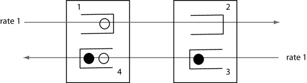
Figure 1: Illustration of the Rybko-Stolyar Network. In this diagram, there are four jobs in the system. Jobs are currently being processed and waiting for service are colored black and white, respectively.

The network state can be described by $X(t)=\{Q_{i}(t),V_{i}(t):i=1,2,3,4\}\in\Omega_{X}:=\mathbb{Z}_{+}^{4}\times\mathbb{R}_{+}^{4}$, where $Q_{i}(t)$ is the queue length (i.e., the number of jobs waiting) of buffer $i$ at time $t$ and $V_{i}(t)$ is the remaining service time of the job currently being processed in buffer $i$ at time $t$. Hence $V_{i}(t)=0$ if no job is being processed in buffer $i$. We define a norm through $|X(t)|=\sum_{i}(V_{i}(t)+Q_{i}(t))$. In this network, it is known [20] that if processor 1 prioritizes buffer 4 and processor 2 prioritizes buffer 2, the network can be unstable even when the necessary condition (4) holds. On the other hand, LRFS prioritizes buffer 1 and 3, so it reduces to the First Buffer First Served policy. This is known to be stable under the necessary stability condition (4). We next derive this stability result using our main idea.

Assuming LRFS and (4), we construct an appropriate Lyapunov function $\mathcal{L}_{\mathrm{global}}:\Omega_{X}\to\mathbb{R}_{+}$ satisfying

$$E\left[\mathcal{L}_{\mathrm{global}}(X(t+1))-\mathcal{L}_{\mathrm{global}}(X(t))~{}\Bigg{|}~{}X(t)\right] \leq -\gamma|X(t)|+\mathcal{C},\qquad\mbox{almost surely},$$ (5)

where $\gamma,\mathcal{C}>0$ are some constants. By first taking expectations with respect to the distribution of $X(t)$ and then integrating over $t$ on both sides of the above inequality, we conclude that

$$\limsup_{t\to\infty}\frac{1}{t}\int_{0}^{t}E\left[|X(s)|\right]ds \leq \limsup_{t\to\infty}\frac{1}{\gamma}\left(\mathcal{C}-\frac{\int_{t}^{t+1}E[\mathcal{L}_{\mathrm{global}}(X(s))]ds-\int_{0}^{1}E[\mathcal{L}_{\mathrm{global}}(X(s))]ds}{t}\right)$$ (6)

$$\leq \limsup_{t\to\infty}\frac{1}{\gamma}\left(\mathcal{C}+\frac{\int_{0}^{1}E\left[\mathcal{L}_{\mathrm{global}}(X(s))\right]ds}{t}\right)$$

$$= \frac{\mathcal{C}}{\gamma}~{}<~{}\infty.$$

We now proceed toward constructing the ‘global’ Lyapunov function $\mathcal{L}_{\mathrm{global}}$ satisfying (5) based on a ‘local’ quadratic Lyapunov function $\mathcal{L}_{\mathrm{local}}$. To this end, we first discuss how to construct the ‘local’ quadratic Lyapunov function. Consider a single-processor system with two buffers $a$ and $b$, deterministic service times given by $m_{a}$ and $m_{b}$, and independent Poisson arrival processes with rate $1$ at each buffer (i.e., the total rate is $2$). Hence, a necessary condition for stability is

$$m_{a}+m_{b}<1.$$

Under a maximal (i.e., work-conserving) scheduling policy, the workload $W(t)=\sum_{i}W_{i}(t)$ at time $t$ satisfies

$$W(t+1)~{}=~{}W(t)+\sum_{i=a,b}m_{i}\,A_{i}(t,t+1)-\int^{t+1}_{t}{\bf 1}^{+}_{W(u)}du,$$

where $W_{i}(t)$ is defined as the immediate workload at buffer $i$ as in (1), $A_{i}(s,t)$ is the number of jobs arriving at buffer $i$ during the time interval $[s,t)$ so that $E[A_{i}(s,t)]=t-s$ and we define

$${\bf 1}^{+}_{x}=\begin{cases}1&\mbox{if}~{}x>0\\ 0&\mbox{otherwise}\end{cases}.$$

Hence, we have

$$E\left[W(t+1)-W(t)~{}\Big{|}~{}W(t)\right]~{}\leq~{}m_{a}+m_{b}-{\bf 1}^{+}_{W(t)-1},$$ (7)

where we use that ${\bf 1}^{+}_{W(u)}\geq{\bf 1}^{+}_{W(t)-1}$ for $u\in[t,t+1]$ since we assume deterministic service times. Using this, it follows that for some finite constant $\mathcal{C}$,

$$E\left[W(t+1)^{2}-W(t)^{2}~{}\Bigg{|}~{}W(t)\right] = E\left[2W(t)(W(t+1)-W(t))~{}\Bigg{|}~{}W(t)\right]$$ (8)

$$\qquad+E\left[(W(t+1)-W(t))^{2}~{}\Bigg{|}~{}W(t)\right]$$

$$\leq 2W(t)E\left[W(t+1)-W(t)~{}\Bigg{|}~{}W(t)\right]+\mathcal{C}$$

$$\leq 2W(t)\left(m_{a}+m_{b}-{\bf 1}^{+}_{W(t)-1}\right)+\mathcal{C}$$

$$< -2(1-m_{a}-m_{b})W(t)+\mathcal{C}+2,$$

where we use $E\left[A_{i}(t,t+1)^{2}\right]<\infty$ for the first inequality. This shows that $W(t)^{2}=(W_{1}(t)+W_{2}(t))^{2}$ is a suitable Lyapunov function for our ‘local’ single-processor system under the necessary stability condition $m_{a}+m_{b}<1$.

This observation on the single-processor system motivates the following quadratic local Lyapunov function $\mathcal{L}_{\mathrm{local}}:\mathbb{R}_{+}^{I}\to\mathbb{R}_{+}$ for the Rybko-Stolyar network:

$$\mathcal{L}_{\mathrm{local}}(x)~{}=~{}x^{T}Zx~{}=~{}x^{T}\begin{pmatrix}1&0&0&1\\ 0&1&1&0\\ 0&1&1&0\\ 1&0&0&1\end{pmatrix}x~{}=~{}(x_{1}+x_{4})^{2}+(x_{2}+x_{3})^{2},\qquad\mbox{for}~{}~{}x=(x_{1},x_{2},x_{3},x_{4}).$$ (9)

One can easily check that it satisfies (3) with (small) slack $\varepsilon>0$ under the necessary stability requirements $m_{1}+m_{4}<1$ and $m_{2}+m_{3}<1$. We propose the following global Lyapunov function $\mathcal{L}_{\mathrm{global}}$:

$$\mathcal{L}_{\mathrm{global}}(X(t))~{}=~{}\mathcal{L}_{\mathrm{local}}\big{(}W_{1}(t),V_{2}(t),W_{3}(t),V_{4}(t)\big{)}+\xi\mathcal{L}_{\mathrm{local}}\left(W_{1}(t),\widehat{W}_{2}(t),W_{3}(t),\widehat{W}_{4}(t)\right),$$

where the new parameters $\xi$ and $\widehat{W}_{i}(t)$ shall be defined explicitly. We remind the reader that our goal is to prove (5).

First, a similar calculation as for the single-processor case in (7) yields that under the LRFS policy,

$$E\left[W_{1}(t+1)+V_{4}(t+1)-W_{1}(t)-V_{4}(t)~{}\Big{|}~{}X(t)\right] \leq -{\bf 1}^{+}_{W_{1}(t)+V_{4}(t)-1}+m_{1},$$

$$E\left[W_{3}(t+1)+V_{2}(t+1)-W_{3}(t)-V_{2}(t)~{}\Big{|}~{}X(t)\right] \leq -{\bf 1}^{+}_{W_{3}(t)+V_{2}(t)-1}+m_{3}.$$

Hence, as for (8), one can conclude that for some constant $\mathcal{C}$,

$$E\left[\left(W_{1}(t+1)+V_{4}(t+1)\right)^{2}-\left(W_{1}(t)+V_{4}(t)\right)^{2}~{}\Big{|}~{}X(t)\right] \leq -2(1-m_{1})(W_{1}(t)+V_{4}(t))+\mathcal{C},$$

(10)

$$E\left[\left(W_{3}(t+1)+V_{2}(t+1)\right)^{2}-\left(W_{3}(t)+V_{2}(t)\right)^{2}~{}\Big{|}~{}X(t)\right] \leq -2(1-m_{3})(W_{3}(t)+V_{2}(t))+\mathcal{C},$$

(11)

where the precise value of $\mathcal{C}$ can be different from line to line.

We note that the sum $\left(W_{1}(t)+V_{4}(t)\right)^{2}+\left(W_{3}(t)+V_{2}(t)\right)^{2}$ is not a suitable choice for $\mathcal{L}_{\mathrm{global}}$ since it does not include $Q_{2}(t)$ and $Q_{4}(t)$ (or $W_{2}(t)$ and $W_{4}(t)$). To address this issue, we further use

$$\widehat{W}_{2}(t):=W_{2}(t)+m_{2}Q_{1}(t)\qquad\mbox{and}\qquad\widehat{W}_{4}(t):=W_{4}(t)+m_{4}Q_{3}(t).$$

We refer to $\widehat{W}_{2}$ and $\widehat{W}_{4}$ as the total workload in buffer $2$ and $4$, respectively. Using this notation, one finds that under the LRFS policy,

$$E\left[W_{1}(t+1)+\widehat{W}_{4}(t+1)-W_{1}(t)-\widehat{W}_{4}(t)~{}\Big{|}~{}X(t)\right] \leq -{\bf 1}^{+}_{W_{1}(t)+W_{4}(t)-1}+m_{1}+m_{4},$$

$$E\left[W_{3}(t+1)+\widehat{W}_{2}(t+1)-W_{3}(t)-\widehat{W}_{2}(t)~{}\Big{|}~{}X(t)\right] \leq -{\bf 1}^{+}_{W_{2}(t)+W_{3}(t)-1}+m_{2}+m_{3}.$$

The above equalities can be used to obtain ‘negative drift terms’ for $W_{2}(t)$ and $W_{4}(t)$, which are missing in (10) and (11). Namely, for some constant $\mathcal{C}$, we obtain

$$E\left[\left(W_{1}(t+1)+\widehat{W}_{4}(t+1)\right)^{2}-\left(W_{1}(t)+\widehat{W}_{4}(t)\right)^{2}~{}\Big{|}~{}X(t)\right]$$

$$\qquad\qquad\leq~{}2\left(W_{1}(t)+\widehat{W}_{4}(t)\right)E\left[W_{1}(t+1)+\widehat{W}_{4}(t+1)-W_{1}(t)-\widehat{W}_{4}(t)~{}\Big{|}~{}X(t)\right]+\mathcal{C}$$

$$\qquad\qquad\leq~{}2\left(W_{1}(t)+\widehat{W}_{4}(t)\right)\left(-{\bf 1}^{+}_{W_{1}(t)+W_{4}(t)-1}+m_{1}+m_{4}\right)+\mathcal{C}$$

$$\qquad\qquad\leq~{}-2(1-m_{1}-m_{4})\left(W_{1}(t)+W_{4}(t)\right)+2(m_{1}+m_{4})m_{4}Q_{3}(t)+\mathcal{C}+2$$

$$\qquad\qquad\leq~{}-2(1-\rho_{\max})\left(W_{1}(t)+W_{4}(t)\right)+2m^{*}\rho_{\max}W_{3}(t)+\mathcal{C}+2,$$ (12)

where $\rho_{\max}=\max\{\rho_{1},\rho_{2}\}$ and $m^{*}=\max_{i,j}\left\{\frac{m_{i}}{m_{j}}\right\}$. Similarly,

$$E\left[\left(W_{3}(t+1)+\widehat{W}_{2}(t+1)\right)^{2}-\left(W_{3}(t)+\widehat{W}_{2}(t)\right)^{2}~{}\Big{|}~{}X(t)\right]$$

$$\qquad\qquad\qquad\qquad\qquad\leq-2(1-\rho_{\max})\left(W_{3}(t)+W_{2}(t)\right)+2m^{*}\rho_{\max}W_{1}(t)+\mathcal{C}+2.$$ (13)

Observe that there are positive terms $W_{3}(t)$ and $W_{1}(t)$ in (12) and (13), respectively. The key idea behind our proof is that the positive terms can be canceled out by appropriately summing (10), (11), (12) and (13). Indeed, we define the desired Lyapunov function $\mathcal{L}_{\mathrm{global}}$ as

$$\mathcal{L}_{\mathrm{global}}(X)~{}=~{}\left(W_{1}+V_{4}\right)^{2}+\left(W_{3}+V_{2}\right)^{2}+\xi\left(W_{1}+\widehat{W}_{4}\right)^{2}+\xi\left(W_{3}+\widehat{W}_{2}\right)^{2},$$

where we choose $\xi=\frac{1-\rho_{\max}}{2m^{*}\rho_{\max}}$. Combining (10), (11), (12) and (13), we conclude that

$$E\left[\mathcal{L}_{\mathrm{global}}(X(t+1))-\mathcal{L}_{\mathrm{global}}(X(t))~{}\Bigg{|}~{}X(t)\right]~{}\leq~{}-2\xi(1-\rho_{\max})|X(t)|+\mathcal{C}.$$

This completes the proof of (5), and hence the desired stability (6).

4.2 Beyond the Rybko-Stolyar Network

The preceding subsection presents the main idea behind our construction of a ‘global’ Lyapunov function $\mathcal{L}_{\mathrm{global}}$ using a ‘local’ Lyapunov function $\mathcal{L}_{\mathrm{local}}$ (i.e., from the single-processor system) in the specific example of the Rybko-Stolyar network. The construction of $\mathcal{L}_{\mathrm{global}}$ relies on summing $\mathcal{L}_{\mathrm{local}}$ terms inductively by exploring certain maximality properties of the LRFS policy at each iteration. In general networks there are several difficulties which do not arise in the Rybko-Stolyar network, and this section discusses the ideas and arguments needed to overcome them.

A first challenge we have overcome arises in networks with unbounded route lengths (i.e., $\inf\{d\in\mathbb{N}:P^{d}=0\}=\infty$). In that case, the above inductive procedure does not terminate. For this reason, we propose a variant of the LRFS policy, the $\varepsilon$-LRFS policy, which occasionally processes a job with the largest counter. Intuitively speaking, this additional mechanism in $\varepsilon$-LRFS can control the jobs with large counters, whereas LRFS cannot.

A second challenge we have surmounted is that the construction of $\mathcal{L}_{\mathrm{global}}$ in the Rybko-Stolyar network starts from a simple local Lyapunov function in a single-server system, but it is not clear whether similar arguments go through for general local Lyapunov functions and stochastic processing networks. We require Condition C2 to resolve this issue. It is readily seen that the local Lyapunov function (9) used in the Rybko-Stolyar network satisfies this condition. The condition can be relaxed under some additional conditions on the arrival processes and service time distributions. For example, in synchronized networks, Condition C1 can be used instead of C2.

A further challenge in the general case relates to the definition of $\widehat{W}_{i}(t)$. In the Rybko-Stolyar network, it is the sum of workloads along a path of buffers, with $i$ as the last buffer. This definition only applies to networks with deterministic routing. In the general case we use several notions of total workload. To allow for stochastic routing, we construct a new process $\{Y(t)\}$ from $\{X(t)\}$ with deterministic routing. This process is essentially identical to $\{X(t)\}$, but we enlarge the state space to incorporate routing information. We construct a Lyapunov function $\mathcal{L}_{\mathrm{global}}$ for $\{Y(t)\}$, which we use to establish the stability of $\{Y(t)\}$ and hence the stability of $\{X(t)\}$.

In summary, we construct the Lyapunov function $\mathcal{L}_{\mathrm{global}}$ for general networks as the sum of three parts:

$$\mathcal{L}_{\mathrm{global}}(Y(t))~{}=~{}\sum_{c=1}^{D}\left(\frac{\upsilon}{2\mathcal{C}}\right)^{c}\mathcal{L}_{\mathrm{local}}\left(\widehat{\boldsymbol{W}}_{\leq c}(t)\right)+\frac{2\mathcal{C}}{\beta_{\min}}\,\|\boldsymbol{V}(t)\|_{2}^{2}+\frac{\xi}{2\mathcal{C}}\,\mathcal{G}(Y(t))^{2}.$$

The specific notation used here is not important; we refer readers to Section 6 for the definitions used. To prove stability, we need to argue that this function satisfies a so-called negative-drift condition. The first term, i.e., the finite sum, comes from the inductive construction under LRFS, appropriately truncated. For the Rybko-Stolyar network, this is the only part we need. The first part produces the desired negative drift for jobs with low counters, but it gives a positive drift in terms of remaining service requirements $\boldsymbol{V}(t)$ as a by-product (albeit not in the Rybko-Stolyar network under the assumptions of the preceding subsection). The second term in our Lyapunov function ($\|\boldsymbol{V}(t)\|^{2}_{2}$) has a negative drift and compensates the positive drift incurred by the first term. The third term in our Lyapunov function ($\mathcal{G}(Y(t))^{2}$) controls the high-counter jobs under the mechnism which is present in the $\varepsilon$-LRFS policy but not in the LRFS policy (step 3 in Definition 3.2). This additional mechanism allows us to establish a negative drift for the last term. By appropriately weighing each of the three terms, we derive the desired negative drift condition for the Lyapunov function $\mathcal{L}_{\mathrm{global}}$.

4.3 Connection with Fluid Models

As mentioned in the previous subsection, our approach relies on an inductive argument based on job counters. For the Rybko-Stolyar network and more generally for multiclass networks, fluid models can be used to give relatively simple proofs of our results. Thus, a more detailed discussion on the connection with fluid models together with its pros and cons is warranted.

The fluid approach consists of two main steps. In the first step, by scaling time and space, one proves convergence of the queueing process to the solution of a system of deterministic equations known as the fluid model. In the second step, one proves that this fluid model is stable, i.e., that it eventually reaches the origin. Stability of the fluid model can be established through the construction of a Lyapunov function for the fluid model, or in some cases one can obtain fluid stability through direct methods such as induction. Once fluid stability has been established, one can apply general theorems to deduce that the stochastic model is also stable (in a certain sense), see for instance [3].

It might be possible to establish existence of a fluid model and to prove that the stochastic model converges to the fluid model in the setting of the present paper, and it can be expected that our ‘global’ Lyapunov function should work to prove fluid stability. Comparing our approach with this proof strategy, a disadvantage of the fluid model is that one needs to establish convergence to the fluid model, while a disadvantage of our approach is that we have to keep track of detailed state information such as residual service times.

Another possible approach to establish fluid stability is to use an inductive argument, which may seem particularly attractive given our construction of job counters and the suitability of a induction argument in existing work on fluid models [7]. However, this approach has inherent challenges. The base step in an inductive approach could use the ‘local’ Lyapunov function $\mathcal{L}_{\mathrm{local}}$ to argue that the fluid level of jobs with counter 1 vanishes after some finite time $T_{1}$. It would then use $\mathcal{L}_{\mathrm{local}}$ to argue that the fluid level of jobs with counter 2 vanishes after some finite time $T_{2}>T_{1}$, and so forth. To carry out this argument, one has to show that $\mathcal{L}_{\mathrm{local}}$ satisfies a certain negative-drift condition under the assumption that high-priority counter 1 jobs vanish on a fluid scale. The latter only yields a guarantee on the ‘average’ or ‘long-run’ behavior of the jobs with counter 1, whereas one needs ‘short-term’ network state information to establish the negative-drift condition for jobs with counter 2. Indeed, under our scheduling policy, jobs with counter 1 (even when vanishing on a fluid scale) can significantly influence the dynamics of jobs with counter 2 depending on the complexity of the network. Therefore, the base of the induction approach is too weak to be used in the induction step for general networks since one needs more detailed information than the time-average given by the fluid approach.

In special cases such as multiclass networks, one may not need quadratic Lyapunov functions and it may be possible to establish the stability of our counter-based policy using fluid induction without quadratic Lyapunov functions. However, in general (e.g., for networks of switches), we need quadratic Lyapunov functions since they are the only available tool to establish stability for single-hop networks.

5 Examples

In this section, we provide applications of Theorem 3.5 to various special stochastic processing networks. We consider parallel server networks (including multiclass queueing networks) in Section 5.1 and communication networks (including wireless networks and networks of input-queued switches) in Section 5.2. They are examples of non-synchronized and synchronized networks, respectively. In all of these important examples, suitable local Lyapunov functions are easy to find.

5.1 Open Multiclass Queueing Networks and Parallel Server Networks

In this section, we consider special stochastic processing networks known as parallel server networks. These networks are characterized by the following assumption.

• Each activity is processed by exactly one processor and processes exactly one buffer, i.e.,

  $$|\mathcal{K}_{j}|=1,\qquad\mbox{ for all}~{}~{}j\in\mathcal{J}.$$

Figure 2 illustrates the relations between buffers, activities and processors in parallel server networks. Our notion of ‘parallel server network’ generalizes the well-studied parallel server systems [11] by adding stochastic routing dynamics between buffers. It also includes open multiclass queueing networks [3] as a special case, which additionally require

$$|\mathcal{J}_{i}|=1,\qquad\mbox{ for all}~{}~{}i\in\mathcal{I}.$$ (14)

In open multiclass queueing networks, buffers and activities are in one-to-one correspondence and they are referred to as classes. The Rybko-Stolyar in Section 4 is an instance of open multiclass queueing networks.

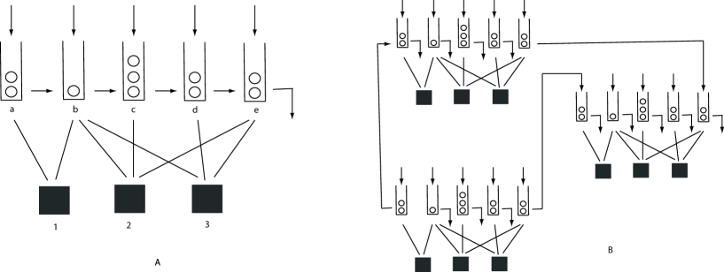
Figure 2: Two examples of parallel server networks. They do not satisfy Assumption A2. The leftmost diagram illustrates a parallel server network with five buffers $\{a,b,c,d,e\}$, three processors $\{1,2,3\}$ and eight activities $\{(a,1),(b,1),(b,2),(b,3),(c,2),(d,3),(e,2),(e,3)\}$. Once a job in buffer $a,b,c,d$ completes its service requirement, it joins buffer $b,c,d,e$ (i.e., $P_{ab}=P_{bc}=P_{cd}=P_{de}=1$), respectively. Once a job in buffer $e$ completes its service requirement, it leaves the network. The rightmost diagram illustrates a parallel server network consisting of three ‘local’ parallel server systems where jobs are routed between local systems.

A parallel server network naturally defines a bipartite graph $(\mathcal{I},\mathcal{K},\mathcal{J})$ such that each activity in $\mathcal{J}$ defines an edge between buffers $\mathcal{I}$ and processors $\mathcal{K}$. Requirement (14) of open multiclass queueing networks imposes the additional restriction that each vertex in $\mathcal{I}$ has degree one. We further consider the following strengthening of Assumption A1.

• $(\mathcal{I},\mathcal{K},\mathcal{J})$ is a union of disjoint complete bipartite graphs $\{(\mathcal{I}^{(h)},\mathcal{K}^{(h)},\mathcal{J}^{(h)}):h\in\mathcal{H}\}$, i.e.,

  $$\cup_{h\in\mathcal{H}}\mathcal{I}^{(h)}=\mathcal{I},\qquad\cup_{h\in\mathcal{H}}\mathcal{K}^{(h)}=\mathcal{K},\qquad\mbox{and}\qquad\cup_{h\in\mathcal{H}}\mathcal{J}^{(h)}=\mathcal{J}.$$

This assumption implies that two buffers in the same component are activity-interchangeable, even though they may differ with respect to routing, external arrivals or service requirements. One can easily check that open multiclass queueing networks always satisfy this assumption, while the parallel server networks in Figure 2 do not. Assumption A2 is useful because it enables us to establish a necessary condition for stability and it allows us to find a suitable local Lyapunov function satisfying Condition C2 of Theorem 3.5. However, Theorem 3.5 is applicable to general networks as long as one can find a ‘good’ local Lyapunov function satisfying Condition C2. Figure 3 gives examples of parallel server networks satisfying Assumption A2.

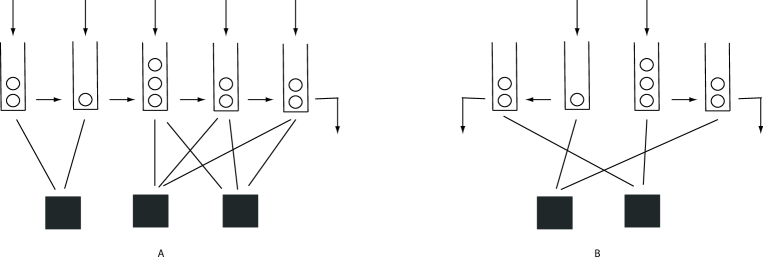
Figure 3: Two examples of parallel server networks satisfying Assumption A2. The rightmost diagram illustrates the Rybko-Stolyar network described in Section 4.

Necessary condition for stability.

We now aim to obtain a necessary condition for stability of a parallel server network. Under Assumption A2, a necessary condition to stabilize the network is that for every $n$,

$$\rho^{(h)}:=\sum_{i\in\mathcal{I}^{(h)}}\rho_{i}~{}<~{}\beta^{(h)}:=\sum_{j\in\mathcal{J}^{(h)}}\beta_{j}.$$ (15)

It is clear that the above condition is required for stability since $\rho^{(h)}$ and $\beta^{(h)}$ describe the total nominal load and the maximum processing rate, respectively, at the local component $(\mathcal{I}^{(h)},\mathcal{K}^{(h)},\mathcal{J}^{(h)})$.

Local Lyapunov function.

As in Section 4, the single-processor example is the main building block. We define the local Lyapunov function as

$$\mathcal{L}_{\mathrm{local}}(x)=\sum_{h\in\mathcal{H}}\left(\sum_{i\in\mathcal{I}^{(h)}}x_{i}\right)^{2}\qquad\mbox{for}~{}~{}x=(x_{1},\dots,x_{I}).$$ (16)

We now show that this function satisfies (3) with some slack $\varepsilon\geq 0$ as long as the necessary condition (15) for stability is satisfied. For given vectors $\boldsymbol{w}=[w_{i}]\in\mathbb{R}_{+}^{I}$ and $\boldsymbol{u}=[u_{j}]\in\mathcal{M}(\boldsymbol{w})$, maximality implies that, on writing $w^{(h)}=\sum_{i\in\mathcal{I}^{(h)}}w_{i}$,

$$s^{(h)}=s^{(h)}(\boldsymbol{u})~{}:=~{}\sum_{j\in\mathcal{J}^{(h)}}u_{j}\beta_{j}~{}\geq~{}\sum_{j\in\mathcal{J}^{(h)}}{\bf 1}^{+}_{w^{(h)}}\beta_{j}~{}=~{}{\bf 1}^{+}_{w^{(h)}}\beta^{(h)},$$

where we use Assumption A2 and we recall that ${\bf 1}^{+}_{x}=1$ if $x>0$, and ${\bf 1}^{+}_{x}=0$ otherwise. Thus, we have

$$\mathcal{L}_{\mathrm{local}}(\boldsymbol{w}+\boldsymbol{\rho}+\varepsilon\boldsymbol{m}-s(\boldsymbol{u}))-\mathcal{L}_{\mathrm{local}}(\boldsymbol{w}) = \sum_{h\in\mathcal{H}}\left[\left(w^{(h)}+\rho^{(h)}+\varepsilon\,m^{(h)}-s^{(h)}\right)^{2}-\left(w^{(h)}\right)^{2}\right]$$

$$\leq \mathcal{C}+2\sum_{h\in\mathcal{H}}w^{(h)}\left(\rho^{(h)}+\varepsilon\,m^{(h)}-s^{(h)}\right)$$

$$\leq \mathcal{C}+2\sum_{h\in\mathcal{H}}w^{(h)}\left(\rho^{(h)}+\varepsilon\,m^{(h)}-{\bf 1}^{+}_{w^{(h)}}\beta^{(h)}\right)$$

$$= \mathcal{C}+2\sum_{h\in\mathcal{H}}w^{(h)}\left(\rho^{(h)}+\varepsilon\,m^{(h)}-\beta^{(h)}\right),$$

where $\mathcal{C}$ is some constant and we define $m^{(h)}:=\sum_{i\in\mathcal{I}^{(h)}}m_{i}.$ Therefore, $\mathcal{L}_{\mathrm{local}}$ is a local Lyapunov function with slack $\varepsilon$ for

$$0\leq\varepsilon<\min_{h\in\mathcal{H}}\frac{\beta^{(h)}-\rho^{(h)}}{m^{(h)}},$$

where the right-hand side is positive if (15) holds.

Stability of LRFS policies.

We now formulate the main results of this paper for open multiclass networks and parallel server networks. Under Assumption A2, the local Lyapunov function (16) satisfies Condition C2 of Theorem 3.5. Therefore, we obtain the following proposition as a corollary. We remind the reader that open multiclass queueing networks are special instances of parallel server networks, and that Assumption A2 automatically holds for these networks.

Proposition 5.1.

If a stochastic processing network satisfies Assumption A2 with $\rho^{(h)}<\beta^{(h)}$ for all $n$, then

• The $\varepsilon$-LRFS process is queue-length-stable for any $\varepsilon\in\left(0,\min\limits_{h\in\mathcal{H}}\frac{\beta^{(h)}-\rho^{(h)}}{m^{(h)}}\right).$

• The LRFS process is queue-length-stable if all routes are bounded in length.

We note that the $\varepsilon$-LRFS policy admits a simpler description in a stochastic processing network satisfying Assumption A2, since a job can be processed by any processor in the partition, i.e., $\Sigma$ in Definition 3.2 is non-empty whenever a processor is idle and capable of processing a job. Indeed, the $\varepsilon$-LRFS policy reduces to the following work-conserving randomized priority policy: whenever a processor $k$ is idle at time $t$ and there are jobs capable of being processed by $k$,

• Process a job with the smallest counter with probability $1-\varepsilon\left(1-{\bf 1}^{+}_{\mathcal{T}^{(h)}(t)}\right)$, otherwise process a job with the largest counter.

• Set $\mathcal{T}^{(h)}(t)=1$ if $\mathcal{T}^{(h)}(t)=0$,

where $\mathcal{I}^{(h)}$ is the (local) component of buffers associated with processor $k$. Proposition 5.1 implies that the $\varepsilon$-LRFS policy can achieve ‘almost’ the full capacity region (15) by choosing a small $\varepsilon>0$.

Our proof of Proposition 5.1 provides a different proof for some results that have been established using fluid model techniques. For example, in reentrant lines, the $\varepsilon$-LRFS policy for $\varepsilon=0$ is identical to the well-known First Buffer First Served (FBFS) policy. Our proposition implies that the FBFS policy is throughput optimal in all reentrant lines, which has been proved originally in [7].

5.2 Communication Networks

We now consider examples of synchronized stochastic processing networks described in Section 2, i.e., $m_{i}=\beta_{j}=1$, for all $i\in\mathcal{I},j\in\mathcal{J}$. In particular, we consider the following additional assumption on synchronized stochastic processing networks.

• Each buffer has exactly one associated activity, i.e.,

  $$\mathcal{J}_{i}=\{j_{i}\}\quad\mbox{for all}~{}~{}i\in\mathcal{I}.$$

  Hence, we write $\mathcal{K}_{i}:=\mathcal{K}_{j_{i}}$.

We again remark that Assumption B1 facilitates a suitable local Lyapunov function for Theorem 3.5. However, even if Assumption B1 does not hold, Theorem 3.5 is applicable to synchronized stochastic processing networks as long as one can find a ‘good’ local Lyapunov function. Synchronized stochastic processing networks satisfying Assumption B1 include various communication network models of unit-sized packets: networks of input-queued switches [18, 6], wireless network models with primary interference constraints [21] and independent-set interference constraints [22]. We refer the corresponding references for detailed descriptions of the network models. As a concrete example, we write out the details of the wireless network model with primary interference constraints.

Wireless networks with primary interference constraints.

Consider a network of $n$ nodes represented by $V=\{1,\dots,n\}$ and a set of directed paths $\{P_{1},P_{2},\dots\}$. Unit-size packets arrive at the ingress node of each path as per an exogenous arrival process. Assume that the network is synchronized, i.e., each packet departs from a node at time $t\in\mathbb{Z}_{+}$ and arrives at the next node on its route at time $t+1$. The primary interference constraint means that each node can either send or receive (it cannot do both) one packet at the time. A scheduling policy (or algorithm) decides which packets transmit at each (discrete) time instance. Figure 4 illustrates a wireless network of four nodes with primary interference constraints.

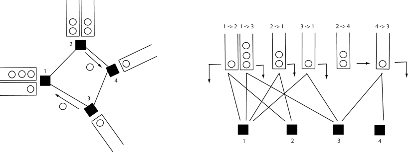
Figure 4: Example of a wireless network with primary interference constraints with four nodes $\{1,2,3,4\}$ and five paths $\{1\to 2,2\to 1,1\to 3,3\to 1,2\to 4\to 3\}$. There is a buffer on each (directed) edge on each path, i.e., six buffers in total. Unit-size packets arrive at the ingress buffer (i.e., the first node) of each path. In the leftmost diagram, two links $2\to 4$ and $3\to 1$ are transmitting (unit-sized) packets. Once a packet is transmitted, it leaves the network if it arrives at the destination node (i.e., the last node on its path). The rightmost diagram illustrates the corresponding stochastic processing network, where the relation between buffers, activities and processors induces a hypergraph (each buffer requires two processors)

.

Necessary condition for stability.

As in the parallel server networks, one can obtain the following necessary condition to stabilize a stochastic processing network satisfying Assumption B1: for all $k\in\mathcal{K}$,

$$\rho^{(k)}:=\sum_{i\in\mathcal{I}:k\in\mathcal{K}_{i}}\rho_{i}~{}<~{}1.$$ (17)

This is because Assumption B1 implies that each buffer has at most one associated activity, and the processing rate is $1$.

Local Lyapunov function.

We consider the following local Lyapunov function:

$$\mathcal{L}_{\mathrm{local}}(x)=\sum_{i\in\mathcal{I}}\sum_{k\in\mathcal{K}_{i}}\sum_{\ell\in\mathcal{I}:k\in\mathcal{K}_{\ell}}x_{i}x_{\ell},\qquad\mbox{for}~{}~{}x=(x_{1},\dots,x_{I}).$$

We now proceed toward proving that condition (3) holds. For given vectors $\boldsymbol{w}=[w_{i}]\in\mathbb{R}_{+}^{I}$ and $\boldsymbol{u}=[u_{j}]\in\mathcal{M}(\boldsymbol{w})$, maximality implies that

$$\sum_{k\in\mathcal{K}_{i}}\sum_{\ell\in\mathcal{I}:k\in\mathcal{K}_{\ell}}u_{\ell}~{}\geq~{}{\bf 1}^{+}_{w_{i}}.$$

Thus, we have that, on writing $\nu_{i}=\rho_{i}+\varepsilon m_{i}$,

$$\mathcal{L}_{\mathrm{local}}(\boldsymbol{w}+\boldsymbol{\rho}+\varepsilon\boldsymbol{m}-s(\boldsymbol{u}))-\mathcal{L}_{\mathrm{local}}(\boldsymbol{w}) \leq \mathcal{C}+2\sum_{i\in\mathcal{I}}w_{i}\left(\sum_{k\in\mathcal{K}_{i}}\sum_{\ell\in\mathcal{I}:k\in\mathcal{K}_{\ell}}\nu_{\ell}-\sum_{k\in\mathcal{K}_{i}}\sum_{\ell\in\mathcal{I}:k\in\mathcal{K}_{\ell}}u_{\ell}\right)$$

$$\leq \mathcal{C}+2\sum_{i\in\mathcal{I}}w_{i}\left(\sum_{k\in\mathcal{K}_{i}}\sum_{\ell\in\mathcal{I}:k\in\mathcal{K}_{\ell}}\nu_{\ell}-{\bf 1}^{+}_{w_{i}}\right)$$

$$= \mathcal{C}+2\sum_{i\in\mathcal{I}}w_{i}\left(\sum_{k\in\mathcal{K}_{i}}\sum_{\ell\in\mathcal{I}:k\in\mathcal{K}_{\ell}}\nu_{\ell}-1\right),$$

where $\mathcal{C}$ is some constant. Therefore, (3) holds if $\nu^{(k)}:=\sum_{i\in\mathcal{I}:k\in\mathcal{K}_{i}}\nu_{i}<\frac{1}{\max_{i\in\mathcal{I}}|\mathcal{K}_{i}|}$ for all $k\in\mathcal{K}$. This is equivalent to

$$0\leq\varepsilon<\min_{k\in\mathcal{K}}\frac{\frac{1}{\max_{i\in\mathcal{I}}|\mathcal{K}_{i}|}-\rho^{(k)}}{m^{(k)}},$$

where we define $m^{(k)}:=\sum_{i\in\mathcal{I}:k\in\mathcal{K}_{i}}m_{i}$. The above interval is non-empty as long as $\rho^{(k)}<\frac{1}{\max_{i\in\mathcal{I}}|\mathcal{K}_{i}|}$ for all $k\in\mathcal{K}$.

Stability of LRFS policies.

We now state the main result for synchronized stochastic networks satisfying Assumption B1. Since the network is synchronized, we obtain the following proposition as a corollary of Theorem 3.5.

Proposition 5.2.

If a stochastic processing network is synchronized and satisfies Assumption B1 with $\rho^{(k)}<\frac{1}{\max_{i\in\mathcal{I}}|\mathcal{K}_{i}|}$ for all $k\in\mathcal{K}$, then

• The $\varepsilon$-LRFS process is queue-length-stable for any $\varepsilon\in\left(0,\min_{k\in\mathcal{K}}\frac{\frac{1}{\max_{i\in\mathcal{I}}|\mathcal{K}_{i}|}-\rho^{(k)}}{m^{(k)}}\right).$

• The LRFS process is queue-length-stable if all routes are bounded in length.

Proposition 5.2 implies that the $\varepsilon$-LRFS policy can achieve a $\frac{1}{\max_{i\in\mathcal{I}}|\mathcal{K}_{i}|}$ fraction of the capacity region (17). For networks of input-queued switches [18, 6] and wireless networks with primary interference constraints [21], it is easy to see that $\max_{i\in\mathcal{I}}|\mathcal{K}_{i}|=2$, and hence the $\varepsilon$-LRFS policy achieves 50% of the capacity region. For wireless networks with general independent set constraints [22], $\max_{i\in\mathcal{I}}|\mathcal{K}_{i}|$ is the maximum number of interfering neighbors, i.e., the maximum degree of the underlying interference graph.

In large-scale networks, distributed scheduling schemes with low complexity have gained much attention recently, even though they usually perform worse than centralized ones with high complexity. We remark that the 50% throughput result of a greedy scheduling algorithm has previously been established for input-queued switches (i.e., no routing between buffers) by Dai et al. [6]. Proposition 5.2 generalizes this to ‘networks’ of input-queued switches operated under stochastic routing between buffers (or local switches). In wireless networks with primary interference constraints, Wu et al. [25] establish the 50% throughput result of the LRFS policy assuming deterministic routing (i.e., fixed routes between nodes), while Proposition 5.2 allows stochastic routing.

6 Proof of Theorem 3.5

To prove the desired stability of the $\varepsilon$-LRFS process $\{X(t)\}$, we construct a new process $\{Y(t)\}$, which is almost identical to $\{X(t)\}$, but it has a larger state space. The main idea of the proof is to construct a Lyapunov function for the ‘larger’ process $\{Y(t)\}$, which implies the stability of $\{Y(t)\}$ and therefore the stability of $\{X(t)\}$.

The description of $\{Y(t)\}$ is as follows. Consider the stochastic processing network setup in Section 2, and let $\mathcal{P}=\{P_{1},P_{2},\dots\}$ be the collection of all possible paths of buffers (allowing repetitions) of length at most $D$ (i.e., $|\mathcal{P}|\leq(I+1)^{D}$), where $D\in\mathbb{N}$ is some finite constant to be determined later. We assume that when a job enters the network, it pre-determines the first $D$ buffers on its route. After being processed from these $D$ buffers, jobs perform the usual stochastic routing as described in Section 2. Let $i_{nm}\in\mathcal{I}$, $Q_{nm}(t)\in\mathbb{Z}_{+}$ and $V_{nm}^{j}(t)\in\mathbb{R}_{+}$ denote the $m$-th buffer on path $P_{n}$, the number of jobs waiting in buffer $i_{nm}$ and the remaining service requirement of the job in buffer $i_{nm}$ being processed by activity $j$ at time $t$, respectively. If activity $j$ is not processing a job in buffer $i_{nm}$, then $V_{nm}^{j}(t)=0$. Furthermore, as before, let $Q_{i,c}(t)$ be the queue length (i.e., the number of jobs waiting for service, excluding those being processed) with counter $c$ in buffer $i$ at time $t$. $V_{i,c}^{j}(t)$ is defined to be the remaining service requirement of the job with counter $c$ in buffer $i$ being processed by activity $j$ at time $t$. We then define

$$Y(t) = \left[Q_{nm}(t),Q_{i,c}(t),V_{nm}^{j}(t),V_{i,c}^{j}(t),\mathcal{T}^{(h)}(t)\right]\in\Omega_{Y}:=\mathbb{Z}_{+}^{\infty}\times\mathbb{R}_{+}^{\infty}\times[0,1]^{H},$$

where $n,m,c,h$ are positive integers such that $n\leq(I+1)^{D}$, $m\leq D$, $c>D$ and $h\leq H$.

As for $\{X(t)\}$, we impose the convention that $\{Y(t)\}$ has right-continuous sample paths. We define the norm $|Y(t)|$ through

$$|Y(t)|~{}=~{}\sum_{n\leq(I+1)^{D},m\leq D}Q_{nm}(t)+\sum_{i\in\mathcal{I},c>D}Q_{i,c}(t)+\sum_{n\leq(I+1)^{D},m\leq D,j\in\mathcal{J}}V^{j}_{nm}(t)+\sum_{i\in\mathcal{I},c>D,j\in\mathcal{J}}V^{j}_{i,c}(t).$$

One can define a natural projection $P$ such that the distribution of $P(Y(t))$ is identical to that of $X(t)$ and $|P(Y(t))|=|X(t)|$ given that $Y(0)$ is drawn appropriately from the preimage $P^{-1}(X(0))$ of $X(0)$. Intuitively speaking, $\{Y(t)\}$ tosses random coins to determine routes in advance, and since the scheduling decisions of $\varepsilon$-LRFS are independent of these coins, the natural projection of $\{Y(t)\}$ ignoring these pre-determined coin flips provides exactly the dynamics of $\{X(t)\}$. Hence, it suffices to prove that the (bigger) process $\{Y(t):t\in\mathbb{R}_{+}\}$ is queue-length-stable, i.e.,

$$\limsup_{t\to\infty}\frac{1}{t}\int_{0}^{t}E\left[|Y(s)|\right]ds<\infty,$$ (18)

for any given initial state $Y(0)\in\Omega_{Y}^{*}:=\{Y\in\Omega_{Y}:|Y|<\infty\}$. In essence, this follows from the following proposition, which is proved in Section 6.1.

Proposition 6.1.

If the conditions of Theorem 3.5 hold, then there exist constants $N,T,D,\zeta,\mathcal{C}\in(0,\infty)$ and a Lyapunov function $\mathcal{L}_{\text{\em global}}:\Omega_{Y}\to\mathbb{R}_{+}\cup\{\infty\}$ such that for all $t\geq N$,

$$E\left[\mathcal{L}_{\text{\em global}}(Y(t+T))~{}|~{}\mathcal{F}(t)\right] \leq \mathcal{L}_{\text{\em global}}(Y(t))-\zeta|Y(t)|+\mathcal{C},\qquad\mbox{almost surely},$$

and $\sup_{Y\in\Omega_{Y}^{*}}{\mathcal{L}_{\text{\em global}}(Y)}/{\mathcal{|}Y|^{2}}<\infty$, where we define the filtration $\{\mathcal{F}(t):t\geq 0\}$ by

$$\mathcal{F}(t):=\sigma\{Y(s):0\leq s\leq t\}.$$

Now we describe how Proposition 6.1 implies (18), and hence the conclusion of Theorem 3.5. First one can observe that $E\left[|Y(t)|^{2}\right]<\infty$ since $Y(0)\in\Omega_{Y}^{*}$ and we assume bounded second moments on arrivals and service times. Since $\sup_{Y\in\Omega_{Y}^{*}}{\mathcal{L}_{\mathrm{global}}(Y)}/{\mathcal{|}Y|^{2}}<\infty$ from Proposition 6.1, it follows that

$$E\left[\mathcal{L}_{\mathrm{global}}(Y(t+T))\right],E\left[\mathcal{L}_{\mathrm{global}}(Y(t))\right],E\left[|Y(t)|\right]<\infty.$$ (19)

Combining Proposition 6.1 and (19) yields that for all $t\geq N$,

$$E\left[\mathcal{L}_{\mathrm{global}}(Y(t+T))\right]~{}\leq~{}E\left[\mathcal{L}_{\mathrm{global}}(Y(t))\right]-\zeta E\left[|Y(t)|\right]+\mathcal{C}.$$

Therefore, we have that for $t\geq N$,

$$\int^{T+t}_{T+N}E\left[\mathcal{L}_{\mathrm{global}}(Y(s))\right]ds = \int^{t}_{N}E\left[\mathcal{L}_{\mathrm{global}}(Y(s+T))\right]ds$$

$$\leq \int^{t}_{N}E\left[\mathcal{L}_{\mathrm{global}}(Y(s))\right]ds-\zeta\int^{t}_{N}E\left[|Y(s)|\right]ds+\mathcal{C}(t-N),$$

which implies that for $t\geq T+N$,

$$\frac{\zeta}{t-N}\int^{t}_{N}E\left[|Y(s)|\right]ds~{}\leq~{}\mathcal{C}+\frac{1}{t-N}\int^{T+N}_{N}E\left[\mathcal{L}_{\mathrm{global}}(Y(s))\right]ds.$$

The right-hand side of the above inequality converges to $\mathcal{C}$ as $t\to\infty$. This leads to the desired conclusion (18).

6.1 Proof of Proposition 6.1

The choice of $N$ in Proposition 6.1 comes from our assumption on the external arrival processes in Section 2, namely, that there exists some $N<\infty$ such that for all $i\in\mathcal{I}$ and $t\geq N$,

$$E\Big{[}A_{i}(t,t+1)~{}\big{|}~{}\{A_{1}(0,s),\dots,A_{I}(0,s):0\leq s\leq t\}\Big{]}~{}\leq~{}\alpha_{i}.$$

For notational convenience, we assume $N=0$ in the proof of Proposition 6.1. Namely, we assume that for all $t\geq 0$,

$$E\Big{[}A_{i}(t,t+1)~{}\big{|}~{}\mathcal{F}(t)\Big{]}~{}\leq~{}\alpha_{i}<\infty.$$ (20)

All the proof arguments are applicable to the general case $N>0$.

We first define some further notation in Section 6.1.1. The skeleton of the proof of Proposition 6.1 is described in Section 6.1.2, and it uses three key lemmas. The proofs of these lemmas follow.

6.1.1 Notation

The quantities defined below are simple functions of the network state $Y(t)$. We use bold symbols to denote vectors of quantities, e.g., $\boldsymbol{Q}_{c}(t)=[Q_{i,c}(t)]$ and $\boldsymbol{W}_{\leq c}(t)=[W_{i,\leq c}(t)]$.

Queues.

For $c\in\mathbb{N}$, let $Q_{i,c}(t)$, $Q_{i,<c}(t)$ and $Q_{i,\leq c}(t)$ be the number of waiting jobs with counter $c$, $<c$ and $\leq c$ in buffer $i$ at time $t$, respectively. That is, we set

$$Q_{i,c}(t)~{}=~{}\sum_{n=1}^{(I+1)^{D}}Q_{nc}(t)\,I_{\{i\}}(i_{nc})\qquad\mbox{for}~{}~{}c\leq D,$$

$$Q_{i,<c}(t)~{}=~{}\sum_{c^{\prime}=1}^{c-1}Q_{i,c^{\prime}}(t)\qquad Q_{i,\leq c}(t)~{}=~{}\sum_{c^{\prime}=1}^{c}Q_{i,c^{\prime}}(t),$$

where we recall that $I_{\{i\}}(i_{nc})=1$ if $i_{nc}=i$ and $I_{\{i\}}(i_{nc})=0$ otherwise. Furthermore, for $c\leq D$, we let $\widehat{Q}_{i,\leq c}(t)$ be the number of waiting jobs with counter $\leq c$ ‘in or destined for’ buffer $i$ at time $t$. Namely,

$$\widehat{Q}_{i,\leq c}(t) = {Q}_{i,\leq c}(t)+\sum_{n=1}^{(I+1)^{D}}\sum_{m=1}^{c}\sum_{r=m+1}^{c}Q_{nm}(t)\,I_{\{i\}}(i_{nr}),$$

where the first term ‘${Q}_{i,\leq c}(t)$’ and the second term ‘$\sum_{n=1}^{(I+1)^{D}}\cdots$’ on the right-hand side count the numbers of waiting jobs currently in buffer $i$ and destined for buffer $i$, respectively.

Workloads.

Let $V^{j}(t)$ denote the remaining service requirement of the job being processed by activity $j$ at time $t$, and $V_{i}(t)$ the total remaining service requirement of the jobs being processed in buffer $i$ at time $t$ (multiple jobs can be processed from the same buffer by different processors). Similarly, $V_{i,c}(t),V_{i,<c}(t),V_{i,\leq c}(t)$ stands for the total remaining service requirement of jobs with counter $c$, $<c$, $\leq c$ being processed in buffer $i$ at time $t$, respectively. We furthermore define the following quantities:

• if the network is not synchronized,

  $${W}_{i,<c}(t) = m_{i}{Q}_{i,<c}(t)+V_{i}(t)$$

  $${W}_{i,\leq c}(t) = m_{i}{Q}_{i,\leq c}(t)+V_{i}(t)$$

  $$\widehat{W}_{i,\leq c}(t) = m_{i}\widehat{Q}_{i,\leq c}(t)+V_{i}(t).$$

• if the network is synchronized,

  $${W}_{i,<c}(t) = m_{i}{Q}_{i,<c}(t)+V_{i,<c}(t)$$

  $${W}_{i,\leq c}(t) = m_{i}{Q}_{i,\leq c}(t)+V_{i,\leq c}(t)$$

  $$\widehat{W}_{i,\leq c}(t) = m_{i}\widehat{Q}_{i,\leq c}(t)+V_{i,\leq c}(t).$$

We use different definitions for these variables depending on whether the network is synchronized or not, since the strategy of the proof differs in each case, e.g., see Section 6.1.4. We also note that in a synchronized network, $V_{i,c}(t),V_{i,<c}(t),V_{i,\leq c}(t)\in\{0,1\}$ for $t\in\mathbb{Z}_{+}$. The quantities $W_{i,<c}(t)$ and $W_{i,\leq c}(t)$ are (expected) immediate workloads, since they only involve work that is in buffer $i$ at time $t$. The quantities $\widehat{W}_{i,\leq c}(t)$ are (expected) total workloads, since they incorporate work currently in the system which will be routed to buffer $i$, regardless where the work resides in the network at time $t$.

Three types of jobs & weights.

We distinguish three types of jobs:

• • Jobs with counter $>D$

  • Jobs on a path of length $=D$ in $\mathcal{P}$.

  • Jobs on a path of length $<D$ in $\mathcal{P}$.

Hence, the counters of jobs of Type 2 and 3 cannot exceed $D$. We further note that each job (regardless whether it is currently being processed or not) can compute its expected total remaining service requirement in the future (under the network process $\{Y(t)\}$), and we call this quantity the weight of the job. Namely, if a job is not currently being processed, its weight is

$$\sum_{i\in\mathcal{I}}m_{i}\,E\big{[}\mbox{the number of times it visits buffer $i$ before it leaves the network}\big{]},$$

which includes the current buffer of the job. Thus, the weight of a waiting job, not currently being processed, can be calculated as follows.

• • The weight of a waiting job of Type 1 in buffer $i\in\mathcal{I}$ is

    $${\bf e}_{i}^{T}(I+P+P^{2}+\cdots)\boldsymbol{m}~{}=~{}{\bf e}_{i}^{T}(I-P)^{-1}\boldsymbol{m},$$

    where $\boldsymbol{m}=[m_{i}]\in\mathbb{R}_{+}^{I}$ and ${\bf e}_{i}\in\{0,1\}^{I}$ is the unit vector with zeros except for its $i$-th coordinate which equals to one (both are column vectors).

  • The weight of a waiting job of Type 2 in buffer $i_{nm}$ on a path $P_{n}$ of length $D$ (i.e., $|P_{n}|=D$) is

    $${\bf e}_{i_{nD}}^{T}(P+P^{2}+P^{3}+\cdots)\boldsymbol{m}+\sum_{k=m}^{D}m_{i_{nk}}~{}=~{}{\bf e}_{i_{nD}}^{T}P(I-P)^{-1}\boldsymbol{m}+\sum_{k=m}^{D}m_{i_{nk}},$$

    where we note that $i_{nD}$ is the last buffer on $P_{n}$.

  • The weight of a waiting job of Type 3 in buffer $i_{nm}$ on a path $P_{n}$ of length $<D$ is

    $$\sum_{k=m}^{|P_{n}|}m_{i_{nk}}.$$

On the other hand, for jobs currently being processed, each weight is calculated as

the current remaining service requirement

$$\qquad+\sum_{i\in\mathcal{I}}m_{i}\,E\big{[}\mbox{the number of times it visits buffer $i$ before it leaves the network}\big{]},$$

where the latter number does not include the current buffer of the job. Now let $M_{1}(t)$, $M_{2}(t)$ and $M_{3}(t)$ be the total weights of jobs of Type 1, 2 and 3 at time $t$, respectively. These total weights are fully determined by the network state information $Y(t)$:

$$M_{1}(t) = \sum_{i\in\mathcal{I},c>D}Q_{i,c}(t)\,{\bf e}_{i}^{T}(I-P)^{-1}\boldsymbol{m}+\sum_{i\in\mathcal{I},c>D,j\in\mathcal{J}}{\bf 1}^{+}_{V^{j}_{i,c}(t)}\left[V^{j}_{i,c}(t)+{\bf e}_{i}^{T}P(I-P)^{-1}\boldsymbol{m}\right],$$

$$M_{2}(t) = \sum_{n\leq(I+1)^{D},m\leq D:|P_{n}|=D}Q_{nm}(t)\left[{\bf e}_{i_{nD}}^{T}P(I-P)^{-1}\boldsymbol{m}+\sum_{k=m}^{D}m_{i_{nk}}\right]$$

$$\quad+\sum_{n\leq(I+1)^{D},m\leq D,j\in J:|P_{n}|=D}{\bf 1}^{+}_{V^{j}_{nm}(t)}\left[V^{j}_{nm}(t)+{\bf e}_{i_{nD}}^{T}P(I-P)^{-1}\boldsymbol{m}+\sum_{k=m+1}^{D}m_{i_{nk}}\right],$$

$$M_{3}(t) = \sum_{n\leq(I+1)^{D},m\leq D:|P_{n}|<D}\left[Q_{nm}(t)\sum_{k=m}^{|P_{n}|}m_{i_{nk}}\right]$$

$$\qquad+\sum_{n\leq(I+1)^{D},m\leq D,j\in\mathcal{J}:|P_{n}|<D}{\bf 1}^{+}_{V^{j}_{nm}(t)}\left[V^{j}_{nm}(t)+\sum_{k=m+1}^{|P_{n}|}m_{i_{nk}}\right],$$

where we recall that ${\bf 1}^{+}_{x}=1$ if $x>0$, and ${\bf 1}^{+}_{x}=0$ otherwise.

6.1.2 Three Auxiliary Lemmas and Proof of Proposition 6.1

We state and prove the following three key lemmas, which we prove in Section 6.1.3, 6.1.4 and 6.1.5, respectively. To simplify notation, we will use $\mathcal{C}$ to denote a finite constant which only depends on the matrix $Z$ given in Theorem 3.5 or on the predefined network parameters from Section 2. Its precise value can be different from line to line.

Lemma 6.2.

There exists a constant $\mathcal{C}<\infty$ such that for all $t\geq 0$,

$$E\left[\|\boldsymbol{V}(t+1)\|_{2}^{2}~{}|~{}\mathcal{F}(t)\right] \leq \|\boldsymbol{V}(t)\|_{2}^{2}-\beta_{\min}\|\boldsymbol{V}(t)\|_{1}+\mathcal{C},$$

where $\beta_{\min}=\min_{j\in\mathcal{J}}\beta_{j}$.

Lemma 6.3.

Suppose that there exists a symmetric matrix $Z\in\mathbb{R}_{+}^{I\times I}$ such that $\mathcal{L}_{\mathrm{local}}(x)=x^{T}Zx$ is a local Lyapunov function with slack $\varepsilon\geq 0$, and that either Condition C1 or C2$\,{}^{\prime}$ from Theorem 3.5 holds. Then given $D\in\mathbb{N}$, there exist constants $\upsilon,\mathcal{C}=\mathcal{C}(D)\in(0,\infty)$ such that for all $c\leq D$, $t\geq 0$,

$$E\left[\mathcal{L}_{\text{\em local}}\left(\widehat{\boldsymbol{W}}_{\leq c}(t+1)\right)~{}\Big{|}~{}\mathcal{F}(t)\right]$$

$$\leq \mathcal{L}_{\text{\em local}}\left(\widehat{\boldsymbol{W}}_{\leq c}(t)\right)-\upsilon\|{\boldsymbol{Q}}_{\leq c}(t)\|_{1}+\mathcal{C}\left(\|\boldsymbol{V}(t)\|_{1}+\|{\boldsymbol{Q}}_{<c}(t)\|_{1}+1\right).$$

Lemma 6.4.

Consider $\varepsilon>0$. If the network is synchronized or if Condition C2 from Theorem 3.5 holds, then there exist constants $D,T\in\mathbb{N}$ and $\mathcal{C},\gamma_{1},\gamma_{2}\in(0,\infty)$ such that for all $t\geq 0$,

$$E\left[\mathcal{G}(Y(t+T))^{2}~{}|~{}\mathcal{F}(t)\right]~{}\leq~{}\mathcal{G}(Y(t))^{2}-\gamma_{2}\|\boldsymbol{Q}_{>D}(t)\|_{1}+\mathcal{C}\left(\|\boldsymbol{Q}_{\leq D}(t)\|_{1}+\|\boldsymbol{V}(t)\|_{1}+1\right),$$

where $\mathcal{G}(Y(t)):=M_{1}(t)+M_{2}(t)+\gamma_{1}\|\boldsymbol{V}(t)\|_{1}$.

Lemma 6.4 is not needed for the proof of Proposition 6.1 if all routes are bounded. Hence, for networks with bounded routes, $\varepsilon=0$ is allowed and only Condition C2$\,{}^{\prime}$ is needed for the desired stability. The right-hand sides of the inequalities in Lemmas 6.2 – 6.4 provide ‘negative drifts’ on $\|\boldsymbol{V}(t)\|_{1}$, $\|{\boldsymbol{Q}}_{\leq D}(t)\|_{1}$ and $\|{\boldsymbol{Q}}_{>D}(t)\|_{1}$, respectively. By appropriately weighing the functions in these three lemmas, we shall construct an appropriate (global) Lyapunov function $\mathcal{L}_{\mathrm{global}}$. To this end, from Lemma 6.2, we obtain

$$E\left[\|\boldsymbol{V}(t+T)\|_{2}^{2}~{}|~{}\mathcal{F}(t)\right] \leq E\left[\|\boldsymbol{V}(t+T-1)\|_{2}^{2}~{}|~{}\mathcal{F}(t)\right]-\beta_{\min}E\left[\|\boldsymbol{V}(t+T-1)\|_{1}~{}|~{}\mathcal{F}(t)\right]+\mathcal{C},$$ (21)

$$\leq E\left[\|\boldsymbol{V}(t+T-1)\|_{2}^{2}~{}|~{}\mathcal{F}(t)\right]+\mathcal{C}$$

$$\leq E\left[\|\boldsymbol{V}(t+T-2)\|_{2}^{2}~{}|~{}\mathcal{F}(t)\right]+2\mathcal{C}$$

$$\qquad\qquad\dots$$

$$\leq E\left[\|\boldsymbol{V}(t+1)\|_{2}^{2}~{}|~{}\mathcal{F}(t)\right]+(T-1)\mathcal{C}$$

$$\leq \|\boldsymbol{V}(t)\|_{2}^{2}-\beta_{\min}\|\boldsymbol{V}(t)\|_{1}+T\mathcal{C},$$

where $T$ is the constant from Lemma 6.4. We write this inequality as

$$E\left[\frac{1}{\beta_{\min}}\|\boldsymbol{V}(t+T)\|_{2}^{2}\,\Big{|}\,\mathcal{F}(t)\right]~{}\leq~{}\frac{1}{\beta_{\min}}\|\boldsymbol{V}(t)\|_{2}^{2}-\|\boldsymbol{V}(t)\|_{1}+\mathcal{C},$$ (22)

where the constant $\mathcal{C}$ is redefined appropriately. We now argue that, similarly, Lemma 6.3 implies that

$$E\left[\mathcal{L}_{\mathrm{local}}\left(\widehat{\boldsymbol{W}}_{\leq c}(t+T)\right)\,\Big{|}\,\mathcal{F}(t)\right]$$

$$\qquad\qquad\qquad\leq~{}\mathcal{L}_{\mathrm{local}}\left(\widehat{\boldsymbol{W}}_{\leq c}(t)\right)-\upsilon\|{\boldsymbol{Q}}_{\leq c}(t)\|_{1}+\mathcal{C}\left(\|\boldsymbol{V}(t)\|_{1}+\|{\boldsymbol{Q}}_{<c}(t)\|_{1}+1\right),$$ (23)

where $\mathcal{C}$ is some (large) constant which may different from the one in Lemma 6.3. To see why this holds, we use the same argument that led to (21) with the additional observation that, for some constant $\mathcal{C}^{\prime}$,

$$\sup_{s\in\{0,1,\ldots,T\}}\left(E\left[\|\boldsymbol{V}(t+s)\|_{1}~{}|~{}\mathcal{F}(t)\right]-\|\boldsymbol{V}(t)\|_{1}\right) \leq \mathcal{C}^{\prime},$$ (24)

$$\sup_{s\in\{0,1,\ldots,T\}}\left(E\left[\|\boldsymbol{Q}(t+s)\|_{1}~{}|~{}\mathcal{F}(t)\right]-\|\boldsymbol{Q}(t)\|_{1}\right) \leq \mathcal{C}^{\prime}.$$ (25)

Here (24) can be derived along the lines of (21), and (25) follows from (20) and the observation that the change in queue length is majorized by the number of external job arrivals.

We now show that Proposition 6.1 follows from these three lemmas, where the last lemma is not needed if all routes are bounded. We consider the following Lyapunov function $\mathcal{L}_{\mathrm{global}}$:

• If all routes are bounded,

  $$\mathcal{L}_{\mathrm{global}}(Y(t))~{}:=~{}\sum_{c=1}^{D}\left(\frac{\upsilon}{2\mathcal{C}}\right)^{c}\mathcal{L}_{\mathrm{local}}\left(\widehat{\boldsymbol{W}}_{\leq c}(t)\right)+\frac{2\mathcal{C}}{\beta_{\min}}\,\|\boldsymbol{V}(t)\|_{2}^{2},$$

  where we choose $D<\infty$ such that $P^{D}=0$, and $\upsilon$ comes from Lemma 6.3.

• Otherwise,

  $$\mathcal{L}_{\mathrm{global}}(Y(t))~{}:=~{}\sum_{c=1}^{D}\left(\frac{\upsilon}{2\mathcal{C}}\right)^{c}\mathcal{L}_{\mathrm{local}}\left(\widehat{\boldsymbol{W}}_{\leq c}(t)\right)+\frac{2\mathcal{C}}{\beta_{\min}}\,\|\boldsymbol{V}(t)\|_{2}^{2}+\frac{\xi}{2\mathcal{C}}\,\mathcal{G}(Y(t))^{2},$$

  where $\upsilon$ and $D$ is from Lemma 6.3 and 6.4, respectively, $\xi:=\xi(\upsilon,\mathcal{C},D)={\upsilon}\left(\frac{\upsilon}{2\mathcal{C}}\right)^{D}$ and $\mathcal{C}$ is a large enough constant chosen so that it can be used for Lemma 6.4 as well as for (22) and (23).

We focus on proving Proposition 6.1 for the case of unbounded routes, but all arguments go through for the other case. Without loss of generality, we assume that

$$\xi,\upsilon,\gamma_{2}<1<\mathcal{C}.$$

The property $\sup_{Y\in\Omega_{Y}^{*}}{\mathcal{L}_{\mathrm{global}}(Y)}/{\mathcal{|}Y|^{2}}<\infty$ in Proposition 6.1 is readily seen to hold. To derive the negative drift property, we observe that Lemma 6.4 in conjunction with (22) and (23) imply that

$$E\left[\mathcal{L}_{\mathrm{global}}(Y(t+T))-\mathcal{L}_{\mathrm{global}}(Y(t))\,\big{|}\,\mathcal{F}(t)\right]$$

$$\qquad\leq\mathcal{C}^{*}-2\mathcal{C}\|{\boldsymbol{V}}(t)\|_{1}+\sum_{c=1}^{D}\left(\frac{\upsilon}{2\mathcal{C}}\right)^{c}\Big{[}-\upsilon\|{\boldsymbol{Q}}_{\leq c}(t)\|_{1}+\mathcal{C}\|{\boldsymbol{Q}}_{<c}(t)\|_{1}+\mathcal{C}\|{\boldsymbol{V}}(t)\|_{1}\Big{]}$$

$$\qquad\qquad-\frac{\gamma_{2}\xi}{2\mathcal{C}}\|\boldsymbol{Q}_{>D}(t)\|_{1}+\frac{\xi}{2}\left(\|\boldsymbol{Q}_{\leq D}(t)\|_{1}+\|\boldsymbol{V}(t)\|_{1}+1\right)$$

$$\qquad\leq\mathcal{C}^{*}-\mathcal{C}\|{\boldsymbol{V}}(t)\|_{1}+\sum_{c=1}^{D}\left(\frac{\upsilon}{2\mathcal{C}}\right)^{c}\Big{[}-\upsilon\|{\boldsymbol{Q}}_{\leq c}(t)\|_{1}+\mathcal{C}\|{\boldsymbol{Q}}_{<c}(t)\|_{1}\Big{]}$$

$$\qquad\qquad-\frac{\gamma_{2}\xi}{2\mathcal{C}}\|\boldsymbol{Q}_{>D}(t)\|_{1}+\frac{\xi}{2}\left(\|\boldsymbol{Q}_{\leq D}(t)\|_{1}+\|\boldsymbol{V}(t)\|_{1}+1\right),$$

where $\mathcal{C}^{*}$ is some (large enough) constant and we use $\upsilon\leq\mathcal{C}$ for the last inequality. The sum in this expression can be bounded as follows:

$$\sum_{c=1}^{D}\left(\frac{\upsilon}{2\mathcal{C}}\right)^{c}\Big{[}-\upsilon\|{\boldsymbol{Q}}_{\leq c}(t)\|_{1}+\mathcal{C}\|{\boldsymbol{Q}}_{<c}(t)\|_{1}\Big{]}$$

$$= -\upsilon\sum_{c=1}^{D}\left(\frac{\upsilon}{2\mathcal{C}}\right)^{c}\|{\boldsymbol{Q}}_{\leq c}(t)\|_{1}+\frac{\upsilon}{2}\sum_{c=1}^{D}\left(\frac{\upsilon}{2\mathcal{C}}\right)^{c-1}\|{\boldsymbol{Q}}_{<c}(t)\|_{1}$$

$$= -{\upsilon}\left(\frac{\upsilon}{2\mathcal{C}}\right)^{D}\|{\boldsymbol{Q}}_{\leq D}(t)\|_{1}-\left(\upsilon-\frac{\upsilon}{2}\right)\sum_{c=1}^{D-1}\left(\frac{\upsilon}{2\mathcal{C}}\right)^{c}\|{\boldsymbol{Q}}_{\leq c}(t)\|_{1}$$

$$\leq -{\upsilon}\left(\frac{\upsilon}{2\mathcal{C}}\right)^{D}\|{\boldsymbol{Q}}_{\leq D}(t)\|_{1}~{}=~{}-\xi\|{\boldsymbol{Q}}_{\leq D}(t)\|_{1}.$$

After combining the preceding two displays, we obtain the desired negative drift property:

$$E\left[\mathcal{L}_{\mathrm{global}}(Y(t+T))-\mathcal{L}_{\mathrm{global}}(Y(t))\,\big{|}\,\mathcal{F}(t)\right]$$

$$\leq \mathcal{C}^{*}-\mathcal{C}\|{\boldsymbol{V}}(t)\|_{1}-\xi\|{\boldsymbol{Q}}_{\leq D}(t)\|_{1}-\frac{\gamma_{2}\xi}{2\mathcal{C}}\|\boldsymbol{Q}_{>D}(t)\|_{1}+\frac{\xi}{2}\left(\|\boldsymbol{Q}_{\leq D}(t)\|_{1}+\|\boldsymbol{V}(t)\|_{1}+1\right)$$

$$\leq \mathcal{C}^{*}+\frac{\xi}{2}-\frac{\gamma_{2}\xi}{2\mathcal{C}}\left(\|{\boldsymbol{V}}(t)\|_{1}+\|{\boldsymbol{Q}_{\leq D}}(t)\|_{1}+\|{\boldsymbol{Q}_{>D}}(t)\|_{1}\right)$$

$$= \mathcal{C}^{*}+\frac{\xi}{2}-\frac{\gamma_{2}\xi}{2\mathcal{C}}\left(\|{\boldsymbol{V}}(t)\|_{1}+\|{\boldsymbol{Q}}(t)\|_{1}\right),$$

where we use $\xi,\upsilon,\gamma_{2}<1$ and $\mathcal{C}>1$. This completes the proof of Proposition 6.1.

6.1.3 Proof of Lemma 6.2

Recall that $\|\boldsymbol{V}(t)\|_{2}^{2}$ is the sum of squares of the remaining service requirements of jobs being processed by some activity at time $t$, i.e.,

$$\|\boldsymbol{V}(t)\|_{2}^{2}~{}=~{}\sum_{j\in\mathcal{J}}V^{j}(t)^{2}\qquad\mbox{and}\qquad\|\boldsymbol{V}(t)\|_{1}~{}=~{}\sum_{j\in\mathcal{J}}V^{j}(t).$$

On the event $\{V^{j}(t)\leq\beta_{j}\}$, activity $j$ has to restart before time $t+1$ and hence,

$$E\left[V^{j}(t+1)^{2}~{}|~{}\mathcal{F}(t)\right]$$

$$\leq E\left[V^{j}(t+1)^{2}~{}|~{}V^{j}(t+1)>0,\mathcal{F}(t)\right]$$

$$\leq E\left[\Gamma_{i_{j},t+1}^{2}~{}\big{|}~{}V^{j}(t+1)>0,\mathcal{F}(t)\right]$$

$$= E\left[E\left[\Gamma_{i_{j},t+1}^{2}~{}\big{|}~{}V^{j}(t+1)>0,\mathcal{F}(t),J^{(t+1)}\right]~{}\big{|}~{}V^{j}(t+1)>0,\mathcal{F}(t)\right],$$

where we let $\Gamma_{i_{j},t+1}$ denote the service time generated by the job being processed by activity $j$ at time $t+1$ and we write

$$J^{(t+1)}:=t+1-\frac{\Gamma_{i_{j},t+1}-V^{j}(t+1)}{\beta_{j}}\in[t,t+1]$$

for the time when this job starts its service. Note that, again on the event $\{V^{j}(t)\leq\beta_{j}\}$,

$$E\left[\Gamma_{i_{j},t+1}^{2}~{}\big{|}~{}V^{j}(t+1)>0,\mathcal{F}(t),J^{(t+1)}\right]$$

$$= \int^{\infty}_{0}\Pr\left[\Gamma_{i_{j},t+1}^{2}>x~{}\big{|}~{}V^{j}(t+1)>0,\mathcal{F}(t),J^{(t+1)}\right]~{}dx$$

$$= \int^{\infty}_{0}\Pr\left[\Gamma_{i_{j}}^{2}>x~{}\big{|}\Gamma_{i_{j}}>\beta_{j}\left(t+1-J^{(t+1)}\right)\right]~{}dx$$

$$= \int^{\infty}_{0}\frac{\Pr\left[\Gamma_{i_{j}}^{2}>x,\Gamma_{i_{j}}>\beta_{j}\left(t+1-J^{(t+1)}\right)\right]}{\Pr\left[\Gamma_{i_{j}}>\beta_{j}\left(t+1-J^{(t+1)}\right)\right]}~{}dx$$

$$\leq \int^{\infty}_{0}\frac{\Pr\left[\Gamma_{i_{j}}^{2}>x\right]}{\Pr[\Gamma_{i_{j}}>\beta_{j}]}~{}dx$$

$$= \frac{E[\Gamma_{i_{j}}^{2}]}{\Pr[\Gamma_{i_{j}}>\beta_{j}]},$$

where we recall that $\Gamma_{i_{j}}$ stands for a generic service time for buffer $i_{j}$. We have thus established that on $\{V^{j}(t)\leq\beta_{j}\}$,

$$E\left[V^{j}(t+1)^{2}~{}|~{}\mathcal{F}(t)\right] \leq \begin{cases}\frac{E[\Gamma_{i_{j}}^{2}]}{\Pr[\Gamma_{i_{j}}>\beta_{j}]}&\mbox{if}~{}\Pr[\Gamma_{i_{j}}>\beta_{j}]>0\\ ~{}~{}~{}~{}\quad(\beta_{j})^{2}&\mbox{otherwise}\end{cases}.$$ (26)

On the other hand, on the event $\{V^{j}(t)>\beta_{j}\}$,

$$V^{j}(t+1)^{2}~{}=~{}(V^{j}(t)-\beta_{j})^{2}~{}\leq~{}V^{j}(t)^{2}-\beta_{j}V^{j}(t)+\beta_{j}^{2}.$$ (27)

Hence, combining (26) and (27), we find that for some constant $\mathcal{C}<\infty$,

$$E[V^{j}(t+1)^{2}~{}|~{}\mathcal{F}(t)]~{}\leq~{}V^{j}(t)^{2}-\beta_{j}V^{j}(t)+\mathcal{C},$$

which leads to the desired conclusion of Lemma 6.2.

6.1.4 Proof of Lemma 6.3

For notational convenience, we stick to the case $t=0$ in the conclusion of Lemma 6.3. Namely, we show that

$$E\left[\mathcal{L}_{\mathrm{local}}\left(\widehat{\boldsymbol{W}}_{\leq c}(1)\right)~{}\big{|}~{}\mathcal{F}(0)\right] \leq \mathcal{L}_{\mathrm{local}}\left(\widehat{\boldsymbol{W}}_{\leq c}(0)\right)-\upsilon\|{\boldsymbol{Q}}_{\leq c}(0)\|_{1}+\mathcal{C}\left(\|\boldsymbol{V}(0)\|_{1}+\|{\boldsymbol{Q}}_{<c}(0)\|_{1}+1\right).$$

However, all arguments go through for general $t>0$.

Non-synchronized network.

We first consider the case when the network may not be synchronized. The first step in the proof is the observation that the schedule $\boldsymbol{\sigma}(t)$ under the $\varepsilon$-LRFS policy is always maximal with respect to the vector $\boldsymbol{w}=[w_{i}]=\left[m_{i}Q_{i,\leq c}(t)\right]$ for any $c\geq 1$. Consequently, since the local quadratic Lyapunov function $\mathcal{L}_{\mathrm{local}}(x)=x^{T}Zx$ satisfies (3), we obtain that for $t\in[0,1]$,

$$2\sum_{(i,\ell)\in\mathcal{I}\times\mathcal{I}}Z_{i\ell}\,w_{\ell}\left(\rho_{i}+\varepsilon m_{i}-\sum_{j\in\mathcal{J}_{i}}\beta_{j}\sigma_{j}(t)\right)~{}\leq~{}-\eta\|\boldsymbol{w}\|_{1}+\mathcal{C},$$

where we further use the observation that

$$\left(w_{i}+\rho_{i}+\varepsilon m_{i}-\sum_{j\in\mathcal{J}_{i}}\beta_{j}\sigma_{j}(t)\right)\left(w_{\ell}+\rho_{\ell}+\varepsilon m_{\ell}-\sum_{j\in\mathcal{J}_{\ell}}\beta_{j}\sigma_{j}(t)\right)-w_{i}w_{\ell}$$

$$\qquad\leq~{}w_{\ell}\left(\rho_{i}+\varepsilon m_{i}-\sum_{j\in\mathcal{J}_{i}}\beta_{j}\sigma_{j}(t)\right)+w_{i}\left(\rho_{\ell}+\varepsilon m_{\ell}-\sum_{j\in\mathcal{J}_{\ell}}\beta_{j}\sigma_{j}(t)\right)+\mathcal{C}.$$ (28)

We remind the reader that we write $\mathcal{C}$ for a finite constant which may differ from line to line. Since we set $w_{i}=m_{i}Q_{i,\leq c}(t)$, it follows that

$$2\sum_{(i,\ell)\in\mathcal{I}\times\mathcal{I}}Z_{i\ell}\,m_{\ell}Q_{\ell,\leq c}(t)\left(\rho_{i}+\varepsilon m_{i}-\sum_{j\in\mathcal{J}_{i}}\beta_{j}\sigma_{j}(t)\right)~{}\leq~{}-\eta\sum_{i\in I}m_{i}Q_{i,\leq c}(t)+\mathcal{C}.$$

After taking conditional expectations given $\mathcal{F}(0)$ on both sides in the above inequality, we obtain

$$2\sum_{(i,\ell)\in\mathcal{I}\times\mathcal{I}}Z_{i\ell}\,m_{\ell}\cdot E\left[{Q}_{\ell,\leq c}(t)\left(\rho_{i}+\varepsilon m_{i}-\sum_{j\in\mathcal{J}_{i}}\beta_{j}\sigma_{j}(t)\right)~{}\Bigg{|}~{}\mathcal{F}(0)\right]~{}\leq~{}-\eta\sum_{i\in I}m_{i}Q_{i,\leq c}(0)+\mathcal{C},$$

where we use that $E[{Q}_{\ell,\leq c}(t)~{}|~{}\mathcal{F}(0)]\geq{Q}_{\ell,\leq c}(0)-\mathcal{C}^{\prime}$ for $t\in[0,1]$ for some constant $\mathcal{C}^{\prime}$. This can be verified by suppressing any arrivals and letting all activities work, and then using the standard fact from renewal theory that any renewal function is finite. Similarly, we obtain from $E\left[{Q}_{\ell,\leq c}(t)~{}\big{|}~{}\sum_{j\in\mathcal{J}_{i}}\beta_{j}\sigma_{j}(t),\mathcal{F}(0)\right]\geq{Q}_{\ell,\leq c}(0)-\mathcal{C}^{\prime}$ for $t\in[0,1]$ that

$$2\sum_{(i,\ell)\in\mathcal{I}\times\mathcal{I}}Z_{i\ell}\,m_{\ell}{Q}_{\ell,\leq c}(0)\cdot E\left[\rho_{i}+\varepsilon m_{i}-\sum_{j\in\mathcal{J}_{i}}\beta_{j}\sigma_{j}(t)~{}\Bigg{|}~{}\mathcal{F}(0)\right]~{}\leq~{}-\eta\sum_{i\in I}m_{i}Q_{i,\leq c}(0)+\mathcal{C},$$ (29)

where the constant $\mathcal{C}$ again has to be redefined appropriately. We leave this inequality for later use.

The second step in the proof is to bound $E\left[\widehat{W}_{i,\leq c}(1)-\widehat{W}_{i,\leq c}(0)~{}\Big{|}~{}\mathcal{F}(0)\right]$ for fixed $i$. Let $\widehat{A}_{i,\leq c}$ be the number of job arrivals contributing to an increase in $\widehat{Q}_{i,\leq c}(\cdot)$ during the time interval $[0,1)$. Then, one can check that for $\widehat{\boldsymbol{A}}_{\leq c}=\left[\widehat{A}_{i,\leq c}\right]$,

$$E\left[\widehat{\boldsymbol{A}}_{\leq c}~{}\big{|}~{}\mathcal{F}(0)\right]~{}\leq~{}\left(I+P+\dots+P^{c}\right)\boldsymbol{\alpha}~{}\leq~{}\boldsymbol{\lambda},$$

since we assume (20). Define the following quantities.

• ${D}_{i,\leq c}$ and ${D}_{i,>c}$ are the numbers of jobs in buffer $i$ which start their service during the time interval $[0,1)$ and with counter $\leq c$ and $>c$, respectively.

• $R_{i,\leq c}$ and $R_{i,>c}$ are the total amounts of service times generated by jobs contributing to ${D}_{i,\leq c}$ and ${D}_{i,>c}$, respectively, again during the time interval $[0,1)$. We stress that the contribution of each job to these quantities may exceed the service time it receives during the interval $[0,1)$.

• $R_{i,>c}^{(L)}$ are the total amounts of service times generated by jobs contributing to $D_{i,>c}$ due to the LRFS policy (i.e., step 4 in Definition 3.2). In addition, we set $R_{i,>c}^{(M)}=R_{i,>c}-R_{i,>c}^{(L)}$.

Then, we have that

$$\Delta_{i,\leq c}~{}:=~{}\widehat{W}_{i,\leq c}(1)-\widehat{W}_{i,\leq c}(0)~{}=~{}m_{i}\left(\widehat{A}_{i,\leq c}-{D}_{i,\leq c}\right)+R_{i,\leq c}+R_{i,>c}-\sum_{j\in\mathcal{J}_{i}}\int^{1}_{0}\beta_{j}\sigma_{j}(t)\,dt.$$ (30)

Taking conditional expectations given $\mathcal{F}(0)$ on both sides, we obtain

$$E\left[\Delta_{i,\leq c}~{}|~{}\mathcal{F}(0)\right]$$

$$\qquad\leq m_{i}\lambda_{i}+E\left[-m_{i}{D}_{i,\leq c}+R_{i,\leq c}~{}|~{}\mathcal{F}(0)\right]+E\left[R_{i,>c}~{}|~{}\mathcal{F}(0)\right]-E\left[\sum_{j\in\mathcal{J}_{i}}\int^{1}_{0}\beta_{j}\sigma_{j}(t)\,dt~{}\Bigg{|}~{}\mathcal{F}(0)\right]$$

$$\qquad=\rho_{i}+E\left[R_{i,>c}~{}|~{}\mathcal{F}(0)\right]-E\left[\sum_{j\in\mathcal{J}_{i}}\int^{1}_{0}\beta_{j}\sigma_{j}(t)\,dt~{}\Bigg{|}~{}\mathcal{F}(0)\right].$$ (31)

Now we bound $E\left[R_{i,>c}~{}|~{}\mathcal{F}(0)\right]$ in the above inequality, or equivalently $E\left[R_{i,>c}^{(L)}~{}\Big{|}~{}\mathcal{F}(0)\right]+E\left[R_{i,>c}^{(M)}~{}\Big{|}~{}\mathcal{F}(0)\right]$ since $R_{i,>c}=R_{i,>c}^{(M)}+R_{i,>c}^{(L)}$. First, one can check that

$$E\left[R_{i,>c}^{(M)}~{}\Big{|}~{}\mathcal{F}(0)\right]~{}\leq~{}\varepsilon m_{i}.$$

This is because the expected number of jobs in buffer $i$ which start their service during the time interval $[0,1)$ due to step 3-1 of the $\varepsilon$-LRFS policy in Definition 3.2 is at most $\varepsilon$ since each timer $\mathcal{T}^{(h)}(t)$ is zero at most once during this time interval. On the other hand, to bound $E\left[R_{i,>c}^{(L)}~{}\Big{|}~{}\mathcal{F}(0)\right]$, consider activity-interchangeable buffers $\ell$ and $i$ (which includes $\ell=i$). Let $\mathcal{E}_{\ell}$ be the event that every job in the queue $Q_{\ell,\leq c}(0)$ (i.e., jobs with counter $\leq c$ waiting in buffer $\ell$ at time $0$) starts service during the time interval $[0,1]$. One can observe that $R_{i,>c}^{(L)}=0$ on the complementary event $\overline{\mathcal{E}}_{\ell}$. We let

$$N:~{}=~{}\sum_{w=1}^{Q_{\ell,\leq c}(0)-|\mathcal{J}_{\ell}|}\Gamma_{\ell,w},$$

where $\{\Gamma_{\ell,w}\}$ are identical random variables with mean $m_{\ell}$ and variance $\varsigma_{\ell}^{2}<\infty$. We first consider the case when

$$E[N~{}|~{}Q_{\ell,\leq c}(0)]=m_{\ell}(Q_{\ell,\leq c}(0)-|\mathcal{J}_{\ell}|)>\beta_{\max}|\mathcal{J}_{\ell}|.$$ (32)

Since $\mathcal{E}_{\ell}$ occurs only if at least $Q_{\ell,\leq c}(0)-|\mathcal{J}_{\ell}|$ jobs complete their service requirements, we obtain the following on the event that (32) holds:

$$\Pr[\mathcal{E}_{\ell}~{}|~{}\mathcal{F}(0)] \leq \Pr\left[N\leq\beta_{\max}|\mathcal{J}_{\ell}|~{}|~{}\mathcal{F}(0)\right]$$ (33)

$$= \Pr\left[N-E[N~{}|~{}Q_{\ell,\leq c}(0)]\leq\beta_{\max}|\mathcal{J}_{\ell}|-E[N~{}|~{}Q_{\ell,\leq c}(0)]~{}|~{}\mathcal{F}(0)\right]$$

$$\leq \Pr\left[\big{(}N-E[N~{}|~{}Q_{\ell,\leq c}(0)]\big{)}^{2}\geq\big{(}E[N~{}|~{}Q_{\ell,\leq c}(0)]-\beta_{\max}|\mathcal{J}_{\ell}|\big{)}^{2}~{}|~{}\mathcal{F}(0)\right]$$

$$\leq \frac{\varsigma_{\ell}^{2}(Q_{\ell,\leq c}(0)-|\mathcal{J}_{\ell}|)}{\big{(}E[N~{}|~{}Q_{\ell,\leq c}(0)]-\beta_{\max}|\mathcal{J}_{\ell}|\big{)}^{2}}$$

$$= \frac{\varsigma_{\ell}^{2}(Q_{\ell,\leq c}(0)-|\mathcal{J}_{\ell}|)}{\big{(}m_{\ell}(Q_{\ell,\leq c}(0)-|\mathcal{J}_{\ell}|)-\beta_{\max}|\mathcal{J}_{\ell}|\big{)}^{2}}$$

$$\leq \frac{\mathcal{C}}{Q_{\ell,\leq c}(0)+1},$$

where $\beta_{\max}=\max_{j\in\mathcal{J}}\beta_{j}$, $\mathcal{C}$ is some (finite) constant depending on $\varsigma_{\ell},m_{\ell},|\mathcal{J}_{\ell}|$ and we use Markov’s inequality in conjunction with (32). On the event that (32) does not hold, i.e., when $Q_{\ell,\leq c}(0)$ is bounded above by $|\mathcal{J}_{\ell}|\left(\beta_{\max}+\frac{1}{m_{\ell}}\right)$, one can redefine the constant $\mathcal{C}$ so that (33) holds. Hence, (33) always holds.

Using (33), it follows that

$$E[R_{i,>c}~{}|~{}\mathcal{F}(0)] = E\left[R_{i,>c}^{(M)}~{}\Big{|}~{}\mathcal{F}(0)\right]+E\left[R_{i,>c}^{(L)}~{}\Big{|}~{}\mathcal{F}(0)\right]$$

$$\leq \varepsilon m_{i}+\Pr[\mathcal{E}_{\ell}~{}|~{}\mathcal{F}(0)]\cdot E\left[R_{i,>c}^{(L)}~{}\big{|}~{}\mathcal{E}_{\ell},\mathcal{F}(0)\right]$$

$$\leq \varepsilon m_{i}+\frac{\mathcal{C}}{Q_{\ell,\leq c}(0)+1}\cdot E\left[R_{i,>c}^{(L)}~{}\big{|}~{}\mathcal{E}_{\ell},\mathcal{F}(0)\right]$$

$$\leq \varepsilon m_{i}+\frac{\mathcal{C}}{Q_{\ell,\leq c}(0)+1},$$

where the last inequality requires that the constant $\mathcal{C}$ has to be redefined appropriately, since $E\left[R_{i,>c}^{(L)}~{}\big{|}~{}\mathcal{E}_{\ell},\mathcal{F}(0)\right]\leq\mathcal{C}^{\prime}$ as can be seen using arguments similar to those leading up to (26). Together with (31), this leads to

$$E\left[\Delta_{i,\leq c}~{}|~{}\mathcal{F}(0)\right] \leq \rho_{i}+\varepsilon m_{i}+\frac{\mathcal{C}}{Q_{\ell,\leq c}(0)+1}-E\left[\sum_{j\in\mathcal{J}_{i}}\int^{1}_{0}\beta_{j}\sigma_{j}(t)\,dt~{}\Bigg{|}~{}\mathcal{F}(0)\right],$$ (34)

for any activity-interchangeable buffers $\ell$ and $i$.

The third step in the proof for the non-synchronized case is to prove the conclusion of Lemma 6.3. By a similar argument as in (28), the claim follows with $\upsilon=\eta\min_{i\in\mathcal{I}}m_{i}$ after we show that

$$2\sum_{(i,\ell)\in\mathcal{I}\times\mathcal{I}}Z_{i\ell}\,\widehat{W}_{\ell,\leq c}(0)\,E[\Delta_{i,\leq c}~{}|~{}\mathcal{F}(0)]~{}\leq~{}-\eta\sum_{i\in\mathcal{I}}m_{i}{Q}_{i,\leq c}(0)+\mathcal{C}\sum_{i\in\mathcal{I}}\Big{[}V_{i}(0)+{Q}_{i,<c}(0)+1\Big{]},$$ (35)

where we use that

$$E\left[\Delta_{i,\leq c}\Delta_{\ell,\leq c}~{}|~{}\mathcal{F}(0)\right]~{}\leq~{}\mathcal{C}$$ (36)

for all $i,\ell$ and some constant $\mathcal{C}$. To see that (36) holds, it suffices to show that $E\left[\Delta_{i,\leq c}^{2}~{}|~{}\mathcal{F}(0)\right]\leq\mathcal{C}$ by the Cauchy-Schwarz inequality. This can be shown using (30) and

$$E\left[\widehat{A}_{i,\leq c}^{2}~{}\big{|}~{}\mathcal{F}(0)\right],E\left[D_{i,\leq c}^{2}~{}|~{}\mathcal{F}(0)\right],E\left[R_{i}^{2}~{}|~{}\mathcal{F}(0)\right]~{}\leq~{}\mathcal{C}$$

where these bounds can be derived using arguments similar to those leading up to (26). Since $Z_{i\ell},E[\Delta_{i,\leq c}~{}|~{}\mathcal{F}(0)]\leq\mathcal{C}$ and

$$\widehat{W}_{\ell,\leq c}(0)~{}\leq~{}{W}_{\ell,\leq c}(0)+\sum_{i\in\mathcal{I}}m_{i}{Q}_{i,<c}(0)~{}=~{}m_{\ell}{Q}_{\ell,\leq c}(0)+V_{\ell}(0)+\sum_{i\in\mathcal{I}}m_{i}{Q}_{i,<c}(0),$$

the inequality in (35) reduces to

$$2\sum_{(i,\ell)\in\mathcal{I}\times\mathcal{I}}Z_{i\ell}\,m_{\ell}{Q}_{\ell,\leq c}(0)\,E[\Delta_{i,\leq c}~{}|~{}\mathcal{F}(0)]~{}\leq~{}-\eta\sum_{i\in\mathcal{I}}m_{i}{Q}_{i,\leq c}(0)+\mathcal{C}.$$ (37)

We prove this using (29) and (34) in conjuction with Condition C2$\,{}^{\prime}$ as follows:

$$2\sum_{(i,\ell)\in\mathcal{I}\times\mathcal{I}}Z_{i\ell}\,m_{\ell}{Q}_{\ell,\leq c}(0)\,E[\Delta_{i,\leq c}~{}|~{}\mathcal{F}(0)]$$

$$\qquad\leq~{}2\sum_{(i,\ell)\in\mathcal{I}\times\mathcal{I}}Z_{i\ell}\,m_{\ell}{Q}_{\ell,\leq c}(0)\left(\rho_{i}+\varepsilon m_{i}+\frac{\mathcal{C}}{Q_{\ell,\leq c}(0)+1}-E\left[\sum_{j\in\mathcal{J}_{i}}\int^{1}_{0}\beta_{j}\sigma_{j}(t)\,dt~{}\Bigg{|}~{}\mathcal{F}(0)\right]\right)$$

$$\qquad\leq~{}2\sum_{(i,\ell)\in\mathcal{I}\times\mathcal{I}}Z_{i\ell}\,m_{\ell}{Q}_{\ell,\leq c}(0)\left(\rho_{i}+\varepsilon m_{i}-E\left[\sum_{j\in\mathcal{J}_{i}}\int^{1}_{0}\beta_{j}\sigma_{j}(t)\,dt~{}\Bigg{|}~{}\mathcal{F}(0)\right]\right)+\mathcal{C}$$

$$\qquad\leq~{}-\eta\sum_{i\in\mathcal{I}}m_{i}{Q}_{i,\leq c}(0)+\mathcal{C},$$

where we again remind the reader that the constant $\mathcal{C}$ may differ from line to line. This completes the proof of Lemma 6.3 for non-synchronized networks.

Synchronized network.

Now we consider the case when the network is synchronized, i.e., Condition C1. We establish the same three steps as in the non-synchronized case. In the non-synchronized case, we used the fact that the schedule $\boldsymbol{\sigma}(t)$ under the $\varepsilon$-LRFS policy is maximal with respect to $[m_{i}Q_{i,\leq c}(t)]$, for which we required Condition C2$\,{}^{\prime}$. In synchronized networks, as a first step in the proof, we use a different (stronger) maximality property, which allows us to relax Condition C2$\,{}^{\prime}$ to Condition C1. To this end, we introduce some necessary notation. We let $\sigma_{j,\leq c}(t)=1$ if activity $j$ processes a job with counter $\leq c$ at time $t$ (and $\sigma_{j,\leq c}(t)=0$ otherwise). Since $\sigma_{j,\leq c}(t)=\sigma_{j,\leq c}(\lfloor t\rfloor)$ in synchronized networks, we write $\sigma_{j,\leq c}=\sigma_{j,\leq c}(0)=\sigma_{j,\leq c}(t)$ for $t\in[0,1)$. The main maximality property we use in synchronized networks is that, under the LRFS policy, the schedule $\left[\sigma_{j,\leq c}I_{\mathcal{I}^{(h)}}(i_{j})\right]$ is maximal with respect to $\left[Q_{i,\leq c}(0)I_{\mathcal{I}^{(h)}}(i)\right]$ for each component $\mathcal{I}^{(h)}$. Together with (3), this implies that for every partition $\mathcal{I}^{(h)}$,

$$2\sum_{(i,\ell)\in\mathcal{I}^{(h)}\times\mathcal{I}^{(h)}}Z_{i\ell}\,{Q}_{\ell,\leq c}(0)\,\left(\rho_{i}+\varepsilon m_{i}-\sum_{j\in\mathcal{J}_{i}}E\left[\sigma_{j,\leq c}~{}|~{}\mathcal{F}(0),\mathcal{E}_{\mbox{\tiny LRFS}}^{(h)}\right]\right)~{}\leq~{}-\eta\sum_{i\in\mathcal{I}}{Q}_{i,\leq c}(0)+\mathcal{C},$$ (38)

where we let $\mathcal{E}_{\mbox{\tiny LRFS}}^{(h)}$ denote the event that at time $0$ the $\varepsilon$-LRFS policy for component $\mathcal{I}^{(h)}$ does not select a job for processing through step 3-1 (see its description in Definition 3.2) and all selected jobs are due the LRFS policy in step 4. We stress that in synchronized networks, every processor completes the service requirement of the job it processes at every integer time $t\in\mathbb{Z}_{+}$ and hence $\Pr\left[\mathcal{E}_{\mbox{\tiny LRFS}}^{(h_{j})}\right]=1-\varepsilon$. Inequality (38) is analogous to (29), which concludes the first step in the non-synchronized case.

We proceed with the analog of the second step from the non-synchronized case, i.e., bounding $E\left[\widehat{W}_{i,\leq c}(1)-\widehat{W}_{i,\leq c}(0)~{}|~{}\mathcal{F}(0)\right]$. We stress that the definition of $\widehat{W}_{i,\leq c}(t)$ differs from the one used in non-synchronized networks, see Section 6.1.1. Scheduling decisions are only made at integer time epochs (i.e., $\sigma(t)=\sigma(\lceil t\rceil)$) in synchronized networks, so that

$$E\left[\widehat{W}_{i,\leq c}(1)-\widehat{W}_{i,\leq c}(0)~{}|~{}\mathcal{F}(0)\right] = E\left[\widehat{A}_{i,\leq c}~{}|~{}\mathcal{F}(0)\right]-\sum_{j\in\mathcal{J}_{i}}E\left[\sigma_{j,\leq c}~{}|~{}\mathcal{F}(0)\right]$$

$$\leq \rho_{i}-\sum_{j\in\mathcal{J}_{i}}E\left[\sigma_{j,\leq c}~{}|~{}\mathcal{F}(0)\right],$$

where we again let $\widehat{A}_{i,\leq c}$ be the number of job arrivals contributing to an increase in $\widehat{Q}_{i,\leq c}(\cdot)$ during the time interval $[0,1)$. On writing $\Delta_{i,\leq c}:=\widehat{W}_{i,\leq c}(1)-\widehat{W}_{i,\leq c}(0)$, we have

$$E\left[{\Delta}_{i,\leq c}~{}|~{}\mathcal{F}(0)\right] \leq \rho_{i}-\sum_{j\in\mathcal{J}_{i}}E\left[\sigma_{j,\leq c}~{}|~{}\mathcal{F}(0)\right].$$ (39)

The third step in the proof for the synchronized case is to prove the conclusion of Lemma 6.3. As in (37), it suffices to prove that

$$2\sum_{(i,\ell)\in\mathcal{I}\times\mathcal{I}}m_{\ell}Z_{i\ell}\,{Q}_{\ell,\leq c}(0)\,E[\Delta_{i,\leq c}~{}|~{}\mathcal{F}(0)]~{}\leq~{}-\eta\sum_{i\in\mathcal{I}}m_{i}{Q}_{i,\leq c}(0)+\mathcal{C}.$$

Since $m_{i}=1$ and $V_{i}(0)\leq 1$ in synchronized networks, this reduces to

$$2\sum_{(i,\ell)\in\mathcal{I}\times\mathcal{I}}Z_{i\ell}\,{Q}_{\ell,\leq c}(0)\,E[\Delta_{i,\leq c}~{}|~{}\mathcal{F}(0)]~{}\leq~{}-\eta\sum_{i\in\mathcal{I}}{Q}_{i,\leq c}(0)+\mathcal{C}.$$ (40)

Combining (39) and (40), it suffices to show that

$$2\sum_{(i,\ell)\in\mathcal{I}\times\mathcal{I}}Z_{i\ell}\,{Q}_{\ell,\leq c}(0)\,\left(\rho_{i}-\sum_{j\in\mathcal{J}_{i}}E\left[\sigma_{j,\leq c}~{}|~{}\mathcal{F}(0)\right]\right)~{}\leq~{}-\eta\sum_{i\in\mathcal{I}}{Q}_{i,\leq c}(0)+\mathcal{C}.$$ (41)

For activity $j\in\mathcal{J}$, writing $\mathcal{I}^{(h_{j})}$ for the component of buffer $i_{j}$ (i.e., $i_{j}\in\mathcal{I}^{(h_{j})}$), we have

$$E\left[\sigma_{j,\leq c}~{}|~{}\mathcal{F}(0)\right] \geq \Pr\left[\mathcal{E}_{\mbox{\tiny LRFS}}^{(h_{j})}\right]E\left[\sigma_{j,\leq c}~{}|~{}\mathcal{F}(0),\mathcal{E}_{\mbox{\tiny LRFS}}^{(h_{j})}\right]$$

$$= (1-\varepsilon)E\left[\sigma_{j,\leq c}~{}|~{}\mathcal{F}(0),\mathcal{E}_{\mbox{\tiny LRFS}}^{(h_{j})}\right]$$

$$\geq E\left[\sigma_{j,\leq c}~{}|~{}\mathcal{F}(0),\mathcal{E}_{\mbox{\tiny LRFS}}^{(h_{j})}\right]-\varepsilon.$$

Therefore, (41) follows after arguing that

$$2\sum_{(i,\ell)\in\mathcal{I}\times\mathcal{I}}Z_{i\ell}\,{Q}_{\ell,\leq c}(0)\,\left(\rho_{i}+\varepsilon m_{i}-\sum_{j\in\mathcal{J}_{i}}E\left[\sigma_{j,\leq c}~{}|~{}\mathcal{F}(0),\mathcal{E}_{\mbox{\tiny LRFS}}^{(h_{j})}\right]\right)~{}\leq~{}-\eta\sum_{i\in\mathcal{I}}{Q}_{i,\leq c}(0)+\mathcal{C}.$$

The above inequality follows from (38) and Condition C1. This completes the proof of Lemma 6.3 for synchronized networks.

6.1.5 Proof of Lemma 6.4

For notational convenience, we again restrict attention to the case $t=0$ in the conclusion of Lemma 6.4, namely, we show that for some $D,T,\mathcal{C},\gamma_{1},\gamma_{2}\in(0,\infty)$,

$$E\left[\mathcal{G}(Y(T))^{2}~{}|~{}\mathcal{F}(0)\right]~{}\leq~{}\mathcal{G}(Y(0))^{2}-\gamma_{2}\|\boldsymbol{Q}_{>D}(0)\|_{1}+\mathcal{C}\left(\|\boldsymbol{Q}_{\leq D}(0)\|_{1}+\|\boldsymbol{V}(0)\|_{1}+1\right),$$

where we recall that

$$\mathcal{G}(Y(t))=M_{1}(t)+M_{2}(t)+\gamma_{1}\|\boldsymbol{V}(t)\|_{1}.$$

All arguments are applicable for general $t\geq 0$ as well. First observe that $M(t):=M_{1}(t)+M_{2}(t)$ can only change through the following events for jobs of Type 1 and 2.

• Arrivals. $M(t)$ increases when new external arrivals of Type 2 occur. Note that there are no such external arrivals for Type 1.

• Routing. $M(t)$ may increase or decrease when a job with counter $\geq D$ (i.e., Type 1 or 2) is routed since the weight (i.e., future workload) of a job conditioned on the buffer to which it has been routed is different from the (unconditional) weight before it is routed. However, $M(t)$ does not change when a job with counter $<D$ (i.e., Type 2) is routed since it is routed deterministically.

• Starting Service. $M(t)$ may increase or decrease when a job of Type 1 or 2 begins service, generating its service time at this point. Assuming the job is served from buffer $i$, then $M(t)$ increases if the random service time is larger than its mean $m_{i}$, and decreases otherwise.

• Being in Service. $M(t)$ decreases when a job of Type 1 or 2 is currently being processed.

Now we express $M(t)$ as follows: for $t\in\mathbb{N}$,

$$M(t)~{}=~{}M(0)+M_{\text{arrival}}(t)+M_{\text{routing}}(t)+M_{\text{s-service}}(t)+M_{\text{b-service}}(t),$$

where $M_{\text{arrival}}(t)$, $M_{\text{routing}}(t)$, $M_{\text{s-service}}(t)$ and $M_{\text{b-service}}(t)$ describe the change in $M(t)$ in the time interval $[0,t]$ due to events of new arrivals, routing, starting service and being in service, respectively. Hence,

$$M_{\text{arrival}}(t)\geq 0\qquad\mbox{and}\qquad M_{\text{b-service}}(t)\leq 0.$$

From our definition of the weights, one can further observe that

$$E[M_{\text{routing}}(t)~{}|~{}\mathcal{F}(0)]~{}=~{}0 \qquad E[M_{\text{s-service}}(t)~{}|~{}\mathcal{F}(0)]~{}=~{}0$$

$$E[M_{\text{arrival}}(t)~{}|~{}\mathcal{F}(0)] \leq t\sum_{d=D}^{\infty}d\,m_{\max}\,\|P^{d}\boldsymbol{\alpha}\|_{1},$$ (42)

where we define $m_{\max}:=\max_{i\in\mathcal{I}}m_{i}$.

By appropriately defining constants $\gamma,T,D,\gamma_{1},\gamma_{2}\in(0,\infty)$, we first prove the following.

$$E\left[\mathcal{G}(Y(T))-\mathcal{G}(Y(0))~{}|~{}\mathcal{F}(0)\right]~{}\leq~{}\begin{cases}-\gamma&\mbox{if}~{}\boldsymbol{Q}_{>D}(0)\neq 0\\ ~{}~{}~{}~{}~{}~{}\mathcal{C}&\mbox{otherwise}\end{cases},$$ (43)

for some constant $\mathcal{C}<\infty$. It is not hard to prove (43) for $\boldsymbol{Q}_{>D}(0)=0$, and hence we only provide the proof for $\boldsymbol{Q}_{>D}(0)\neq 0$. Consider the two complementary events: $\|\boldsymbol{V}(0)\|_{1}\geq 2JB_{\text{renewal}}$ and $\|\boldsymbol{V}(0)\|_{1}<2JB_{\text{renewal}}$, where $B_{\text{renewal}}$ is some constant which will be determined later.

First case.

On the event $\{\|\boldsymbol{V}(0)\|_{1}\geq 2JB_{\text{renewal}}\}$, we observe that $\|\boldsymbol{V}(t)\|_{1}=\sum_{j\in\mathcal{J}}V^{j}(t)$ and

$$E\left[V^{j}(T)~{}|~{}\mathcal{F}(0)\right]~{}\leq~{}\begin{cases}V^{j}(0)-\beta_{j}T&\mbox{if}~{}V^{j}(0)>\beta_{j}T\\ \qquad B_{\text{renewal}}&\mbox{otherwise}\end{cases},$$ (44)

where one can find an appropriate constant $B_{\text{renewal}}<\infty$ depending on the variances of the generic service times $\{\Gamma_{i}\}$ using the renewal theory (e.g., $B_{\text{renewal}}=\max_{i\in\mathcal{I}}E[\Gamma_{i}^{2}]/E[\Gamma_{i}]$ from the proof of Proposition 6.2 in [1]). Hence, in case there is no $j\in\mathcal{J}$ satisfying $V^{j}(0)>\beta_{j}T$,

$$E\left[\|\boldsymbol{V}(T)\|_{1}~{}|~{}\mathcal{F}(0)\right] = \sum_{j\in\mathcal{J}}E\left[V^{j}(T)~{}|~{}\mathcal{F}(0)\right]$$ (45)

$$\leq JB_{\text{renewal}}$$

$$\leq \|\boldsymbol{V}(0)\|_{1}-JB_{\text{renewal}},$$

since $\|\boldsymbol{V}(0)\|_{1}\geq 2JB_{\text{renewal}}$. On the other hand, if there exists a $j_{0}\in\mathcal{J}$ satisfying $V^{j_{0}}(0)>\beta_{j_{0}}T$, we have

$$E\left[\|\boldsymbol{V}(T)\|_{1}~{}|~{}\mathcal{F}(0)\right] = \sum_{j\in\mathcal{J}}E\left[V^{j}(T)~{}|~{}\mathcal{F}(0)\right]$$ (46)

$$= E\left[V^{j_{0}}(T)~{}|~{}\mathcal{F}(0)\right]+\sum_{j\in\mathcal{J}\setminus\{j_{0}\}}E\left[V^{j}(T)~{}|~{}\mathcal{F}(0)\right]$$

$$\leq V^{j_{0}}(0)-\beta_{j_{0}}T+\sum_{j\in\mathcal{J}\setminus\{j_{0}\}}\max\left\{V^{j}(0)-\beta_{j}T,B_{\text{renewal}}\right\}$$

$$\leq V^{j_{0}}(0)-\beta_{j_{0}}T+\sum_{j\in\mathcal{J}\setminus\{j_{0}\}}\left(V^{j}(0)+B_{\text{renewal}}\right)$$

$$\leq \|\boldsymbol{V}(0)\|_{1}+JB_{\text{renewal}}-\beta_{\min}T$$

$$\leq \|\boldsymbol{V}(0)\|_{1}-JB_{\text{renewal}},$$

where we use (44) and choose

$$T~{}>~{}\left\lceil\frac{2JB_{\text{renewal}}}{\beta_{\min}}+1\right\rceil.$$ (47)

Therefore, in both (45) and (46), we have

$$E\left[\|\boldsymbol{V}(T)\|_{1}~{}|~{}\mathcal{F}(0)\right]~{}\leq~{}\|\boldsymbol{V}(0)\|_{1}-JB_{\text{renewal}}.$$

Using this, it follows that

$$E[\mathcal{G}(Y(T))-\mathcal{G}(Y(0))~{}|~{}\mathcal{F}(0)] \leq E\left[M(T)-M(0)~{}|~{}\mathcal{F}(0)\right]+\gamma_{1}E\left[\|\boldsymbol{V}(T)\|_{1}-\|\boldsymbol{V}(0)\|_{1}~{}|~{}\mathcal{F}(0)\right]$$

$$\leq E\left[M_{\text{arrival}}(T)~{}|~{}\mathcal{F}(0)\right]-\gamma_{1}JB_{\text{renewal}}$$

$$\leq T\sum_{d=D}^{\infty}d\,m_{\max}\,\|P^{d}\boldsymbol{\alpha}\|_{1}-\gamma_{1}JB_{\text{renewal}}$$

$$\leq -\gamma,$$

where we use (42) and now define $D,\gamma_{1}$ in terms of $\gamma$ as follows:

$$D=D(\gamma):=\min\left\{x\in\mathbb{N}~{}:~{}T\sum_{d=x}^{\infty}d\,m_{\max}\,\|P^{d}\boldsymbol{\alpha}\|_{1}~{}\leq~{}\gamma\right\}\qquad\gamma_{1}=\gamma_{1}(\gamma):=\frac{2\gamma}{JB_{\text{renewal}}}.$$

We specify the value of $\gamma$ at a later stage in the proof. This completes the proof of (43) on the first event $\{\|\boldsymbol{V}(0)\|_{1}\geq 2JB_{\text{renewal}}\}$.

Second case.

Now consider the second event $\{\|\boldsymbol{V}(0)\|_{1}<{2JB_{\text{renewal}}}\}$. From our choice of $T$ in (47), we have

$$\max_{j\in\mathcal{J}}\frac{V^{j}(0)}{\beta_{j}}~{}\leq~{}\frac{\|\boldsymbol{V}(0)\|_{1}}{\beta_{\min}}~{}<~{}\frac{2JB_{\text{renewal}}}{\beta_{\min}}~{}<~{}T-1,$$

which implies that before time $T-1$, all activities have completed serving the jobs they were serving at time $0$ (and they could have worked on other jobs as well). Thus, it follows that

$$E\left[\|\boldsymbol{V}(T)\|_{1}~{}|~{}\mathcal{F}(0)\right]~{}\leq~{}JB_{\text{renewal}}.$$ (48)

Consider a job with the largest counter (and hence, contributing to $\boldsymbol{Q}_{>D}(0)$) at time $0$ and let $\mathcal{I}^{(h_{0})}\subset\mathcal{I}$ be the component the job belongs to. Define the event $\mathcal{E}_{\text{step 3-1}}$ that the $\varepsilon$-LRFS policy executes step 3-1 (see the description of $\varepsilon$-LRFS in Definition 3.2) for this component at least once before time $T-1$. Let $\mathcal{E}_{\text{step 3-1}}^{*}$ be the subevent that the job identified in step 1 of the policy is selected for processing when step 3-1 is carried out for the first time, so that $\Pr[\mathcal{E}_{\text{step 3-1}}^{*}~{}|~{}\mathcal{E}_{\text{step 3-1}}]=\varepsilon$. On the event $\mathcal{E}_{\text{step 3-1}}^{*}$, let the random variable $j^{*}$ denote the activity which is chosen to process this job, and let $X^{*}$ be the associated service time. We then have that $E[X^{*}|j^{*}]=m_{i_{j^{*}}}.$ Observe that

$$E[M_{\text{s-service}}(T)+M_{\text{b-service}}(T)~{}|~{}j^{*},X^{*},\mathcal{E}_{\text{step 3-1}}^{*},\mathcal{F}(0)]$$

$$\qquad\qquad\qquad\qquad\qquad\qquad\leq~{}\begin{cases}-m_{i_{j^{*}}}+X^{*}-\beta_{j^{*}}&\mbox{on the event}~{}\{X^{*}\geq\beta_{j^{*}}\}\\ \quad\qquad-m_{i_{j^{*}}}&\mbox{otherwise}\end{cases}.$$

It thus follows that

$$E[M_{\text{s-service}}(T)+M_{\text{b-service}}(T)~{}\big{|}~{}\mathcal{E}_{\text{step 3-1}}^{*},\mathcal{F}(0)]$$

$$\leq E\left[-m_{i_{j^{*}}}+[X^{*}-\beta_{j^{*}}]_{+}~{}\big{|}~{}\mathcal{E}_{\text{step 3-1}}^{*},\mathcal{F}(0)\right]$$

$$\leq E\left[-m_{i_{j^{*}}}+[X^{*}-\beta_{\min}]_{+}~{}\big{|}~{}\mathcal{E}_{\text{step 3-1}}^{*},\mathcal{F}(0)\right]$$

$$= E\left[E\left[\left.-m_{i_{j^{*}}}+[X^{*}-\beta_{\min}]_{+}~{}\big{|}~{}j^{*},X^{*},\mathcal{E}_{\text{step 3-1}}^{*},\mathcal{F}(0)\right]~{}\right|~{}\mathcal{E}_{\text{step 3-1}}^{*},\mathcal{F}(0)\right]$$

$$\leq \max_{i\in\mathcal{I}}E\left[-m_{i}+[\Gamma_{i}-\beta_{\min}]_{+}\right],$$

where $\Gamma_{i}$ is a generic service time for buffer $i$ and $[x]_{+}=x$ if $x\geq 0$ and $[x]_{+}=0$ otherwise. It is easy to see that $E\left[-m_{i}+[\Gamma_{i}-\beta_{\min}]_{+}\right]<0$ for all $i$ since $E[\Gamma_{i}]=m_{i}>0$ and $\beta_{\min}>0$. Hence, the above inequality implies that

$$E[M_{\text{s-service}}(T)+M_{\text{b-service}}(T)~{}\big{|}~{}\mathcal{E}_{\text{step 3-1}},\mathcal{F}(0)]~{}\leq~{}-\varepsilon\nu,$$ (49)

with

$$\nu:=\min_{i\in\mathcal{I}}E\left[m_{i}-[\Gamma_{i}-\beta_{\min}]_{+}\right]>0.$$

If the network is synchronized or if the second part of Condition C2 of Theorem 3.5 holds, the only way for the event $\mathcal{E}_{\text{step 3-1}}$ not to occur is that there exists a processor (for the component $\mathcal{I}^{(h_{0})}$) processing a job constantly during the entire time interval $[\mathcal{T}^{(h_{0})}(0),T-1]$ (i.e., the job starts service before time $\mathcal{T}^{(h_{0})}(0)$ and is still in service at time $T-1$). Recall that before time $T-1$, every processor completes the service requirement of the job it was processing at time $0$. Hence, in addition to (47), if we choose $T$ to also satisfy

$$T~{}>~{}2\max_{i\in\mathcal{I}}m_{i}+2,$$

then it follows that

$$\Pr[\mathcal{E}_{\text{step 3-1}}~{}|~{}\mathcal{F}(0)]\geq\left(\frac{1}{2}\right)^{K},$$ (50)

where we use the fact that if a processor starts to process a new job in the time interval $(0,\mathcal{T}^{(h_{0})}(0)]\subset(0,1]$, its service requirement is at most $2\max_{i\in\mathcal{I}}m_{i}$ with probability $1/2$ by the Markov inequality. From (49) and (50), we conclude that

$$E[M_{\text{s-service}}(T)+M_{\text{b-service}}(T)~{}|~{}\mathcal{F}(0)]~{}\leq~{}-\frac{\varepsilon\nu}{2^{K}}.$$ (51)

From (42), (48) and (51), the desired inequality (43) follows as

$$E[\mathcal{G}(Y(T))-\mathcal{G}(Y(0))~{}|~{}\mathcal{F}(0)]$$

$$\qquad\leq~{}E\left[M(T)-M(0)~{}|~{}\mathcal{F}(0)\right]+\gamma_{1}E\left[\|\boldsymbol{V}(T)\|_{1}-\|\boldsymbol{V}(0)\|_{1}~{}|~{}\mathcal{F}(0)\right]$$

$$\qquad\leq~{}E\left[M_{\text{arrival}}(T)~{}|~{}\mathcal{F}(0)\right]+E[M_{\text{s-service}}(T)+M_{\text{b-service}}(T)~{}|~{}\mathcal{F}(0)]+\gamma_{1}JB_{\text{renewal}}$$

$$\qquad\leq~{}T\sum_{d=D}^{\infty}d\,m_{\max}\,\|P^{d}\boldsymbol{\alpha}\|_{1}-\frac{\varepsilon\nu}{2^{K}}+\gamma_{1}JB_{\text{renewal}}$$

$$\qquad\leq~{}-\gamma,$$

where for the last inequality we define

$$\gamma~{}:=~{}\frac{\varepsilon\,\nu}{2^{K+2}}.$$

Here we note that $D=D(\gamma)<\infty$ as long as $\gamma>0$ (i.e., $\varepsilon>0$). This completes the proof of (43) on the second event $\{\|\boldsymbol{V}(0)\|_{1}<2JB_{\text{renewal}}\}$.

Completing the proof of Lemma 6.4.

Now (43) implies that

$$E[\mathcal{G}(Y(T))^{2}-\mathcal{G}(Y(0))^{2}~{}|~{}\mathcal{F}(0)] \leq 2\mathcal{G}(Y(0))\,E[\mathcal{G}(Y(T))-\mathcal{G}(Y(0))~{}|~{}\mathcal{F}(0)]+\mathcal{C}$$

$$\leq 2\left(-\gamma{\bf 1}^{+}_{\|\boldsymbol{Q}_{>D}(0)\|_{1}}+\mathcal{C}\left(1-{\bf 1}^{+}_{\|\boldsymbol{Q}_{>D}(0)\|_{1}}\right)\right)\mathcal{G}(Y(0))+\mathcal{C}$$

$$= 2\left(-(\gamma+\mathcal{C}){\bf 1}^{+}_{\|\boldsymbol{Q}_{>D}(0)\|_{1}}+\mathcal{C}\right)\mathcal{G}(Y(0))+\mathcal{C}$$

where one can check $E\left[\left(\mathcal{G}(Y(T))-\mathcal{G}(Y(0))\right)^{2}~{}\big{|}~{}\mathcal{F}(0)\right]<\infty$ for the first inequality and the precise value of $\mathcal{C}$ can be different from line to line. Finally, we define

$$\gamma_{2}:=m_{\min}\gamma$$

and the conclusion of Lemma 6.4 follows from

$$E[\mathcal{G}(Y(T))^{2}-\mathcal{G}(Y(0))^{2}~{}|~{}\mathcal{F}(0)] \leq 2\left(-(\gamma+\mathcal{C}){\bf 1}^{+}_{\|\boldsymbol{Q}_{>D}(0)\|_{1}}+\mathcal{C}\right)\mathcal{G}(Y(0))+\mathcal{C}$$

$$\leq -2\gamma\,m_{\min}\|\boldsymbol{Q}_{>D}(0)\|_{1}+\mathcal{C}\left(\|\boldsymbol{Q}_{\leq D}(0)\|_{1}+\|\boldsymbol{V}(0)\|_{1}+1\right)$$

$$= -\gamma_{2}\|\boldsymbol{Q}_{>D}(0)\|_{1}+\mathcal{C}\left(\|\boldsymbol{Q}_{\leq D}(0)\|_{1}+\|\boldsymbol{V}(0)\|_{1}+1\right),$$

where we use $\mathcal{G}(Y(0))\leq\mathcal{C}\left(\|\boldsymbol{Q}_{\leq D}(0)\|_{1}+\|\boldsymbol{V}(0)\|_{1}+1\right)$ for the case $\boldsymbol{Q}_{>D}(0)=0$ and $\mathcal{G}(Y(0))\geq m_{\min}\|\boldsymbol{Q}_{>D}(0)\|_{1}$ for the other case $\boldsymbol{Q}_{>D}(0)\neq 0$ (i.e., $\|\boldsymbol{Q}_{>D}(0)\|_{1}>0$).

References

- [1] S. Asmussen. Applied probability and queues. Springer Verlag, 2003.
- [2] M. Bramson. Stability of earliest-due-date, first-served queueing networks. Queueing systems, 39(1):79-102, 2001.
- [3] J. G. Dai. On positive Harris recurrence of multiclass queueing networks: a unified approach via fluid limit models. Annals of Applied Probability, 5:49-77, 1995.
- [4] J. G. Dai. Stability of open multiclass queueing networks via fluid models. IMA Workshop on Stochastic Networks, Springer-Verlag, New York, 71-90, 1995.
- [5] J. G. Dai and W. Lin. Asymptotic optimality of maximum pressure policies in stochastic processing networks. Annals of Applied Probability, 18(6):2239-2299, 2008.
- [6] J. G. Dai and B. Prabhakar. The throughput of data switches with and without speedup. IEEE INFOCOM, 556-564, Tel-Aviv, Israel, 2000.
- [7] J. G. Dai and G. Weiss. Stability and instability of fluid models for reentrant lines. Mathematics of Operations Research, 21:115-134, 1996.
- [8] A. B. Dieker and X. Gao. Positive recurrence of piecewise Ornstein-Uhlenbeck processes and common quadratic Lyapunov functions. Arxiv preprint arXiv:1107.2873, 2011.
- [9] P. Dupuis and R. J. Williams. Lyapunov functions for semimartingale reflecting Brownian motions. Annals of Probability, 22:680-702, 1994.
- [10] S. Foss and T. Konstantopoulos. An overview of some stochastic stability methods. Journal of the Operations Research Society of Japan, 47(4):275-303, 2004.
- [11] J. M. Harrison. Heavy traffic analysis of a system with parallel servers: Asymptotic optimality of discrete-review policies. Annals of Applied Probability, 8:822-848, 1998.
- [12] J. M. Harrison. Brownian models of open processing networks: Canonical representation of workload. Annals of Applied Probability, 10:75-103, MR1765204, 2000.
- [13] F. P. Kelly. Stochastic models of computer communication systems. J. R. Statist. Soc B, 47(3):379.395, 1985.
- [14] P. R. Kumar and S. P. Meyn. Stability of queueing networks and scheduling policies. IEEE Transactions on Automatic Control, 40(2):251-260, 1995.
- [15] P. R. Kumar and T. I. Seidman. Dynamic instabilities and stabilization methods in distributed real-time scheduling of manufacturing systems. IEEE Transactions on Automatic Control, 35:289–298, 1990.
- [16] M. Leconte, J. Ni and R. Srikant. Improved Bounds on the Throughput Efficiency of Greedy Maximal Scheduling in Wireless Networks. IEEE/ACM Transactions on Networking, 19(3):709-720, 2011.
- [17] S. H. Lu and P. R. Kumar. Distributed scheduling based on due dates and buffer priorities. IEEE Transactions on Automatic Control, 36:1406–1416, 1991.
- [18] N. McKeown, V. Anantharan and J. Walrand. Achieving 100% throughput in an input-queued switch. IEEE INFOCOM, 296-302, San Francisco, 1996.
- [19] J. Mo and J. Walrand. Fair end-to-end window-based congestion control. IEEE/ACM Transactions on Networking, 8(5):556.567, 2000.
- [20] A. Rybko and A. Stolyar. On the ergodicity of stochastic processes describing open queueing networks. Problemi Peredachi Informatsii, 28:3-26, 1992.
- [21] S. Sanghavi, L. Bui and R. Srikant. Distributed link scheduling with constant overhead. ACM SIGMETRICS Performance Evaluation Review, 35(1):313-324, 2007.
- [22] D. Shah, J. Shin and P. Tetali. Medium Access using Queues. Annual IEEE Symposium on Foundations of Computer Science (FOCS), Palm Springs, California, 2011.
- [23] D. Shah and D. Wischik. Switched networks with maximum weight policies: Fluid approximation and multiplicative state space collapse. To appear in Annals of Applied Probability, Arxiv preprint arXiv:1004.1995, 2010.
- [24] L. Tassiulas and A. Ephremides. Stability properties of constrained queueing systems and scheduling policies for maximum throughput in multihop radio networks. IEEE Transactions on Automatic Control, 37:1936-1948, 1992.
- [25] X. Wu, R. Srikant and J. R. Perkins. Scheduling efficiency of distributed greedy scheduling algorithms in wireless networks. Mobile Computing, IEEE Transactions on, 6(6):595-605, 2007.