Nonequilibrium static growing length scales in supercooled liquids on approaching the glass transition

Abstract

The small wavenumber $k$ behavior of the structure factor $S(k)$ of overcompressed amorphous hard-sphere configurations was previously studied for a wide range of densities up to the maximally random jammed state, which can be viewed as a prototypical glassy state [A. Hopkins, F. H. Stillinger and S. Torquato, Phys. Rev. E, 86, 021505 (2012)]. It was found that a precursor to the glassy jammed state was evident long before the jamming density was reached as measured by a growing nonequilibrium length scale extracted from the volume integral of the direct correlation function $c(r)$, which becomes long-ranged as the critical jammed state is reached. The present study extends that work by investigating via computer simulations two different atomic models: the single-component Z2 Dzugutov potential in three dimensions and the binary-mixture Kob-Andersen potential in two dimensions. Consistent with the aforementioned hard-sphere study, we demonstrate that for both models a signature of the glass transition is apparent well before the transition temperature is reached as measured by the length scale determined from from the volume integral of the direct correlation function in the single-component case and a generalized direct correlation function in the binary-mixture case. The latter quantity is obtained from a generalized Orstein-Zernike integral equation for a certain decoration of the atomic point configuration. We also show that these growing length scales, which are a consequence of the long-range nature of the direct correlation functions, are intrinsically nonequilibrium in nature as determined by an index $X$ that is a measure of deviation from thermal equilibrium. It is also demonstrated that this nonequilibrium index, which increases upon supercooling, is correlated with a characteristic relaxation time scale.

I Introduction

A quantitative understanding of nature of the physics of the glass transition is one of the most fascinating and challenging problems in materials science and condensed-matter physics. A sufficiently rapid quench of a liquid from above its freezing temperature into a supercooled regime can avoid crystal nucleation to produce a glass with a relaxation time that is much larger than experimental time scales, resulting in an amorphous characteristic state (without long-range order) that is simultaneously rigid Chaikin and Lubensky (1995). A question that has received considerable attention in recent years is whether the growing relaxation times under supercooling have accompanying growing structural length scales. Two distinct schools of thought have emerged to address this question. One asserts that static structure of a glass, as measured by pair correlations, is indistinguishable from that of the corresponding liquid. Thus, since there is no signature of increasing static correlation length scales accompanying the glass transition, it identifies growing dynamical length scales. Berthier et al. (2007); Karmakar et al. (2009); Chandler and Garrahan (2010) The other camp contends that there is a static growing length scale of thermodynamic origin Lubchenko and Wolynes (2006); Hocky et al. (2012) and therefore one need not look for growing length scales associated with the dynamics.

In the present paper, we employ both theoretical and computational methods to study two different atomic glass-forming liquid models that support an alternative view, namely, the existence of a growing static length scale as the temperature of the supercooled liquid is decreased that is intrinsically nonequilibrium in nature. This investigation extends recent previous work Ho12 in which this conclusion was first reached by examining overcompressed hard-sphere liquids up to the maximally random jammed (MRJ) state. Torquato et al. (2000) (For a hard-sphere system, compression qualitatively plays the same role as decreasing the temperature in an atomic or molecular system; see Ref. Torquato and Stillinger, 2010.) The MRJ state under the strict-jamming constraint is a prototypical glass in that it lacks any long-range order but is perfectly rigid such that the elastic moduli are unbounded.Torquato and Stillinger (2007, 2010) This endows such packings with the special hyperuniformity attribute. A statistically homogeneous and isotropic single-component point configuration at number density $\rho$ is hyperuniform if its structure factor

$$S(k)=1+\rho{\widetilde{h}}(k)$$ (1)

tends to zero as the wavenumber $k\rightarrow 0$,Torquato and Stillinger (2003) where $h(r)\equiv g_{2}(r)-1$ is the total correlation function, $g_{2}(r)$ is the pair correlation function, and $\widetilde{h}(k)$ is the Fourier transform of $h(r)$. This condition implies that infinite-wavelength density fluctuations vanish.

It was theoretically established that hyperuniform point distributions are at an “inverted” critical point in that the direct correlation function $c(r)$, rather than the total correlation function $h(r)$, becomes long-ranged, i.e., it decays more slowly than $-1/r^{d}$ in $d$-dimensional Euclidean space $\mathbb{R}^{d}$, where $r$ is the radial distance. Torquato and Stillinger (2003) The Fourier transform of direct correlation function ${\widetilde{c}}(k)$ is defined via the Ornstein-Zernike equation: Hansen and McDonald (2006)

$${\widetilde{c}}(k)=\frac{{\widetilde{h}}(k)}{1+\rho{\widetilde{h}}(k)}=\frac{S(k)-1}{\rho S(k)}.$$ (2)

It is immediately clear from this definition that the real-space volume integral of the direct correlation function $c(r)$ diverges to minus infinity for any hyperuniform system, since the denominator of (2) tends to zero, i.e.,

$$\lim_{k\rightarrow 0}{\widetilde{c}}(k)=\int_{{\mathbb{R}}^{d}}c(r)d{\bf r}\rightarrow-\infty$$ (3)

MRJ packings of identical spheres possess a special type of hyperuniformity such that $S(k)$ tends to zero linearly in $k$ as $k\rightarrow 0$, implying quasi-long-ranged negative pair correlations (anticorrelations) in which $h(r)$ decays as a power law $-1/r^{4}$ or, equivalently, a direct correlation function that decays as $c(r)\sim-1/r^{2}$ for large r, as dictated by Eq. (2).Donev et al. (2005a) These anticorrelations reflect an unusual spatial patterning of regions of lower and higher local particle densities relative to the system density. This quasi-long-range behavior of $h(r)$ is distinctly different from typical liquids in equilibrium, which tend to exhibit more rapidly decaying pair correlations, including exponential decays.

Reference Ho12, examined overcompressed hard-sphere configurations that follow Newtonian dynamics for a wide range of densities up to the MRJ state. A central result of this study was to establish that a precursor to the glassy jammed state was evident long before the MRJ density was reached as measured by an associated growing length scale, extracted from the volume integral of the direct correlation function $c(r)$, which of course diverges at the “critical” hyperuniform MRJ state. It was also shown that the nonequilibrium signature of the aforementioned quasi-long-range anticorrelations, which was quantified via a nonequilibrium index $X$, emerges well before the jammed state was reached.

These results for nonequilibrium amorphous hard-sphere packings suggest that the direct correlation function of supercooled atomic models in which the atoms possess both repulsive and attractive interactions should provide a robust nonequilibrium static growing length scale as the temperature is decreased to the glass transition and below. Here we show that this is indeed the case by extracting length scales associated with standard and generalized direct correlation functions. In particular, we study the single-component Z2 Dzugutov potential in three dimensions and the binary-mixture Kob-Andersen potential in two dimensions. The Z2 Dzugutov potential for a single-component many-particle system in three dimensions has the following form:Doye et al. (2003)

$$v(r)=\left\{\begin{array}[]{ll}a\frac{\displaystyle e^{\eta r}}{\displaystyle r^{3}}\cos(2k_{f}r)+b\left(\frac{\displaystyle\sigma}{\displaystyle r}\right)^{n}+V_{0},&\quad r<r_{c},\\ 0,&\quad r\geq r_{c}.\end{array}\right.$$ (4)

The first term in (4) models Friedel oscillations for a metal with Fermi wave vectors of magnitude $k_{F}$, while the second term adds a strong repulsion for sufficiently small interparticle separations. The parameters $a$ and $b$ control the relative strengths of both contributions and define the energy scale. The cutoff $r_{c}$ is selected to be at the third minimum of the potential, while the constant $V_{0}$ is present to make the potential continuous at the cutoff. The parameters $\eta$, $\sigma$, and $n$ control the shapes of both functions in (4). The Kob-Andersen model for a two-dimensional binary mixture is given by a truncated Lennard-Jones potential:Kob and Andersen (1994)

$$v_{\alpha\beta}(r)=\left\{\begin{array}[]{ll}4\epsilon_{\alpha\beta}\left[\left(\displaystyle\frac{\sigma_{\alpha\beta}}{r}\right)^{12}-\left(\displaystyle\frac{\sigma_{\alpha\beta}}{r}\right)^{6}\right]+V_{0\alpha\beta},&\quad r<2.5\sigma_{\alpha\beta},\\ 0,&\quad r\geq 2.5\sigma_{\alpha\beta}.\end{array}\right.$$ (5)

The parameter $\epsilon_{\alpha\beta}$ controls the strength of the attraction between two particles of species $\alpha$ and $\beta$, while $\sigma_{\alpha\beta}$ is equal to $2^{-1/6}$ times the distance between both particles at which the attraction is maximal.

It is known that overcompressing a hard-sphere system is analogous to supercooling a thermal liquid, but to what extent does this analogy hold? Roughly speaking, a rapid densification of a monodisperse hard-sphere system leads to the terminal MRJ state (with packing fraction of about 0.64), which we have noted is a prototypical glass.Torquato and Stillinger (2010) At this singular state, the system is never able to relax and hence the associated relaxation time is infinite.Rintoul1996 Slower densification rates lead to other jammed states with packing fractions higher than 0.64.Torquato and Stillinger (2010) Moreover, it has been shown that below 0.64, metastable hard-sphere systems have bounded characteristic relaxation times,Rintoul1996 ; Schweizer2007 including the range of packing fractions of about $0.58\sim 0.60$ (depending on the densification rate) that has been interpreted to be the onset of a kinetic glass transition.Schweizer2007 Above a particular hard-sphere glass-transition density, the system is able to support a shear stress on time scales small compared to a characteristic relaxation time. Clearly, increasing the density of a hard-sphere system plays the same role as decreasing temperature of a thermal liquid. In a thermal system, a glass at absolute zero temperature has an infinite relaxation time classically, and hence this state is the analog of the hard-sphere MRJ state. The glass transition temperature $T_{g}$, which depends on the quenching rate and possesses a bounded characteristic relaxation time, is analogous to the aforementioned kinetic transition in hard spheres. These strong analogies between glassy hard-sphere states and glassy atomic systems lead one to believe that the results of Ref. Ho12, for the former extend to the latter. Indeed, here we demonstrate that the aforementioned length scales grow as as the temperature is decreased to the glass transition $T_{g}$ and below. Moreover, we show that the nonequilibrium index $X$, previously shownHo12 to increase as a hard-sphere system is densified to the MRJ state, also grows for $T<2.2T_{g}$. This nonequilibrium index is also shown to be correlated with an early relaxation time $\tau$.

In Sec. II, we introduce two generalizations of the direct correlation function $c(r)$ which apply for two-component systems. In Sec. III we describe the numerical techniques and parameters used in our simulations, while in Sec. IV we present the results we extract from these simulations. The latter includes the demonstration of the existence of growing nonequilibrium static length scales upon supercooling the two atomic-liquid models that we consider. Moreover, we show that the nonequilibrium index $X$ is positively correlated with an early relaxation time, both of which increase as the temperature is decreased to the glass transition temperature and below. We conclude in Sec. V with a summary of our results and of their impact.

II Structural Signatures of Large-Wavelength Density Fluctuations in Binary Mixtures

It has been shown that for maximally random jammed binary sphere packings, the standard structure factor $S(k)$, determined from the particle centroids, cannot be used to ascertain whether the system is hyperuniform, unlike the single-component MRJ sphere packing.Zachary et al. (2011); end (c) Instead it was shown that the spectral density $\widetilde{\chi}(k)$, defined below, can be employed to determine whether a binary MRJ packing is hyperuniform, since it vanishes as $k\rightarrow 0$. We will show below that one must modify the spectral density for particles interacting with soft (non-hard-core) pair potentials because particle-shape information is required in order to ascertain whether the system is hyperuniform or nearly hyperuniform. For particles interacting with a hard-core repulsion, the particle shapes are obviously the hard cores, but for non-hard-core interactions, such as in the Kob-Andersen model studied in this paper, one must determine a self-consistent procedure to assign particle shapes to each point particle. In addition, for such soft binary mixtures, the standard direct correlation function $c(r)$, applicable to monodisperse systems, must be generalized.

In this section, we present two generalizations of $c(\mathbf{r})$ for polydisperse systems: one that is based on the spectral density (Sec. II.2.1), and another that is based on the matrix version of the structure factor (Sec. II.2.2).

II.1 Single-Component Ornstein-Zernike Equation

For a statistically homogeneous and isotropic single component system, the Ornstein-Zernike (OZ) equationHansen and McDonald (2006) defines the direct correlation function $c(r)$ in term of the total correlation function $h(r)=g_{2}(r)-1$ and the system point density $\rho$:

$$h(r)=c(r)+\rho h(r)\otimes c(r),$$ (6)

where $\otimes$ denotes a convolution. After taking the Fourier transform of Eq. (6) and introducing the structure factor $S(k)=1+\rho\widetilde{h}(k)$, we get

$$\widetilde{h}(k)=\widetilde{c}(k)+\rho\widetilde{h}(k)\widetilde{c}(k),$$ (7)

which is equivalent to expression (2).

As noted in the introduction, we see from relation (2) that for hyperuniform single-component systems, i.e., $\lim_{k\rightarrow 0}S(k)=0$, $\widetilde{c}(k)$ diverges toward $-\infty$ as $k$ approaches 0.

II.2 Generalization of the Ornstein-Zernike Equation for “Two-Phase” Decorations

As indicated in the beginning of the section, we must obtain a modified version of the direct correlation function for binary mixtures in which the particles interact with non-hard-core pair potentials in order to detect hyperuniformity or near-hyperuniformity. This function must be defined to be as general as possible. In particular, it must be equivalent to the usual direct correlation function in the case of a single-component system. We shall therefore start by determining what this modified function would be in the single-component case in order to provide insight for the more general case of multiple-component systems. This will be done by decorating the underlying point configuration with nonoverlapping spheres. We first describe the single-component case and then the mixture case.

II.2.1 Single-Component Case

Consider a configuration of $N$ points within a large volume $V$ in which the minimum pair separation is the distance $R$. Now let us decorate this configuration by circumscribing spheres of radius $R$ around each of the points, leading to a configuration of $N$ nonoverlapping spheres of radius $R$. In this case, the particle phase indicator $\mathcal{I}(\mathbf{x})$ in terms of the positions of the sphere centers $\mathbf{r}_{1},\mathbf{r}_{2},\ldots,\mathbf{r}_{N}$ is:Torquato1985 ; TorquatoBook

$$\mathcal{I}(\mathbf{x})=\sum_{i=1}^{N}m(|\mathbf{x}-\mathbf{r}_{i}|;R),$$ (8)

where $m(r;R)$ is the single-inclusion indicator function given by

$$m(r;R)\equiv\Theta(R-r)=\left\{\begin{array}[]{ll}1,&\quad r\leq R,\\ 0,&\quad r>R.\end{array}\right.$$ (9)

The two-point correlation function $S_{2}(r)=\langle I({\bf x})I({\bf x}+{\bf r})\rangle$ for such a statistically homogeneous and isotropic distribution of nonoverlapping spheres, equal to the probability of finding two points, separated by the distance $r\equiv|{\bf r}|$, anywhere in the region occupied by the spheres, has been shown to be given by the following sum of two terms:Torquato1985 ; TorquatoBook

$$S_{2}(r)=\rho m(r)\otimes m(r)+\rho^{2}m(r)\otimes g_{2}(r)\otimes m(r)\;,$$ (10)

where $\rho=\lim_{V\rightarrow\infty}N/V$ is the number density and angular brackets denote an ensemble average. The quantity $\rho m\otimes m$ is the self-correlation term, which is equal to the probability of finding two points inside the same sphere, and $\rho^{2}m\otimes g_{2}\otimes m$ is the two-body correlation, the probability of finding two points in two different spheres. The autocovariance function $\chi(r)$ is:

$$\chi(r) \equiv S_{2}(r)-\rho^{2}v_{1}^{2}=\rho m(r)\otimes m(r)+\rho^{2}m(r)\otimes g_{2}(r)\otimes m(r)-\rho^{2}v_{1}^{2},$$ (11)

$$= \rho m(r)\otimes m(r)+\rho^{2}m(r)\otimes h(r)\otimes m(r),$$

where

$$v_{1}(R)=\int m(r;R)d\mathbf{r}=\frac{\pi^{\frac{d}{2}}R^{d}}{\Gamma(1+\frac{d}{2})}$$ (12)

is the volume of a $d$-dimensional sphere of radius $R$ [$v_{1}(R)=4\pi R^{3}/3$ for $d=3$ and $v_{1}(R)=\pi R^{2}$ for $d=2$]. Taking the Fourier transform of Eq. (11) yields

$$\widetilde{\chi}(k)=\rho\widetilde{m}^{2}(k)+\rho^{2}\widetilde{m}^{2}(k)\widetilde{h}(k)=\rho\widetilde{m}^{2}(k)S(k),$$ (13)

where $S(k)$ is the structure factor define in (1). One can see from this equation that if the decorated “two-phase” nonoverlapping sphere system is hyperuniform, both $S(k)$ and $\widetilde{\chi}(k)$ go to zero as $k\rightarrow 0$ (phase in this context does not refer to a thermodynamical phase, but to either the particle or the void phase).

In order to manage the extension of the standard direct correlation function that correspond to the autocovariance function $\chi(k)$, we present the following analysis. The self-correlation term in relation (11) must be subtracted because in its present form $\chi(r)$ is not analogous to $h(r)$. Thus, we introduce a modified autocovariance $H(r)=S_{2}(r)-\rho m(r)\otimes m(r)$, given explicitly by:

$$H(r)=\rho^{2}m(r)\otimes h(r)\otimes m(r).$$ (14)

Taking the Fourier transform of Eq. (14) leads to:

$$\widetilde{H}(k)=\rho^{2}\widetilde{m}^{2}(k)\widetilde{h}(k)=\widetilde{\chi}(k)-\rho\widetilde{m}^{2}(k).$$ (15)

We can now define a new direct correlation function $C(r)$ using $H(r)$:

$$H(r)=C(r)+Q(r)\otimes C(r)\otimes H(r),$$ (16)

where $Q(r)$ is a function which is to be chosen such that $\lim_{k\rightarrow 0}\widetilde{C}(k)$ diverges for any hyperuniform system, for which $\widetilde{\chi}(k)\rightarrow 0$ as $k\rightarrow 0$.

$$\widetilde{H}(k) = \widetilde{C}(k)+\widetilde{Q}(k)\widetilde{C}(k)\widetilde{H}(k),$$ (17)

$$\widetilde{C}(k) = \frac{\widetilde{\chi}(k)-\rho\widetilde{m}^{2}(k)}{1+\widetilde{Q}(k)\left(\widetilde{\chi}(k)-\rho\widetilde{m}^{2}(k)\right)}.$$ (18)

For $\lim_{k\rightarrow 0}\widetilde{C}(k)$ to diverge for hyperuniform systems, we require that the denominator of the right side of Eq. (18) to be zero whenever $\widetilde{\chi}(k)=0$, leading to the requirement

$$\widetilde{Q}(k)=\frac{1}{\rho\widetilde{m}^{2}(k)}.$$ (19)

Inserting Eq. (19) into Eq. (17) gives the one-component decorated OZ equation:

$$\widetilde{H}(k) = \widetilde{C}(k)+\frac{\widetilde{C}(k)\widetilde{H}(k)}{\rho\widetilde{m}^{2}(k)},$$ (20)

$$\widetilde{C}(k) = \rho\widetilde{m}^{2}(k)-\frac{\rho^{2}\widetilde{m}^{4}(k)}{\widetilde{\chi}(k)}.$$ (21)

Relation (21) holds for a decorated single-component system. The generalization of Eq. (21) for a multiple-component system can be obtained by noting that $\widetilde{Q}^{-1}(k)$ is equal to the self-correlation term. For example, for a two-component system of nonoverlapping spheres, the relations analogous to (19)–(21) are given by

$$\widetilde{Q}(k) = \frac{1}{\rho_{A}\widetilde{m}_{A}^{2}(k)+\rho_{B}\widetilde{m}_{B}^{2}(k)},$$ (22)

$$\widetilde{H}(k) = \widetilde{\chi}(k)-\rho_{A}\widetilde{m}_{A}^{2}(k)-\rho_{B}\widetilde{m}_{B}^{2}(k)=\widetilde{C}(k)+\frac{\widetilde{C}(k)\widetilde{H}(k)}{\rho_{A}\widetilde{m}_{A}^{2}(k)+\rho_{B}\widetilde{m}_{B}^{2}(k)},$$ (23)

$$\widetilde{C}(k) = \rho_{A}\widetilde{m}_{A}^{2}(k)+\rho_{B}\widetilde{m}_{B}^{2}(k)-\frac{\left(\rho_{A}\widetilde{m}_{A}^{2}(k)+\rho_{B}\widetilde{m}_{B}^{2}(k)\right)^{2}}{\widetilde{\chi}(k)},$$ (24)

where $\rho_{A}$ and $\rho_{B}$ are the number densities of species $A$ and $B$, respectively, and $m_{A}(r)$ and $m_{B}(r)$ are the corresponding sphere indicator functions.

II.2.2 Mixture Case

Consider an $M$-component system, in which $N_{\alpha}$ represents the number of particles of species $\alpha$, where $\alpha=A,B,\ldots$ Following Ref. Baxter, 1970, we write the following OZ equation for the mixture total correlation function $h_{\alpha\beta}(r)$ and the direct correlation function $c_{\alpha\beta}(r)$:

$$h_{\alpha\beta}(r)=c_{\alpha\beta}(r)+\sum_{\gamma=1}^{M}\rho_{\gamma}c_{\alpha\gamma}\otimes h_{\gamma\beta}(r),$$ (25)

where $\alpha$, $\beta$, and $\gamma$ represent the different components of the system. Note that $c_{\alpha\beta}(r)$ is different from the “decorated” “two-phase” direct correlation function $C(r)$ defined in Sec. II.2.1. Equation (25) can be rewritten in matrix form:

$$\sqrt{\rho_{\alpha}\rho_{\beta}}h_{\alpha\beta}(r) = \sqrt{\rho_{\alpha}\rho_{\beta}}c_{\alpha\beta}(r)+\sum_{\gamma}\sqrt{\rho_{\alpha}\rho_{\gamma}}c_{\alpha\gamma}(r)\otimes\sqrt{\rho_{\gamma}\rho_{\beta}}h_{\gamma\beta}(r)$$

$$\mathbf{H}(r) = \mathbf{C}(r)+\mathbf{C}(r)\otimes\mathbf{H}(r),$$ (26)

where the components of the matrices $\mathbf{H}(r)$ and $\mathbf{C}(r)$ are given by

$$H_{\alpha\beta}(r) = \sqrt{\rho_{\alpha}\rho_{\beta}}h_{\alpha\beta}(\mathbf{r}),$$ (27)

$$C_{\alpha\beta}(r) = \sqrt{\rho_{\alpha}\rho_{\beta}}c_{\alpha\beta}(\mathbf{r}).$$ (28)

Taking the Fourier transform of Eq. (26) gives

$$\widetilde{\mathbf{H}}(k) = \widetilde{\mathbf{C}}(k)+\widetilde{\mathbf{C}}(k)\widetilde{\mathbf{H}}(k),$$ (29)

$$\widetilde{\mathbf{C}}(k) = \widetilde{\mathbf{H}}(k)\left(\mathbf{I}+\widetilde{\mathbf{H}}(k)\right)^{-1},$$ (30)

where $\mathbf{I}$ is the identity matrix.

Equation (30) can be simplified by introducing the $M\times M$ multiple-component structure factor matrix $\mathbf{S}(k)$, whose components are denoted as $S_{\alpha\beta}(k)$:

$$\mathbf{S}(k) = \left(\begin{array}[]{ccc}S_{AA}(k)&S_{AB}(k)&\cdots\\ S_{AB}^{*}(k)&S_{BB}(k)&\cdots\\ \vdots&\vdots&\ddots\end{array}\right)=\left(\begin{array}[]{ccc}1+\rho_{A}\widetilde{h}_{AA}(k)&\sqrt{\rho_{A}\rho_{B}}\widetilde{h}_{AB}(k)&\cdots\\ \sqrt{\rho_{A}\rho_{B}}\widetilde{h}_{AB}^{*}(k)&1+\rho_{B}\widetilde{h}_{BB}(k)&\cdots\\ \vdots&\vdots&\ddots\end{array}\right),$$ (37)

$$= \mathbf{I}+\widetilde{\mathbf{H}}(k),$$ (38)

where $S^{*}_{\alpha\beta}(k)$ denotes the complex conjugate of $S_{\alpha\beta}(k)$. Substitution of Eq. (38) into Eq. (30) yields the following simpler expression for $\widetilde{\mathbf{C}}(k)$:

$$\widetilde{\mathbf{C}}(k)=\mathbf{I}-\mathbf{S}(k)^{-1}.$$ (39)

This last equation should be used carefully, since the $\mathbf{S}(k)$ matrix is rank-1 for a single realization of a system, and hence it cannot be inverted without first taking an ensemble average.footnote:rank-1

Equation (24), valid for the “two-phase” decoration, and Eq. (30) may not look similar, but their similarities can be made apparent by rewriting $\widetilde{\chi}(\mathbf{k})$ and $S_{\alpha\beta}(\mathbf{k})$ in terms of the collective coordinates $\widetilde{\rho}_{\alpha}(\mathbf{k})$:

$$\widetilde{\rho}_{\alpha}(\mathbf{k})=\sum_{j=1}^{N_{\alpha}}e^{i\mathbf{k}\cdot\mathbf{r}_{j}^{\alpha}},$$ (40)

where $\mathbf{k}$ is the wave vector and $N_{\alpha}$ is the number of particles of species $\alpha$ For a single configuration of a multiple-component system in a volume $V$, we get the structure factor matrix components to be given by

$$S_{\alpha\beta}(\mathbf{k})=\frac{\widetilde{\rho}_{\alpha}(\mathbf{k})\widetilde{\rho}^{*}_{\beta}(\mathbf{k})}{\sqrt{N_{\alpha}N_{\beta}}}-V\delta_{\mathbf{k},\mathbf{0}}.$$ (41)

Since we never compute $S_{\alpha\beta}(k=0)$ directly, instead relying on the $k\rightarrow 0$ limit, we can drop the Kronecker delta function in the following steps. For a two-component system, the spectral density for the decorated system is

$$\chi(\mathbf{r}) = \rho_{A}m_{A}(\mathbf{r})\otimes m_{A}(\mathbf{r})+\rho_{B}m_{B}(\mathbf{r})\otimes m_{B}(\mathbf{r})+$$

$$\rho_{A}^{2}m_{A}(\mathbf{r})\otimes h_{AA}(\mathbf{r})\otimes m_{A}(\mathbf{r})+\rho_{A}\rho_{B}m_{A}(\mathbf{r})\otimes h_{AB}(\mathbf{r})\otimes m_{B}(\mathbf{r})+$$

$$\rho_{A}\rho_{B}m_{B}(\mathbf{r})\otimes h_{BA}(\mathbf{r})\otimes m_{A}(\mathbf{r})+\rho_{B}^{2}m_{B}(\mathbf{r})\otimes h_{BB}(\mathbf{r})\otimes m_{B}(\mathbf{r}),$$

for which the Fourier transform is given by

$$\widetilde{\chi}(\mathbf{k}) = \rho_{A}\widetilde{m}_{A}^{2}(\mathbf{k})+\rho_{B}\widetilde{m}_{B}^{2}(\mathbf{k})+\rho_{A}^{2}\widetilde{m}_{A}^{2}(\mathbf{k})\widetilde{h}_{AA}(\mathbf{k})+\rho_{A}\rho_{B}\widetilde{m}_{A}(\mathbf{k})\widetilde{m}_{B}(\mathbf{k})\widetilde{h}_{AB}(\mathbf{k})+$$ (43)

$$\rho_{A}\rho_{B}\widetilde{m}_{A}(\mathbf{k})\widetilde{m}_{B}(\mathbf{k})\widetilde{h}_{BA}(\mathbf{k})+\rho_{B}^{2}\widetilde{m}_{B}^{2}(\mathbf{k})\widetilde{h}_{BB}(\mathbf{k})$$

$$= \frac{\left|\widetilde{\rho}_{A}(\mathbf{k})\widetilde{m}_{A}(\mathbf{k})+\widetilde{\rho}_{B}(\mathbf{k})\widetilde{m}_{B}(\mathbf{k})\right|^{2}}{V}.$$

Using Eq. (43) to rewrite Eq. (24) leads to

$$\widetilde{C}(\mathbf{k})=\rho_{A}\widetilde{m}_{A}^{2}(\mathbf{k})+\rho_{B}\widetilde{m}_{B}^{2}(\mathbf{k})\left(1-\frac{N_{A}\widetilde{m}_{A}^{2}(\mathbf{k})+N_{B}\widetilde{m}_{B}^{2}(\mathbf{k})}{\left|\widetilde{\rho}_{A}(\mathbf{k})\widetilde{m}_{A}(\mathbf{k})+\widetilde{\rho}_{B}(\mathbf{k})\widetilde{m}_{B}(\mathbf{k})\right|^{2}}\right).$$ (44)

Now, assume that the decoration of the two-component system is chosen such that $\psi(\mathbf{k})=\left(\sqrt{\rho_{A}}\widetilde{m}_{A}(\mathbf{k}),\sqrt{\rho_{B}}\widetilde{m}_{B}(\mathbf{k})\right)^{\top}$ is an eigenvector of $\mathbf{S}(\mathbf{k})$. Calculating the associated eigenvalue of $\widetilde{\mathbf{C}}(\mathbf{k})$ (which shares eigenvectors with $\mathbf{S}(\mathbf{k})$) leads to

$$\frac{\psi^{*\top}(\mathbf{k})\widetilde{\mathbf{C}}(\mathbf{k})\psi(\mathbf{k})}{\rho_{A}\widetilde{m}_{A}^{2}(\mathbf{k})+\rho_{B}\widetilde{m}_{B}^{2}(\mathbf{k})}=1-\frac{N_{A}\widetilde{m}_{A}^{2}(\mathbf{k})+N_{B}\widetilde{m}_{B}^{2}(\mathbf{k})}{\left<\left|\widetilde{\rho}_{A}(\mathbf{k})\widetilde{m}_{A}(\mathbf{k})+\widetilde{\rho}_{B}(\mathbf{k})\widetilde{m}_{B}(\mathbf{k})\right|^{2}\right>},$$ (45)

The similarities between Eqs. (44) and (45) are striking, and lend credibility to their use. However, it should not be forgotten that Eq. (45) is only valid for a very precise choice of $\widetilde{m}_{A}(\mathbf{k})$ and $\widetilde{m}_{B}(\mathbf{k})$, which may or may not be realizable for arbitrary systems. It is therefore more appropriate to use a decoration that uses a priori information about the system (e.g. an effective radius of the particles) together with Eq. (44). In a situation where such information is missing, calculating the actual eigenvalues of $\mathbf{S}(\mathbf{k})$ and $\widetilde{\mathbf{C}}(\mathbf{k})$ is a good alternative choice, although it requires multiple realizations of the system in order to get the ensemble-average values.

III Simulation Details

We carry out molecular dynamics simulations in the $NVT$ ensemble to study the behavior of two different atomic glass-forming liquid models: a three-dimensional single-component system in which the particles interact with the Z2 Dzugutov potential and a two-dimensional two-component system in which the particles interact with the Kob-Andersen potential. In particular, starting from liquid states, we quench these two model systems and follow their transitions from fluids, to supercooled fluids and glassy states and determine their associated supercooled and glassy states as a function of temperature.

The interacting systems consist of $N=100000$ particles in a two-dimensional (Kob-Andersen) or three-dimensional (Z2 Dzugutov) periodic box, subject to a Nosé-Hoover thermostatThermostat_reference with a mass set to $N/1000=100$. This particular choice of mass is selected to avoid the numerical instabilities that occur when a small mass is used, while reducing the time the thermostat takes to equilibrate which increases with larger masses. The initial configurations are generated using the random sequential addition (RSA) algorithm,RSA_reference and with an initial temperature that is much larger than the freezing temperature. There are four relevant units in the molecular dynamics simulations: units of energy, length, mass, and time, of which three can chosen independently. The units of energy and length are selected by the numerical values of the potentials’ parameters, while the unit of mass is set by letting all particles have unit masses. These choices defined the natural units, including the unit of time. The system is then continuously cooled using an exponential rate

$$T(t)=T_{0}\times 10^{-t/\tau_{10}},$$ (46)

where $T(t)$ is the temperature when the simulation has been running for a time $t$, $T_{0}$ is the initial temperature, and the time per decade $\tau_{10}$ controls the cooling rate. The molecular dynamics integration is done using the velocity Verlet scheme.

For the Z2 Dzugutov potential, shown in Eq. (4), we use the following parameter values: $a=1.04$, $\eta=0.33$, $k_{F}=4.139$, $b=4.2\times 10^{7}$, $\sigma=0.348$, $n=14.5$, $r_{c}=2.64488$, and $V_{0}=0.13391543$. The values of $r_{c}$ and $V_{0}$ are chosen such that both $v(r_{c})=0$ and $\left.\frac{dv}{dr}\right|_{r=r_{c}}=0$. This choice of parameters defines the natural units of both energy and length. Following Ref. Doye et al., 2003, the particle density is fixed as $\rho=0.84$ and the particle mass is set to unity. The time per decade $\tau_{10}$ is set to $500$, $200$, and $50$ natural time units. Slower cooling schedules are attempted (such as $\tau_{10}=2000$), but they lead to some of the samples crystallizing. The time step is $\Delta t=5\times 10^{-3}$ in the natural time units and is chosen such that the total energy of the system is conserved when the thermostat is removed.

For the Kob-Andersen potential, shown in Eq. (5), we use a composition of particles with number ratio $A:B=65:35$ and the following parameters: $\sigma_{AA}=1.0$, $\epsilon_{AA}=1.0$, $\sigma_{AB}=\sigma_{BA}=0.8$, $\epsilon_{AB}=\epsilon_{BA}=1.5$, $\sigma_{BB}=0.88$, and $\epsilon_{BB}=0.5$. The values for the $V_{0\alpha\beta}$ are chosen such that the potentials are continuous at $r=2.5\sigma_{\alpha\beta}$ cutoffs. These choices of parameters define the natural units of energy ($\epsilon_{AA}$) and length ($\sigma_{AA}$). Both particle species are assumed to have masses equal to unity. Following Ref. Berthier et al., 2007, we set $\rho=1.161662$. The time per decade of temperature decay $\tau_{10}$ is set to $2000$, $400$, $100$, and $20$. The time step is $\Delta t=1\times 10^{-3}$.

IV Results

IV.1 Z2 Dzugutov Single-Component Glass

To estimate the glass transition temperature $T_{g}$ of the Z2 Dzugutov model, we use the temperature at which the total energy per particle as a function of temperature changes slope most rapidly. Since the harmonic contribution $3k_{B}T$ to the average total energy per particle $u$ has a constant slope, we subtract it from $u$ to detect any change of slope. As seen in Fig. 1, we obtain $k_{B}T_{g}\sim 0.88$ for the Z2 Dzugutov model. Comparatively, by observing the highest temperature at which the supercooled systems crystallized and the temperature at which such crystals melt, we roughly estimate the melting temperature to be $T_{m}/T_{g}\sim 2.5\pm 0.5$.

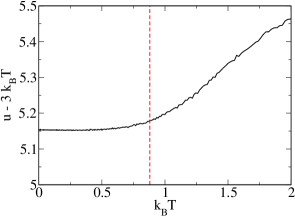
Figure 1: (Color online) Strictly anharmonic portion of the total average energy (kinetic and potential) per particle $u-3k_{B}T$ of the system in term of the thermostat temperature $T$. This is obtained by averaging over 10 cooling simulations of supercooled Z2 Dzugutov systems using $\tau_{10}=400$. $3k_{B}T$ has been subtracted from the energy to help identify the glass transition. The glass transition temperature $k_{B}T_{g}\sim 0.88$ is estimated by finding the temperature at which the function slope changes most rapidly. The vertical dashed line is located at $T=T_{g}$. The energy scale is normalized through our choice of potential parameters (see Sec. III).

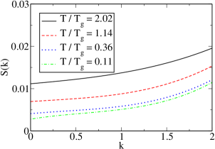
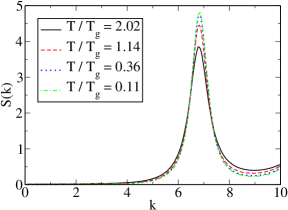
Figure 2: (Color online) Structure factors $S(k)$ for Z2 Dzugutov systems supercooled using $\tau_{10}=500$ for various temperatures. The curves have been averaged over 10 realizations. 2 Cubic fits of the small-wavenumber ($k<2$) structure factors. The type of fits and their cutoff are chosen such that they accurately reproduce the features of the structure factors, in particular the positive linear dependence near $k=0$. 2 Larger-wavenumber structure factors.

To calculate the volume integral of the direct correlation function $c(r)$, we need to find the limit of $S(k)$ for $k\rightarrow 0$, and then substitute it in Eq. (2). Since $S(k=0)$ cannot be calculated directly in a finite simulation box of side length $L$ because the smallest possible wavenumber accessible is $2\pi/L$, an extrapolation from the available data to zero wavenumber must be used. Figure 2 shows the small-wavelength behavior of $S(k)$ for Z2 Dzugutov model at different temperatures. It is clear that $S(k)$ is nearly linear in $k$ for $k\lesssim 1$, leading to a very good fit to a linear function. This linear behavior of $S(k)$ for small $k>0$ implies that the real-space total correlation function $h(r)$ decays, for large but finite $r$, as a power law $-1/r^{4}$ or, equivalently, the direct correlation function decays as $c(r)\sim-1/r^{2}$. The numerical value of $S(k=0)$ only changes by up to 5% between the cubic fit for $k<2$ shown in Fig. 2 and a linear fit for $k<1$. Since the linear fit is less susceptible to overfitting and complex behavior for $1<k<2$, we elect to use this linear fit to extrapolate the value of $S(k=0)$ for these systems.

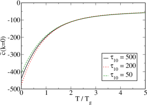
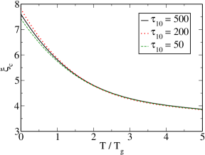
Figure 3: (Color online) Growing length scales for Z2 Dzugutov systems generated using various cooling schedules. For each cooling schedule, the results have been averaged over 10 realizations and fitted to the sum of an exponential and a linear function to smooth out the numerical noise. 3 Limit of $\widetilde{c}(k)$ for $k\rightarrow 0$, calculated using linear fits of $S(k)$. 3 The static length scale $\xi_{c}$, defined by relation (47), associated with these systems. Note that the nearest neighbor distance between particles at $T=0$ is $1.0539$.

From the Fourier transform of the direct correlation function $\widetilde{c}(k)$, which has units of volume, we define the following length scale:

$$\xi_{c}\equiv\left[-\widetilde{c}(0)\right]^{1/d},$$ (47)

where $d$ is the Euclidean dimension. From Fig. 3, there is a striking evidence that $\widetilde{c}(k=0)$ grows to a large negative value in the supercooled regime, leading to a doubling in the value of the length scale $\xi_{c}$.

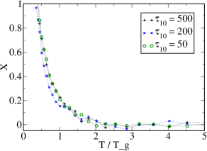
Figure 4: (Color online) Nonequilibrium index $X$ for Z2 Dzugutov systems supercooled using various cooling schedules defined in Eq. (49).

In the case of a single-component system at equilibrium, the compressibility relation links its isothermal compressibility $\kappa_{T}=-\frac{1}{V}\left.\frac{\partial V}{\partial p}\right|_{T}$ to its structure factor as follows:

$$\rho\kappa_{T}k_{B}T=S(0).$$ (48)

However, supercooled liquids and glasses are not equilibrium states and consequently Eq. (48) tends not to be satisfied. Following Ref. Ho12, , we use the deviation from Eq. (48) to measure a nonequilibrium index $X$:

$$X\equiv\frac{S(0)}{\rho\kappa_{T}k_{B}T}-1.$$ (49)

The isothermal compressibility $\kappa_{T}$ is computed by the following finite difference formula:

$$\kappa_{T}\simeq-\frac{\Delta V}{V}\frac{1}{\Delta P},$$ (50)

where $\Delta V$ is the change in volume of the simulation box and $\Delta P$ is the resulting change in pressure of the system after it is allowed to relax at constant temperature. The pressure is calculated using the virial relation. It bears mentioning that since the system is not at equilibrium, it is not in a steady state even before the change in volume. To minimize the impact of the uncompressed system relaxation, both the uncompressed and compressed systems are allowed to relax for the same amount of time before measuring their pressures.

In the case of the Z2 Dzugutov system, we use a change of volume $\Delta V/V=0.3\%$ and the pressure is sampled from $t=5$ to $t=10$, where $t=0$ denotes the time at which the system is compressed. As can be seen in Fig. 4, $X$ is zerofootnote:zeroX for $T/T_{g}>2$, with only slight deviations due to noise and numerical inaccuracies. However, as the temperature is lowered to values approaching the glass transition, $X$ increases up to a value of $\sim 0.2$ at $T/T_{g}=1$. For $T<T_{g}$, the inability of the system to relax in a time of the order of the cooling schedule time per decade $\tau_{10}$ results in nearly constant values of $\kappa_{T}$ and $S(0)$ which leads to the asymptotic behavior of $X$ as $T\rightarrow 0$.

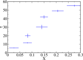
Figure 5: (Color online) Timescale $\tau$ of the early relaxation process of the system versus the nonequilibrium index $X$. Both quantities have been averaged over 10 configurations. The circle are centered on the averages of $X$ and $\tau$, while the horizontal and vertical lines represent their respective uncertainties, with their half-length set equal to the average standard deviations. The initial configurations which are allowed to relax at constant temperature are generated from the liquid phase through a cooling schedule employing $\tau_{10}=50$. Each datum represents a single temperature. Observe that $\tau$ and $X$ are positively correlated. Therefore, since $X$ is a monotonically decreasing function of the temperature $T$ (see Fig 4), $\tau$ also increases with decreasing $T$. The values of $T/T_{g}$ associated with each datum are, in order of smallest to largest $\tau$ are as follows: 1.80, 1.61, 1.43, 1.28, 1.14, 1.01, and 0.90.

Is the growing nonequilibrium index $X$, a purely static quantity, correlated with the growing relaxation times as the temperature decreases during the supercooling process? Figure 5 shows a positive correlation between $X$ and $\tau$, where $\tau$ is the timescale associated with the early relaxation process, extracted from an exponential fit function $\sim e^{-t/\tau}$ of the system total energy. To observe this process, we start with configurations that have been supercooled to a given temperature following a specific cooling schedule. These configurations are then allowed to evolve at constant temperature. It can be clearly seen that $X$ and $\tau$ are strongly and positively correlated.

IV.2 Kob-Andersen $A_{65}B_{35}$ Two-Component Glass

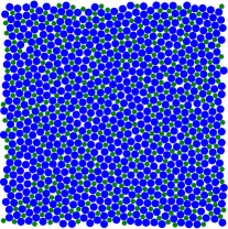
Figure 6: (Color online) Example of a decorated Kob-Andersen glass configuration (a small subregion of the configuration only). The larger disks represent the $A$ particles, while the smaller disks represent B particles. The radii of the disks are chosen such that the two closest $A$ particles of the whole configuration are in contact and the closest $A$–$B$ pair of particles are in contact. The configuration shown has been generated using $\tau_{10}=100$, and is at a temperature of $T/T_{g}=6.7\times 10^{-5}$. The particle radii are $R_{A}=0.513720$ and $R_{B}=0.329883$ ($R_{A}/R_{B}=1.55728$).

To calculate the spectral density $\widetilde{\chi}(k)$, we decorate the systems by circumscribing disks of radius $R_{A}$ and $R_{B}$ centered around the point particles of species $A$ and $B$, respectively. Since our derivation in Sec. II.2 requires the disks to be nonoverlapping, we chose the largest possible radii that satisfy this condition. In the case of a Kob-Andersen glass, $A$ particles are often located next to one another, while $B$ particles can be further apart. This leads to our decision to use the distances between the closest $A$–$A$ and $A$–$B$ pairs of particles to define the particle radii. Figure 6 shows part of a glass configuration decorated using this procedure.

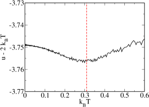
Figure 7: (Color online) Strictly anharmonic portion of the total average energy (kinetic and potential) per particle $u-2k_{B}T$ of the system in terms of the thermostat temperature $T$. This is obtained by averaging 10 cooling simulations of supercooled Kob-Andersen systems using $\tau_{10}=400$. $2k_{B}T$ has been subtracted from the energy to help identify the glass transition. The glass transition temperature $T_{g}\sim 0.31$ is estimated by finding the temperature at which the function slope changes the most rapidly. The vertical dashed line is located at $T=T_{g}$. The energy scale is normalized through our choice of potential parameters (see Sec. III).

In an identical fashion to the Z2 Dzugutov system, we use the change in slope of the total energy in terms of the temperature to estimate the glass transition temperature $T_{g}$ for the Kob-Andersen system. Since the Kob-Andersen system that we analyze is two-dimensional, its harmonic contribution to the energy is $2k_{B}T$, which we subtract from the total average energy per particle $u$ to detect any change of slope. The result obtained from Fig. 7 is $T_{g}\sim 0.31$, which is reasonably close to the previously-reported value of $T_{g}=0.33$. Brüning et al. (2009)

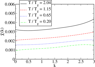
Figure 8: (Color online) Spectral density $\widetilde{\chi}(k)$ versus wavenumber $k$ for Kob-Andersen $A_{65}B_{35}$ systems supercooled using $\tau_{10}=400$. The curves have been averaged over 10 realizations and fitted using fourth degree polynomials. The type of fits have been chosen for their ability to reproduce accurately the features of the structure factors for the range presented ($0<k<3$). The disk radii for the decorations are calculated independently for each configuration.

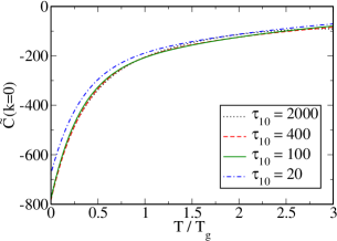
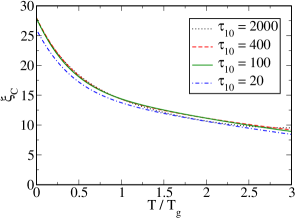
Figure 9: (Color online) Growing length scales for two-dimensional Kob-Andersen systems. For each cooling schedule, the results have been averaged over 10 realizations and fitted to the sum of an exponential and a quadratic functions to smooth out the numerical noise. 9 Limit of $\widetilde{C}(k)$ for $k\rightarrow 0$, calculated using the linear fits of $\widetilde{\chi}(k)$. 9 The static length scale $\xi_{C}$, defined by relation (51), associated with these systems.

As in the case of Z2 Dzugutov systems, the spectral densities $\widetilde{\chi}(k)$ for Kob-Andersen liquids, supercooled liquids, and glasses have nearly linear behavior for $k\lesssim 1$. It is thus possible to prescribe a linear fit to extrapolate the values of $\widetilde{\chi}(k=0)$, which is required to calculate $\widetilde{C}(k=0)$ using Eq. (24). We again define a length scale based on the $\widetilde{C}(k=0)$:

$$\xi_{C}\equiv\left[-\widetilde{C}(0)\right]^{1/d},$$ (51)

where $d$ is the Euclidean dimension. Figure 9 shows the large change in value of $\widetilde{C}(k=0)$ as the Kob-Andersen liquids are supercooled, leading to the length scale $\xi_{C}$ to increase by a factor larger than 5 between the fluid states and the zero-temperature glassy states.

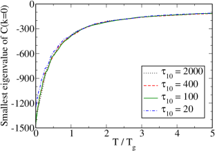
Figure 10: (Color online) Smallest eigenvalue of $\lim_{k\rightarrow 0}\mathbf{C}(k)$, calculated using a linear fit of the matrix structure factor $\mathbf{S}(k)$. While the qualitative behavior of this eigenvalue can be compared to $\widetilde{C}(k=0)$ (see Fig. 9), their quantitative values cannot directly be compared because they have different units: $\widetilde{C}(k)$ has units of volume, while $\widetilde{\mathbf{C}}(k)$ is dimensionless.

As mentioned in Sec. II.2.2, there is a second generalization of the direct correlation function which does not require any a priori knowledge or about the particle shapes. Instead, one can use the matrix direct correlation function $\mathbf{C}(r)$ and its Fourier transform $\widetilde{\mathbf{C}}(k)$. As can be observed in Fig. 10, the qualitative behavior of the smallest eigenvalue of $\widetilde{\mathbf{C}}(k)$ in the $k\rightarrow 0$ limit is strikingly close to the behavior of $\widetilde{C}(k)$ in the same limit. This indicates that our decoration choice is appropriate for detecting long-range density fluctuations in Kob-Andersen glasses and supercooled liquids.

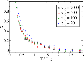
Figure 11: (Color online) Nonequilibrium index $X$ for Kob-Andersen systems supercooled using various cooling schedules defined in Eq. (54).

Since the compressibility relation (48) applies only to single-component systems, we must generalize the nonequilibrium index $X$ for mixtures. The compressibility relation for multicomponent systems at equilibrium, is given by:Kirkwood1951

$$\kappa_{T}k_{B}T=\frac{|\mathbf{B}|}{\sum_{\alpha=1}^{M}\sum_{\beta=1}^{M}|\mathbf{B}|_{\alpha\beta}},$$ (52)

where the components $B_{\alpha\beta}$ of the matrix $\mathbf{B}$ are

$$B_{\alpha\beta}=\frac{\sqrt{N_{\alpha}N_{\beta}}}{V}\lim_{k\rightarrow 0}S_{\alpha\beta}(k),$$ (53)

$|\mathbf{B}|$ is the determinant of $\mathbf{B}$, and $|\mathbf{B}|_{\alpha\beta}$ is the $\alpha\beta$ minor of $\mathbf{B}$. The nonequilibrium index $X$ for multicomponent systems can now be defined by using the mismatch between the left and right sides of Eq. (52), that is,

$$X\equiv\frac{|\mathbf{B}|}{\kappa_{T}k_{B}T\sum_{\alpha=1}^{M}\sum_{\beta=1}^{M}|\mathbf{B}|_{\alpha\beta}}-1.$$ (54)

As for single-component systems, the isothermal compressibility for this multicomponent system is obtained by computing the virial pressure response to an incremental change in volume using Eq. (50).

For the Kob-Andersen system, we use a change of volume $\Delta V/V=0.2\%$ and the pressure is sampled from $t=20$ to $t=40$, where $t=0$ denotes the time at which the quenching is halted and the system is compressed. As can be seen in Fig. 11, $X$ is zerofootnote:zeroX for $T>2T_{g}$. Similarly to the phenomenon observed in the case of the Z2 Dzugutov system (see Fig. 4), $X$ increases up to a value of a value of $\sim 0.15$ at $T=T_{g}$. The asymptotic behavior of $X$ for $T<T_{g}$ is again the consequence of the system inability to relax in a time comparable to the cooling schedule time per decade $\tau_{10}$.

V Conclusions and Discussion

We have demonstrated here that the static structural length scales $\xi_{c}$ and $\xi_{C}$ are able to distinguish subtle structural differences between glassy and liquid states, which extends the analogous results for metastable hard spheres Ho12 to atomic thermal systems. Since these length scales are based on the volume integral of the direct correlation function $c(r)$ and its generalization $C(r)$, respectively, their growth as a liquid is cooled past its glass transition is a sign of the presence of long-range correlations in the glassy state that are not present in liquids. Additionally, the continuing increase of $\xi_{c}$ and $\xi_{C}$ past the glass transition indicates that, while particles primarily undergo sequences of local rearrangements, the glass may still exhibit order on a significantly larger length scale as the system continues to cool. Our results using two-dimensional Kob-Andersen binary mixtures and three-dimensional Z2 Dzugutov single-component systems, as well as the previous results for MRJ packings as evidence, we postulate that these length scales are relevant in various glasses. This includes not only atomic systems possessing pair potentials with steep repulsions and short-range attractions, but network glasses as well. For example, in a recent computational study,Henja2012 which is supported by recent experimental results,Long et al. (March 11th-15th, 2012) it was shown that realistic models of amorphous silicon can be constructed to be nearly hyperuniform, which implies that such glassy tetrahedrally-coordinated networks are characterized by a large static length scale $\xi_{c}$ We also have shown that the nonequilibrium index $X$ is positively correlated with a characteristic relaxation time scale, since they both increase as a system is supercooled.

An interesting issue concerns the explication of the underlying geometrical reasons for the negative algebraic tail in the pair correlation function,Donev et al. (2005a) which also has been observed in hard-sphere systems.Ho12 (The former is exhibited for large but bounded pair distances, while the latter is valid asymptotically as $r\rightarrow\infty$.) The local geometric diversity of particle arrangements in an amorphous solid medium inevitably creates short-range density fluctuations. In particular, this is true for the nearly hyperuniform cases examined in this study. Without being too specific, one can formally divide a “jammed” particle configuration into two equal subsets containing particles experiencing either lower or higher local densities than the overall system average. The fact that the pair correlation functions display negative algebraic tails with increasing separation $r$ has basic implications for the relative spatial distributions of these low and high local density particles. In particular, it indicates that large numbers of either particle type cannot fit together to form arbitrarily large clusters that dominantly exclude the other particle types. Instead, their spatial patterns evidently involve interpenetrating percolating networks in three dimensions and highly non-convex clusters in two dimensions. The detailed statistical geometric description of these patterns and why they generate algebraic pair correlation function tails constitutes an important area for future investigation.

The quantity $X$ introduced earlier in Eq. (49) as a measure of deviation from thermal equilibrium can be usefully interpreted in terms of system occupancy on the many-body potential energy landscape.Stillinger1998 Specifically, this focuses on the comparative behaviors of isothermal compressibility at high-temperature thermal equilibrium in the liquid phase as opposed to the measured isothermal compressibility in the non-equilibrium glass phase in the $T\rightarrow 0$ limit. In the former case, an incremental pressure change and accompanying volume change will include shifts in occupancy probabilities for the separate basins that tile the landscape; these shifts involve interbasin local particle rearrangements that act to enhance the volume change induced by the pressure perturbation. In contrast, at very low temperatures, the system is trapped in its initial basin; intrabasin vibrational motions have insufficient amplitude to allow the system to take advantage of the previous kinds of local particle rearrangements. The resulting absence of enhanced volume change due to those interbasin transitions reduces isothermal compressibility, causing $X$ to increase above zero.

References

- Chaikin and Lubensky (1995) P. M. Chaikin and T. C. Lubensky, Principles of Condensed Matter Physics (Cambridge, 1995).
- Berthier et al. (2007) L. Berthier, G. Biroli, J.-P. Bouchaud, J. W. Kob, K. Miyazaki, and D. R. Reichman, J. Phys. Chem. 126, 184503 (2007).
- Karmakar et al. (2009) S. Karmakar, C. Dasgupta, and S. Sastry, PNAS US 106, 3675 (2009).
- Chandler and Garrahan (2010) D. Chandler and J. P. Garrahan, Ann. Rev. Phys. Chem. 61, 191 (2010).
- Lubchenko and Wolynes (2006) V. Lubchenko and P. G. Wolynes, Ann. Rev. Phys. Chem. 58, 235 (2006).
- Hocky et al. (2012) G. M. Hocky, T. E. Markland, and D. R. Reichman (2012), eprint arXiv:1201.2888.
- (7) A. B. Hopkins, F. H. Stillinger, and S. Torquato, Phys. Rev. E, 82, 021505 (2012).
- Torquato et al. (2000) S. Torquato, T. M. Truskett, and P. G. Debenedetti, Phys. Rev. Lett. 84, 2064 (2000).
- Torquato and Stillinger (2010) S. Torquato and F. H. Stillinger, Rev. Mod. Phys. 82, 2633 (2010).
- Torquato and Stillinger (2007) S. Torquato and F. H. Stillinger, J. App. Phys. 102, 093511 (2007); ibid 103, 129902 (2008).
- Torquato and Stillinger (2003) S. Torquato and F. H. Stillinger, Phys. Rev. E 68, 041113 (2003).
- Hansen and McDonald (2006) J. P. Hansen and I. R. McDonald, Theory of Simple Liquids, 3rd ed. (Academic, 2006).
- Donev et al. (2005a) A. Donev, F. H. Stillinger, and S. Torquato, Phys. Rev. Lett. 95, 090604 (2005a).
- Doye et al. (2003) J. P. K. Doye, D. J. Wales, F. H. M. Zetterling, and M. Dzugutov, J. Chem. Phys. 118, 2792 (2003).
- Kob and Andersen (1994) W. Kob and H. C. Andersen, Phys. Rev. Lett. 73, 1376 (1994).
- (16) M. D. Rintoul and S. Torquato, Phys. Rev. Lett. 77, 4198 (1996); M. D. Rintoul and S. Torquato, J. Chem. Phys. 105, 9258 (1996).
- (17) K. S. Schweizer, J. Chem. Phys. 127, 16506 (2007).
- Zachary et al. (2011) C. E. Zachary, Y. Jiao, and S. Torquato, Phys. Rev. Lett. 106, 178001 (2011); C. E. Zachary, Y. Jiao, and S. Torquato. Phys. Rev. E, 83, 051308 (2011).
- end (c) The hyperuniformity of maximally random jammed packings has been extended to apply to polydisperse spheres and nonspherical objects in terms of the spectral density .Zachary et al. (2011)
- (20) S. Torquato and G. Stell, J. Chem. Phys. 82, 980 (1985).
- (21) S. Torquato, Random Heterogeneous Materials (Springer, 2002).
- Baxter (1970) R. J. Baxter, J. Chem. Phys. 52, 4559 (1970).
- (23) Using expression (41) to write for a single configuration, we can express as the product of a non-zero vector times its Hermitian transpose, the rank of which (equal to the number of non-zero eigenvalues) is 1. Taking an ensemble average of Eq. (41) breaks this symmetry, since the sum of vectors multiplied by their transpose has a rank of if the vectors are linearly independent.
- (24) W. G. Hoover, Phys. Rev. A 31, 1695 (1985).
- (25) B. Widom, J. Chem. Phys. 52, 3888 (1970).
- (26) Note that we found a very small systematic error due to a combination of the following factors: the thermostat, relaxation during the compressibility computation, and the finite difference method. To correct for this systematic error, we added to the computed value of a constant such as to ensure that for the high-temperature liquid phase, for which the compressibility relations (48) and (52) are satisfied. This constant is equal to for the Z2 Dzugutov potential, and for the Kob-Andersen potential.
- Brüning et al. (2009) R. Brüning, D. A. St-Onge, S. Patterson, and W. Kob, J. Phys.: Conden. Matter 21, 035117 (2009).
- (28) J. G. Kirkwood and F. P. Buff, J. Chem. Phys. 19, 774 (1951).
- (29) M. Henja, P. J. Steinhardt, and S. Torquato, submitted for publication.
- Long et al. (March 11th-15th, 2012) G. Long, R. Xie, S. Weigand, S. Moss, S. Roorda, S. Torquato, and P. Steinhardt, Proceedings of the Minerals, Metals and Materials Society (March 11th-15th, 2012), Orlando, FL (to be published).
- (31) F. H. Stillinger, P. G. Debenedetti, and S. Sastry, J. Chem. Phys. 109, 3983 (1998).