Hot accretion flow in black hole binaries: a link connecting X-rays to the infrared

Abstract

Multiwavelength observations of Galactic black hole transients have opened a new path to understanding the physics of the innermost parts of the accretion flows. While the processes giving rise to their X-ray continuum have been studied extensively, the emission in the optical and infrared (OIR) energy bands was less investigated and remains poorly understood. The standard accretion disc, which may contribute to the flux at these wavelengths, is not capable of explaining a number of observables: the infrared excesses, fast OIR variability and a complicated correlation with the X-rays. It was suggested that these energy bands are dominated by the jet emission, however, this scenario does not work in a number of cases. We propose here an alternative, namely that most of the OIR emission is produced by the extended hot accretion flow. In this scenario, the OIR bands are dominated by the synchrotron radiation from the non-thermal electrons. An additional contribution is expected from the outer irradiated part of the accretion disc heated by the X-rays. We discuss properties of the model and compare them to the data. We show that the hot-flow scenario is consistent with many of the observed spectral data, at the same time naturally explaining X-ray timing properties, fast OIR variability and its correlation with the X-rays.

1 Introduction

Although the black hole X-ray binaries (BHBs) have been intensively studied for over four decades, many problems remain unsolved. Among the most debated topics are the physics of state transitions, the interplay between the cold accretion disc and the hot medium, the role of the jet, the source of rapid variability, radiative processes shaping the broadband spectrum and, specifically, the nature of various components contributing to its different parts. When addressing the latter problem, three distinct components are usually considered: the standard (or irradiated) cool accretion disc, the hot inner flow (or corona) and the jet. Their relative contribution depends on the spectral energy range and varies with time and can be assessed by performing (quasi-) simultaneous multiwavelength observations.

Over the past decade, numerous multiwavelength campaigns have resulted in a significant progress in the field. Broadband radio to X-ray spectral energy distributions (SEDs) for many black holes (BH) low-mass X-ray binaries (LMXBs) were constructed (e.g. Hynes et al., 2000; McClintock et al., 2001; Chaty et al., 2003; Cadolle Bel et al., 2007, 2011; Durant et al., 2009). In addition to the spectral information, data on the fast variability are now available in the X-rays as well as at lower energies. The light curves in the optical/infrared (OIR) and ultraviolet (UV) bands are significantly correlated with the X-rays (Kanbach et al., 2001; Hynes et al., 2003, 2006, 2009b; Durant et al., 2008, 2011; Gandhi et al., 2010) showing a complex shape of the cross-correlation function (CCF). It provides an important information on the interrelation between various components and gives clues to their physical origin.

The radio emission in BHBs is likely dominated by the jet as supported by the observed linear polarization at a 1–3 per cent level in the hard state (Corbel et al., 2000) and up to ten per cent in spatially resolved components during the transient events (Fender et al., 1999; Hannikainen et al., 2000). In addition, a relatively high luminosity, requiring the size exceeding the typical binary separation (Fender, 2006), as well as the detection of superluminal motion (Mirabel & Rodríguez, 1994) lean towards this interpretation. The power-law-like radio spectrum is often attributed to synchrotron emission of an inhomogeneous source in analogy with the extragalactic jets (Blandford & Königl, 1979). In blazars, the jet is also responsible for the X-ray and $\gamma$-ray production (Königl, 1981; Dermer & Schlickeiser, 1993; Sikora, Begelman & Rees, 1994; Stern & Poutanen, 2006). On the contrary, the jets in BHBs are unlikely to be responsible for bulk of the X-ray photons (for comprehensive discussion see Poutanen & Zdziarski, 2003; Zdziarski et al., 2003). Further, the medium producing the X-ray radiation can neither form the base of the jet (Malzac, Belmont & Fabian, 2009), nor be a jet-dominated accretion flow (Maccarone, 2005).

The spectra of hard-state BHBs constitute a power-law in the X-ray band with a stable spectral slope and ubiquitous sharp cut-off at $\sim$100 keV (Gierlinski et al., 1997; Zdziarski et al., 1998; Ibragimov et al., 2005). It is broadly accepted to be produced by thermal Comptonization (e.g. Poutanen, 1998; Zdziarski & Gierliński, 2004). Additionally, a Compton reflection feature originating from cool opaque matter (likely the cool accretion disc) is often detected. Its strength is correlated with the X-ray slope (Zdziarski, Lubinski & Smith 1999; Zdziarski et al. 2003), with the width of the iron line as well as with the quasi-periodic oscillation (QPO) frequency (Gilfanov, Churazov & Revnivtsev, 1999; Revnivtsev, Gilfanov & Churazov, 2001; Gilfanov, 2010). These observations support a view that the X-rays are produced in the very vicinity of the BH, in a hot flow surrounded by the cold disc. In this scenario, variations in the mass accretion rate are correlated with the cool disc truncation radius (Esin, McClintock & Narayan, 1997; Poutanen, Krolik & Ryde, 1997), with the flux of soft seed photons that determines the spectral slope and with the reflection amplitude that scales with the solid angle at which the cold disc is seen from the hot flow. Correlations with the QPO frequency are also naturally explained if the oscillations are produced in the innermost part of the accretion flow by Lense–Thirring precession (Ingram & Done, 2011). Such a scenario would favour models where seed photons for Comptonization are provided by the standard Shakura & Sunyaev (1973) accretion disc. However, the hot flow itself also produces synchrotron radiation that can contribute or even dominate the seed photon flux to the Comptonizing medium (Ghisellini, Haardt & Svensson 1998; Wardziński & Zdziarski 2000, 2001; Malzac & Belmont 2009; Poutanen & Vurm 2009; Sobolewska et al. 2011; Veledina, Vurm & Poutanen 2011b).

Discovery of the high-energy (MeV) tails in the hard-state accreting BHBs (McConnell et al. 1994, 2002; Ling et al. 1997; Droulans et al. 2010; Jourdain, Roques, & Malzac 2012b) suggests the presence of non-thermal particles in these systems. Such particles may be produced in a hot inner flow or a jet. Their association with the jet, however, is inconsistent with detections of even more prominent high-energy non-thermal tails in the soft state of BHBs (Grove et al., 1998; Gierliński et al., 1999; Zdziarski et al., 2001; McConnell et al., 2002; Gierliński & Done, 2003), when the jet is quenched (Fender, Belloni & Gallo, 2004). In this state the inner flow is likely to be replaced by a corona, which remains here the only alternative. In the hard state, the entire X/$\gamma$-ray spectra can be produced by hybrid (thermal plus non-thermal) electrons via synchrotron self-Compton (SSC) mechanism (Malzac & Belmont, 2009; Poutanen & Vurm, 2009). The thermal part of the particle distribution is responsible for the power-law-like Comptonization continuum with the sharp cut-off, while the non-thermal particles both produce seed synchrotron photons for Comptonization and contribute to the MeV energies via inverse Compton process. Transition to the soft state can then be associated with the rising role of the disc as a source of seed photons, which increases Compton cooling and causes changes in the electron distribution from mostly thermal to nearly non-thermal (Poutanen & Coppi, 1998; Poutanen & Vurm, 2009; Veledina et al., 2011b). The SSC mechanism was also shown to be consistent with the peculiar optical variability, which in a number of BHBs is partially anticorrelated with the X-ray emission (Kanbach et al., 2001; Durant et al., 2008; Gandhi et al., 2008). Namely, the increasing mass accretion rate results in a higher X-ray and a lower synchrotron OIR emission, because of an increasing role of synchrotron self-absorption within the source (Veledina, Poutanen & Vurm, 2011a).

The OIR spectra of LMXBs often show an excess above the standard accretion disc (e.g., Hynes et al. 2000, 2002; Gelino, Gelino & Harrison 2010). In some cases the spectrum can be described by a power-law of index close to zero (i.e. $F_{\nu}\propto\nu^{0}$). Such data were previously explained by additional contribution from the irradiated disc (Gierliński, Done & Page, 2009), dust heated by the secondary star (Muno & Mauerhan, 2006) or the jet (Hynes et al., 2002; Gallo et al., 2007). We show that they also can be explained by the synchrotron radiation from the non-thermal particles in the hot flow. However, in some cases the OIR fluxes are higher than expected from any candidate alone (Chaty et al., 2003; Gandhi et al., 2010), suggesting contribution of at least two components simultaneously. This can be a reason for the complex shape of the optical/X-ray CCF (Veledina et al., 2011a).

The general shape of the time-averaged X/$\gamma$-ray spectrum of BHB can be well explained in terms of a one-zone hybrid Comptonization model. However, the short-term spectral variability, reflected in hard X-ray time-lags (Miyamoto & Kitamoto, 1989; Nowak et al., 1999a), and asymmetries of the CCF between hard and soft X-ray energy bands (Priedhorsky et al. 1979; Nolan et al. 1981; Maccarone, Coppi & Poutanen 2000) suggest that a number of regions simultaneously contribute to the total spectrum. The observed logarithmic dependence of the time-lags on photon energy can be phenomenologically explained by spectral pivoting (Poutanen & Fabian, 1999). Theoretical model capable of explaining the observed timing properties was proposed by Kotov, Churazov & Gilfanov (2001) and further developed in Arévalo & Uttley (2006). It assumes that the X-ray spectrum is produced in the hot flow/corona, present in a range of radii, by Comptonization of the disc photons. The power-law slope of the locally emitted spectrum depends on the distance from the BH: the hardest spectra are produced in the innermost region due to the lack of photons from the cold disc. The main source of the short-term variability in BHs is believed to be fluctuations in the mass accretion rate, propagating through the hot accretion flow (Lyubarskii, 1997). The hard time-lags thus naturally appear from the perturbations propagating from the larger distances to the vicinity of the BH. The model of Kotov et al. (2001) considers thermal Comptonization of the disc photons, but as we show below the results hold in the framework of hybrid Comptonization, with the synchrotron mechanism as the major seed photon supplier.

It is clear that the complete description of the timing and spectral properties of BHBs requires a multizone model. In this paper we construct such a model for the extended hot accretion flow. This model is somewhat analogous to the inhomogeneous synchrotron models developed for extragalactic jets (Marscher, 1977; Blandford & Königl, 1979). The difference is that in our model the emission originates from an inflow, not an outflow. The advantage of the hot-flow model is that the energy input can be estimated from the available gravitational energy transferred to particles via some mechanism, while in the jet scenario the energy release is an arbitrary function.

Similarly to the previously studied one-zone models (Malzac & Belmont, 2009; Poutanen & Vurm, 2009; Veledina et al., 2011b), we assume that gravitational energy is dissipated in the flow and injected in the form of electrons having a power-law distribution (while the steady-state electron distribution is mostly thermal). We compute the steady-state particle and photon distributions self-consistently by solving corresponding kinetic equations. Our aim is to understand the broadband spectral properties of such a flow and compare them to the BHB data.

Figure 1: Schematic picture of the accretion flow inner regions. Red outer component represents the multi-color cold accretion disc, truncated at 300 Schwarzschild radii ($R_{\rm S}$). The inner parts are occupied by a geometrically thick hot accretion flow. In our numerical model, we split the inner hot flow into four zones with outer radii $10R_{\rm S}$ (violet), $30R_{\rm S}$ (blue), $100R_{\rm S}$ (green) and $300R_{\rm S}$ (yellow).

In Section 2, we give constraints on the size of the hot accretion flow that can be derived from the observed level of the OIR emission. We first construct an analytical model for the hot flow assuming power-law radial dependences of the main parameters. We then proceed to the numerical model where the electron distributions and the emitted spectra are computed self-consistently. In Section 3, we present the results of simulations for the model corresponding to the hard state of BHBs. We show that the multizone hot disc model produces flat OIR spectra resulting from synchrotron emission of non-thermal electrons at different radii. We then model the state transitions by decreasing the truncation radius of the hot flow. In Section 4, we provide a detailed analysis of the observational data and compare them to our model and to the jet scenario. We summarize our finding in Section 5.

2 Analytical model

2.1 Geometry

Many observational properties suggest that the standard disc in the hard state is truncated far away from the central object (for detailed description and challenges to the truncated disc scenario, see review by Done et al., 2007). The inner part is probably occupied by some type of geometrically thick, optically thin, hot accretion flow, which is responsible for the X-ray Comptonization continuum, but also contributes to the longer wavelengths.

One can roughly estimate the minimum size of the source that is required to produce the observed OIR luminosity. Let us first assume that OIR emission is produced by synchrotron radiation from thermal particles (as for example was discussed earlier by Fabian et al. 1982). The typical temperature of the electron gas determined from the Comptonization cut-off is $kT_{\rm e}$$\sim$100 keV and the typical IR luminosity at $1$ eV can reach $\nu L_{\nu,\rm 1\ eV}=10^{36}$ erg s^-1. Thus, we get the minimum size from the Rayleigh-Jeans formula

$$R=\left(\frac{\nu L_{\nu}}{8\pi^{2}\nu(\nu/c)^{2}kT_{\rm e}}\right)^{1/2}\approx 2.3\times 10^{9}\ \mbox{cm}.$$ (1)

For a 10$\mbox{M}_{\odot}$ BH, assumed in all calculations hereafter, this corresponds to 750 $R_{\rm S}$ (here $R_{\rm S}=2GM/c^{2}$ is the Schwarzschild radius). However, many observed properties [e.g. iron line width, amplitude of Compton reflection, drop of the iron line equivalent width with the Fourier frequency, see Gilfanov (2010), as well as dependence of the X-ray time-lags on energy below $\sim$1 keV, Uttley et al. (2011)] suggest that the cold disc in the hard state is truncated at a smaller radius. Moreover, in order to produce sufficient amount of seed photons for Comptonization, an extremely high magnetic field is required in addition to the large source size (see Appendix B.1 and also, e.g., Di Matteo, Celotti & Fabian, 1999; Merloni, Di Matteo & Fabian, 2000). Thus, the thermal radiation of the hot flow is unlikely to be a good candidate to produce enough OIR photons (see also Wardziński & Zdziarski, 2000).

However, even a weak, energetically unimportant non-thermal tail, in addition to the mostly Maxwellian distribution, gives a significant rise to the synchrotron luminosity (e.g. Wardziński & Zdziarski, 2001). For example, a tail containing only one per cent of total particle energy increases it by a factor of $100$. Accurate calculations (see below) show that the source size of $R\approx(30-50)R_{\rm S}$, an order magnitude smaller than given by equation (1), would in principle be enough to radiate the observed OIR luminosity. Such a size is consistent with the above estimates of the truncation radius and with the typical size of the region of the gravitational energy release. It is worth noticing that a strong synchrotron emission from non-thermal particles makes it a good candidate for seed photons for Comptonization (Malzac & Belmont, 2009; Poutanen & Vurm, 2009), which implies that the SSC spectrum extends from the X-rays down to the OIR band with the low-energy turnover determined by the maximum extent of the hot flow.

2.2 Hard-state OIR spectra

Spectral properties of the hot flow in the OIR band can be understood from simple analytical considerations. Let us consider the flow with a constant height-to-radius ratio $H/R$, extending between radii $R_{\rm in}$ and $R_{\rm out}$ (see Fig. 1 for the geometry). In order to estimate the synchrotron luminosity and spectra, we assume that the electrons follow a power-law distribution in Lorentz factor $n_{\rm e}(\gamma)\equiv dn_{\rm e}/d\gamma=n_{0}\gamma^{-p}$, starting from $\gamma_{\rm le}=1$ to infinity. Deviations from the power-law at low energies do not play any role, as the synchrotron emission produced by these electrons is self-absorbed. The Thomson optical depth across the disc is assumed to follow the power law $\tau(R)\propto R^{-\theta}$. For the constant $H/R$ this is equivalent to $n_{0}(R)\propto\tau/R\propto R^{-\theta-1}$. We further assume that the magnetic field depends on the distance from the BH as $B(R)\propto R^{-\beta}$.

Our analytical model of the hot flow is analogous to the non-uniform synchrotron source models, previously applied to the emission from extragalactic jets (Condon & Dressel, 1973; de Bruyn, 1976; Marscher, 1977; Blandford & Königl, 1979; Königl, 1981; Ghisellini, Maraschi & Treves, 1985). For the parameters considered here, most of the luminosity is produced in the inner part of the source, so that the OIR spectrum is composed of emission components coming from different radii and is not dominated by the radiation from the outer regions (these two cases are illustrated in figs 2a and 2b in Ghisellini et al. 1985).

A region of the disc at a given radius emits synchrotron radiation, which is self-absorbed below the turnover frequency $\nu_{\rm t}$. For power-law electrons, this frequency can be calculated as (Rybicki & Lightman, 1979; Wardziński & Zdziarski, 2001)

$$\nu_{\rm t}=3^{\frac{p+1}{p+4}}2^{-\frac{6}{p+4}}\pi^{\frac{1}{p+4}}\nu_{\rm L}^{\frac{p+2}{p+4}}\left[G_{1}(p)cRr_{\rm e}n_{0}\right]^{\frac{2}{p+4}},$$ (2)

where $\nu_{\rm L}=eB/(2\pi m_{\rm e}c)$ is the Larmor frequency, $G_{1}(p)\simeq 1$ is a combination of Euler’s Gamma functions (due to averaging over electron pitch angles), $r_{\rm e}$ is the classical electron radius. Substituting the constants, we get

$$\nu_{\rm t}\approx 3\times 10^{15}B_{6}^{\frac{p+2}{p+4}}\left(\sigma_{\rm T}n_{0}R\right)^{\frac{2}{p+4}}{\rm Hz},$$ (3)

where $Q=10^{x}Q_{x}$ in cgs units. The term in brackets can also be written as $\sigma_{\rm T}n_{0}R=\tau(\gamma_{\rm t})\gamma_{\rm t}^{p}$, with $\gamma_{\rm t}$ being the Lorentz factor of the electrons emitting at the turnover frequency and $\tau(\gamma_{\rm t})=\sigma_{\rm T}Rn_{\rm e}(\gamma_{\rm t})$ being the Thomson optical depth per unit Lorentz factor at $\gamma_{\rm t}$. In the later representation, the equation is also valid for hybrid electrons (e.g., Maxwellian with power-law tail), as long as the electrons emitting at the turnover frequency are in the power-law tail. The low-frequency cut-off for synchrotron spectrum from power-law electrons scales as

$$\nu_{\rm t}\propto R^{-[\beta(p+2)+2\theta]/(p+4)}.$$ (4)

Again, for hybrid electron distribution one should consider scaling with radius of the power-law tail (parameter $\theta$), which can be different from scaling of the total optical depth. As immediately follows from equation (3), the turnover frequency may fall to optical and even IR wavelengths for sufficiently low magnetic field and/or Thomson optical depth.

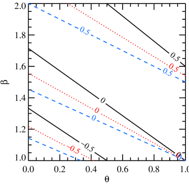
Figure 2: Contour plot of the constant index $\alpha_{\rm OIR}$ as a function of parameters $\beta$ and $\theta$ for three values of electron index $p$=$2$ (solid black), $3$ (dotted red) and $4$ (dashed blue).

The emission at the turnover frequency is optically thick, so the intensity is equal to the source function for the power-law electrons. For isotropic electrons the intensity is (averaged over pitch angles)

$$I_{\nu_{\rm t}}=\frac{m_{\rm e}G_{2}(p)}{2\sqrt{3}}\nu_{\rm L}^{-1/2}\nu_{\rm t}^{5/2},$$ (5)

where $G_{2}(p)\simeq 1$ (again, coming from the angle-averaging). At each wavelength, there is a contribution from the optically thick and optically thin emission from different radii. For simplicity, we assume that emission from each radius contributes only to its own turnover frequency, therefore the resulting spectrum of an inhomogeneous synchrotron source constitutes a power-law

$$\nu L_{\nu}=4\pi^{2}R^{2}\nu I_{\nu}\approx 2\times 10^{36}R_{8}^{2}\ B_{6}^{-1/2}\ \nu_{15}^{7/2}\;{\rm erg\,s}^{-1}.$$ (6)

Substituting the appropriate parameter scaling and using equation (4), we get the spectral index

$$\alpha_{\rm OIR}=\frac{5\theta+\beta(2p+3)-2p-8}{\beta(p+2)+2\theta},$$ (7)

where $\displaystyle L_{\nu}\propto\nu^{\alpha}$. In a wide range of parameters $\beta\in[1,2]$ and $\theta\in[0,1]$ the resulting spectral slope lies between $-0.5$ and $0.5$ (see Fig. 2).

3 Numerical model

The analytical model developed in Section 2.2 describes only the OIR synchrotron spectra and is valid for purely power-law electrons. Such distributions may result from various acceleration mechanisms e.g. shock acceleration or magnetic reconnection. In the limit of low optical depth and weak magnetic field the electrons are unable to cool and the shape of the distribution stays unchanged. These conditions might be satisfied in quiescent state, for which the analytical model can be applied. During the accretion outbursts, the matter density in the hot flow increases and the energy exchange and cooling processes become important; thus, the initial power-law distribution evolves. The most important mechanisms operating in the hot rarefied plasmas of the hot accretion flows are Compton scattering, synchrotron emission and absorption, Coulomb collisions, bremsstrahlung, and possibly photon-photon pair production and annihilation. At high energies, for a continuously operating acceleration, the steady state distribution remains a power-law-like, but softens because of cooling by Compton, synchrotron and bremsstrahlung. At lower energies, Coulomb collisions and synchrotron self-absorption efficiently thermalize particles, forming a Maxwellian distribution. The total particle distribution consists of a low-energy Maxwellian plus a high-energy tail. Such a distribution we call hybrid. The shape and energy content of the tail are fully determined by the balance between acceleration and cooling processes. It cannot be calculated analytically; therefore, we treat this problem numerically. The photon spectrum emitted by the hot flow is computed self-consistently with the particle distributions.

The time-scale of equilibration of electron and photon distributions for typical parameters of our model is smaller than the corresponding advection time in the hot flow (see Appendix A). Thus we can use an assumption that the electron and photon distributions are in a steady state. We obtain them by solving the relevant kinetic equations.

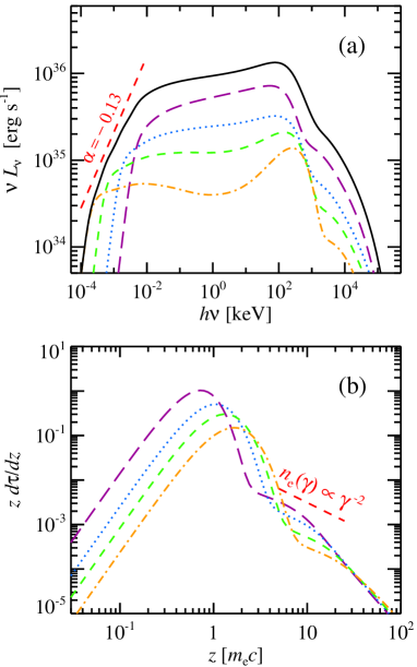
Figure 3: Photon spectra (upper panel) and electron distributions (lower panel) for the hard-state model with initial electron injection index $\Gamma_{\rm inj}=2.5$. Electron momenta $z=\sqrt{\gamma^{2}-1}$ are measured in units of $m_{\rm e}c$. Other parameters are listed in Table 1. The lines correspond to zone 1 (long-dashed), zone 2 (dotted), zone 3 (dashed) and zone 4 (dot-dashed). Sum of the components is shown with a solid line. The red short-dashed line shows the slopes from analytical approximation. For further details, see Section 3.2.

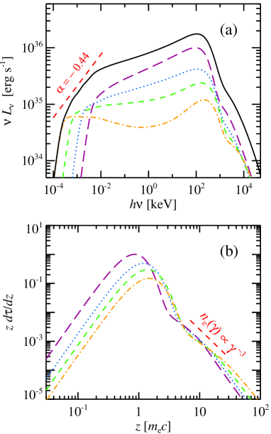
Figure 4: Same as Fig. 3, but for the electron injection index $\Gamma_{\rm inj}=3.0$. X-ray spectra are harder in this case, while the OIR spectrum is softer.

3.1 Model set up

We consider a geometrically thick optically thin inner accretion flow, which vertical extent is parametrized by the ratio $H/R=\rm const$. We assume that the hot flow corresponds to some type of radiatively inefficient accretion flow (see review in Kato, Fukue & Mineshige, 2008). In such flow, the radiative loss rate per unit area scales with radius as $\displaystyle Q_{\rm rad}\propto R^{-5/2}$, and the electron number density scales as $\displaystyle n_{\rm e}(R)\propto R^{-3/2}$. The Thomson optical depth along the vertical direction $\tau=\sigma_{\rm T}n_{\rm e}(R)H\propto{R}^{-1/2}$. The scaling of the magnetic field with radius is model-dependent (e.g., Shadmehri & Khajenabi, 2005; Meier, 2005; Akizuki & Fukue, 2006). Here we assume that the magnetic pressure and the radiation pressure are equal throughout the flow, from which we get $B\propto R^{-5/4}$. The latter scaling is the same as in the accretion flow model of Shadmehri & Khajenabi (2005). The hot flow extends from $3R_{\rm S}$ to the truncation radius $R_{\rm tr}$, where the cold disc with luminosity $L_{\rm disc}$ and colour temperature $T_{\rm col}$ starts.

The energy transfer to electrons is simulated as a power-law injection with slope $\Gamma_{\rm inj}$, extending between the Lorentz factors 1 and $10^{3}$. The model has seven parameters: (i) the total luminosity $L$, (ii) the index of the electron power-law injection spectrum $\Gamma_{\rm inj}$ (constant throughout the flow), (iii) the electron Thomson optical depth $\tau_{1}$ and (iv) the magnetic field $B_{1}$ in the innermost regions, (v-vi) indices of their power-law radial dependencies $\theta$ and $\beta$, and (vii) the hot-flow size $R_{\rm tr}$.

The energy given to electrons is redistributed between the particles (electrons and positrons) and photons in processes of synchrotron emission and self-absorption, Compton scattering, Coulomb collisions, pair production and annihilation and bremsstrahlung emission. The dominating cooling regime for a specific electron Lorentz factor depends on the luminosity, magnetic field and the optical depth (relevant scaling is given in Appendix A). In addition to the internally produced radiation, we also consider soft photons from the cold outer accretion disc in the form of the blackbody radiation injected homogeneously into the system. The kinetic equations for electrons and photons describing relevant radiative processes are solved using the code developed by Vurm & Poutanen (2009).

To compute the radiative transfer in the , we divide it into a number of separate regions/zones (Fig. 1). Each zone $i$ has size (in the radial direction) $\Delta R_{i}=R_{i+1}-R_{i}$ equal to its full height at the zone centre $2H_{i}=2R_{i,\rm c}(H/R)$ (where $R_{i,\rm c}=(R_{i}+R_{i+1})/2$ is the distance to the center of $i$th zone), implying

$$R_{i+1}=R_{i}\frac{1+H/R}{1-H/R}.$$ (8)

The net energy input into the $i$th zone equals to its luminosity:

$$L_{i}=2\pi\int\limits_{R_{i}}^{R_{i+1}}Q_{\rm rad}(R)RdR\propto\frac{1}{\sqrt{R_{i}}}-\frac{1}{\sqrt{R_{i+1}}}.$$ (9)

The characteristic Thomson optical depth of the $i$th zone is associated with that in the vertical extension

$$\tau_{i}=\sigma_{\rm T}n_{\rm e}(R_{i,\rm c})H_{i}.$$ (10)

Additional soft photons from the outer cold disc are described by the colour temperature $T_{\rm col}$ and the disc luminosity coming to the $i$th zone $(\Omega_{i}/4\pi)L_{\rm disc}$. Here the factor $\Omega_{i}$ accounts for the fact that only a part of the disc luminosity is entering the hot flow. It is fully determined by the cold disc/hot-flow geometry and in our case can be approximated as

$$\frac{\Omega_{i}}{4\pi}\approx\frac{1}{4}\left(\frac{R_{i+1}}{R_{\rm tr}}\right)^{3},$$ (11)

where $\pi(R_{i+1}/R_{\rm tr})^{2}$ is the solid angle of the $i$th zone as seen from the cold accretion disc, and another factor of $R_{i+1}/R_{\rm tr}$ accounts for anisotropy of the disc radiation. This formula is accurate for the zone adjacent to the disc. It overestimates the contribution of disc photons to the innermost zones, but in that case $\Omega_{i}$ is very small and the disc contribution is negligible.

Each zone represents a torus-like structure with the major radius $R_{i,\rm c}$ and the minor radius $H_{i}$. The radiative transfer is handled under the local approximation of homogeneous isotropic distributions in a sphere with radius $H_{i}$, using escape probability method (see Vurm & Poutanen, 2009). The power injected into the sphere is scaled proportionally to the ratio of respective volumes of the sphere and the torus:

$$L_{i,\rm sph}=\frac{V_{i,\rm sph}}{V_{i}}L_{i}=\frac{2}{3\pi}\frac{H}{R}L_{i},$$ (12)

where $V_{i,\rm sph}=\frac{4\pi}{3}H_{i}^{3}$ is the sphere volume, $V_{i}$ and $L_{i}$ are volume and luminosity of the $i$th zone. This approach keeps the energy density inside the sphere and the torus the same. After the spectrum in a sphere is computed, we multiply it by the same factor $V_{i}/V_{i,\rm sph}$ in order to account for the radiation from entire torus. The total spectrum of the flow is the sum of the spectra from each zone.

This local approach neglects the interaction between different zones. The influence of the outer zones on the inner zone spectra is negligible because of their lower luminosity as well as very small solid angle occupied by the inner zones as seen from the outside. Although the effect of the inner zones on the outer zone spectra is more significant, the overall spectral properties are practically the same because the X-ray spectrum is dominated by the inner zone and the OIR spectral shape is determined by the parameter scaling rather than their precise values. The radiative transfer effects are considered in Appendix B.2.

3.2 Hard state

In the hard state, the hot flow can extend to large radii $\gtrsim 100R_{\rm S}$ and the role of the soft photons from outer cold accretion disc is negligible. Therefore, we neglect them in the simulations and consider only the emission from the hot flow. We take the total luminosity of the flow $L=10^{-2}L_{\rm Edd}$ ($L_{\rm Edd}$ is the Eddington luminosity), the Thomson optical depth of the innermost zone $i=1$ $\tau=1.25$, typically found from the X-ray/$\gamma$-ray data (e.g. Zdziarski et al., 1998; Frontera et al., 2001b), magnetic field in the innermost zone $B=10^{6}$ G, and the height-to-radius ratio $H/R=0.5$. The radial dependencies of the parameters are given in Sect. 3.1 and listed for each zone in Table 1 (first five rows). The results of simulations are shown in Fig. 3 for the injection slope $\Gamma_{\rm inj}=2.5$ and in Fig. 4 for $\Gamma_{\rm inj}=3.0$.

Table 1: Parameters of the multizone hot inner flow model.

Parameter / zone	1	2	3	4
$R_{i}/R_{\rm S}$	3	10	30	100
$R_{i+1}/R_{\rm S}$	10	30	100	300
$\tau_{i}$	1.25	0.65	0.4	0.2
$B_{i}$ (106 G)	1	0.25	0.06	0.015
$L_{i}$ (1036 erg s-1)	6	3	2	1
$kT_{\rm col}$a (keV)	0.25	0.12	0.05	–

^a $kT_{\rm col}$ is the colour temperature of radiation coming into the hot flow from the inner edge of the cold accretion disc extending down to $R_{i+1}$.

Simulations show that larger zones generally have softer spectra, with difference in the X-ray spectral indices $\Delta\alpha_{\rm X}\approx 0.05-0.08$. The main reason is that the outer zones are more transparent to the synchrotron radiation, which increases the ratio of the synchrotron to the thermal Compton luminosities. At the same time we see that the equilibrium electron temperature grows with radius from approximately 70 keV up to 240 keV (Fig. 3). This is caused by a significant drop of the optical depth $\tau$ in the outer zones, with a relatively slow change of the Compton $y$-parameter, defined as $y=4(kT_{\rm e}/m_{\rm e}c^{2})\tau$. The X-ray spectrum of the outer zones is dominated by thermal bremsstrahlung, because its role relative to Compton cooling $\propto\tau R/L$ grows linearly with radius (eq. (22) in Veledina et al., 2011b). The combined spectrum of all zones has a concave shape, exactly as observed (Ibragimov et al., 2005).

The high-energy tail above a few $100$ keV is dominated by Comptonization produced by the non-thermal electron tail. At Lorentz factor above $20$, the tail has a power-law shape corresponding to index $p=\Gamma_{\rm inj}+1$ due to synchrotron and Compton cooling. At intermediate $\gamma$, the distribution is curved, because of the large role of Coulomb collisions which produce equilibrium distribution with index $p=\Gamma_{\rm inj}-1$ (eq. 12 in Veledina et al., 2011b).

The OIR spectrum is produced by a combination of synchrotron self-absorption peaks from different zones. The outer zones dominate at longer wavelengths. The low-energy cut-off is determined by the size of the largest zone (equation 3), which for $R=300R_{\rm S}$ and considered values of the parameters (in particular, the assumed magnetic field in the outermost zone) is at 0.2 eV. At even lower energies, the spectrum is $L_{\nu}\propto\nu^{5/2}$. Above $10$ eV, emission from all zones is optically thin and is dominated by thermal Comptonization of seed non-thermal synchrotron photons.

The X-ray spectra are harder for $\Gamma_{\rm inj}=3.0$. This is a direct consequence of the softer equilibrium electron distribution, which results in a lower synchrotron luminosity and larger Compton $y$-parameter. The OIR spectra are, however, softer in this case, because a different slope of the electron non-thermal tail results in a relatively low normalization of the electron distribution and, respectively, in the weaker synchrotron emission from the inner zones.

Many of the numerical results can be understood from the analytical model if one approximates the electron distribution by a power-law in the energy range where electrons emit close to the self-absorption frequency. In our simulations these electrons have Lorentz factors $\gamma_{\rm t}\approx 10$.

In the case of injection slope $\Gamma_{\rm inj}=2.5$ the optical depth of the power-law electrons scales the same way as the total optical depth, with index $\theta=1/2$ (see Fig. 3b). The slope of the electron distribution is approximately $p=2$. Putting these parameters (with $\beta=5/4$) into equation (7), we get $\alpha_{\rm OIR}=-0.13$, in good agreement with the numerically computed slope (see Fig. 3a).

For softer electron injection $\Gamma_{\rm inj}=3.0$, we find that the optical depth at the Lorentz factor $\gamma_{\rm t}=10$ is nearly constant for every zone (see Fig. 4b), thus for analytical approximation we take $\theta=0$. The average electron slope at this Lorentz factor is $p\approx 3$. Putting these coefficients into equation (7), we get $\alpha=-0.44$, also in good agreement with the computed spectrum (Fig. 4a).

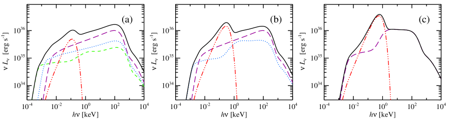
Figure 5: Upper panels: geometrical evolution at state transition. Principal components are standard accretion disc (red) and inner hot flow: zone 1 (within $10R_{\rm S}$, violet), zone 2 (within $30R_{\rm S}$, blue) and zone 3 (within $100R_{\rm S}$, green). Lower panels: spectral evolution at state transition. Contribution of different zones are marked with lines: zone 1 (long-dashed), zone 2 (dotted), zone 3 (short-dashed) and thin accretion disc (three-dot-dashed). Colour coding is the same as in the upper panels. The inner radius of the truncated accretion disc changes from (a) $100R_{\rm S}$ through (b) $30R_{\rm S}$ to (c) $10R_{\rm S}$, replacing the corresponding zones of the hot flow. Spectra are obtained for the case $\Gamma_{\rm inj}=3.0$.

The turnover frequency of the synchrotron spectrum from each radius is given by equations (3) and (4). For the case with $\Gamma_{\rm inj}=2.5$ we substitute parameters of zone 1: $R=10R_{\rm S}$, $B=10^{6}$ G, $\tau=10^{-2}$ (Thomson optical depth of the high-energy tail), and power-law slopes $\beta=5/4$, $\theta=1/2$ and $p=2$ to obtain the scaling

$$\nu_{\rm t}\approx 10^{15}\left(\frac{R}{10R_{\rm S}}\right)^{-1}{\rm Hz}.$$ (13)

The similar scaling can be obtained for $\Gamma_{\rm inj}=3.0$. In order to estimate the synchrotron luminosity we substitute the calculated turnover frequency into equation (6)

$$\nu L_{\nu}\approx 2\times 10^{35}\left(\frac{R}{10R_{\rm S}}\right)^{-7/8}{\rm erg\,s}^{-1},$$ (14)

which is consistent (within a factor of 2) with the values obtained in precise numerical calculations.

The main model parameters (see Sect. 3.1) can be constrained by the data. The first four parameters ($L$, $\Gamma_{\rm inj}$, $\tau_{1}$ and $B_{1}$) can be obtained from the X-ray luminosity and spectral slope, the cut-off temperature and the slope of the $\gamma$-ray tail. The other three parameters ($\theta$, $\beta$ and $R_{\rm tr}$) can then be extracted from the OIR data: the turnover frequency (equation 3), spectral slope (equation 7) and the luminosity (equation 6).

The precise values of the minimum and maximum Lorentz factors of the injected power-law electrons do not affect much the resulting spectra as far as the electrons emitting at the self-absorption frequency remain in a power-law. We note that very similar results can be obtained by assuming most of the energy goes to heat the thermal distribution and only a small fraction goes to the power-law tail (see Appendix B.1). At the same time, the spectra of fully thermal hot flow with the same values of magnetic field are too hard to match the observations in the hard state. Assuming $B$ an order of magnitude larger in every zone would produce the spectra reasonably well describing the observed ones. OIR spectra in this case can also be described by a power law; however, the turnover frequency in every zone is higher compared to the case of hybrid electrons (see Appendix B.1 for details). Thus, in order to explain the IR points, a much larger hot-flow size is required. We also note that purely thermal models are not capable of reproducing the observed non-thermal MeV tails.

The considered model qualitatively describes the spectral properties of the hot flow. On the quantitative level, the exact slope of the X-ray spectrum and the relative OIR/X-ray luminosities may vary depending on the details of calculations. For instance, the radiative transfer effects (see Appendix B.2) harden a bit the X-ray spectra of the outer zones, while the OIR spectra are nearly unaffected. Also reducing the $H/R$ ratio leads to slightly harder X-ray spectra (see Appendix B.2), if other parameters ($L$, $\tau$ and $B$) are unchanged. Again, the OIR slope remains the same. Thus the model is rather robust in its predicted spectral properties.

3.3 State transitions

A generally accepted scenario for the hard to soft state transition involves the motion of the cold accretion disc towards the compact object (Poutanen et al., 1997; Esin et al., 1997, 1998). In this case, the role of the disc increases and it gradually replaces the synchrotron as a source of seed photons for Comptonization. We simulate this action by replacing the spectrum in the corresponding zone of the hot flow with a multicolour blackbody disc (Shakura & Sunyaev, 1973; Frank, King & Raine, 2002) of an appropriate inner radius. We take the disc truncation radius $R_{\rm tr}$ equal to the outer radius of the largest zone of the hot flow and we keep the outer disc radius at $R_{\rm d,out}=3\times 10^{4}$ $R_{\rm S}$.

The additional seed photons for Comptonization are modelled by the injection of blackbody photons with temperature corresponding to the colour temperature of disc inner radius:

$$kT_{\rm col}=2.3\left(\frac{L}{L_{\rm Edd}}\right)^{1/4}\!\!\left(\frac{3R_{\rm S}}{R_{\rm tr}}\right)^{3/4}\!\!\left(1-\sqrt{\frac{3R_{\rm S}}{R_{\rm tr}}}\right)^{1/4}\!\!\!\mbox{keV}$$ (15)

(see Table 1). Given that the transition occurs at almost constant luminosity (see Done et al., 2007), we assume the luminosity, magnetic field and Thomson optical depth of each hot-flow zone remain the same as in the hard state (see Table 1). The relative contribution of the cold disc and the hot flow in the observed spectrum depends on the inclination, which we take equal to $60\degr$. The resulting spectra are shown in Fig. 5.

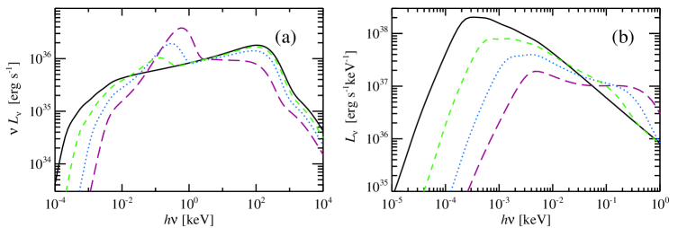
Figure 6: Spectral evolution at state transition: the pure hot-flow spectrum (solid lines), and spectra of the hot flow with the cold disc truncated at $100R_{\rm S}$ (short-dashed), $30R_{\rm S}$ (dotted), and $10R_{\rm S}$ (long-dashed). (a) spectra in $\nu L_{\nu}$ units and (b) spectra in $L_{\nu}$ units (note the different photon energy range). Here the outer disc radius is $R_{\rm d,out}=3\times 10^{4}$ $R_{\rm S}$.

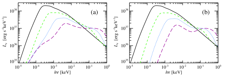
Figure 7: Same as in Fig. 6b, but for outer disc radii (a) $R_{\rm d,out}=10^{6}R_{\rm S}$ and (b) $R_{\rm d,out}=300R_{\rm S}$.

The total spectrum is now composed of synchrotron and bremsstrahlung photons, as well as Comptonized synchrotron and disc radiation. The transition between the Comptonization continua from the disc and synchrotron is reflected in the overall spectral curvature at $\sim$0.1 keV in the spectra of the largest hot-flow zone (e.g., Fig. 5a, short-dashed line). It is interesting to note that spectra of the zones closer to the BH remain almost unaffected by the disc Comptonization (e.g., Fig. 5b, long-dashed line) due to small dilution factor of the disc, while in the outermost hot-flow zone the cold disc is the dominant source of seed photons. The cool disc luminosity grows when it moves towards the BH and its photons are much more energetic than those provided by the synchrotron mechanism; thus, the X-ray spectrum softens as the transition proceeds. Once the truncation radius decreases to $10R_{\rm S}$, the spectrum becomes a combination of the disc and non-thermal synchrotron, resulting in a softer spectrum with $\alpha\approx-1$. As the outburst proceeds, the outer regions of the hot flow collapse (hours to days before the noticeable X-ray state transition) leading to a dramatic drop in luminosity at $\sim$0.1 eV. The turnover frequency increases and the OIR spectrum becomes harder (see Fig. 6). Relatively small changes occur around $E\sim 30$ eV.

Hence, one would expect fast change in the luminosity at OIR wavelengths with smaller changes in the UV. For instance, if one observes the collapse of the $100R_{\rm S}$ zone while the $30R_{\rm S}$ zone is still present, there will be huge changes at $\sim$0.5 eV, while not so significant changes at $\sim$2 eV. The opposite is expected during the soft-to-hard state transition: when the disc recedes, the hot flow occupies larger and larger radii and its synchrotron luminosity increases earlier at shorter wavelengths.

Fig. 6(b) shows the $L_{\nu}$ spectra in more details. Here we see that the pure hot-flow spectrum below the cut-off in the IR band is a power-law with index $\alpha=5/2$ corresponding to the optically thick non-thermal synchrotron. We note that such hard spectrum is obtained under the assumption of an absence of the hot flow – disc overlap, i.e. that at distances larger than the hot-flow outer radius the electron density is zero. In reality, a corona may exist atop of the cold disc, thus a gradual transition from the hot flow to the cold accretion disc is expected leading to the much more gradual turnover of the OIR spectrum.

Fig. 7 illustrates possible spectral features appearing for different sizes of the outer disc radius. We see that the hot flow completely dominates the spectrum below $\sim$10 eV if its size is larger than $100R_{\rm S}$. In this case, the exact value of $R_{\rm d,out}$ does not play any role (unless reprocessing in the outer disc starts to be important, see Sect. 4.1.4). The largest changes occur for smaller truncation radius and large $R_{\rm d,out}=10^{6}R_{\rm S}$. For such large discs (see Fig. 7a), radiation in the far IR is dominated by the Rayleigh-Jeans part of the spectrum from the outer cold disc. The UV radiation is mostly produced at the inner disc edge. Synchrotron from the hot flow is still important in the optical.

4 Comparison with observations

In the present work we considered an inhomogeneous hot accretion flow model for the broadband spectra of the accreting BHs. In the hard state, when the standard cold disc is truncated at a large radius, the central hot region is radiating mostly via thermal Comptonization of the non-thermal synchrotron photons. Hot flow extending over a large range of radii produces a power-law-like flat spectrum in the OIR range.

In the soft state, the cold disc moves in, brightens and takes over as a source of seed soft photons for Comptonization. This effectively reduces the role of synchrotron radiation in electron cooling. At the same time, the reduction of the size of the emitting region results in an increase of the synchrotron self-absorption frequency, making the synchrotron emission in the IR band negligible.

The scenario considered in this work is capable of reproducing the broadband spectra from the IR to the gamma-rays of BHs in all spectral states. However, the spectral data alone are not capable of distinguishing among various models and they have to be considered together with other sources of information (e.g. timing and polarization). Below we will discuss in details various properties of the developed hot-flow model and compare them to observations. We also compare our model to the popular jet scenario.

4.1 Hard state

4.1.1 X-ray spectrum and variability

In our model the X-ray spectrum is dominated by the Comptonization continuum from the innermost zone where most of the gravitational energy is dissipated. In the X-ray range it can generally be described by a power law. Outer zones of the hot flow have softer spectra, because of a larger role of non-thermal synchrotron and the increasing amount of the cold disc photons. The overall spectrum is thus slightly concave. Such spectra are consistent with those observed from the BHBs. For example, the best studied BH, Cyg X-1, clearly has a concave spectrum (Frontera et al., 2001a) that can be fitted with two Comptonization continua (Ibragimov et al., 2005).

A larger contribution from the outer zones to the soft X-rays should be reflected in the variability properties. Assuming that variability is produced by propagation of fluctuations in the mass accretion rate through the disc (Lyubarskii, 1997; Kotov et al., 2001), we expect an increase in the variability amplitude for higher photon energies at higher Fourier frequencies, which is indeed observed (Nowak et al., 1999a). The autocorrelation function of soft X-rays in our model is expected to be wider than that of the hard X-rays, consistent with what is measured in Cyg X-1 (Maccarone et al., 2000). The same effect is more obviously seen in the Fourier-frequency-resolved spectra (Revnivtsev, Gilfanov & Churazov, 1999; Gilfanov, Churazov & Revnivtsev, 2000), which are softer and have larger reflection amplitude at low Fourier frequencies. This implies that the outer zones of the hot flow (which are closer to the cold reflecting medium) give a relatively larger contribution to the soft X-ray flux than to the hard X-rays. The reduction of the equivalent width of the 6.4 keV Fe line in the frequency-resolved spectra above 1 Hz suggests that the cold disc truncation radius is of the order of 100 $R_{\rm S}$ (Revnivtsev et al., 1999; Gilfanov et al., 2000), further supporting our scenario. Similarly, even larger inner radii of the cold disc were measured in the low-extinction BH transient XTE J1118+480 (Esin et al., 2001; Chaty et al., 2003).

Another important finding is that the harder X-rays are delayed with respect to the soft X-rays (Nowak et al. 1999a; Nowak, Wilms & Dove 1999b). The large values of these hard time lags and their frequency-dependence $f^{-1}$ can naturally be explained by spectral pivoting of a power-law-like spectrum (Poutanen & Fabian, 1999; Poutanen, 2001). The spectral evolution can arise when the accretion rate fluctuations propagate towards the BH into the zone with harder spectra (Kotov et al., 2001), again consistent with our multizone hot-flow model.

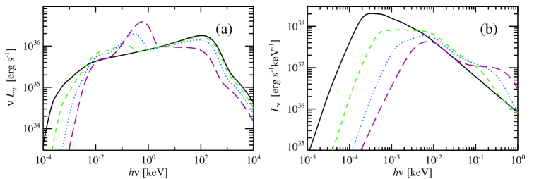
Figure 8: Same as in Fig. 6, but with the additional contribution from the irradiated accretion disc.

4.1.2 OIR excesses and flat spectra

The OIR excesses above the standard disc spectrum were reported in a number of sources: XTE J1859+226 (Hynes et al., 2002), XTE J1118+480 (Hannikainen et al., 2000; Esin et al., 2001; Chaty et al., 2003), GX 339–4 (e.g., Gandhi et al., 2011; Shidatsu et al., 2011), A0620–00 (Gallo et al., 2007), SWIFT J1753.5–0127 (Chiang et al., 2010), V404 Cyg (Hynes et al., 2009a). In our model, the OIR spectrum consists of two components (Fig. 5): one comes from the multicolour accretion disc and another from the hot flow. The relative role of these components varies with the wavelength (Figs 6 and 7). The disc spectrum is hard in the OIR band, while the non-thermal synchrotron from the hot flow is typically softer with $\alpha_{\rm OIR}\sim 0$. The second component thus produces an excess emission.

In many cases the contribution of the non-thermal component is rather small compared to the disc, and it can be seen only as the IR excess. On the other hand, sometimes the synchrotron component dominates, which results in an almost pure power-law OIR spectrum. A good example is XTE J1118+480, where the spectral index $\alpha_{\rm OIR}=-0.15$ was measured (Chaty et al., 2003). This spectral index can be reproduced in our model, for example, with parameters $\theta=0.5$, $p=2.0$ and $\beta=5/4$ (Fig. 3 illustrates this case).

4.1.3 Optical/X-ray cross-correlation

In recent years, a number of simultaneous optical(IR,UV)/X-ray observations with high time resolution were performed (Kanbach et al., 2001; Hynes et al., 2003; Gandhi et al., 2008; Hynes et al., 2009b; Durant et al., 2011), all revealing the intrinsic connection of the two light curves on subsecond time-scales. The computed CCF have a complicated shape with a dip in the optical light curve preceding the X-ray peak (the so-called precognition dip), together with an optical peak lagging the X-rays.

The behaviour can be explained if the optical emission consists of two components: one coming from the synchrotron in the hot flow and another from reprocessed X-ray emission (Veledina et al., 2011a). Increase of the mass accretion rate causes an increase in the X-ray luminosity and affects the parameters of the hot flow, leading to a higher synchrotron self-absorption. The latter results in a drop of the optical emission, therefore these two energy bands appear anticorrelated. This is reflected in the negative CCF with the shape resembling that of the X-ray autocorrelation function. On the other hand, the reprocessed radiation is delayed and smeared, giving rise to a CCF peaking at positive lags (optical delay). The combined CCF has a complicated shape consistent with the data. From the point of view of the multizone consideration, with a small increase of the mass accretion rate the cool disc moves inwards and causes the collapse of the hot flow at large radii. Thus, the suppression of the OIR emission with increasing X-ray radiation is also expected in this scenario.

A different, one-peak structure of the IR/X-ray CCF was found in GX 339–4 (Casella et al., 2010), suggesting the hot flow was not the dominant source of the correlated variability during their observations. However, it might still give significant contribution to the constant flux component, but less to the varying component, and therefore would not be detected in the timing analysis. As it can be seen from Figs 3 and 4, the zones giving major contribution to the IR wavelengths do not contribute much to the X-rays. Therefore, the fraction of the correlated variability coming from these regions is expected to be small, and another source (likely the jet emission, as suggested in Casella et al. 2010) might be responsible for the shape of the CCF. We also note that large amplitude of fluctuations in the IR light-curve suggests that the source of correlated variability is also dominating over the constant flux component.

The optical correlation with the X-rays was also detected in the quiescent state of V404 Cyg (Hynes et al., 2009a), while no clear radio/X-ray (nor radio/optical) correlation was found on the time-scales of hours, again suggesting the radio and optical/X-ray emission are produced by the different components.

4.1.4 Irradiation of the cold disc

The X-ray radiation from the hot flow can be intercepted and reprocessed in the cold disc. The irradiation strongly depends on the disc outer radius and the disc shape. The larger is $R_{\rm d,out}$, the cooler can be this emission. The more flared is the disc, the larger is the reprocessed luminosity, which typically is expected to give significant contribution to the OIR band, exceeding the viscous disc luminosity at these energies (Shakura & Sunyaev, 1973). Presence of the irradiated disc can be also reflected in the X-ray time-lags (see Poutanen, 2002, and reference therein) and in the optical/X-ray CCF (Veledina et al., 2011a). Its signatures are also seen in the spectrum (e.g., Hynes et al., 2002; Gierliński et al., 2009).

For typical parameters of LMXBs with the disc size of $10^{11}$ cm, the X-ray luminosity of $10^{37}$ erg s^-1 and 10 per cent reprocessing efficiency, the temperature of the outer disc is about 1.2 eV. For an illustration, we have added the emission from the irradiated discs to our hot-flow spectra (see Fig. 8). Following Cunningham (1976), we assumed the following dependence of the effective temperature on radius

$$kT_{\rm irr}=1.2\left(\frac{R}{R_{\rm d,out}}\right)^{-3/7}\mbox{eV}$$ (16)

and the outer disc radius of $R_{\rm d,out}=10^{11}$ cm.

As can be seen in Fig. 8, for typical parameters of the BHBs the spectrum of the irradiated disc peaks around 5 eV and has a Rayleigh-Jeans-like tail with $\alpha\sim 2$ in the OIR. If the inner hot-flow size exceeds 30–100 $R_{\rm S}$, its synchrotron emission will dominate over the reprocessing below $\sim$1 eV. We do not expect much of reprocessed emission below 0.5 eV, except for the large-period systems (similar to V404 Cyg and GRS 1915+105). Therefore, at sufficiently long wavelengths in scenario of Veledina et al. (2011a) we expect the IR/X-ray cross-correlation function to have only the dip, with no peak. The overall spectral shape is complex, with a number of bumps corresponding to the standard disc (above $\sim$100 eV), the irradiated disc and synchrotron from the hot flow (in the 1–10 eV range). A hardening of the spectrum observed in GX 339–4 at $\sim$2–3 eV (Buxton et al., 2012; Dinçer et al., 2012; Rahoui et al., 2012) can be due to a transition from the hot flow to the irradiated disc spectrum.

4.2 State transition

4.2.1 Broadband spectral evolution at state transition

During the hard-to-soft state transition the outer zones of the hot flow gradually collapse. This leads to a drop in luminosity at longer wavelengths preceding the subsequent drop at shorter wavelengths. The corresponding time delay between sharp luminosity changes at different wavelengths corresponds to the viscous time-scale of the cold disc between the corresponding radii and, depending on the separation of the wavelengths and accretion parameters, can be as short as hours (e.g., if one observes in different optical filters) and as long as a few days (e.g., IR and UV). The dramatic changes in $V$, $R$ and $I$ bands were detected, e.g. in GX 339–4 during the rising phase of the 2010 outburst (Cadolle Bel et al., 2011); however, the time resolution of the light-curves does not allow to judge on the exact time of flux quenching at different wavelengths. A much more gradual decrease of the UV flux before the X-ray spectral transition (Yan & Yu, 2012) is in principle consistent with our model if one also considers contribution from the irradiated disc (e.g., as in Fig. 8: gradual decrease at $\sim$10 eV, with sharp drop at $\sim$1 eV). During the reverse (soft-to-hard) transition, the fast luminosity increase at shorter wavelengths is expected to occur earlier than at longer wavelengths, and the corresponding time delays are expected to be larger than in the rising phase, as was seen in the 2005 outburst decay of GX 339–4 (Coriat et al., 2009).

Recently, the entire transition of the BH transient XTE J1550–564 from hard to the soft state and back was monitored in the $V$, $I$ and $H$ filters (Russell et al., 2011). Just before the X-ray spectral transition as well as after the reverse transition, significant colour variations occurred, as indicated by the rapid changes in the $H$ band at almost constant $V$ magnitude. In terms of our model, the observed colour change is related to the collapse/recover of a zone in the hot flow that is responsible for the $H$-band emission (see Section 3.3). As is known, the hard-soft and the soft-hard spectral transitions occur at different X-ray luminosities (e.g. Zdziarski et al., 2004). This hysteresis most probably is related to the fact that at the same luminosity the cold disc is further away from the central source on the rising phase of the outburst than on the decline. According to our model, the hysteresis has to be reflected also in the OIR spectra, namely the fast colour change should occur at a higher X-ray luminosity on the rising phase than on the decline. This is indeed observed (Russell et al., 2011).

In the soft state, the accretion disc extends to the last stable orbit, leaving no possibility for the inner hot flow to exist. However, the corona should still be present as supported by the existence of the non-thermal tails (produced by the inverse Compton scattering of the disc photons). It may also produce synchrotron radiation in the OIR band, but at a much lower level.

4.2.2 Change of the X-ray radiation mechanism

At luminosities above a few per cent of Eddington, BHBs show a strong correlation between spectral index and luminosity. At lower luminosities the trend is reversed (Sobolewska et al., 2011). Similarly, an indication of the reverse trend was detected in low-luminosity AGNs (Constantin et al., 2009). This was interpreted as a change of the source of seed photons for Comptonization from the disc photons dominating at higher luminosities to the synchrotron at lower luminosities. The anti-correlation at $L/L_{\rm Edd}\sim 10^{-3}$–$10^{-2}$ can be reproduced within a two-temperature hot accretion flow model (Niedźwiecki, Xie & Zdziarski, 2012). The whole spectral index – luminosity dependence is well explained by one-zone hybrid Comptonization model (see figs 7 and 12 in Veledina et al., 2011b). The multizone consideration presented in the current paper follows the same pattern as the one-zone model, because the X-ray spectrum is dominated by radiation from the inner zone.

4.3 Polarization

The only indication of the X-ray polarization from BHB goes back to the OSO-8 satellite (Weisskopf et al., 1977), which measured 3.1$\pm$1.7 per cent linear polarization from Cyg X-1 at 2.6 keV. Such a polarization can be produced by Compton scattering if the geometry of the X-ray emitting region is a flattened disc-like structure ($H/R\sim 0.2$ according to the calculations of Lightman & Shapiro, 1976). The number of scatterings the X-ray photons undergo depends on the electron and the seed photon temperatures. For a 100 keV plasma, photons double their energy in each scattering: hence, the disc photons of a typical energy of 0.5 keV would reach 3 keV in only three scatterings, while the synchrotron photons emitted at 10 eV require about eight scatterings. Thus even if the synchrotron photons are polarized, this information is forgotten, and the X-ray polarization is completely determined by the geometry of the medium. In our model, we considered the case of $H/R=0.5$, however, the spectral shape remains the same even for the flatter geometry (see Appendix B.2). Thus, the polarization measurements are consistent with the hot-flow model.

Recently, strong linear polarization ($\Pi=67\pm 30$ per cent) in the soft $\gamma$-rays above 400 keV was detected in Cyg X-1 with the IBIS instrument onboard INTEGRAL (Laurent et al., 2011). Similar polarization ($\Pi=76\pm 15$ per cent) was also observed with the SPI spectrometer (Jourdain et al., 2012a). The polarization angle of $40\degr-42\degr$ is about $60\degr$ away from the radio jet axis at $\approx-20\degr$ (Jourdain et al., 2012a; Zdziarski et al., 2012). Such a large polarization degree in the MeV range is extremely difficult to get in any scenario. Synchrotron jet emission from non-thermal electrons in a highly ordered magnetic field can have a large polarization degree (up to $\sim$70 per cent) in the optically thin part of the spectrum, and indeed a high polarization in the radio and the optical bands reaching 30–50 per cent is observed from extragalactic relativistic jets (Impey, Lawrence, & Tapia 1991; Wills et al. 1992; Lister 2001; Marscher et al. 2002; Ikejiri et al. 2011). However, this scenario also needs a very hard electron spectrum as well as an extreme fine-tuning to reproduce the spectral cutoff at a few MeV (Zdziarski et al., 2012). In the hot-flow scenario, the MeV photons are produced by non-thermal Compton scattering of the 100 keV photons by electrons with $\gamma$$\sim$2–4. These electrons cannot be isotropic, because no significant polarization is expected in that case (Poutanen, 1994). This then implies that they must have nearly one-dimensional motion, e.g. along the large-scale magnetic field lines threading the flow. The $60\degr$ offset of the polarization vector relative to the jet axis then implies the inclined field lines. If the measured high polarization degree is indeed real, this would put strong constraints on the physics of particle acceleration in the hot flow and the magnetic field geometry.

The polarization degree of the hot-flow radiation in the OIR band is strongly affected by the Faraday rotation. The rotation angle $\chi_{\rm F}\sim 10^{6}\tau B_{||,6}\nu_{15}^{-2}$ exceeds $10^{5}$ rad and the polarization degree is expected to be essentially zero in the optically thin part of the spectrum. In the optically thick regime, the intrinsic flow polarization (parallel to the field lines) is not more than about 10 per cent even for the ordered magnetic field and without Faraday rotation (Pacholczyk & Swihart, 1967; Ginzburg & Syrovatskii, 1969). Thus the OIR polarization is expected to be very low.

Optical and UV radiation from the cool accretion disc may also be polarized up to $\sim$11.7 per cent (parallel to the disc plane) at large inclinations, if the opacity is dominated by the electron scattering (Chandrasekhar, 1960; Sobolev, 1963). At lower energies, absorption in the atmospheric layers of the disc (Loskutov & Sobolev, 1981, 1982) and the Faraday rotation reduce the polarization degree and it can drop down to zero in the IR.

A detection of linear polarization at a few per cent level in the OIR bands in BHBs (Schultz et al. 2004; Shahbaz et al. 2008; Russell & Fender 2008; Chaty, Dubus & Raichoor 2011) is consistent with being produced either by the jet synchrotron radiation, extended photosphere of the hot flow, dust/electron scattering in the source vicinity or by the interstellar dust.

4.4 Comparison with the jet paradigm

The simplest jet model has a conical geometry with all parameters distributed as a power law with distance and with electrons having a power-law distribution in Lorentz factor (Marscher, 1977; Blandford & Königl, 1979). The magnetic field can be assumed ordered or tangled, but this only influences the polarization properties. The mathematical formulation of this model is identical to the analytical model for the hot flow considered in Sect. 2. Such simplified jet model was applied to the broadband spectra of BHBs (Markoff, Falcke & Fender, 2001). In a more realistic situation, the electron distribution would be subject to acceleration mechanisms, as well as cooling processes such as Compton, synchrotron and adiabatic (as e.g. in Pe’er & Casella, 2009; Pe’er & Markoff, 2012). However, due to a complicated physics, the energy input and the acceleration efficiency throughout the jet are generally unknown, and in the spectral models remain ad hoc functions. Thus the shape of the resulting spectra and its total energetics strongly depend on the assumptions. This disadvantage is avoided in the hot-flow models: the input energy here comes from the liberated gravitational energy, which can be estimated analytically, and the acceleration efficiency (as well as its role compared to other heating mechanisms) does not significantly affect the final spectrum. Both scenarios, however, suffer from a large number of parameters due to an absence of first principle model.

Apart from the different physical assumptions, the jet and the hot-flow models predict different spectral properties. In the simple jet model, the synchrotron spectrum consists of the optically thin part with spectral slope $\displaystyle\alpha=-(p-1)/2$ and the optically thick part (sum of contribution from different zones) with the same slope as given by equation (7). The low-energy cut-off is determined by the jet extension and falls in the radio wavelengths. In contrast, the cut-off of the hot-flow spectrum is related to the truncation radius of the disc and likely falls in the OIR band. The break energy to the optically thin part of the jet is determined by the extension of the injection zone and for X-ray binaries is expected to fall in the IR wavelengths (Heinz & Sunyaev, 2003), while in the hot-flow model the break is in the UV/optical band as determined by the size of the inner region. The jet optically thin synchrotron is sometimes claimed to extend to the X-rays, while in the hot-flow model radiation at these energies is produced in the Comptonization processes.

Let us now assess possible contribution of the jet and the hot flow to various wavelengths relying on the observed spectral properties. The X-ray spectra of BHBs have sharp cutoffs at about 100 keV that are impossible to produce by non-thermal synchrotron even if the electron distribution has an abrupt cutoff (Zdziarski et al., 2003). The hard spectra are also difficult to produce by optically thin synchrotron as this requires a very hard injection. Another question is then about the observed low level of the X-ray polarization, which is in contradiction with the theoretical expectations from the optically thin synchrotron, as well as with the levels measured in extragalactic sources. On the other hand, the X-ray spectral properties are well explained by the (nearly) thermal Comptonization in the hot flow (see Sect. 4.1.1).

Atop of the X-ray power-law, the Compton reflection and the iron line are rather often detected features. Their amplitude and its correlation with the underlying spectral shape strongly argue in favour of the small X-ray emission region and against any beamed-away radiation from the jet. The analysis of the hard state X-ray spectra of the BHB Cyg X-1 revealed that the spectra pivot at energies of 10–50 keV (Zdziarski et al., 2002). If the entire IR-to-X-ray continuum is produced by the same region (as proposed in the jet model), such pivoting would predict two orders of magnitude variations at 1 eV in the hard state, which are not observed. On the contrary, X-ray pivoting can be easily understood in the hot-flow model, where it can be produced by small variations of the cold disc radius and varying injection rate of the disc photons (see Fig. 8).

The observed fast X-ray variability and hard time lags can naturally be understood in the hot-flow model where the X-ray emitting region is small, and the lags are related to the viscous time-scale of propagating fluctuations (Kotov et al., 2001). At the same time, the lags can occur from Compton scattering delays within the jet (Kylafis et al., 2008), however, this model contradicts the observed narrowing of the auto-correlation function with energy (Maccarone et al., 2000).

The MeV tails detected in spectra of a number of hard-state BHBs are likely produced by the non-thermal electrons, either by the optically thin synchrotron emission (as in the jet) or by the inverse Compton scattering (as in the hot flow). The detailed investigation of this tail showed that it can be explained by the high-energy end of the jet synchrotron emission, however in this case one needs to assume a very hard index of the electron power-law distribution $p=1.3-1.6$, which is in conflict with standard acceleration models and observations (see Zdziarski, Lubiński & Sikora, 2012, and references therein). At the same time, the hot flow easily accounts for the MeV tails in the hard state as well as in the soft state (where it can be replaced by a corona), when the jet is quenched.

The non-thermal OIR radiation has often been interpreted as a jet emission (see review by Russell & Fender, 2009). The similarities in the IR and radio light-curves in microquasars, such as GRS 1915+105 (Fender et al., 1997), indeed favour common source of variability. However, this scenario meets substantial problems in a number of other sources. For instance, in some systems the jet broken power-law model, normalized to fit the radio fluxes, significantly underpredicts the optical luminosity even after accounting for possible irradiated disc contribution (Soleri et al., 2010; Cadolle Bel et al., 2011). Sometimes the OIR slope is different from the radio as, for example, in XTE J1118+480 the OIR spectrum with $\alpha_{\rm OIR}=-0.15$ is much softer than the radio spectrum with $\alpha_{\rm R}=0.5$ (Hynes et al., 2000; Chaty et al., 2003), but much harder than expected from the optically thin jet emission. The hot-flow scenario can reproduce the observed flat OIR spectra, at the same time the slopes in the OIR and radio do not necessarily match, as they are produced in different regions (inflow and outflow).

A rather low OIR polarization (at most a few per cent) observed in BHBs is clearly much below the high polarization observed in many extragalactic jets. On the other hand, certain types of objects, the so-called compact steep-spectrum and gigahertz peaked-spectrum radio sources, demonstrate similarly small polarization levels (0.2 and up to 7 per cent, respectively, O’Dea 1998). However, the (rest-frame) break frequency measured in these objects is quite low; thus, in the X-ray binary jets, as expected from the scaling laws the break frequency is in the (sub-) millimeter range.

The two models make different predictions for changes of the OIR spectrum during the state transitions. In the hot-flow scenario, the spectrum gradually hardens at hard-to-soft transition on the time-scales of days to weeks, corresponding to the typical time-scales on which the cold accretion disc evolves. It softens again at the reverse transition. On the other hand, one would not expect systematic changes of the jet spectral slope, as any fluctuations would propagate through the jet on time-scales of hours, much shorter than the state transition. However, if the jet power is gradually decreasing at the transition, then the dependence of the turnover frequency on the mass accretion rate suggests that $\nu_{\rm t}$ is also decreasing (Heinz & Sunyaev, 2003). Thus, the jet scenario predicts softening of the OIR non-thermal spectrum at hard to soft state transition and hardening at the reverse transition, opposite to the hot-flow scenario.

In reality, the OIR emission can contain contributions from a number of components: the hot flow, the jet, and the cold accretion disc (likely irradiated). It is also possible that in some sources there is a dip in the microwave band, where the transition from the radio jet to the hot flow occurs. The dip can be detected in the far infrared/submillimeter wavelengths, which were not systematically studied in the past. It is thus of high interest to observe at these wavelengths, especially with the available capabilities of the Atacama Large Millimeter/submillimeter Array.

5 Summary

The observed OIR flat spectra and the MeV tails evidence the significant role of non-thermal electrons in spectral formation of accreting BHBs. On the other hand, the commonly detected X-ray spectral cut-offs at $\sim$100 keV can be produced only by thermal particles. Whether these two populations belong to one component or originate from completely different places is debated. We present a model, in which the entire infrared to X-ray/$\gamma$-ray continuum is produced by one component, the inhomogeneous hot accretion flow, present in the vicinity of compact object. The difference from the earlier studied hot geometrically thick optically thin flows is that the steady-state electron distribution in our model is hybrid, i.e. Maxwellian with a weak high-energy tail.

The X-ray spectra in our model are dominated by the radiation of the innermost regions of the hot flow. For this reason, the model inherits the advantages of the one-zone synchrotron self-Compton model (Malzac & Belmont, 2009; Poutanen & Vurm, 2009) that explains well the X-ray spectral properties of BHB in their hard state, such as

1. stable spectra with photon index $\Gamma\sim$1.6–1.9 and the cutoff at $\sim$100 keV in the hard state,

2. low level of the X-ray polarization,

3. presence of the MeV tail in the hard state,

4. power-law-like X-ray spectra extending to a few MeV in the soft state,

5. softening of the X-ray spectrum with decreasing luminosity below $\sim$10${}^{-2}L_{\rm Edd}$,

6. weakness of the cold accretion disc component in the hard state, and

7. correlation between the spectral index, the reflection amplitude, the width of the iron line and the frequency of the QPO.

We show that the multizone consideration allows to understand many other observables in the context of the hot-flow model:

1. hard X-ray lags with logarithmic energy dependence,

2. concave X-ray spectrum,

3. non-thermal OIR excesses and flat spectra,

4. strong correlation between OIR and X-ray emission and a complicated shape of the CCF, and

5. a complex evolution of the OIR–UV spectrum during the state transition.

We present relevant analytical expressions to estimate the hot-flow parameters from the OIR data (see eqs 3, 7 and 6). Additional X-ray and $\gamma$-ray data are required to find a complete parameter set. However, the hot flow extent can be found from the OIR data alone under certain assumptions (eqs 13 and 14).

We compare the developed model to the popular jet scenario and show that in a number of cases the data favour the hot-flow interpretation. We encourage future observations in the far infrared and submillimeter wavelengths to provide the missing link between radio and infrared, which would allow us to determine the contribution of the two components to the OIR emission.

Appendix A Typical time-scales

A.1 Radiative versus Coulomb time-scales

The synchrotron cooling time can be calculated as (e.g. Rybicki & Lightman, 1979)

$$t_{\rm cool,s}=\frac{\gamma-1}{|\dot{\gamma}_{\rm s}|}=\frac{1}{\gamma+1}\left(\frac{4}{3}\frac{\sigma_{\rm T}U_{\rm B}}{m_{\rm e}c}\right)^{-1},$$ (17)

where $\dot{\gamma_{\rm s}}$ is synchrotron cooling rate. The cooling time for Compton scattering is similar. After a little algebra one can obtain

$$t_{\rm cool,s}\approx\frac{7.5\times 10^{-4}}{\gamma+1}\frac{R}{c\eta_{\rm B}}\left(\frac{L}{L_{\rm Edd}}\right)^{-1}\left(\frac{R}{10R_{\rm S}}\right),$$ (18)

where $\eta_{\rm B}=3U_{\rm B}/(4\pi U_{\rm rad})$ denotes the ratio of the magnetic and radiation field energy densities. The typical time-scale of electron-electron Coulomb energy exchange at the equilibrium can be estimated as (e.g. Nayakshin & Melia, 1998)

$$t_{\rm cool,Coul}=\frac{\gamma-1}{|\dot{\gamma}_{\rm Coul}|}\approx\frac{2R}{3c}\frac{\overline{\gamma}_{\rm eq}}{\tau\ln\Lambda}\frac{z^{3}}{\gamma(\gamma+1)},$$ (19)

where $z$ is the particle momentum in units of $m_{\rm e}c$, $\overline{\gamma}_{\rm eq}$ is the average Lorentz factor of the electrons in equilibrium and $\ln\Lambda$ is the Coulomb logarithm. At higher Lorentz factors the cooling is determined by radiative processes, while for lower $\gamma$ the non-radiative Coulomb collisions are dominant. The relative role of radiative and Coulomb cooling changes with radius:

$$\frac{t_{\rm cool,Coul}}{t_{\rm cool,s}}\approx 56\frac{z^{3}\eta_{\rm B}}{\gamma\tau}\left(\frac{L}{L_{\rm Edd}}\right)\left(\frac{R}{10R_{\rm S}}\right)^{-1},$$ (20)

where we used $\overline{\gamma}_{\rm eq}=1$ and $\ln\Lambda=17$. Therefore, the Coulomb exchange rates start dominating over the radiative cooling with an increasing size.

A.2 Coulomb versus accretion time-scales

We assume the photon spectra and electron distributions in each zone are in equilibrium; thus, the typical time-scales of equilibration should be much less than the dynamical time-scale at a given distance. To estimate the latter, we consider the properties of an advective hot flow, derived by Narayan & Yi (1994). Taking their radial velocity approximation, viscosity parameter 0.1 and assuming the adiabatic index 3/2 (Quataert & Narayan, 1999), we obtain the advection/accretion time

$$t_{\rm adv}\approx 20\sqrt{\frac{R^{3}}{GM}}.$$ (21)

We can compare the Coulomb (the radiative cooling is faster than Coulomb for $R\leq 100R_{\rm S}$) and advection time-scales (again, assuming $\overline{\gamma}_{\rm eq}=1$)

$$\frac{t_{\rm cool,Coul}}{t_{\rm adv}}\approx 5\times 10^{-4}\frac{\gamma}{\tau}\left(\frac{R}{10R_{\rm S}}\right)^{-1/2}.$$ (22)

Hence, for typical parameters $\gamma\sim$1–100 and $\tau\sim$0.1–1 the cooling time-scale is shorter than the advection time.

Appendix B Modifications of the original model

B.1 Non-thermal fraction

One of the main assumptions in our work is that all the energy dissipated in the flow is transferred to the electrons by acceleration, i.e. 100 per cent of the power is injected in the form of power-law electrons. In reality, many other dissipation mechanisms may play a significant role in particle heating, such as electron-proton Coulomb collisions (the main energy transfer mechanism in the advective flow models), resonant interactions with plasma waves and other collective plasma effects. These acceleration processes do not lead to power-law electron distributions; instead, the Maxwellian distribution is heated as a whole, achieving higher temperature. Thus it is important to check how robust the model is to changes in the fraction of non-thermal particles.

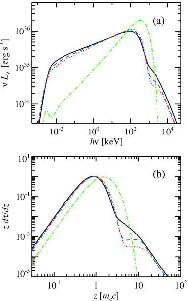
Figure 9: Effects of decreasing fraction of energy given to acceleration. Panel (a) shows resulting spectra and panel (b) gives the electron distributions. Solid black line corresponds to $f_{\rm nth}=1.0$ (same as purple long-dashed line in Fig. 4), $f_{\rm nth}=0.19$ (blue dashed), $f_{\rm nth}=0.13$ (red dotted) and $f_{\rm nth}=0$ (thermal particles, green dot-dashed). For power-law electrons the injection index $\Gamma_{\rm inj}=3.0$ was assumed.

We note that effects of decreasing non-thermal injection fraction were considered in Malzac & Belmont (2009, fig. 9), who showed that as long as this fraction is more than $\sim$30 per cent, the results are very similar. However, they fixed the minimum and the maximum Lorentz factors of the injection; thus, decreasing the non-thermal fraction would result in decreasing of normalization of the injected power-law electrons. Here we investigate the effects of decreasing non-thermal energy fraction keeping the normalization of the injected power-law constant by increasing $\gamma_{\rm min}$. As previously mentioned, the maximum Lorentz factor of accelerated electrons $\gamma_{\rm max}=10^{3}$ is assumed. The energy fraction given to power-law electrons is calculated as

$$f_{\rm nth}=\frac{\overline{(\gamma-1)}}{[\overline{(\gamma-1)}]_{\rm nth}}=\!\!(\Gamma_{\rm inj}-1)(\Gamma_{\rm inj}-2)\!\!\!\!\int\limits_{\gamma_{\rm min}}^{\gamma_{\rm max}}\!\!\!\!(\gamma-1)\gamma^{-\Gamma_{\rm inj}}d\gamma,$$ (23)

where the nominator corresponds to the energy given to accelerate the electrons between Lorentz factors $\gamma_{\rm min}$ and $\gamma_{\rm max}$, and denominator corresponds to the energy given in the purely non-thermal injection. For $\Gamma_{\rm inj}=3.0$ and $\gamma_{\rm min}=10$, the non-thermal fraction is $f_{\rm nth}=0.19$, and for $\gamma_{\rm min}=15$, $f_{\rm nth}=0.13$. The rest of dissipated energy is given to electrons via stochastic heating as described in sect. 4.1 of Vurm & Poutanen (2009). We also consider a purely thermal model, where 100 per cent of energy gained by electrons is due to stochastic heating. For an illustration, we simulated an innermost zone ($i=1$) of the hot flow with parameters described in Table 1. The results are shown in Fig. 9. We find that the resulting spectra are very similar for non-thermal fractions $f_{\rm nth}>0.1$. For even smaller $f_{\rm nth}$, the spectra are harder, but slightly adjusting other parameters (magnetic field, Thomson optical depth) we can obtain spectra, which are very close to the original purely non-thermal models. At the same time, purely thermal model has a much harder X-ray spectrum (with spectral index $\alpha=-0.43$ against $\alpha=-0.80$ for the non-thermal case) and higher equilibrium temperature ($kT_{\rm e}=213$ keV against $kT_{\rm e}=94$ keV for the non-thermal case), inconsistent with the existing X-ray data.

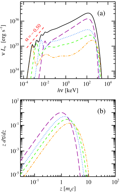
Figure 10: Same as in Figs 3 and 4, but for purely thermal electron distributions and 10 times larger magnetic field in every zone. The sharp peaks seen in the OIR are due to small number of zones considered and are not physical. The OIR spectrum is likely to be smeared and represents a power-law at these wavelengths. The red dashed line is an analytical approximation for that.

In order to describe the data with purely thermal model, a much higher magnetic field is required. Analysis of Wardziński & Zdziarski (2000) showed that purely thermal SSC cannot be the dominant radiative mechanism in majority of the X-ray binaries. However, it is interesting to test how the OIR spectrum would change in this case. Following equation 18 of Wardziński & Zdziarski (2000), the turnover frequency scales as $\nu_{\rm t}\propto B^{0.91}\tau^{0.05}T_{\rm e}^{0.95}$. As in the case of power-law electrons, it strongly depends on the magnetic field; however, the strongest dependence here is on the electron temperature. Assuming its scaling with radius $T_{\rm e}\propto R^{\kappa}$, we get

$$\nu_{\rm t}\propto R^{0.95\kappa-0.91\beta-0.05\theta},$$ (24)

which then implies that the OIR slope is

$$\alpha_{\rm OIR,th}=\frac{4+4.75\kappa-3.55\beta-0.25\theta}{1.9\kappa-1.82\beta-0.1\theta}.$$ (25)

As an illustration, we performed simulations for a purely thermal model for the whole inhomogeneous hot flow with the parameters from Table 1, except that the magnetic field in every zone was taken an order of magnitude larger, $B_{i,\rm th}=10B_{i}$. This assumption is needed to match the typical X-ray spectra in the hard state ($\alpha\sim-0.7$). However, such high $B$ is above the upper limit determined by the equipartition with protons at a virial temperature. The equilibrium electron temperature determined by the heating=cooling condition is about 20 per cent larger than in the non-thermal case (with lower $B$). The spectra and the electron distributions are shown in Fig. 10. We find that the scaling of the electron temperature with radius can be approximated with $\kappa\sim 0.3$. Substituting $\beta=1.25$ and $\theta=0.5$, gives the resulting OIR slope $\alpha_{\rm OIR,th}\approx-0.5$, in good agreement with the computed slope. Of course, no MeV emission is expected from purely thermal flows.

B.2 Geometrical and radiative transfer effects

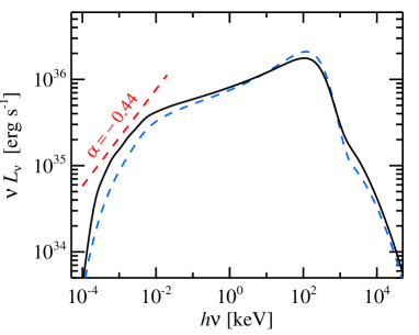
Figure 11: Spectra of a hot flow with different height-to-radius ratios. Total spectrum for $H/R=0.25$ is shown with blue dashed line and for $H/R=0.5$ (same as in Fig. 4) is shown with black solid line. The analytical approximation is shown with red dashed line.

In this section, we investigate how the assumed geometry of the flow and the interaction between the zones affect the results. Let us first check how the thickness of the hot flow affects the spectra. In order to approximate the hot flow with a number of tori, the condition of $\Delta R_{i}\approx 2H_{i}$ should be satisfied. Taking $H/R=0.25$ and using equation (8) we find $R_{i+1}\approx 5R_{i}/3$, with the innermost radius $R_{1}=3R_{\rm S}$. To cover the same distances from the BH, we now consider nine zones and scale parameters from Table 1 so that they correspond to the distance to the centre of each zone. We compare the results of calculations for $H/R=0.25$ to those for $H/R=0.5$ in Fig. 11. Due to the increase of local electron number density ($H/R$ is reduced, while optical depth was kept constant), the X-ray spectrum has become harder compared to the case $H/R=0.5$, while the OIR slopes are almost identical. The later is not surprising, as the OIR spectral shape is determined by scaling of the hot-flow parameters, rather than by their exact values in each zone.

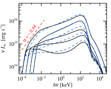
Figure 12: Spectra of the hot flow calculated accounting for the radiative transfer effects between the zones (blue dashed lines) and using local approximation (solid black lines). The upper lines represent the total spectra. Parameters of the zones are the same as in Fig. 4 and $\Gamma_{\rm inj}=3.0$ is assumed. The analytical approximation for OIR spectrum (red dashed line) is sufficiently accurate for both cases.

In our calculations we neglected the interaction between the zones and the spectrum of every zone was computed in the local approximation. However, photons from each zone can travel to the neighbouring zones. The largest effect is expected for the outer zones, because they occupy a large solid angle as viewed from the inner zones and their luminosity is smaller than that of the inner zones. The radiative transfer effects can be approximately accounted for by first computing spectra of each zone in local approximation and then by adding some fraction of the radiation escaping from each zones as an additional photon source for other zones. Luminosity coming from the $i$th zone to an adjacent $k=i\pm 1$th zone is parametrized by $\displaystyle\Omega_{ik}/(4\pi)L_{i}$, where $\Omega_{ik}$ is the solid angle occupied by $k$th zone as seen from $i$th zone. The formalism is similar to that used to simulate the outer cold disc photon injection to the hot flow. Luminosity coming from the $i$th zone to a non-adjacent zone $j$ can be expressed as $\displaystyle\Omega_{ij}/(4\pi)L_{i}e^{-\tau_{\rm ij}}$, where $\tau_{ij}$ is the photon optical depth of the medium between zones $i$ and $j$ (energy dependent, cumulative from different processes).

The resulting spectra accounting for the radiative transfer effects are compared to those computed in local approximation in Fig. 12. The changes in the OIR slope are hardly visible. The X-ray spectra of the outer zones became now harder and the variation of the 2–10 keV spectral index is smaller $\Delta\alpha_{\rm X}\approx 0.03$ (vs. 0.08). This effect is caused by additional photons coming from the harder-spectra inner zones and scattered in the outer zones in the direction to the observer. Thus, the spectra computed in the local approximation are rather accurate and agree well with more detailed calculations.

References

- Akizuki & Fukue (2006) Akizuki C., Fukue J., 2006, PASJ, 58, 469
- Arévalo & Uttley (2006) Arévalo P., Uttley P., 2006, MNRAS, 367, 801
- Blandford & Königl (1979) Blandford R. D., Königl A., 1979, ApJ, 232, 34
- Buxton et al. (2012) Buxton M. M., Bailyn C. D., Capelo H. L., Chatterjee R., Dinçer T., Kalemci E., Tomsick J. A., 2012, AJ, 143, 130
- Cadolle Bel et al. (2007) Cadolle Bel M. et al., 2007, ApJ, 659, 549
- Cadolle Bel et al. (2011) Cadolle Bel M. et al., 2011, A&A, 534, A119
- Casella et al. (2010) Casella P. et al., 2010, MNRAS, 404, L21
- Chandrasekhar (1960) Chandrasekhar S., 1960, Radiative transfer. Dover, New York
- Chaty et al. (2011) Chaty S., Dubus G., Raichoor A., 2011, A&A, 529, A3
- Chaty et al. (2003) Chaty S., Haswell C. A., Malzac J., Hynes R. I., Shrader C. R., Cui W., 2003, MNRAS, 346, 689
- Chiang et al. (2010) Chiang C. Y., Done C., Still M., Godet O., 2010, MNRAS, 403, 1102
- Condon & Dressel (1973) Condon J. J., Dressel L. L., 1973, Ap. Letters, 15, 203
- Constantin et al. (2009) Constantin A., Green P., Aldcroft T., Kim D.-W., Haggard D., Barkhouse W., Anderson S. F., 2009, ApJ, 705, 1336
- Corbel et al. (2000) Corbel S., Fender R. P., Tzioumis A. K., Nowak M., McIntyre V., Durouchoux P., Sood R., 2000, A&A, 359, 251
- Coriat et al. (2009) Coriat M., Corbel S., Buxton M. M., Bailyn C. D., Tomsick J. A., Körding E., Kalemci E., 2009, MNRAS, 400, 123
- Cunningham (1976) Cunningham C., 1976, ApJ, 208, 534
- de Bruyn (1976) de Bruyn A. G., 1976, A&A, 52, 439
- Dermer & Schlickeiser (1993) Dermer C. D., Schlickeiser R., 1993, ApJ, 416, 458
- Di Matteo et al. (1999) Di Matteo T., Celotti A., Fabian A. C., 1999, MNRAS, 304, 809
- Dinçer et al. (2012) Dinçer T., Kalemci E., Buxton M. M., Bailyn C. D., Tomsick J. A., Corbel S., 2012, ApJ, 753, 55
- Done et al. (2007) Done C., Gierliński M., Kubota A., 2007, A&ARv, 15, 1
- Droulans et al. (2010) Droulans R., Belmont R., Malzac J., Jourdain E., 2010, ApJ, 717, 1022
- Durant et al. (2008) Durant M., Gandhi P., Shahbaz T., Fabian A. P., Miller J., Dhillon V. S., Marsh T. R., 2008, ApJL, 682, L45
- Durant et al. (2009) Durant M., Gandhi P., Shahbaz T., Peralta H. H., Dhillon V. S., 2009, MNRAS, 392, 309
- Durant et al. (2011) Durant M. et al., 2011, MNRAS, 410, 2329
- Esin et al. (2001) Esin A. A., McClintock J. E., Drake J. J., Garcia M. R., Haswell C. A., Hynes R. I., Muno M. P., 2001, ApJ, 555, 483
- Esin et al. (1997) Esin A. A., McClintock J. E., Narayan R., 1997, ApJ, 489, 865
- Esin et al. (1998) Esin A. A., Narayan R., Cui W., Grove J. E., Zhang S.-N., 1998, ApJ, 505, 854
- Fabian et al. (1982) Fabian A. C., Guilbert P. W., Motch C., Ricketts M., Ilovaisky S. A., Chevalier C., 1982, A&A, 111, L9
- Fender (2006) Fender R., 2006, in Lewin W., van der Klis M., eds, Compact stellar X-ray sources, Cambridge Astrophysics Series, No. 39. Cambridge University Press, Cambridge, p. 381
- Fender et al. (2004) Fender R. P., Belloni T. M., Gallo E., 2004, MNRAS, 355, 1105
- Fender et al. (1999) Fender R. P., Garrington S. T., McKay D. J., Muxlow T. W. B., Pooley G. G., Spencer R. E., Stirling A. M., Waltman E. B., 1999, MNRAS, 304, 865
- Fender et al. (1997) Fender R. P., Pooley G. G., Brocksopp C., Newell S. J., 1997, MNRAS, 290, L65
- Frank et al. (2002) Frank J., King A., Raine D. J., 2002, Accretion Power in Astrophysics. Cambridge University Press, Cambridge
- Frontera et al. (2001a) Frontera F. et al., 2001a, ApJ, 546, 1027
- Frontera et al. (2001b) Frontera F. et al., 2001b, ApJ, 561, 1006
- Gallo et al. (2007) Gallo E., Migliari S., Markoff S., Tomsick J. A., Bailyn C. D., Berta S., Fender R., Miller-Jones J. C. A., 2007, ApJ, 670, 600
- Gandhi et al. (2008) Gandhi P. et al., 2008, MNRAS, 390, L29
- Gandhi et al. (2010) Gandhi P. et al., 2010, MNRAS, 407, 2166
- Gandhi et al. (2011) Gandhi P. et al., 2011, ApJL, 740, L13
- Gelino et al. (2010) Gelino D. M., Gelino C. R., Harrison T. E., 2010, ApJ, 718, 1
- Ghisellini et al. (1998) Ghisellini G., Haardt F., Svensson R., 1998, MNRAS, 297, 348
- Ghisellini et al. (1985) Ghisellini G., Maraschi L., Treves A., 1985, A&A, 146, 204
- Gierliński & Done (2003) Gierliński M., Done C., 2003, MNRAS, 342, 1083
- Gierliński et al. (2009) Gierliński M., Done C., Page K., 2009, MNRAS, 392, 1106
- Gierlinski et al. (1997) Gierlinski M., Zdziarski A. A., Done C., Johnson W. N., Ebisawa K., Ueda Y., Haardt F., Phlips B. F., 1997, MNRAS, 288, 958
- Gierliński et al. (1999) Gierliński M., Zdziarski A. A., Poutanen J., Coppi P. S., Ebisawa K., Johnson W. N., 1999, MNRAS, 309, 496
- Gilfanov (2010) Gilfanov M., 2010, in Belloni T., ed., The Jet Paradigm, Lecture Notes in Physics, Vol. 794. Springer Verlag, Berlin, p. 17
- Gilfanov et al. (1999) Gilfanov M., Churazov E., Revnivtsev M., 1999, A&A, 352, 182
- Gilfanov et al. (2000) Gilfanov M., Churazov E., Revnivtsev M., 2000, MNRAS, 316, 923
- Ginzburg & Syrovatskii (1969) Ginzburg V. L., Syrovatskii S. I., 1969, ARA&A, 7, 375
- Grove et al. (1998) Grove J. E., Johnson W. N., Kroeger R. A., McNaron-Brown K., Skibo J. G., Phlips B. F., 1998, ApJ, 500, 899
- Hannikainen et al. (2000) Hannikainen D. C., Hunstead R. W., Campbell-Wilson D., Wu K., McKay D. J., Smits D. P., Sault R. J., 2000, ApJ, 540, 521
- Heinz & Sunyaev (2003) Heinz S., Sunyaev R. A., 2003, MNRAS, 343, L59
- Hynes et al. (2009a) Hynes R. I., Bradley C. K., Rupen M., Gallo E., Fender R. P., Casares J., Zurita C., 2009a, MNRAS, 399, 2239
- Hynes et al. (2009b) Hynes R. I., Brien K. O., Mullally F., Ashcraft T., 2009b, MNRAS, 399, 281
- Hynes et al. (2002) Hynes R. I., Haswell C. A., Chaty S., Shrader C. R., Cui W., 2002, MNRAS, 331, 169
- Hynes et al. (2000) Hynes R. I., Mauche C. W., Haswell C. A., Shrader C. R., Cui W., Chaty S., 2000, ApJL, 539, L37
- Hynes et al. (2003) Hynes R. I. et al., 2003, MNRAS, 345, 292
- Hynes et al. (2006) Hynes R. I. et al., 2006, ApJ, 651, 401
- Ibragimov et al. (2005) Ibragimov A., Poutanen J., Gilfanov M., Zdziarski A. A., Shrader C. R., 2005, MNRAS, 362, 1435
- Ikejiri et al. (2011) Ikejiri Y. et al., 2011, PASJ, 63, 639
- Impey et al. (1991) Impey C. D., Lawrence C. R., Tapia S., 1991, ApJ, 375, 46
- Ingram & Done (2011) Ingram A., Done C., 2011, MNRAS, 415, 2323
- Jourdain et al. (2012a) Jourdain E., Roques J. P., Chauvin M., Clark D. J., 2012a, ApJ, 761, 27
- Jourdain et al. (2012b) Jourdain E., Roques J. P., Malzac J., 2012b, ApJ, 744, 64
- Kanbach et al. (2001) Kanbach G., Straubmeier C., Spruit H. C., Belloni T., 2001, Nature, 414, 180
- Kato et al. (2008) Kato S., Fukue J., Mineshige S., 2008, Black-Hole Accretion Disks – Towards a New Paradigm. Kyoto University Press, Kyoto
- Königl (1981) Königl A., 1981, ApJ, 243, 700
- Kotov et al. (2001) Kotov O., Churazov E., Gilfanov M., 2001, MNRAS, 327, 799
- Kylafis et al. (2008) Kylafis N. D., Papadakis I. E., Reig P., Giannios D., Pooley G. G., 2008, A&A, 489, 481
- Laurent et al. (2011) Laurent P., Rodriguez J., Wilms J., Cadolle Bel M., Pottschmidt K., Grinberg V., 2011, Science, 332, 438
- Lightman & Shapiro (1976) Lightman A. P., Shapiro S. L., 1976, ApJ, 203, 701
- Ling et al. (1997) Ling J. C. et al., 1997, ApJ, 484, 375
- Lister (2001) Lister M. L., 2001, ApJ, 562, 208
- Loskutov & Sobolev (1981) Loskutov V. M., Sobolev V. V., 1981, Astrofizika, 17, 535
- Loskutov & Sobolev (1982) Loskutov V. M., Sobolev V. V., 1982, Astrofizika, 18, 81
- Lyubarskii (1997) Lyubarskii Y. E., 1997, MNRAS, 292, 679
- Maccarone (2005) Maccarone T. J., 2005, MNRAS, 360, L68
- Maccarone et al. (2000) Maccarone T. J., Coppi P. S., Poutanen J., 2000, ApJL, 537, L107
- Malzac & Belmont (2009) Malzac J., Belmont R., 2009, MNRAS, 392, 570
- Malzac et al. (2009) Malzac J., Belmont R., Fabian A. C., 2009, MNRAS, 400, 1512
- Markoff et al. (2001) Markoff S., Falcke H., Fender R., 2001, A&A, 372, L25
- Marscher (1977) Marscher A. P., 1977, ApJ, 216, 244
- Marscher et al. (2002) Marscher A. P., Jorstad S. G., Mattox J. R., Wehrle A. E., 2002, ApJ, 577, 85
- McClintock et al. (2001) McClintock J. E. et al., 2001, ApJ, 555, 477
- McConnell et al. (1994) McConnell M. et al., 1994, ApJ, 424, 933
- McConnell et al. (2002) McConnell M. L. et al., 2002, ApJ, 572, 984
- Meier (2005) Meier D. L., 2005, ApSS, 300, 55
- Merloni et al. (2000) Merloni A., Di Matteo T., Fabian A. C., 2000, MNRAS, 318, L15
- Mirabel & Rodríguez (1994) Mirabel I. F., Rodríguez L. F., 1994, Nature, 371, 46
- Miyamoto & Kitamoto (1989) Miyamoto S., Kitamoto S., 1989, Nature, 342, 773
- Muno & Mauerhan (2006) Muno M. P., Mauerhan J., 2006, ApJL, 648, L135
- Narayan & Yi (1994) Narayan R., Yi I., 1994, ApJL, 428, L13
- Nayakshin & Melia (1998) Nayakshin S., Melia F., 1998, ApJS, 114, 269
- Niedźwiecki et al. (2012) Niedźwiecki A., Xie F.-G., Zdziarski A. A., 2012, MNRAS, 420, 1195
- Nolan et al. (1981) Nolan P. L. et al., 1981, ApJ, 246, 494
- Nowak et al. (1999a) Nowak M. A., Vaughan B. A., Wilms J., Dove J. B., Begelman M. C., 1999a, ApJ, 510, 874
- Nowak et al. (1999b) Nowak M. A., Wilms J., Dove J. B., 1999b, ApJ, 517, 355
- O’Dea (1998) O’Dea C. P., 1998, PASP, 110, 493
- Pacholczyk & Swihart (1967) Pacholczyk A. G., Swihart T. L., 1967, ApJ, 150, 647
- Pe’er & Casella (2009) Pe’er A., Casella P., 2009, ApJ, 699, 1919
- Pe’er & Markoff (2012) Pe’er A., Markoff S., 2012, ApJ, 753, 177
- Poutanen (1994) Poutanen J., 1994, ApJS, 92, 607
- Poutanen (1998) Poutanen J., 1998, in Abramowicz M. A., Björnsson G., Pringle J. E., eds, Theory of Black Hole Accretion Disks. Cambridge University Press, Cambridge, p. 100
- Poutanen (2001) Poutanen J., 2001, Adv. Sp. Res., 28, 267
- Poutanen (2002) Poutanen J., 2002, MNRAS, 332, 257
- Poutanen & Coppi (1998) Poutanen J., Coppi P. S., 1998, Phys. Scr. T, 77, 57
- Poutanen & Fabian (1999) Poutanen J., Fabian A. C., 1999, MNRAS, 306, L31
- Poutanen & Vurm (2009) Poutanen J., Vurm I., 2009, ApJL, 690, L97
- Poutanen & Zdziarski (2003) Poutanen J., Zdziarski A. A., 2003, in Durouchoux P., Fuchs Y., Rodriguez J., eds, New Views on Microquasars. Center for Space Physics, Kolkata, p. 95
- Poutanen et al. (1997) Poutanen J., Krolik J. H., Ryde F., 1997, MNRAS, 292, L21
- Priedhorsky et al. (1979) Priedhorsky W., Garmire G. P., Rothschild R., Boldt E., Serlemitsos P., Holt S., 1979, ApJ, 233, 350
- Quataert & Narayan (1999) Quataert E., Narayan R., 1999, ApJ, 520, 298
- Rahoui et al. (2012) Rahoui F. et al., 2012, MNRAS, 422, 2202
- Revnivtsev et al. (1999) Revnivtsev M., Gilfanov M., Churazov E., 1999, A&A, 347, L23
- Revnivtsev et al. (2001) Revnivtsev M., Gilfanov M., Churazov E., 2001, A&A, 380, 520
- Russell & Fender (2008) Russell D. M., Fender R. P., 2008, MNRAS, 387, 713
- Russell & Fender (2009) Russell D. M., Fender R. P., 2009, in Wachter A. D., Propst R. J., eds., Black Holes and Galaxy Formation. Nova Science Publishers, New York, p. 295
- Russell et al. (2011) Russell D. M., Maitra D., Dunn R. J. H., Fender R. P., 2011, MNRAS, 416, 2311
- Rybicki & Lightman (1979) Rybicki G. B., Lightman A. P., 1979, Radiative processes in astrophysics. New York, Wiley-Interscience
- Schultz et al. (2004) Schultz J., Hakala P., Huovelin J., 2004, Baltic Astronomy, 13, 581
- Shadmehri & Khajenabi (2005) Shadmehri M., Khajenabi F., 2005, MNRAS, 361, 719
- Shahbaz et al. (2008) Shahbaz T., Fender R. P., Watson C. A., O’Brien K., 2008, ApJ, 672, 510
- Shakura & Sunyaev (1973) Shakura N. I., Sunyaev R. A., 1973, A&A, 24, 337
- Shidatsu et al. (2011) Shidatsu M. et al., 2011, PASJ, 63, 785
- Sikora et al. (1994) Sikora M., Begelman M. C., Rees M. J., 1994, ApJ, 421, 153
- Sobolev (1963) Sobolev V. V., 1963, A treatise on radiative transfer. Van Nostrand, Princeton
- Sobolewska et al. (2011) Sobolewska M. A., Papadakis I. E., Done C., Malzac J., 2011, MNRAS, 417, 280
- Soleri et al. (2010) Soleri P. et al., 2010, MNRAS, 406, 1471
- Stern & Poutanen (2006) Stern B. E., Poutanen J., 2006, MNRAS, 372, 1217
- Uttley et al. (2011) Uttley P., Wilkinson T., Cassatella P., Wilms J., Pottschmidt K., Hanke M., Böck M., 2011, MNRAS, 414, L60
- Veledina et al. (2011a) Veledina A., Poutanen J., Vurm I., 2011a, ApJL, 737, L17
- Veledina et al. (2011b) Veledina A., Vurm I., Poutanen J., 2011b, MNRAS, 414, 3330
- Vurm & Poutanen (2009) Vurm I., Poutanen J., 2009, ApJ, 698, 293
- Wardziński & Zdziarski (2000) Wardziński G., Zdziarski A. A., 2000, MNRAS, 314, 183
- Wardziński & Zdziarski (2001) Wardziński G., Zdziarski A. A., 2001, MNRAS, 325, 963
- Weisskopf et al. (1977) Weisskopf M. C., Silver E. H., Kestenbaum H. L., Long K. S., Novick R., Wolff R. S., 1977, ApJL, 215, L65
- Wills et al. (1992) Wills B. J., Wills D., Evans, II N. J., Natta A., Thompson K. L., Breger M., Sitko M. L., 1992, ApJ, 400, 96
- Yan & Yu (2012) Yan Z., Yu W., 2012, MNRAS, 427, L11
- Zdziarski & Gierliński (2004) Zdziarski A. A., Gierliński M., 2004, Progress of Theoretical Physics Supplement, 155, 99
- Zdziarski et al. (2004) Zdziarski A. A., Gierliński M., Mikołajewska J., Wardziński G., Smith D. M., Harmon B. A., Kitamoto S., 2004, MNRAS, 351, 791
- Zdziarski et al. (2001) Zdziarski A. A., Grove J. E., Poutanen J., Rao A. R., Vadawale S. V., 2001, ApJL, 554, L45
- Zdziarski et al. (2003) Zdziarski A. A., Lubiński P., Gilfanov M., Revnivtsev M., 2003, MNRAS, 342, 355
- Zdziarski et al. (2012) Zdziarski A. A., Lubiński P., Sikora M., 2012, MNRAS, 423, 663
- Zdziarski et al. (1999) Zdziarski A. A., Lubinski P., Smith D. A., 1999, MNRAS, 303, L11
- Zdziarski et al. (1998) Zdziarski A. A., Poutanen J., Mikolajewska J., Gierlinski M., Ebisawa K., Johnson W. N., 1998, MNRAS, 301, 435
- Zdziarski et al. (2002) Zdziarski A. A., Poutanen J., Paciesas W. S., Wen L., 2002, ApJ, 578, 357