\mail

e-mail Denis.Golosov@biu.ac.il

11institutetext: 1 Department of Physics and the Resnick Institute, Bar-Ilan University, Ramat-Gan 52900, Israel
\published

XXXX

Phys. Status Solidi B, in press arXiv:1210.0185 Instability of the chiral phase and electronic ferroelectricity in the extended Falicov–Kimball model

D. I. Golosov\Ast,1
(XXXX, revised XXXX, accepted XXXX)
Abstract
\abstcol

We consider a spinless extended Falicov–Kimball model at half-filling, for the case of opposite-parity bands. Within the Hartree–Fock approach, we calculate the excitation energies in the chiral phase, which is a possible mean-field solution in the presence of a hybridisation. It is shown that the chiral phase is unstable.We then briefly review the accumulated results on stability and degeneracies of the excitonic insulator phase. Based on these, we conclude that the presence of both hybridisation and narrow-band hopping is required for electronic ferroelectricity.

keywords:
chiral phase, excitonic insulator, Falicov–Kimball model, electronic ferroelectricity.

1 Introduction.

In the mixed-valence regime of the extended Falicov–Kimball model (EFKM)[1], an excitonic insulator state is found within a broad range of parameter values[2, 3, 4, 5, 6]. When the two carrier bands involved (itinerant and nearly-localised) have opposite parities, a spontaneous electric polarisation (electronic ferroelectricity[7]) arises, provided that the off-diagonal excitonic average value $\langle c^{\dagger}_{i}d_{i}\rangle$ (induced hybridisation) is uniform and has a non-vanishing real part[2, 3, 7]. With the experimental search for electronic ferroelectricity underway[8], it is important to achieve a better theoretical understanding of this phenomenon.

One of the issues that needs clarification is the possibility of the chiral phase, characterised by a uniform imaginary $\langle c^{\dagger}_{i}d_{i}\rangle={\rm i}\Delta$ in the EFKM with a non-zero bare hybridisation. This scenario was mentioned earlier in the context of conventional semimetals[9]. Further discussion of the chiral phase for the case of EFKM can be found, e.g., in Ref. [10]. While not present on the available numerical[3] and mean-field[10] phase diagrams, this phase was reported to be stable in a one-dimensional EFKM with specific parameter values in the limit of strong interaction[11]. Below, we will address this issue within the Hartree–Fock approximation by considering the stability of the chiral phase with respect to collective excitations.

The issue of stability of the ferroelectric state is further complicated by possible degeneracies of the excitonic insulator phase[2, 3, 12]. In a real system, the electrostatic dipole-dipole interaction will tend to minimise the spontaneous polarisation $\vec{P}$, with the result that a $\vec{P}=0$ state will be selected whenever such a state appears among the degenerate ground states. This can be easily overcome by applying an external electric field $\vec{E}$, yet the net result is that spontaneous polarisation vanishes exactly (as opposed to a ferroelectric, where it may vanish only on average due to domain formation). This will be further discussed towards the end of the paper.

The Hamiltonian of the spinless Falicov–Kimball model (FKM) is given by

$${\cal H}=-\frac{t}{2}\sum_{\langle ij\rangle}\left(c^{\dagger}_{i}c_{j}+c^{\dagger}_{j}c_{i}\right)+E_{d}\sum_{i}d^{\dagger}_{i}d_{i}+U\sum_{i}c^{\dagger}_{i}d^{\dagger}_{i}d_{i}c_{i}\,.$$ (1)

Here, the operator $d^{\dagger}_{i}$ ($c^{\dagger}_{i}$) creates an electron in the localised (itinerant) band, $E_{d}$ is the bare energy of the

localised electrons, and $U$ is the on-site repulsion. It will be assumed that the hopping amplitude $t$ and the period of the ($d$-dimensional hypercubic) lattice are equal to unity. We will consider the half-filled case (one electron per site) at zero temperature.

While the excitonic mean field solution is present already for the pure FKM[13], Eq. (1), it is always unstable unless the FKM is extended by a small but finite[4, 12, 14] perturbation $\delta{\cal H}$. For the case of opposite-parity bands we write in the momentum space,

$$\delta{\cal H}=\sum_{\vec{k}}\left\{t^{\prime}\epsilon_{\vec{k}}d^{\dagger}_{\vec{k}}d_{\vec{k}}+{\rm i}V_{2}\lambda_{\vec{k}}\left(c^{\dagger}_{\vec{k}}d_{\vec{k}}-d^{\dagger}_{\vec{k}}c_{\vec{k}}\right)\right\}\,,$$ (2)

with $\epsilon_{\vec{k}}=-\sum_{\alpha=1}^{d}\cos k_{\alpha}$ and $\lambda_{\vec{k}}=-\sum_{\alpha=1}^{d}\sin k_{\alpha}$. Here, $t^{\prime}$ is the hopping amplitude in the narrow band, and the nearest-neighbour hybridisation is denoted $V_{2}$, consistent with Ref. [12]. We will now proceed with analysing the stability of the chiral state.

2 Instability of the chiral state.

The Hartree-Fock mean field equations for the excitonic chiral state in the model Eq. (12) read:

$$\Delta=\frac{1}{N}\sum_{\vec{k}}\Delta_{\vec{k}}^{\prime}\,,\,\,\,\Delta_{\vec{k}}^{\prime}\equiv-{\rm i}\langle c^{\dagger}_{\vec{k}}d_{\vec{k}}\rangle=\frac{U\Delta+V_{2}\lambda_{\vec{k}}}{\sqrt{(\xi_{{\vec{k}}}+t^{\prime}\epsilon_{\vec{k}})^{2}+4(U\Delta+V_{2}\lambda_{\vec{k}})^{2}}}$$ (3)

for the hybridisation, whereas for the narrow-band occupancy one finds:

$$n_{d}=\frac{1}{N}\sum_{\vec{k}}n^{d\,\prime}_{\vec{k}}\,,\,\,\,n^{d\,\prime}_{\vec{k}}\equiv\langle d^{\dagger}_{\vec{k}}d_{\vec{k}}\rangle=\frac{1}{2}-\frac{\xi_{{\vec{k}}}+t^{\prime}\epsilon_{\vec{k}}}{2\sqrt{(\xi_{{\vec{k}}}+t^{\prime}\epsilon_{\vec{k}})^{2}+4(U\Delta+V_{2}\lambda_{\vec{k}})^{2}}}\,,$$ (4)

where $N$ is the number of lattice sites, $\xi_{\vec{k}}=E_{rd}-\epsilon_{\vec{k}}$ and $E_{rd}=E_{d}+U(1-2n_{d})$. The notation $\Delta_{\vec{k}}$ ($n^{d}_{\vec{k}}$) is reserved for the leading-order terms in $\Delta^{\prime}_{\vec{k}}$ ($n^{d\,\prime}_{\vec{k}}$), corresponding to $V_{2}=t^{\prime}=0$, and is consistent with Ref. [12].

The mean-field parameters $\Delta$ and $n_{d}$, found from Eqs. (34), determine the quasiparticle dispersion in the filled and empty bands,

$$\varepsilon^{(1,2)}_{\vec{k}}=\frac{1}{2}\left\{E_{d}+(1+t^{\prime})\epsilon_{\vec{k}}+U\mp\sqrt{(\xi_{\vec{k}}+t^{\prime}\epsilon_{\vec{k}})^{2}+(4U\Delta+V_{2}\lambda_{\vec{k}})^{2}}\right\}\,.$$ (5)

Since $\lambda_{\vec{k}}=-\lambda_{-\vec{k}}$, we see that in the chiral phase, $\varepsilon^{(1,2)}_{\vec{k}}\neq\varepsilon^{(1,2)}_{-\vec{k}}$, due to the symmetry breaking[10]. We follow Ref. [12] in writing

$\displaystyle{\cal X}_{\vec{q}}=$ $\displaystyle\frac{1}{\sqrt{N}}\sum_{\vec{k}}\left\{F_{+}(\vec{k},\vec{q})\,c^{\dagger}_{\vec{k}}d_{\vec{k}+\vec{q}}+F_{-}(\vec{k},\vec{q})\,d^{\dagger}_{\vec{k}}c_{\vec{k}+\vec{q}}+F_{c}(\vec{k},\vec{q})\,c^{\dagger}_{\vec{k}}c_{\vec{k}+\vec{q}}+F_{d}(\vec{k},\vec{q})\,d^{\dagger}_{\vec{k}}d_{\vec{k}+\vec{q}}\right\}\,$ (6)

for a generic particle-hole excitation, and perform Hartree–Fock decoupling in the secular equation, $[{\cal X}_{\vec{q}},{\cal H}+\delta{\cal H}]{=}\omega_{\vec{q}}{\cal X}_{\vec{q}}$. This yields four linear equations for the amplitudes $F_{i}(\vec{k},\vec{q})$, viz.,

$\displaystyle{\rm i}(\omega-{\xi}_{\vec{k}}-t^{\prime}\epsilon_{\vec{k}+\vec{q}})F_{+}(\vec{k},\vec{q})+(U{\Delta}+V_{2}\lambda_{\vec{k}+\vec{q}})F_{c}(\vec{k},\vec{q})-(U{\Delta}+V_{2}\lambda_{\vec{k}})F_{d}(\vec{k},\vec{q})=U\left[A_{a}(\vec{q})+A_{b}(\vec{q})\right]\,,$ (7)
$\displaystyle{\rm i}(\omega+{\xi}_{\vec{k}+\vec{q}}+t^{\prime}\epsilon_{\vec{k}})F_{-}(\vec{k},\vec{q})+(U{\Delta}+V_{2}\lambda_{\vec{k}})F_{c}(\vec{k},\vec{q})-(U{\Delta}+V_{2}\lambda_{\vec{k}+\vec{q}})F_{d}(\vec{k},\vec{q})=U\left[A_{a}(\vec{q})-A_{b}(\vec{q})\right],$ (8)
$\displaystyle{\rm i}(U{\Delta}+V_{2}\lambda_{\vec{k}+\vec{q}})F_{+}(\vec{k},\vec{q})+{\rm i}(U{\Delta}+V_{2}\lambda_{\vec{k}})F_{-}(\vec{k},\vec{q})+(\omega+{\xi}_{\vec{k}+\vec{q}}-\xi_{\vec{k}})F_{c}(\vec{k},\vec{q})=UA_{c}(\vec{q})\,,$ (9)
$\displaystyle-{\rm i}(U{\Delta}+V_{2}\lambda_{\vec{k}})F_{+}(\vec{k},\vec{q})-{\rm i}(U{\Delta}+V_{2}\lambda_{\vec{k}+\vec{q}})F_{-}(\vec{k},\vec{q})+(\omega-t^{\prime}\epsilon_{\vec{k}+\vec{q}}+t^{\prime}\epsilon_{\vec{k}})F_{d}(\vec{k},\vec{q})=UA_{d}(\vec{q})\,,$ (10)

where the quantities $A_{i}(\vec{q})$ are defined self-consistently by

$\displaystyle A_{a}(\vec{q})$ $\displaystyle=$ $\displaystyle\frac{1}{2N}\sum_{\vec{p}}\left\{{\rm i}\left[F_{+}(\vec{p},\vec{q})-F_{-}(\vec{p},\vec{q})\right]({n}^{d\,\prime}_{\vec{p}}+{n}^{d\,\prime}_{\vec{p}+\vec{q}}-1)+\left[F_{c}(\vec{p},\vec{q})-F_{d}(\vec{p},\vec{q})\right]({\Delta}^{\prime}_{\vec{p}+\vec{q}}+{\Delta}^{\prime}_{\vec{p}})\right\}\,,$ (11)
$\displaystyle A_{b}(\vec{q})$ $\displaystyle=$ $\displaystyle\frac{1}{2N}\sum_{\vec{p}}\left\{{\rm i}\left[F_{+}(\vec{p},\vec{q})+F_{-}(\vec{p},\vec{q})\right]({n}^{d\,\prime}_{\vec{p}}+{n}^{d\,\prime}_{\vec{p}+\vec{q}}-1)+\left[F_{c}(\vec{p},\vec{q})+F_{d}(\vec{p},\vec{q})\right]({\Delta}^{\prime}_{\vec{p}+\vec{q}}-{\Delta}^{\prime}_{\vec{p}})\right\}\,,$ (12)
$\displaystyle A_{c}(\vec{q})$ $\displaystyle=$ $\displaystyle\frac{1}{N}\sum_{\vec{p}}\left\{{\rm i}F_{+}(\vec{p},\vec{q}){\Delta}^{\prime}_{\vec{p}}+{\rm i}F_{-}(\vec{p},\vec{q}){\Delta}^{\prime}_{\vec{p}+\vec{q}}+F_{d}(\vec{p},\vec{q})\left[{n}^{d\,\prime}_{\vec{p}}-{n}^{d\,\prime}_{\vec{p}+\vec{q}}\right]\right\}\,,$ (13)
$\displaystyle A_{d}(\vec{q})$ $\displaystyle=$ $\displaystyle\frac{1}{N}\sum_{\vec{p}}\left\{-{\rm i}F_{+}(\vec{p},\vec{q}){\Delta}^{\prime}_{\vec{p}+\vec{q}}-{\rm i}F_{-}(\vec{p},\vec{q}){\Delta}^{\prime}_{\vec{p}}-F_{c}(\vec{p},\vec{q})\left[{n}^{d\,\prime}_{\vec{p}}-{n}^{d\,\prime}_{\vec{p}+\vec{q}}\right]\right\}\,.$ (14)

We note the difference with Ref. [12], where the primary objective was to study the case of real $\langle c^{\dagger}_{i}d_{i}\rangle$.

Solving Eqs. (710) for $F_{i}(\vec{k},\vec{q})$ and substituting into Eqs. (1114) yields a system of four homogeneous equations for $A_{i}(\vec{q})$. It is important to note that in the case of pure FKM, $V_{2}=t^{\prime}=0$, the first of these equations is trivially satisfied at $\omega=0$ (all the coefficients vanish), and the $A_{a}$-terms in the remaining equations disappear.

The excitations spectrum, $\omega_{\vec{q}}$, is found from the compatibility condition of the homogeneous system for $A_{i}(\vec{q})$ (zero determinant). We already mentioned that in the $V_{2}=t^{\prime}=0$ case, the spectrum includes a branch which vanishes identically[12], $\omega_{\vec{q}}\equiv 0$. Physically, this is due to the local continuous degeneracy of the excitonic insulator in the pure FKM[1, 15]. This degeneracy is lifted by a small perturbation, Eq. (2), and the resultant low-energy branch of the spectrum can be obtained by expansion to first order in $t^{\prime}$ and to second order in $V_{2}$ and $\omega$. We obtain the following equation for the spectrum:

$\displaystyle D_{\omega}(\vec{q})\cdot\left(\frac{\omega}{U\Delta}\right)^{2}$ $\displaystyle+$ $\displaystyle M_{11}(\vec{q})\cdot D_{0}(\vec{q})+$ (15)
$\displaystyle+$ $\displaystyle V_{2}^{2}F(\vec{q})+\frac{\omega V_{2}}{U\Delta}G(\vec{q})=0\,.$

Here, the quantities $D_{\omega}(\vec{q})$ and $D_{0}(\vec{q})$ are defined as in Ref. [12] (where their momentum dependence is also discussed), whereas

$\displaystyle M_{11}$ $\displaystyle=$ $\displaystyle\frac{t^{\prime}(d+\epsilon_{\vec{q}})}{U\Delta^{2}Nd}\sum_{\vec{k}}\epsilon_{\vec{k}}n^{d}_{\vec{k}}+\frac{V_{2}^{2}}{N}\sum_{\vec{k}}\frac{4U\lambda_{\vec{k}}^{2}}{(\xi_{\vec{k}}^{2}+4U^{2}\Delta^{2})^{3/2}}-$ (16)
$\displaystyle-\frac{V_{2}^{2}}{U\Delta^{2}N}\sum_{\vec{k}}\frac{(\lambda_{\vec{k}+\vec{q}}-\lambda_{\vec{k}})^{2}}{\xi_{\vec{k}+\vec{q}}-\xi_{\vec{k}}}n^{d}_{\vec{k}}.$

Whilst the first term in $M_{11}$ is the same as in the case of a real $\langle c^{\dagger}_{i}d_{i}\rangle$, considered in Ref. [12], the terms which contain $V_{2}$ differ, reflecting the difference in the hybridised bandstructure. Furthermore, two new terms arise in Eq. (15), viz., the third term, containing an off-diagonal determinant $F$  [with $F(\vec{q})=F(-\vec{q})$], and the last term, which is proportional to $\omega V_{2}$ and odd in momentum, $G(\vec{q})=-G(-\vec{q})$. The latter term is due to the imaginary $\langle c^{\dagger}_{i}d_{i}\rangle$ breaking the inversion symmetry of the quasiparticle bands, Eq. (5). This in turn leads to breaking the symmetry of the collective excitation spectrum, $\omega_{\vec{q}}\neq\omega_{-\vec{q}}$, as follows from Eq. (15). While suppressing the lengthy explicit expressions for $F(\vec{q})$ and $G(\vec{q})$, we note that both quantities contain integrals of the form

$$\frac{1}{2N}\sum_{\vec{k}}\frac{\lambda_{\vec{k}+\vec{q}}-\lambda_{\vec{k}}}{\xi_{\vec{k}+\vec{q}}-\xi_{\vec{k}}}\left[f(\xi_{\vec{k}+\vec{q}})-f(\xi_{\vec{k}})\right]\,,$$

and therefore vanish at $\vec{q}\rightarrow 0$, as does the last term in Eq. (16).

For our immediate purposes, it is sufficient to notice that at $\vec{q}=0$ one obtains

$$\left(\frac{\omega_{\vec{q}}}{U\Delta}\right)^{2}=-\frac{D_{0}(\vec{q})}{D_{\omega}(\vec{q})}\cdot\frac{4UV_{2}^{2}}{N}\sum_{\vec{k}}\frac{\lambda_{\vec{k}}^{2}}{(\xi_{\vec{k}}^{2}+4U^{2}V_{2}^{2})^{3/2}}<0\,,$$ (17)

where we used the fact[12] that both $D_{0}$ and $D_{\omega}$ are negative at $\vec{q}=0$. Equation (17), which holds whether $t^{\prime}$ vanishes or not, guarantees that the chiral state is unstable at small $V_{2}\neq 0$ (this implies that the mean-field solution, corresponding to the chiral state, represents a saddle point rather than a local energy minimum).

The origin of this instability is different from that of the instability which arises[12] in the excitonic insulator state of the EFKM in the leading order in $t^{\prime}<0$. The latter instability is due to a sign change in $D_{0}(\vec{q})$ as $\vec{q}$ varies from $\vec{q}=0$ to $\vec{q}=\{\pi,\pi(,\pi)\}$; taking into account the next-order (in $t^{\prime}$) terms leads to a substitution $D_{0}\rightarrow D_{0}+D_{1}$. When the value of $|t^{\prime}|$ is not too small, $-t^{\prime}>|t^{\prime}_{\rm cr}|$, the quantity $D_{0}(\vec{q})+D_{1}(\vec{q})$ remains negative for all $\vec{q}$, resulting in a stabilisation of the excitonic insulator at $V_{2}=0$. We note that in this $V_{2}=0$, $t^{\prime}<0$ case the calculations of Ref. [12] remain valid whether $\langle c^{\dagger}_{i}d_{i}\rangle$ is real or imaginary, owing to exact symmetry of the EFKM mean-field Hamiltonian with respect to the phase of $\langle c^{\dagger}_{i}d_{i}\rangle$  [2, 3].

In the $V_{2}\neq 0$ case, on the other hand, the instability of the chiral state, Eq. (17), arises due to the sign of the $V_{2}$-containing terms in the system of equations for $A_{i}$ (i. e., to $M_{11}$, rather than $D_{0}$, being of the “wrong” sign at small $\vec{q}$). Hence even for $-t^{\prime}>|t^{\prime}_{\rm cr}|$, when the spectrum of the excitonic insulator state with imaginary $\langle c^{\dagger}_{i}d_{i}\rangle$ is stable for $V_{2}=0$, including an arbitrary small $V_{2}$ leads to an instability [since the first term on the r. h. s. of Eq. (16) vanishes at $\vec{q}=0$]. This situation is therefore expected to persist also when the higher-order (in $V_{2}$) terms are taken into account. We conclude that within the Hartree–Fock approach, the chiral state should remain unstable at least as long as the effects of $V_{2}$ can be treated perturbatively.

3 Conditions for electronic ferroelectricity.

We begin with the case of $t^{\prime}<0$ and $V_{2}=0$. Away from the symmetric case $E_{d}=0$, the excitonic insulator state is stabilised in the mixed-valence regime[2, 3, 4, 5], provided[4, 12] that $|t^{\prime}|$ is not too small, $-t^{\prime}>|t^{\prime}_{\rm cr}(E_{d})|$. A Goldstone mode is present at $\vec{q}=0$, corresponding to the $U(1)$ degeneracy of the Hamiltonian[2, 3]. The associated fluctuations do not destroy the long-range order in three dimensions, yet the ordered state breaks the symmetry of the model, Eqs. (12) with respect to the phase of the (uniform) $\langle c^{\dagger}_{i}d_{i}\rangle$, and is therefore degenerate.

We will now take into account the electrostatic effects, including both the interaction with an external electric field $\vec{E}$ and the dipole-dipole interaction. At zero temperature, the net energy takes form

$${\cal H}+\delta{\cal H}-\int_{\rm(sample)}\left(\vec{E}\cdot\vec{P}+\frac{1}{2}\vec{E}_{\rm int}\cdot\vec{P}\right)dV\,\,$$ (18)

Omitting other possible contributions (discussed in the standard literature), in the case of a uniform $\langle c^{\dagger}_{i}d_{i}\rangle$ we write for the polarisation density[2, 7],

$$\vec{P}=2\vec{\mu}{\rm Re}\left(\frac{1}{N}\sum_{\vec{k}}\langle c^{\dagger}_{\vec{k}}d_{\vec{k}}\rangle\right)$$ (19)

[when $\langle c^{\dagger}_{i}d_{i}\rangle$ is non-uniform, straightforward generalisation yields a non-uniform $\vec{P}(\vec{r})$]. The vector $\vec{\mu}$ is the interband matrix element of the dipole moment operator, and its direction is determined by the structure of the relevant orbitals. In Eq. (18), the internal electric field $\vec{E}_{\rm int}$ is the dipole field created by the polarised sample itself, hence the factor $1/2$ to avoid double counting; inside a uniformly polarised ball, $\vec{E}_{\rm int}=-4\pi\vec{P}/3$. This field differs from zero also outside the sample, and whether $\vec{P}$ is uniform or not, the contribution of the last term in the integrand in Eq. (18) to the total energy is

$$-\frac{1}{2}\int_{\rm(sample)}\vec{E}_{\rm int}\cdot\vec{P}dV=\frac{1}{8\pi}\int_{\rm(entire\,\,\,space)}{E}_{\rm int}^{2}dV$$ (20)

– a positive quantity, which for the case of a uniformly polarised sample is proportional to $P^{2}$.

At $\vec{E}=0$, ferroelectrics[16] (like ferromagnets at zero magnetic field[17]) tend to subdivide into domains in order to reduce the value of this term (which nevertheless remains positive) at the cost of slightly increasing the contribution of the microscopic part [in our case, ${\cal H}+\delta{\cal H}$]; the latter increase is due to domain walls formation. However, presently we encounter a different type of behaviour. As we shall see momentarily, it will suffice to consider the case of uniform polarisation $\vec{P}$.

In addition, we may assume that the electrostatic terms in Eq. (18) represent a small correction, so that generally one would first minimise the value of the microscopic energy, Eqs. (12), and then calculate the value of these terms for the appropriate ground state. However, in the present case, owing to the degeneracy of the microscopic Hamiltonian, the true ground state is chosen from the manifold of (microscopically) degenerate ground states (which are characterised by different values of $P$) by minimising the electrostatic contribution.

When $\vec{E}=0$, we see that (as mentioned in the Introduction) the dipole-dipole interaction will stabilise the state with a uniform imaginary $\langle c^{\dagger}_{i}d_{i}\rangle$, corresponding to zero polarisation. The electrostatic contribution to the energy then vanishes altogether, while the microscopic energy retains its minimal value. Applying a small electric field $\vec{E}$ would suffice to make $\langle c^{\dagger}_{i}d_{i}\rangle$ real and saturate $\vec{P}$. For a spherical sample, polarisation saturates at $|\vec{E}\cdot\vec{\mu}/\mu|>E_{\rm cr}$, where [cf. Eq. (18)] $E_{\rm cr}=8\pi|\mu||\langle c^{\dagger}_{i}d_{i}\rangle|/3$. At $|\vec{E}\cdot\vec{\mu}/\mu|<E_{\rm cr}$, polarisation would increase linearly with the field, while $\vec{E}_{\rm int}=-(\vec{E}\cdot\vec{\mu})\vec{\mu}/\mu^{2}$. The system will therefore possess a divergent dielectric constant, but would not show ferroelectricity.

In two dimensions the EFKM, Eqs. (12) with $V_{2}=0$, does not support the excitonic long-range order owing to the Mermin–Wagner theorem[3]. At $\vec{E}=0$, the dipole-dipole interaction will restore the long-range order (again with imaginary $\langle c^{\dagger}_{i}d_{i}\rangle$ , hence $\vec{P}=0$) for $-t^{\prime}>|t^{\prime}_{\rm cr}|$, and below a certain low critical temperature $T_{\rm dd}$.

In the $t^{\prime}=0$, $V_{2}\neq 0$ case, the excitonic insulator state can be stabilised in three dimensions (in agreement with Ref. [7]), provided[12] that $|V_{2}|>V_{2,{\rm cr}}(E_{d})$. Moreover, a uniform imaginary $\langle c^{\dagger}_{i}d_{i}\rangle$ corresponds to the (unstable) chiral state and therefore would not be selected. However at least within the mean field description there is a Goldstone mode surviving at $\vec{q}=\{\pi,\pi(,\pi)\}$, with an associated ground-state degeneracy as discussed in Ref.[12]. The effect of the dipole-dipole interaction at $\vec{E}=0$ will be that $\langle c^{\dagger}_{i}d_{i}\rangle$ will order in a checker-board fashion, and will be imaginary: $\langle c^{\dagger}_{i}d_{i}\rangle=\pm{\rm i}\Delta$. Thus, the behaviour of $\vec{P}(\vec{E})$ will be much like in the $t^{\prime}<0$, $V_{2}=0$ case (and $E_{\rm cr}$ will be expressed in the same way). This is at variance with Ref. [7], where the effects of electrostatic dipole-dipole interaction were not discussed.

Finally, in the $V_{2}\neq 0$, $t^{\prime}<0$ case the excitonic insulator state with real $\langle c^{\dagger}_{i}d_{i}\rangle$ can be stabilised, provided that at least one of $|V_{2}|$ and $t^{\prime}$ is sufficiently large[12]. There are no Goldstone modes, and as demonstrated above the chiral state (with a uniform imaginary $\langle c^{\dagger}_{i}d_{i}\rangle$) remains unstable at $t^{\prime}\neq 0$. We conclude that in this case even with the electrostatic dipole-dipole interaction taken into account, the EFKM shows a proper electronic ferroelectricity, characterised by a non-vanishing spontaneous polarisation, $\vec{P}\neq 0$ at $\vec{E}=0$ . This is in agreement with earlier results[3], obtained for a two-dimensional model.
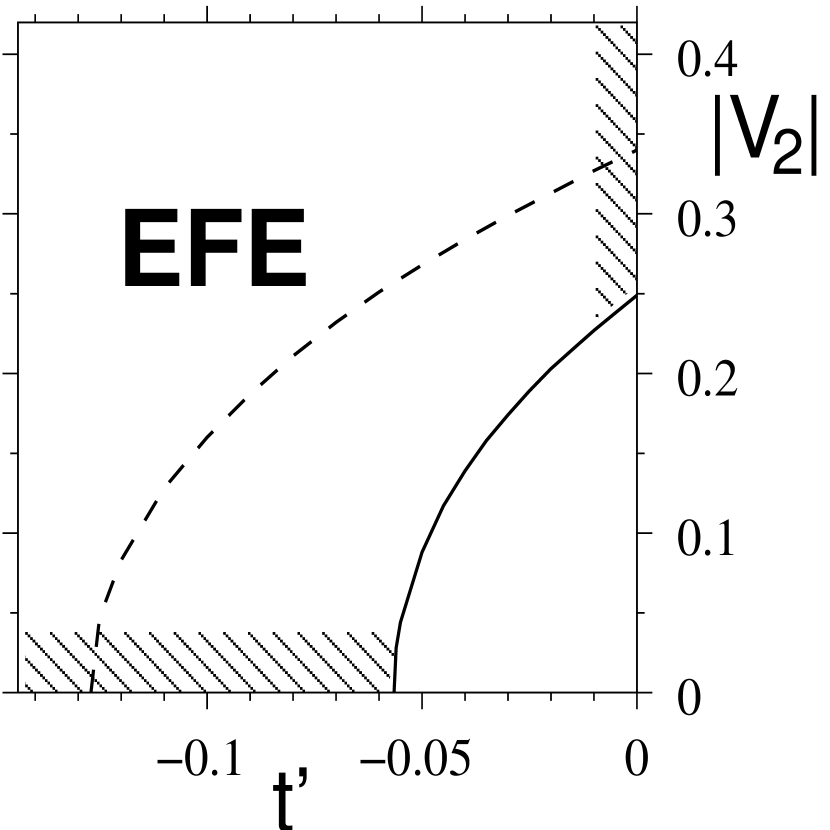
Refer to caption
Figure 1: Electronic ferroelectricity (EFE) in a two-dimensional EFKM with $U=2$ at zero temperature. For $E_{d}=0.4$ ($E_{d}=0.25$), EFE is stable above the solid (dashed) line; this line is found based on Ref. [12] as the phase boundary of a uniform excitonic insulator. When either $|V_{2}|$ or $|t^{\prime}|$ becomes too small (shown schematically by hatching; the actual width of these regions depends on the parameters of the system), the EFE is destabilised by the electrostatic dipole-dipole interaction, as discussed in the text.

When either $t^{\prime}$ or $|V_{2}|$ approaches zero, the dipole-dipole interaction would eventually destabilise the ferroelectric phase (polarisation at $\vec{E}=0$ vanishes, followed by an increase of $E_{\rm cr}$ towards the $t^{\prime}=0$ or $V_{2}=0$ value). This overall behaviour is reflected in Fig. 1, showing the stability region for electronic ferroelectricity in a two-dimensional EFKM with specific parameter values. For the case of three dimensions, similar results are expected.

4 Summary.

We verified that the chiral excitonic insulator state of the EFKM is unstable within the Hartree–Fock mean-field approach. Eliminating this possible candidate for the ground state allows to answer a general question about the possibility of electronic ferroelectricity. We find that the latter requires the presence of both hybridisation and narrow-band hopping. When only one of these is present, the dielectric constant diverges, yet the electrostatic dipole interactions preclude the formation of a spontaneous polarisation. This is due to the degeneracies of the excitonic insulator state. 

{acknowledgement}

The writer takes pleasure in thanking R. Berkovits and K. A. Kikoin for discussions. This work was supported by the Israeli Absorption Ministry.

References

  • [1] J. K. Freericks and V. Zlatić, Rev. Mod. Phys. 75, 1333 (2003), and references therein.
  • [2] C. D. Batista, Phys. Rev. Lett. 89, 166403 (2002).
  • [3] C. D. Batista, J. E. Gubernatis, J. Bonča, and H. Q. Lin, Phys. Rev. Lett. 92, 187601 (2004).
  • [4] P. Farkašovský, Phys. Rev. B77, 155130 (2008).
  • [5] G. Schneider and G. Czycholl, Eur. Phys. J. B64, 43 (2008).
  • [6] B. Zenker, D. Ihle, F. X. Bronold, and H. Fehske, Phys. Rev. B81, 115122 (2010).
  • [7] T. Portengen, Th. Östreich, and L. J. Sham, Phys. Rev. Lett. 76 3384 (1996); Phys. Rev. B54, 17452 (1996).
  • [8] C. Li, X. Zhang, Z. Cheng, and Y. Sun, Appl. Phys. Lett. 93 152103 (2008); D. S. F. Viana, R. A. M. Gotardo, L. F. Cótica, I. A. Santos, M. Olzon-Dionysio, S. D. Souza, D. Garcia, J. A. Eiras, and A. A. Coelho, J. Appl. Phys. 110 034108 (2011); P. Lunkenheimer, S. Krohns, S. Riegg, S. G. Ebbinghaus, A. Reller and A. Loidl, Eur. Phys. J. Spec. Topics 180, 61 (2010).
  • [9] B. I. Halperin and T. M. Rice, Rev. Mod. Phys. 40, 755 (1968); B. I. Halperin and T. M. Rice, in: Solid State Physics Vol. 21,, edited by F. Seitz, D. Turnbull, and H. Ehrenreich (Academic Press, New York, 1968), p. 115.
  • [10] B. Zenker, H. Fehske, and C. D. Batista, Phys. Rev. B82,165110 (2010).
  • [11] L. G. Sarasua and M. A. Continentino, Phys. Rev. B69, 073103 (2004).
  • [12] D. I. Golosov, Phys. Rev. B86, 155134 (2012).
  • [13] A. N. Kocharyan and D. I. Khomskii, Zh. Eksp. Teor. Fiz. 71, 767 (1976) [Sov. Phys. JETP 44, 404 (1976)]; H. J. Leder, Solid State Comm. 27, 579 (1978); N. Sh. Izmailyan, A. N. Kocharyan, P. S. Ovnanyan, and D. I. Khomskii, Fiz. Tverd. Tela 23, 2977 (1981) [Sov. Phys. Solid State 23, 1736 (1981)].
  • [14] G. Czycholl, Phys. Rev. B59, 2642 (1999).
  • [15] V. Subrahmanyam and M. Barma, J. Phys. C21, L19 (1988).
  • [16] J. C. Burfoot, Ferroelectrics: an Introduction to the Physical Principles (Van Nostrand, Princeton, 1967).
  • [17] A. Aharoni, Introduction to the Theory of Ferromagnetism (Oxford University Press, Oxford, 2000).