Isospin Non-Conservation in $sd$-Shell Nuclei

Abstract

The question of isospin-symmetry breaking in nuclei of the $sd$ shell is addressed. We propose a new global parametrization of the isospin-nonconserving (INC) shell-model Hamiltonian which accurately describes experimentally known isobaric mass splittings. The isospin-symmetry violating part of the Hamiltonian consists of the Coulomb interaction and effective charge-dependent forces of nuclear origin. Particular attention has been paid to the effect of the short-range correlations. The behavior of $b$ and $c$ coefficients of the isobaric-mass-multiplet equation (IMME) is explored in detail. In particular, a high-precision numerical description of the staggering effect is proposed and contribution of the charge-dependent forces to the nuclear pairing is discussed. The Hamiltonian is applied to the study of the IMME beyond a quadratic form in the $A=32$ quintet, as well as to calculation of nuclear structure corrections to superallowed $0^{+}\to 0^{+}$ Fermi $\beta$ decay, and to amplitudes of Fermi transitions to non-analogue states in $sd$-shell nuclei.

I Introduction

The isospin symmetry is one of the pivotal concepts in nuclear structure which simplifies largely many-body calculations, for example, within the nuclear shell model, and represents a useful guideline in nuclear theory. The concept is based on the charge-independence of the nucleon-nucleon (NN) interaction (invariance under any rotation in isospin space), which reflects the fact that strong proton-proton ($v^{N}_{pp}$), neutron-neutron ($v^{N}_{nn}$) and proton-neutron ($v^{N}_{pn,T=1})$ interactions are to a large extent identical. Within the isospin symmetry, a many-body nuclear Hamiltonian (without electromagnetic interactions) commutes with the isospin operator, $[H,T]=0$, and its eigenstates can be characterized by an isospin quantum number $T$ forming multiplets of $(2T+1)$ states in a few neighboring nuclei with $T_{z}=-T,\ldots,T$ (isobaric analogue states, IAS).

The charge-independence implies also a charge-symmetry of the nucleon-nucleon interaction (invariance under rotation by $180^{\circ}$ in isospace around the $T_{y}$ axis), which means the equality of $v^{N}_{pp}$ and $v^{N}_{nn}$ only, and the isospin conservation of $N=Z$ nuclei. This symmetry manifests itself in close similarity of the spectra of mirror nuclei (up to an overall shift).

Nevertheless, the isospin symmetry is only an approximate symmetry in nuclear physics mainly due to the Coulomb interaction acting between protons, but also due to the presence of charge-dependent forces of nuclear origin. The latter are understood at present to have their origin in the difference between the $u$ and $d$ quark masses and electromagnetic interactions between them Machleidt and Entem (2011). Indeed, the NN scattering data shows unambiguous evidence on the breaking of the two symmetries of the NN interaction mentioned above. First, there is a small difference between $v^{N}_{pp}$ and $v^{N}_{nn}$ (e.g., different scattering lengths in the ${}^{1}S_{0}$ channel: $a^{N}_{pp}-a^{N}_{nn}=1.65\pm 0.60$ fm Machleidt and Entem (2011)) which means the charge-symmetry breaking (or charge-asymmetry) of the NN interaction. Second, there is an even more substantial difference between $v^{N}_{pp}$ and $v^{N}_{nn}$ on one side and $v^{N}_{pn}$ on the other side (e.g., different singlet scattering lengths: $(a^{N}_{pp}+a^{N}_{nn})/2-a^{N}_{np}=5.6\pm 0.6$ fm) which corroborates the charge-independence breaking of the NN interaction. There exist also charge-dependent forces which mix the isospin of an NN system, however, we do not discuss them here. Detailed consideration and theoretical studies of these effects can be found in Refs. Miller et al. (1990); Machleidt (2001); Epelbaum et al. (2009); Machleidt and Entem (2011).

A many-body Hamiltonian containing charge-dependent forces does not commute with the isospin operator, therefore the isospin is not conserved anymore. The eigenstates of such a Hamiltonian represent a mixture of different isospin eigenstates. This is the case of explicit isospin-symmetry breaking and of isospin-mixing in nuclear states.

The degree of isospin nonconservation due to the Coulomb interaction and charge-dependent nuclear forces is small compared to nuclear effects, however, precise description of the isospin-symmetry breaking in nuclear states is crucial, when a nucleus is considered as a laboratory to test the fundamental symmetries underlying the Standard Model of the electroweak interaction. One of the important applications is the calculation of the corrections to nuclear beta decay, which arise due to the isospin-mixing in nuclear states and thus should be evaluated within a nuclear many-body model.

In particular, high-precision theoretical values of nuclear structure corrections to superallowed $0^{+}\to 0^{+}$ $\beta$-decay rates are of major interest. Combined with various radiative corrections, they serve to extract from $ft$-values of these purely Fermi transitions an absolute $\mathscr{F}t$-value of the nuclear beta decay. The constancy of $\mathscr{F}t$ for various emitters confirms the conserved vector current hypothesis (CVC) and allows one to deduce the nuclear weak-interaction coupling constant, $G_{F}$. The ratio of the latter with the weak-interaction coupling constant extracted from the muon decay gives the absolute value of $V_{ud}$, the upper-left matrix element of the Cabibbo-Kobayashi-Maskawa (CKM) matrix. The upper row of the CKM matrix is the one which provides a stringent test for the unitarity, while $V_{ud}$ being the major contributor (around ${\raise 0.73193pt\hbox{$\scriptstyle\mathtt{\sim}$}}94$%). The breakdown of the unitarity signifies a possibility of new physics beyond the Standard Model, see Ref. Towner and Hardy (2010) for a recent review.

Nowadays, $ft$-values for thirteen $0^{+}\to 0^{+}$ $\beta^{+}$ transitions among $T=1$ analogue states are known with a precision better than 0.1%. The largest uncertainty on the extracted $\mathscr{F}t$ value (which is of about 0.4%) is due to an ambiguous calculation of the nuclear structure correction Hardy and Towner (2009). Therefore, accurate theoretical description of isospin mixing in nuclear states is of primary importance.

Similarly, theoretical calculations of nuclear-structure corrections to Fermi $\beta$-decay are necessary to extract the absolute $\mathscr{F}t$ value and $V_{ud}$ matrix element from mixed Fermi/Gamow-Teller transitions in mirror $T=1/2$ nuclei Naviliat-Cuncic and Severijns (2009). Nuclear structure corrections to Gamow-Teller $\beta$-decay matrix elements are required in studies of asymmetry of Gamow-Teller $\beta$-decay rates of mirror transitions with the aim to constrain the value of the induced tensor term in the axial-vector weak current Towner (1973); Smirnova and Volpe (2003).

Apart from the nuclear structure corrections for studies of fundamental interactions, precise modelization of the Coulomb and charge-dependent nuclear forces is required to describe observed mirror energy differences Bentley and Lenzi (2007) and splittings of the isobaric multiplets, amplitudes of experimentally measured isospin-forbidden processes, such as $\beta$-delayed nucleon emission Blank and Borge (2008), Fermi $\beta$ decay to non-analogue states Hagberg et al. (1994), $E1$ transitions in self-conjugate nuclei Farnea et al. (2004) or isoscalar $E1$ component extracted from $E1$ transitions between analogue states Orlandi et al. (2009) and so on. The charge-dependent effective interaction is indispensable for understanding the structure of proton-rich nuclei with important consequences for astrophysical applications.

At the same time, accurate theoretical description of the isospin-symmetry violation within a microscopic model is a great challenge. Various approaches have been developed to deal with the problem.

The first shell-model estimations of isospin mixing are dated to the 1960’s (e.g. Refs. Blin-Stoyle and Rosina (1965); Jänecke (1969); Bertsch and Wildenthal (1973)), including their applications to the nuclear beta decay studies (see Ref. Blin-Stoyle (1969); Towner and Hardy (1973); Towner (1973) and references therein). Among the most recent work within the modern shell model, let us refer first to the study of Ormand and Brown Ormand and Brown (1985, 1989a), who constructed realistic INC effective Hamiltonians constrained by the experimental data (mass splittings of isobaric multiplets). Another approach based on the analysis of mirror energy differences in $pf$-shell nuclei was proposed by Zuker and collaborators Ref. Zuker et al. (2002) and gave a profound picture of the Coulomb effects.

It should be remembered that within the shell model, one cannot deduce completely a degree of isospin mixing in the wave function. The reason is that the Shrödinger equation is solved in the harmonic-oscillator basis within one or two oscillator shells (valence space) for valence nucleons only. An INC Hamiltonian allows to introduce the isospin-symmetry breaking in the mixing of the many-body harmonic oscillator configurations which represent Hamiltonian eigenstates. This is sufficient to get the energy shifts of isobaric multiplets due to the charge-dependent interaction. However, to get matrix elements of isospin-forbidden transitions, one has to account for the isospin-symmetry breaking beyond the model space. With this aim, one has to substitute the harmonic oscillator radial wave functions by realistic ones, since the correct asymptotics is essential. In this way, the shell model allows to predict the rates of isospin-forbidden processes which can be compared to experimental data.

Recent applications of the shell model to superallowed $\beta$ decay can be found in Refs. Ormand and Brown (1989b); Towner and Hardy (2008); Hardy and Towner (2009); Towner and Hardy (2010) and references therein, while corrections to Gamow-Teller $\beta$ decay in mirror systems have been evaluated in Refs. Towner (1973); Smirnova and Volpe (2003)). Numerous applications to the isospin-forbidden proton emission and to the structure of proton-rich nuclei can be found in the literature (e.g. Refs. Ormand and Brown (1986); Brown (1990, 1991); Ormand (1996, 1997); Cole (1996)).

The problem of the isospin-symmetry breaking was intensively undertaken in the framework of self-consistent mean-field theories within the Hartree-Fock + Tamm-Dankoff or random-phase approximation (RPA) in the 1990’s Hamamoto and Sagawa (1993); Dobaczewski and Hamamoto (1995); Colo et al. (1995); Sagawa et al. (1996). Recently, more advanced studies have been performed within the relativistic RPA approach Liang et al. (2009), as well as within the angular-momentum-projected and isospin-projected Hartree-Fock model Satula et al. (2009, 2011).

Some other many-body techniques have recently been applied to deal with isospin non-conservation. In particular, evaluation of the isospin mixing in nuclei around $N\approx Z\approx 40$ has been performed by variation-after-projection techniques on the Hartree-Fock-Bogoliubov basis with a realistic two-body force in Ref. Petrovici et al. (2008). Isospin-symmetry violation in light nuclei, applied to the case of superallowed decay of the ¹⁰C has been calculated within the ab-initio no-core shell model Caurier et al. (2002), while effects of the coupling to the continuum on the isospin mixing in weakly-bound light systems were studied in the Gamow shell-model approach Michel et al. (2010). Relation between the isospin impurities and the isovector giant monopole resonance was explored by Auerbach Auerbach (2009), with a subsequent application to the calculation of nuclear structure corrections to superallowed $\beta$ decay Auerbach (2010).

Up to now, the approaches mentioned above do not agree on the magnitude of isospin impurities in nuclear states and predict largely different values for the corrections to nuclear $\beta$ decay. Given the importance of the problematics we have revised the existing INC shell-model Hamiltonians. First, since the latest work of Ref. Ormand and Brown (1989a) there have been accumulated more experimental data and data of higher precision on the properties of isobaric multiplets (mass excess data and level schemes), on isospin-forbidden particle emission, on nuclear radii and so on. Development of the computer power and shell-model techniques allows us to access larger model spaces Caurier et al. (2005). In addition, more precise new nuclear Hamiltonians have been designed (e.g. Refs. Brown and Richter (2006); Honma et al. (2004); Nowacki and Poves (2009)), as well as new approaches to accounting for short-range correlations have been advocated Roth et al. (2010); Šimkovic et al. (2009). The purpose of this article is to present an updated set of globally-parametrized INC Hamiltonians for $sd$-shell nuclei, and to show their quantitative implication to calculations of isospin-forbidden processes in nuclei.

In Section II, we describe the formalism used for a fit of the INC interaction. Section III contains the results obtained in the $sd$ shell. In section  IV we discuss the general behavior and numerical agreement of theoretical and experimental $b$ and $c$ coefficients, as well as we reveal and study a so-called staggering phenomenon. In Section V we explore the extension of the IMME beyond the quadratic form in the lowest $A=32$ quintet. In Section VI, we present a new set of nuclear structure corrections for superallowed $0^{+}\to 0^{+}$ Fermi $\beta$ decay, as well as a few cases of Fermi transitions to non-analogue states (configuration-mixing part). The paper is summarized in the last section.

II Framework

II.1 Shell-model Formalism and Fitting Procedure

Within the nuclear shell model, the eigenproblem is solved by diagonalization of the one- plus two-body effective nuclear Hamiltonian in the basis of many-body Slater determinants constructed from the single-particle harmonic-oscillator wave functions. Since the basis dimension grows rapidly with the number of nucleons, the eigenproblem is stated only for valence nucleons in a model space containing a few (valence) orbitals above a closed-shell core. The Hamiltonian matrix thus consists of single-particle energies, $\varepsilon_{i}$, typically taken from experiment, and the two-body matrix elements (TBME’s) $V_{ijkl;J}$. Here indices $i,j,k,l$ denote full sets of quantum numbers $(nlj)$ necessary to characterize a given single-particle orbital, while $J$ denotes the total angular momentum of a coupled two-body state.

We suppose that proton-proton, neutron-neutron and proton-neutron matrix elements may all be different. Similarly, proton and neutron single-particle energies are not the same. The goal is to find an interaction which describes well both nuclear structure and the splitting of isobaric multiplets of states. In principle, an effective shell-model interaction may be derived microscopically from the bare NN force by applying a renormalization technique Hjorth-Jensen et al. (1995); Bogner et al. (2003). However, such interactions, obtained from a two-body potential only, should still be adjusted, in particular, to get correct monopole properties Poves and Zuker (1981); Caurier et al. (2005). This is done by a least-squares fit of the monopole part of the Hamiltonian or of the whole set of TBME’s to experimental data. Since the number of the matrix elements is huge, it is not feasible for the moment to get a realistic charge-dependent effective interaction in this way.

An alternative approach to the problem is first to get a reliable effective shell-model interaction in the isospin-symmetric formalism adjusted to describe experimental ground and excited-states energies. Then to add a small charge-dependent part within perturbation theory and to constrain its parameters to experimental data. Diagonalization of the total INC Hamiltonian in the harmonic oscillator basis will lead to isospin mixing.

In the $sd$ shell-model space (consisting of the $0d_{5/2}$, $1s_{1/2}$, and $0d_{3/2}$ orbitals) the most precise isospin-conserving Hamiltonians, denoted below as $H$, are the USD interaction Brown and Wildenthal (1988), as well as its two more recent versions USDA and USDB Brown and Richter (2006). First, we obtain its eigenvalues and eigenvectors:

$$H|\alpha,T,T_{z}\rangle\equiv(H_{0}+V_{0})|\alpha,T,T_{z}\rangle=E(\alpha,T)|\alpha,T,T_{z}\rangle\,.$$

Here, $\alpha=(A,J^{\pi},N_{exc},\ldots)$ denotes all other quantum numbers (except for $T$ and $T_{z}$), which are required to label a quantum state of an isobaric multiplet. $E(\alpha,T)$ is independent from $T_{z}$. $H_{0}$ is the independent-particle harmonic oscillator Hamiltonian which involves the (isoscalar) single-particle energies $\varepsilon^{(0)}_{i}=(\varepsilon^{p}_{i}+\varepsilon^{n}_{i})/2$, while $V_{0}$ stands for a two-body residual interaction in the $sd$ shell.

Then we construct a realistic isospin-symmetry violating term to get a total INC Hamiltonian. In general, we consider a charge-dependent interaction, which includes the Coulomb interaction acting between (valence) protons, and also charge-dependent forces of nuclear origin. The Coulomb interaction reads

$$V_{coul}(r)=\frac{e^{2}}{r}\,,$$ (1)

while the charge-dependent nuclear forces are represented in this work either by a set of scaled $T=1$ matrix elements of the isospin-conserving interaction $V_{0}$ (denoted as $V^{T=1}_{0}$) or by a linear combination of Yukawa-type potentials:

$$\displaystyle V_{\pi}(r) =\frac{\exp{(\mu_{\pi}r)}}{\mu_{\pi}r}\,,$$

$$\displaystyle V_{\rho}(r) =\frac{\exp{(\mu_{\rho}r)}}{\mu_{\rho}r}\,,$$ (2)

where $\mu_{\pi}=0.7$ fm^-1 and $\mu_{\rho}=3.9$ fm^-1, corresponding to the exchange of pion or $\rho$ meson, respectively, and $r$ being the relative distance between two interacting nucleons. The Coulomb interaction contributes only to the proton-proton matrix elements, while the charge-dependent nuclear forces may contribute to all nucleon-nucleon channels. Thus, we can express the charge-dependent part of the two-body interaction as

$$V= V^{pp}+V^{nn}+V^{np}$$

$$= \lambda_{coul}V_{coul}(r)$$ (3)

$$+\sum\limits_{q=pp,nn,pn(T=1)}\left(\lambda^{q}_{\pi}V^{q}_{\pi}(r)+\lambda^{q}_{\rho}V^{q}_{\rho}(r)+\lambda^{q}_{0}V^{q}_{0}\right)\,,$$

where $V^{q}_{0}$ is the same as $V_{0}^{T=1}$, while $\lambda_{coul}$, $\lambda^{q}_{\pi}$, $\lambda^{q}_{\rho}$, $\lambda^{q}_{0}$ are strength parameters characterizing the contribution of charge-dependent forces. These parameters can be established by a fit to experimental data.

The two-body charge-dependent interaction $V$ in Eq. (II.1) can alternatively be decomposed in terms of ranks 0, 1, and 2 tensors in the isospin space as

$$V=V^{(0)}+V^{(1)}+V^{(2)}\,.$$

The corresponding two-body matrix elements can be related to those in proton-neutron formalism, i.e.

$$\begin{array}[]{l}V^{(0)}_{ijkl;J}=\frac{1}{3}\left(V^{pp}_{ijkl;J}+V^{nn}_{ijkl}+V^{pn(T=1)}_{ijkl;J}\right)\,,\\ V^{(1)}_{ijkl;J}=V^{pp}_{ijkl;J}-V^{nn}_{ijkl;J}\,,\\ V^{(2)}_{ijkl;J}=V^{pp}_{ijkl;J}+V^{nn}_{ijkl;J}-2V^{pn(T=1)}_{ijkl;J}\,.\end{array}$$ (4)

In addition, the charge-dependent part of the Hamiltonian may contain a one-body term, $H^{1b}_{CD}$ of a pure isovector character, which involves the isovector single-particle energies (ISPE’s), $\varepsilon^{(1)}_{i}=\varepsilon^{p}_{i}-\varepsilon^{n}_{i}$. This term accounts for the Coulomb effects in the core nucleus. Thus the most-general charge-dependent part of the effective Hamiltonian reads

$$H_{CD}=H^{1b}_{CD}+V\,.$$

The charge-dependent part of the effective interaction is well known to be small and to be mainly of two-body type. The shift of isobaric multiplets due to the presence of charge-dependent Hamiltonian, $H_{CD}$, in lowest order of perturbation theory is given by its expectation value in the states having good isospin: $\left<\alpha,T,T_{z}\right|H_{CD}\left|\alpha,T,T_{z}\right>$. Application of the Wigner-Eckart theorem leads to the following expression:

$$\left<\alpha,T,T_{z}\right|H_{CD}\left|\alpha,T,T_{z}\right>$$

$$=E^{(0)}(\alpha,T)$$

$$+E^{(1)}(\alpha,T)T_{z}$$

$$+E^{(2)}(\alpha,T)\left[3T_{z}^{2}-T(T+1)\right]\,,$$ (5)

where the isoscalar part $V^{(0)}$ contributes only to the overall shifts of the multiplet, the isovector part $V^{(1)}$ and ISPE’s ($\varepsilon^{(1)}$) results in $E^{(1)}(\alpha,T)$, while the isotensor part $V^{(2)}$ is the only contributor to $E^{(2)}(\alpha,T)$. The latter two terms lead to the splitting of the isobaric multiplet and to the isospin mixing in the states.

Based on this assumption, Wigner showed  Wigner (1957) that a quadratic isobaric-mass-multiplet equation (IMME),

$$M(\alpha,T,T_{z})=a(\alpha,T)+b(\alpha,T)T_{z}+c(\alpha,T)T_{z}^{2}\,,$$ (6)

is sufficient to approximate the splitting of isobaric mass multiplets for a given $\alpha$, and $T$. The $a$, $b$ and $c$ are coefficients.

Since only the isovector and isotensor part of $H_{CD}$ could lead to isospin-symmetry violation (to splitting of the isobaric multiplets and to isospin mixing), we will be interested in these two terms only. Furthermore, in the fit of the nuclear TBME’s in the isospin-symmetric formalism, part of the isoscalar Coulomb term has been taken into account by an empirical correction to the experimental binding energies (see Brown and Richter (2006) and references therein). Therefore, we add to the isospin-conserving Hamiltonian a charge-dependent Hamiltonian, containing isovector (iv) and isotensor (it) terms only, namely,

$$H^{iv+it}_{CD}= \sum\limits_{q=1,2}\left(\lambda^{(q)}_{coul}V^{(q)}_{coul}(r)+\lambda^{(q)}_{\pi}V^{(q)}_{\pi}(r)+\lambda^{(q)}_{\rho}V^{(q)}_{\rho}(r)+\lambda^{(q)}_{0}V^{(q)}_{0}\right)+H^{1b}_{CD}$$

$$= \sum\limits_{q=1,2}\sum\limits_{\nu}\lambda^{(q)}_{\nu}V^{(q)}_{\nu}\,,$$ (7)

where $q$ now denotes the isotensor rank of the operators and labels the corresponding strength parameter, while the label $\nu$ is used to list all separate terms. The second line of Eq. (II.1) includes the one-body term, with $\varepsilon^{(1)}_{i}$ being the corresponding strength parameters.

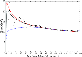
Figure 1: (Color online) Harmonic oscillator energy spacing, $\hbar\omega$: (i) Blomqvist-Molinari formula  Blomqvist and Molinari (1968) (solid black line), (ii) Blomqvist-Molinari formula with an additional scaling factor given by Eq. (3.7) of Ref. Ormand and Brown (1989a) (double-dot-dashed blue line); (iii) Blomqvist-Molinari formula refitted by Kirson  Kirson (2007) (dashed red line); (iv) $\hbar\omega$ deduced from the experimental nuclear charge radii Angeli (2004) following the procedure indicated in Ref. Kirson (2007) with $\hbar^{2}/m=41.458$ MeV.fm² (black dots). Only $A=2,\ldots,60$ is indicated.

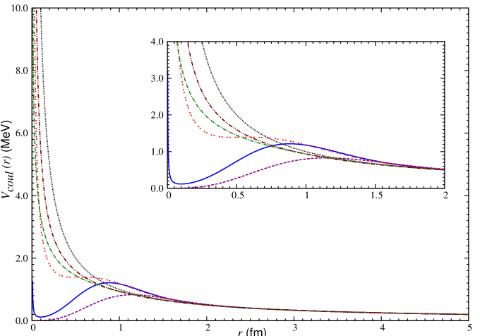
Figure 2: (Color online) $V_{coul}(r)$ without SRC (dotted black line), $V_{coul}(r)$ with proposed parameters for Jastrow type SRC on the basis of coupled-cluster calculation with CD-Bonn (double-dashed red line) or with Argonne V18 Šimkovic et al. (2009) (solid blue line), $V_{coul}(r)$ with Miller-Spencer parametrized Jastrow type SRC Miller and Spencer (1976) (dashed purple line); $V_{coul}(R^{I}_{+}(r))$ with UCOM SRC (dot-dashed green line), $V_{coul}(R^{II}_{+}(r))$ with UCOM SRC (double-dot-dashed brown line). The inset enlarges the left-hand part of this figure.

The isovector $E^{(1)}(\alpha,T)$ and isotensor $E^{(2)}(\alpha,T)$ contributions to the expectation value of $H^{iv+it}_{CD}$ (or $H_{CD}$), can be either extracted from the energy shift due to the isovector $V^{(1)}$ (or $H^{1b}_{CD}$) and isotensor $V^{(2)}$ parts of the charge-dependent Hamiltonian, respectively, or from calculations of the energy shifts of all multiplet members. Following the latter method, we represent the TBME’s of $V_{\nu}$ in terms of the proton-proton matrix elements only and then we calculate its expectation value in each state of the multiplet $E_{\nu}(\alpha,T,T_{z})=\left<\alpha,T,T_{z}\right|V_{\nu}\left|\alpha,T,T_{z}\right>$. Then, the isovector and isotensor contributions to a given multiplet of states are respectively expressed as

$$\displaystyle E^{(1)}_{\nu}(\alpha,T)= \frac{3}{T(T+1)(2T+1)}\sum\limits_{T_{z}=-T}^{T}(-T_{z})E_{\nu}(\alpha,T,T_{z})\,,$$

$$\displaystyle E^{(2)}_{\nu}(\alpha,T)= \frac{5}{T(T+1)(2T-1)(2T+1)(2T+3)}$$ (8)

$$\times\sum\limits_{T_{z}=-T}^{T}\left[3T^{2}_{z}-T(T+1)\right]E_{\nu}(\alpha,T,T_{z})\,.$$

The same method holds also for the ISPE’s. Summing over all contributions to $H_{CD}$, we get theoretical IMME $b$ and $c$ coefficients as

$$\begin{array}[]{l}b^{th}(\alpha,T)=\sum\limits_{\nu}\lambda^{(1)}_{\nu}E^{(1)}_{\nu}(\alpha,T)\,,\\ c^{th}(\alpha,T)=3\sum\limits_{\nu}\lambda^{(2)}_{\nu}E^{(2)}_{\nu}(\alpha,T)\,.\\ \end{array}$$ (9)

ISPE’s are only included into the expression for $b^{th}$ values.

To find the best strengths $\lambda^{(q)}_{\nu}$, we have performed a least-squares fit of theoretical $b^{th}$ and $c^{th}$ coefficients to experimental IMME $b$ and $c$ coefficients : $b^{exp}_{i}\pm\sigma_{i}$ ($i=1,\ldots,N_{b}$) and $c^{exp}_{j}\pm\sigma_{j}$ ($j=1,\ldots,N_{c}$). Implying that they have a Gaussian distribution, we have minimized the $\chi^{2}$ deviation (e.g., for $b$ coefficients):

$$\chi^{2}=\sum\limits_{i=1}^{N_{b}}\frac{(b^{exp}_{i}-b^{th}_{i})^{2}}{\sigma_{i}^{2}}\,,$$ (10)

with respect to the parameters $\lambda^{(1)}_{\nu}$, i.e.

$$\frac{\partial\chi^{2}}{\partial\lambda^{(1)}_{\nu}}=\frac{\partial}{\partial\lambda^{(1)}_{\nu}}\sum\limits_{i=1}^{N_{b}}\frac{(b^{exp}_{i}-b^{th}_{i})^{2}}{\sigma_{i}^{2}}=0\,,$$ (11)

which has lead us to a system of linear equations for $\lambda^{(1)}_{\nu}$:

$$\sum\limits_{i=1}^{N_{b}}\left[\frac{E^{(1)}_{\mu i}b^{exp}_{i}}{\sigma_{i}^{2}}-\sum\limits_{\nu}\frac{\lambda^{(1)}_{\nu}E^{(1)}_{\nu i}E^{(1)}_{\mu i}}{\sigma_{i}^{2}}\right]=0.$$ (12)

In matrix form this system looks as

$${\bf\Lambda W}={\bf Q}\quad{\rm or}\quad\sum\limits\Lambda_{\nu}W_{\nu\mu}=Q_{\mu}\,,$$ (13)

with

$$\displaystyle\Lambda_{\nu} =\lambda^{(1)}_{\nu}\,,$$

$$\displaystyle W_{\nu\mu} =\sum\limits_{i=1}^{N_{b}}\frac{E^{(1)}_{\nu i}E^{(1)}_{\mu_{i}}}{\sigma_{i}^{2}}\,,$$

$$\displaystyle Q_{\mu} =\sum\limits_{i=1}^{N_{b}}\frac{E^{(1)}_{\mu i}b^{exp}_{i}}{\sigma_{i}^{2}}\,.$$ (14)

Since theoretical $b$ and $c$ coefficients are linear functions of the unknown parameters $\lambda^{(q)}_{\nu}$ of Eq. (9), the fitting procedure is reduced to solving linear equations. Solution of these equations with respect to ${\bf\Lambda}$ results in a set of the most optimal strength parameters $\lambda^{(1)}_{\nu}$:

$${\bf\Lambda}={\bf QW}^{-1}\,.$$ (15)

To get uncertainties of the strength parameters found, we evaluate the root-mean-square (rms) deviation from the error matrix ${\bf W}^{-1}$ as

$$\Delta\lambda^{(1)}_{\nu}=\sqrt{\langle(\lambda^{(1)}_{\nu}-\overline{\lambda^{(1)}_{\nu}})^{2}\rangle}=\sqrt{(W^{-1})_{\nu\nu}}\,.$$ (16)

A similar procedure holds for the adjustment of $c$ coefficients.

After adjusting the interaction, we solve the eigenproblem for a thus constructed INC Hamiltonian in the proton-neutron formalism: $[H_{INC},T]\neq 0$:

$$H_{INC}|\alpha_{p},\alpha_{n}\rangle\equiv(H+H^{iv+it}_{CD})|\alpha_{p},\alpha_{n}\rangle=E|\alpha_{p},\alpha_{n}\rangle\,.$$

As a result, the Hamiltonian eigenstates do not possess good isospin quantum number anymore and thus are mixtures of different $T$ values.

The shell model diagonalization has been performed using modern version of the ANTOINE shell-model code Caurier and Nowacki (1999).

II.2 TBME’s of the Coulomb and Yukawa-Type Potentials

II.2.1 Harmonic Oscillator Parameter

The TBME’s of the Coulomb and Yukawa-type potentials Eq. (1) and Eq. (II.1), used to calculate the energy shifts, were evaluated using the harmonic-oscillator wave functions for mass $A=39$ and the subsequent scaling

$$S(A)=\left(\frac{\hbar\omega(A)}{\hbar\omega(A_{0}=39)}\right)^{1/2}.$$ (17)

In Ref. Ormand and Brown (1989a), $\hbar\omega$ was taken in its most commonly used parametrization expressed by the Blomqvist-Molinari formula  Blomqvist and Molinari (1968):

$$\hbar\omega(A)=45A^{-1/3}-25A^{-2/3}\,.$$ (18)

For the $sd$ shell, an additional scaling factor was imposed (see Eq. (3.7) in Ref. Ormand and Brown (1989a)) to improve the agreement with the data at the beginning and at the end of the $sd$ shell.

However, recent empirical values of $\hbar\omega$, derived from updated experimental nuclear charge radii in Ref. Angeli (2004), differ significantly from the values predicted by Ormand and Brown in Ref. Ormand and Brown (1989a), especially in the middle of the $sd$ shell, not considered in the latter work. The comparison is shown in Fig. 1. Some improvement is reached by a recent global parametrization of the Blomqvist-Molinari formula for the whole nuclear chart ($A=2,\ldots,248$) performed by Kirson Kirson (2007) (see Fig. 1).

We have performed a fit with both parametrizations of $\hbar\omega$, however, none of them resulted in a sufficiently low rms deviation values in our fit for $b$ and $c$ coefficients. The plausible reason is that the existing parametrizations for $\hbar\omega$ values in the $sd$ shell are not close to the values extracted from experimental nuclear charge radii. To overcome this difficulty, in the present work we have scaled the TBME’s as given by Eq. (17), directly using experimentally based values for $\hbar\omega$ values in the $sd$ shell, mentioned above and shown in Fig. 1. The ISPE’s were also evaluated for $A=39$ and then scaled as given by Eq. (17).

We remark that due to the empirical character of the $sd$-shell isospin-conserving interactions, one could calculate the TBME’s of the Coulomb and Yukawa type potentials using a more realistic basis, such as single-particle wave functions obtained from a spherical Woods-Saxon potential. This may lead to an improvement in the fit. We are currently exploring this possibility and the results will be published elsewhere.

II.2.2 Short-Range Correlations

Since the TBME’s of Coulomb or meson-exchange potentials are calculated by using harmonic-oscillator wave functions, it is important to account for the presence of short-range correlations (SRC). We have carefully studied this issue by two different methods. First, the Jastrow-type correlation function, which modifies the relative part of the harmonic-oscillator basis, $\phi_{nl}(r)$, to

$$\phi^{\prime}_{nl}(r)=\left[1+f(r)\right]\phi_{nl}(r)\,,$$

with $f(r)$ being parametrized as

$$f(r)=-\gamma e^{-\alpha r^{2}}\left(1-\beta r^{2}\right)\,.$$ (19)

Then the radial part of the TBME’s of the Coulomb and Yukawa type potentials between the modified harmonic-oscillator wave functions $\phi^{\prime}_{nl}(r)$ and $\phi^{\prime}_{n^{\prime}l}(r)$ becomes

$$\int\limits_{0}^{\infty}\phi^{\prime}_{nl}(r)v(r)\phi^{\prime}_{n^{\prime}l}(r)dr=\int\limits_{0}^{\infty}\phi_{nl}(r)v(r)\left[1+f(r)\right]^{2}\phi_{n^{\prime}l}(r)dr\,.$$ (20)

We used three different sets of parameters $\alpha$, $\beta$ and $\gamma$ in Eq. (19): those given by Miller and Spencer Miller and Spencer (1976) and two alternative sets recently proposed on the basis of coupled-cluster studies with Argonne (AV18) and CD-Bonn potentials Šimkovic et al. (2009) (see Table 1). For brevity, we will refer to the two latter sets as CD-Bonn and AV18.

Table 1: Parameters for the short-range correlation function.

	$\alpha$	$\beta$	$\gamma$
Miller-Spencer	1.10	0.68	1.00
CD-Bonn	1.52	1.88	0.46
Argonne-V18	1.59	1.45	0.92

Table 2: Ratios of Coulomb expectation values of ¹⁸Ne, ³⁸K, ³⁰S, ²⁶Mg, produced from various SRC approaches to evaluation without (w/o) SRC.

	$\left<\psi\right|V_{coul\,\textnormal{w/o SRC}}\left|\psi\right>$	$\left<\psi\right|V_{coul\,\textnormal{with SRC}}\left|\psi\right>/\left<\psi\right|V_{coul\,\textnormal{w/o SRC}}\left|\psi\right>$
	(MeV)	Miller-Spencer	CD-Bonn	Argonne V18	UCOM
Mass 18, 18Ne
$0^{+}$ g.s.	0.531	0.900	1.008	0.978	0.958
$2^{+}$	0.449	0.961	1.010	0.997	0.981
$4^{+}$	0.389	0.984	1.007	1.001	0.991
$0^{+}$	0.412	0.952	1.005	0.990	0.979
$2^{+}$	0.380	0.993	1.006	1.003	0.994
$0^{+}$	0.425	0.980	1.011	1.004	0.987
Mass 38, 38K
$0^{+}$ g.s.	16.402	0.986	1.007	1.003	0.991
$2^{+}$	16.316	0.986	1.007	1.003	0.992
Mass 30, 30S
$0^{+}$ g.s.	10.721	0.984	1.007	1.002	0.990
$2^{+}$	10.696	0.985	1.007	1.002	0.991
$2^{+}$	10.704	0.985	1.007	1.002	0.991
$1^{+}$	10.632	0.987	1.007	1.003	0.992
Mass 26, 26Mg
$0^{+}$ g.s.	2.518	0.967	1.008	0.998	0.984
$2^{+}$	2.480	0.974	1.008	1.000	0.986
$2^{+}$	2.491	0.972	1.008	0.999	0.986
$0^{+}$	2.491	0.972	1.008	0.999	0.986

Besides, we have also used another renormalization scheme following the unitary correlation operator method (UCOM) Roth et al. (2005). Since we need to correct only central operators, the UCOM reduces to the application of central correlators only, i.e. the radial matrix elements are of the form

$$\int\limits_{0}^{\infty}\phi_{n^{\prime}l}(r)v\left(R_{+}(r)\right)\phi_{nl}(r)dr\,,$$ (21)

where two different $R_{+}(r)$ functions have been used in $S=0,T=1$ and $S=1,T=1$ channels, namely,

$$R^{\rm I}_{+}(r)=r+\alpha\left(\frac{r}{\beta}\right)^{\eta}\exp\left[-\exp{\left(\frac{r}{\beta}\right)}\right]\,,$$ (22)

with $\alpha=1.3793$ fm, $\beta=0.8853$ fm, $\eta=0.3724$ in the $S=0,T=1$ channel, and

$$R^{\rm II}_{+}(r)=r+\alpha\left(1-\exp{\left(-\frac{r}{\gamma}\right)}\right)\exp\left[-\exp{\left(\frac{r}{\beta}\right)}\right]\,,$$ (23)

with $\alpha=0.5665$ fm, $\beta=1.3888$ fm, $\gamma=0.1786$ in the $S=1,T=1$ channel Roth et al. (2005).

The modifications of $V_{coul}$ brought about by different approaches to the SRC issue are shown in Fig. 2. Similar trends hold for $V_{\rho}$ and $V_{\pi}$.

Although the UCOM renormalization scheme differs from the Jastrow-type correlation functions, we can easily notice that either of the $R_{+}(r)$ functions does not strongly affect the original potentials. Somewhat stronger modifications are brought about by the CD-Bonn based parametrization. The Miller-Spencer parametrization of the correlation function induces the highest suppression of the potentials at short distances and leads to a vanishing value at $r=0$. Similar conclusions are reported in Ref. Šimkovic et al. (2008) in the context of double-beta decay studies. Strong modifications are clearly seen for AV18 as well.

To illustrate the effect from different approaches to the SRCs on the results to be discussed in the following, we present in Table 2 the ratios of the Coulomb expectation values in the ground and several low-lying excited states of a few selected nuclei from the bottom, from the top, and from the middle of the $sd$ shell-model space, i.e. ¹⁸Ne (2 valence protons), ³⁸K (2 proton holes), and ³⁰S and ²⁶Mg, respectively. The second column of Table 2 contains absolute expectation values of the bare Coulomb interaction, while the other columns show the ratios to it from Coulomb interaction expectation values which include SRC.

It is seen that the Miller-Spencer approach to SRC quenches the Coulomb matrix element (as well as that of the Yukawa $\rho$-meson exchange potential) and thus reduces Coulomb expectation values more compared to other SRC schemes. Interestingly, the CD-Bonn parametrization and in some cases the AV-18 parametrization show even a small increase of the Coulomb expectation value. Bearing this in mind, in the next section we, however, perform a fit of the INC parameters for all cited approaches to the SRCs.

III Results and Discussion

III.1 Fitting Procedure

We have followed the fitting strategy proposed in Ref. Ormand and Brown (1989a). First, we construct theoretical $b$ and $c$ coefficients Eq. (9) as described in the previous section (using experimentally based $\hbar\omega$ and accounting for the SRC by one of the above mentioned methods). Then, we separately fit them to experimental $b$ and $c$ coefficients to get the most optimal values of $\lambda^{(1)}_{\nu}$ and $\lambda^{(2)}_{\nu}$, respectively. We assume here that the isovector and isotensor Coulomb strengths are equal. To this end, the isovector and isotensor Coulomb strengths obtained in both fits are averaged ($\overline{\lambda}_{coul}=(\lambda^{(1)}_{coul}+\lambda^{(2)}_{coul})/2$) and are kept constant. Then the rest of the strength parameters are refitted with this fixed Coulomb strength.

In order to verify our method, we performed a direct comparison with the results of Ref. Ormand and Brown (1989a). We have followed their setting exactly by adopting the experimental values from Table 5 of Ref. Ormand and Brown (1989a), the parametrization of the $\hbar\omega$ and the scaling factors (see Eqs. (3.5)–(3.7) of Ref. Ormand and Brown (1989a)) for TBME’s of $V$ and ISPE’s, as well as the Miller and Spencer Jastrow-type function  Miller and Spencer (1976) to account for the SRC effects . We have also imposed certain truncations on calculations for $A=22$ and $A=34$, as was done in that work  Ormand and Brown (1989a).

In this way, we have successfully reproduced the strength parameters given in Table 2 of Ref. Ormand and Brown (1989a).

For curiosity, besides the USD interaction, we have also tested USDA and USDB  Brown and Richter (2006), keeping the number of data points as selected by Ormand and Brown, but using updated experimental values from Ref. Lam et al. (bles). No truncations were used in the calculations for $A=22$ and $A=34$. The corresponding strength parameters are given in Table 3. The uncertainties on the strength parameters have been deduced from Eq. (16). They are significantly smaller than the values published in Ref. Ormand and Brown (1989a) due to the fact that the authors used some folding with the rms deviation Ormand (2011). It is remarkable that there is no much difference between various nuclear interactions for the small data set and all parameter strengths are in agreement with the range of values found by Ormand and Brown (uncertainties included).

Table 3: Strength parameters obtained in a fit to the number of data points selected as in Ref. Ormand and Brown (1989a).

	USD	USDA	USDB
rms (keV):
$b$ coefficients	23.3	28.7	26.8
$c$ coefficients	6.9	8.4	8.8
$\overline{\lambda}_{coul}$	1.0077 (1)	1.0157 (2)	1.0168 (2)
$-\lambda^{(1)}_{0}\times 100$	1.3430 (53)	1.2284 (64)	1.4669 (64)
$-\lambda^{(2)}_{0}\times 100$	4.0473 (122)	5.1755 (146)	4.9180 (139)
$\varepsilon^{(1)}_{0d5/2}$ (MeV)	3.4076 (2)	3.4062 (2)	3.4009 (2)
$\varepsilon^{(1)}_{0d3/2}$ (MeV)	3.3269 (6)	3.2966 (6)	3.2898 (6)
$\varepsilon^{(1)}_{0s1/2}$ (MeV)	3.2739 (4)	3.2853 (5)	3.2756 (5)

III.2 Experimental data base of $b$ and $c$ coefficients

In the present study we use for the fit an extended and updated experimental data base where all latest relevant experimental mass measurements and excited states have been taken into account. Indeed, in Ref. Ormand and Brown (1989a), the selected experimental data consisted of the bottom ($A=18-22$) and the top ($A=34-39$) of the $sd$ shell-model space and included 42 experimental $b$ coefficients and 26 experimental $c$ coefficients.

To get a realistic INC Hamiltonian, we take into account in the present fit all available and well-described by the $sd$-shell model isobaric doublets ($T=1/2$), triplets ($T=1$), quartets ($T=3/2$) and quintets ($T=2$) for nuclei between $A=18$ and $A=39$. The experimentally deduced values of the IMME $a$, $b$, $c$ (and $d$, $e$) coefficients are taken from Ref. Lam et al. (bles), which represent an up-to-date version of the previous evaluation performed by Britz et al. Britz et al. (1998). In particular, the revised experimental database incorporates results of all recent mass measurements from the evaluation Audi and Wang (2012) (or given in specific references) and modern experimental level schemes National Nuclear Data Center online() (NNDC).

In this work we have used three different ranges of data in a full $sd$ shell-model space.

• Range I. It includes all ground states (g.s.) and a few low-lying excited states throughout the $sd$ shell (note that the middle of $sd$ shell was not considered in Ref. Ormand and Brown (1989a)). This range consists of 81 $b$ coefficients and 51 $c$ coefficients. For excited states, the discrepancy between the energy calculated by the isospin-symmetry invariant Hamiltonians and experimental excitation energy is less than $\scriptstyle\mathtt{\sim}$200 keV.

• Range II. It represents an extension of Range I, which includes more excited states. It contains 26 more $T=1/2$ doublets, an additional triplet and an additional quartet of state resulting in 107 $b$ coefficients and 53 $c$ coefficients.

• Range III. The widest range, which tops up Range II   with 32 more excited states from 25 doublets, 6 triplets, and an additional quartet, resulting altogether in 139 $b$ coefficients and 60 $c$ coefficients.

These three ranges of selected experimental data points are the same for each fit with either the USD, or USDA, or USDB interactions. They are presented and discussed in Section IV.

III.3 Results of the Fit

All calculations have been performed in an untruncated $sd$ shell. The TBME’s of the schematic interactions (Coulomb and meson exchange potentials) have been evaluated for $A=39$ and scaled using experimentally obtained $\hbar\omega$. The fit procedure is stated in Section III.1.

III.3.1 INC Hamiltonian and Coulomb strength

We have tested five different combinations of the effective charge-dependent forces: (i) $V_{coul}$, (ii) $V_{coul}$ and $V_{\pi}$, (iii) $V_{coul}$ and $V_{\rho}$, (iv) $V_{coul}$ and $V_{0}$, (v) $V_{coul}$, $V_{\rho}$, and $V_{\pi}$. The main criterion for the choice of the best Hamiltonian structure was the value of the rms and the value of the Coulomb strength which was kept as a free parameter. It turned out that almost all combinations gave similar rms values (within 2 keV). However, on the basis of the Coulomb strength parameter we could make a selection. We suppose here that the Coulomb strength should be close to unity. Indeed, higher-order Coulomb effects which are not taken into account here may be responsible for some deviations of the Coulomb strength from unity. However, we suppose that this may be within 1–2% and any stronger renormalization (5% or more) should be avoided.

The Coulomb strengths from various combinations of the INC Hamiltonians are summarized in Fig. 3. The calculations correspond to the USD interaction and a fit to the data from Range I, while all approaches to the SRC were taken into account. Other choices of the isospin-conserving interaction and other ranges of data selections produce similar trends and results.

First, using the Coulomb interaction as the only source of the isospin-symmetry breaking produces a reasonable value of the isovector strength (around 1.00), but the isotensor strength largely deviates from unity (up to 1.19), with the corresponding rms deviations of around 36 keV for $b$ coefficients and of around 18 keV for $c$ coefficients. The average Coulomb strength, $\overline{\lambda}_{coul}$ is therefore larger than unity (around 1.10) and results in an increased rms deviation for $b$ coefficients. The resulting parameter strength are summarized in Table 4. This is the manifestation of the so-called Nolen-Schiffer anomaly first evidenced in $T=1/2$ mirror energy shifts Nolen and Schiffer (1969) and later also found in $T=1$ displacement energies (e.g. see Ref. Brown and Sherr (1979); Lawson (1979) and references therein). We find that the Coulomb potential alone satisfactorily describes the mirror energy differences (low rms deviations for $b$ coefficients), possibly due to the fact that the Coulomb effects of the core are taken into account through empirical ISPE’s (established by the fit as well). However, the Coulomb force alone does not reproduce experimental isotensor shifts (larger values of the Coulomb isotensor strength). Since the $sd$ shell-model wave functions include configuration mixing fully within the $0\hbar\omega$ model space, this may be an evidence for the necessity of charge-dependent forces of nuclear origin.

Table 4: Fitted strength parameters^a for Coulomb as an only source of the isospin-symmetry breaking force.

	USD
	w/o SRC	Miller-Spencer	CD-Bonn	Argonne V18	UCOM
rms (keV): $b$ coefficientsb	60.4	79.9	60.3	65.8	67.6
rms (keV): $c$ coefficients	20.1	26.5	20.0	21.8	22.5
$\overline{\lambda}_{coul}$	1.074	1.110	1.067	1.078	1.091
$\varepsilon^{(1)}_{0d5/2}$ (MeV)	3.234	3.216	3.234	3.229	3.228
$\varepsilon^{(1)}_{0d3/2}$ (MeV)	3.060	2.963	3.057	3.030	3.025
$\varepsilon^{(1)}_{1s1/2}$ (MeV)	3.261	3.265	3.262	3.263	3.263

Next, it turns out that the Coulomb interaction combined with the pion-exchange potential $V_{\pi}$ also requires a strong renormalization of the Coulomb strength. This was noticed already by Ormand and Brown in Ref. Ormand and Brown (1989a). The Coulomb strength reduces to about 0.8 for the Miller-Spencer parametrization of the Jastrow function, while this factor is around $0.9-0.95$ for other SRC approaches. For these reasons, we do not use pion exchange to model charge-dependent nuclear forces in this work.

A better description is provided by the exchange of a more massive meson, e.g. the $\rho$ meson. Following theoretical studies Brown and Rho (1991); Holt et al. (2007, 2008), we use in the present work an 85% reduction in the mass of $\rho$ meson. A better agreement with the exchange of a meson heavier than the pion may signify a shorter range of a charge-dependent force of nuclear origin.

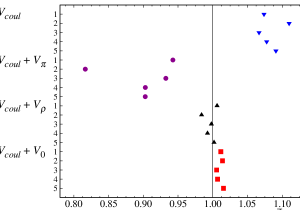
Figure 3: (Color online) Average Coulomb strength parameter, $\overline{\lambda}_{coul}$, as obtained from the fit with the USD interaction to the Range I data selection (see Section III.1 for details). Down (blue) triangles correspond to the fit with Coulomb force alone. The $\overline{\lambda}_{coul}$ obtained from $V_{coul}$ and $V_{\pi}$ are depicted by (purple) dots, and up (black) triangles are $\overline{\lambda}_{coul}$ obtained from $V_{coul}$ and $V_{\rho}$ combination, whereas (red) squares represent $\overline{\lambda}_{coul}$ from a fit with the $V_{coul}$ and $V_{0}$ combination of the two-body charge-dependent forces. Y-axis tic labels: 1, “without SRC”; 2, Miller-Spencer; 3, CD-Bonn; 4, AV-18; 5, UCOM.

We confirm also the conclusion of Ref. Ormand and Brown (1989a) that a combination of the pion and $\rho$ meson exchange potential to model nuclear charge-dependent forces does not allow one to improve the value of the rms deviation. This is why we present here strength parameters only for two combinations of the charge-dependent forces from the list above, namely, (iii) $V_{coul}$ and $V_{\rho}$ and (iv) $V_{coul}$ and $V_{0}$. The resulting rms deviation of these fits and the corresponding Coulomb strengths are indeed rather close, in agreement with the conclusion of Ref. Ormand and Brown (1989a). We discuss both cases in the next section.

Table 5: Various combinations of INC potential and their strength parameters.

Data Range	USD		USDA		USDB
	$V_{coul}+V_{0}$	$V_{coul}+V_{\rho}$	$V_{coul}+V_{0}$	$V_{coul}+V_{\rho}$	$V_{coul}+V_{0}$	$V_{coul}+V_{\rho}$
Range I
rms (keV):
$b$ coefficients	$\scriptstyle\mathtt{\sim}$32.2	$\scriptstyle\mathtt{\sim}$32.7	$\scriptstyle\mathtt{\sim}$35.2	$\scriptstyle\mathtt{\sim}$34.5	$\scriptstyle\mathtt{\sim}$34.3	$\scriptstyle\mathtt{\sim}$33.9
$c$ coefficients	$\scriptstyle\mathtt{\sim}$9.1	$\scriptstyle\mathtt{\sim}$10.5	$\scriptstyle\mathtt{\sim}$10.3	$\scriptstyle\mathtt{\sim}$10.9	$\scriptstyle\mathtt{\sim}$9.7	$\scriptstyle\mathtt{\sim}$10.6
$\overline{\lambda}_{coul}$	1.006 – 1.015	1.002 – 0.9839	1.007 – 1.016	0.9993 – 0.9852	1.008 – 1.018	0.9987 – 0.9845
$-\lambda^{(1)}_{0}\times 100$	0.8162 – 1.637	—	0.7845 – 1.715	—	0.9211 – 1.815	—
$-\lambda^{(2)}_{0}\times 100$	2.629 – 3.861	—	2.915 – 4.227	—	2.851 – 4.122	—
$-\lambda^{(1)}_{\rho}$ (MeV)	—	4.465 – 100.0	—	0.8517 – 82.69	—	2.228 – 89.52
$\lambda^{(2)}_{\rho}$ (MeV)	—	33.52 – 209.8	—	35.27 – 217.1	—	35.40 – 216.9
$\varepsilon^{(1)}_{0d5/2}$ (MeV)	3.278 – 3.279	3.294 – 3.295	3.269 – 3.276	3.295 – 3.298	3.267 – 3.272	3.293 – 3.295
$\varepsilon^{(1)}_{0d3/2}$ (MeV)	3.277 – 3.299	3.294 – 3.302	3.273 – 3.298	3.301 – 3.312	3.265 – 3.286	3.297 – 3.306
$\varepsilon^{(1)}_{0s1/2}$ (MeV)	3.319 – 3.336	3.344 – 3.346	3.327 – 3.346	3.360 – 3.367	3.323 – 3.341	3.358 – 3.362
Range II
rms (keV):
$b$ coefficients	$\scriptstyle\mathtt{\sim}$44.1	$\scriptstyle\mathtt{\sim}$44.1	$\scriptstyle\mathtt{\sim}$46.4	$\scriptstyle\mathtt{\sim}$47.0	$\scriptstyle\mathtt{\sim}$45.5	$\scriptstyle\mathtt{\sim}$46.6
$c$ coefficients	$\scriptstyle\mathtt{\sim}$9.3	$\scriptstyle\mathtt{\sim}$10.6	$\scriptstyle\mathtt{\sim}$10.4	$\scriptstyle\mathtt{\sim}$10.9	$\scriptstyle\mathtt{\sim}$9.8	$\scriptstyle\mathtt{\sim}$10.7
$\overline{\lambda}_{coul}$	1.008 – 1.017	0.9808 – 1.005	1.008 – 1.017	0.9826 – 1.006	1.009 – 1.019	0.9814 – 1.005
$-\lambda^{(1)}_{0}\times 100$	1.202 – 2.019	—	1.149 – 2.079	—	1.324 – 2.215	—
$-\lambda^{(2)}_{0}\times 100$	2.611 – 3.843	—	2.901 – 4.213	—	2.836 – 4.106	—
$-\lambda^{(1)}_{\rho}$ (MeV)	—	10.44 – 120.3	—	6.601 – 103.3	—	8.366 – 110.8
$\lambda^{(2)}_{\rho}$ (MeV)	—	33.87 – 212.2	—	35.54 – 219.1	—	35.76 – 219.3
$\varepsilon^{(1)}_{0d5/2}$ (MeV)	3.271 – 3.273	3.289 – 3.291	3.267 – 3.271	3.292 – 3.295	3.257 – 3.261	3.261 – 3.265
$\varepsilon^{(1)}_{0d3/2}$ (MeV)	3.273 – 3.295	3.283 – 3.290	3.271 – 3.296	3.289 – 3.299	3.266 – 3.288	3.262 – 3.282
$\varepsilon^{(1)}_{0s1/2}$ (MeV)	3.283 – 3.301	3.300 – 3.304	3.290 – 3.310	3.313 – 3.322	3.320 – 3.342	3.286 – 3.305
Range III
rms (keV):
$b$ coefficients	$\scriptstyle\mathtt{\sim}$65.0	$\scriptstyle\mathtt{\sim}$65.2	$\scriptstyle\mathtt{\sim}$67.4	$\scriptstyle\mathtt{\sim}$67.4	$\scriptstyle\mathtt{\sim}$65.7	$\scriptstyle\mathtt{\sim}$66.0
$c$ coefficients	$\scriptstyle\mathtt{\sim}$10.2	$\scriptstyle\mathtt{\sim}$10.5	$\scriptstyle\mathtt{\sim}$11.3	$\scriptstyle\mathtt{\sim}$10.8	$\scriptstyle\mathtt{\sim}$10.6	$\scriptstyle\mathtt{\sim}$10.5
$\overline{\lambda}_{coul}$	1.015 – 1.025	0.9743 - 1.004	1.017 – 1.027	0.9780 – 1.007	1.018 – 1.028	0.9752 – 1.005
$-\lambda^{(1)}_{0}\times 100$	2.331 – 3.189	—	2.453 – 3.423	—	2.591 – 3.515	—
$-\lambda^{(2)}_{0}\times 100$	2.408 – 3.648	—	2.690 – 4.012	—	2.634 – 3.915	—
$-\lambda^{(1)}_{\rho}$ (MeV)	—	37.85 – 228.6	—	3.300 – 210.6	—	36.02 – 220.4
$\lambda^{(2)}_{\rho}$ (MeV)	—	33.61 – 215.0	—	35.04 – 221.1	—	35.54 – 222.5
$\varepsilon^{(1)}_{0d5/2}$ (MeV)	3.245 – 3.247	3.256 – 3.258	3.237 – 3.241	3.261 – 3.262	3.233 – 3.237	3.260 – 3.261
$\varepsilon^{(1)}_{0d3/2}$ (MeV)	3.228 – 3.251	3.169 – 3.186	3.226 – 3.251	3.179 – 3.191	3.219 – 3.240	3.174 – 3.187
$\varepsilon^{(1)}_{0s1/2}$ (MeV)	3.152 – 3.168	3.125 – 3.127	3.147 – 3.165	3.125 – 3.127	3.153 – 3.170	3.127 – 3.131

III.3.2 rms Deviation Values and Strength Parameters

Table 5 gives an overview of strength parameters for two types of the INC Hamiltonian: (iii) $V_{coul}$ and $V_{\rho}$ (columns 3, 5, and 7) and (iv) $V_{coul}$ and $V_{0}$ (columns 2, 4, and 6). Calculations have been performed with the USD, USDA, and USDB nuclear Hamiltonians and for each of the three data ranges. All four approaches to SRC (Jastrow type function with three different parametrizations or UCOM) from Section II.2.2 have been tested and the intervals of parameter variations are indicated in the table.

As seen from Table 5, the rms deviation changes little for various types of the SRC (within 1 keV) and for both types of the charge-dependent Hamiltonian.

The rms deviation turns out to depend mainly on the number of data points used in a fit. It is remarkable that although Range I   contains almost twice the number of data points of Ref. Ormand and Brown (1989a), the rms deviation increases only by $\scriptstyle\mathtt{\sim}$5 keV. Overall, the rms deviation of Range II  is $\scriptstyle\mathtt{\sim}$30% higher compared to Range I, while the rms deviation value for Range III   is about twice as large as that of Range I. It should also be remembered that low-lying states calculated with the isospin-conserving USD/USDA/USDB interactions are in general in better agreement with experiment than high-lying states.

We notice that the USD interaction always produces slightly lower rms deviations than USDB and USDA. This happens even in the fits to Range III   data, although the USD was adjusted to a smaller set of excited levels as compared to the later versions USDA and USDB.

Variations in the values of the parameters indicated in each entry of the table are due to the different SRC approaches. In general, more quenched expectation value of an operator results in a higher value of the corresponding parameter strength. The most crucial role is played by the Coulomb potential, since it is the major contribution to isobaric mass splittings. Deviations can be slightly greater or less than unity for different combinations of charge-dependent forces.

To reduce the discrepancy, the strengths of the charge-dependent forces of nuclear origin, $\lambda_{\nu\neq coul}^{(q)}$, are adjusted in the fit in a way to match experimental isobaric mass splittings. We keep the isovector and isotensor strengths of the nuclear charge-dependent forces as two independent parameters.

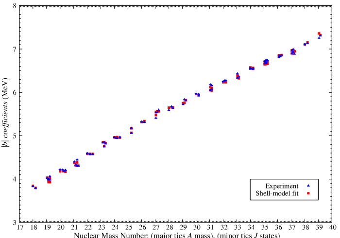
Figure 4: (Color online) Experimental and theoretical $|b|$ coefficients in $sd$-shell nuclei plotted as a function of $A$. Minor $x$-axis tics are $J$ states, which are arranged in an increment of 0.05 for every $\frac{1}{2}$ step.

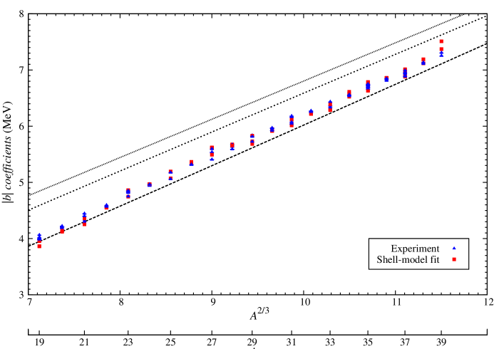
Figure 5: (Color online) Experimental and theoretical $|b|$ coefficients in $sd$-shell nuclei plotted as a function of $A^{2/3}$. Dot-dashed line is $|b|=\frac{3e^{2}(A-1)}{5r_{0}A^{1/3}}$, double-dot-dashed line is $|b|=\frac{3e^{2}}{5r_{0}}A^{2/3}$, the dashed line represent $b$ values from Möller and Nix model Eq. (29).

$V_{coul}$ and $V_{0}$ combination.

These combinations almost always produce the lowest rms deviations for $b$ and $c$ coefficients. Fitted to the smallest range of data, the isovector and isotensor strengths of the nuclear isospin-violating contribution represent about 0.7–1.7% and 2.9 – 4.2%, respectively, of the original isospin-conserving $sd$ interaction. We notice that in a fit to the Range III data, the charge-asymmetric part of the interaction increases up to 2.3–3.2% of the nuclear interaction.

The Miller-Spencer parametrization and UCOM SRC schemes quench the Coulomb expectation values more than the AV-18 and CD-Bonn parametrizations (see Table 2 as an example). This is why the highest values of $\overline{\lambda}_{coul}$ in columns 2, 4, and 6 belong to UCOM SRC and $\overline{\lambda}_{coul}$ of the Miller-Spencer parametrization SRC are very close to them. At the same time, those parametrizations result in the most negative values of $\lambda_{0}^{(q)}$ in columns 2, 4, and 6 to compensate for the Coulomb effect.

$V_{coul}$ and $V_{\rho}$ combination.

For the combination of the Coulomb and Yukawa $\rho$-exchange type potentials as the isospin-symmetry breaking forces it should be noted that typical expectation values of $V_{\rho}$ are about 3 to 4 orders of magnitude smaller than the expectation values of $V_{coul}$. Therefore, small variations in the Coulomb strength (of the order of 1-2%) require a factor of up to 20 variation in the corresponding strength $\lambda_{\rho}^{(q)}$ (e.g., the magnitudes of isovector $\rho$-exchange strengths range from 4.4 to 100 for the USD interaction in the Range I data selection). So, the $\rho$-exchange potential strength is very sensitive to the SRC procedure. It is not surprising that the lowest absolute $\lambda_{\rho}^{(q)}$ in columns 3, 5, and 7, corresponds to evaluations without taking SRC into account; however, with the presence of SRC, the lowest absolute $\lambda_{\rho}^{(q)}$ are from the CD-Bonn parametrization. The lowest $\overline{\lambda}_{coul}$ and, therefore, the highest absolute $\lambda_{\rho}^{(q)}$ in columns 3, 5, and 7 belong to the Miller-Spencer parametrization SRC. The $\overline{\lambda}_{coul}$ values being closest to unity are from the CD-Bonn and UCOM SRC schemes for the three ranges of data (see also Fig. 3).

Again we notice an increase of the isovector parameter $\lambda_{\rho}^{(1)}$ in a fit to the Range III data. It was mentioned in Ref. Ormand and Brown (1989a), at that time it was not possible to conclude in that work whether the small asymmetry of the effective interaction is due to the original asymmetry of a bare NN force, or whether it was a radial wave function effect Lawson (1979). Our present results show that including more and more excited states lead to a bigger asymmetry value. Most probably, it is due to the radial wave functions effect, since asymmetry in the proton and neutron wave functions becomes larger in higher excited states.

Regarding the ISPE’s, their values stay consistent within certain intervals. Amazingly, the value of $\varepsilon^{(1)}_{0d5/2}$ stays almost constant, without showing any dependence on the particular SRC approach, most probably, because it is the orbital which is most constrained by the data. At the same time, the value of $\varepsilon^{(1)}_{0d3/2}$ depends somewhat on the SRC procedure. The highest value of $\varepsilon^{(1)}_{0d3/2}$ in column 2 always corresponds to the Miller-Spencer parametrization SRC. The values of $\varepsilon^{(1)}_{0d3/2}$ and $\varepsilon^{(1)}_{1s1/2}$ change much less for the $V_{coul}$ and $V_{\rho}$ combination, than for the $V_{coul}$ and $V_{0}$ combination (with the exception of the USDB interaction in the Range II data fit). As a general trend we notice a reduction of the values of ISPE’s when we increase the number of data points in a fit.

The values of parameters given in Table 5 lie outside the intervals obtained by Ormand and Brown who considered the $V_{coul}$ and $V_{0}$ combination. In particular, we get systematically lower values of the isotensor strength parameter $\lambda_{0}^{(2)}$, as well as lower values of $\varepsilon^{(1)}_{0d5/2}$, even for the Range I of data.

The inclusion of nuclei from the middle of the $sd$ shell, combined with the latest experimental data and with the newly developed approaches to SRC allowed us to construct a set of high-precision isospin-violating Hamiltonians in the full $sd$ shell-model space. They reproduce the experimental $b$ and $c$ coefficients with very low rms deviations, c.f. Table 5. The ratios of the rms deviations of various SRCs, with USD, USDA, and USDB to the average $|b|$ coefficients in $sd$-shell space are less than $\scriptstyle\mathtt{\sim}$0.01. A few applications of these Hamiltonians are considered in the next sections.

IV Theoretically Fitted $b$ and $c$ Coefficients

Theoretical $b$ and $c$ coefficients discussed in this section are obtained in a fit of the parameters of the charge-dependent Hamiltonian, consisting of the Coulomb interaction (with UCOM type of the SRC) and $V_{0}$, on top of the USD interaction, to the experimental data from Range I. The obtained numerical values, as well as corresponding experimental data, are given in Tables  12–15 for doublets, triplets, quartets, and quintetes, respectively.

Before we begin the discussion, let us consider predictions for $b$ and $c$ coefficients given by the uniformly-charged sphere model Bethe and Bacher (1936). In this approach, the total Coulomb energy of a nucleus is considered as a uniformly charged sphere of radius $R=r_{0}A^{1/3}$,

$$E_{coul} =\frac{3e^{2}}{5R}Z(Z-1)$$ (24)

$$=\frac{3e^{2}}{5r_{0}A^{\frac{1}{3}}}\left[\frac{A}{4}(A-2)+(1-A)T_{z}+T_{z}^{2}\right]\,,$$

giving rise to the following expressions for $b$ and $c$ coefficients of the IMME  Bentley and Lenzi (2007); Benenson and Kashy (1979):

$$b =-\frac{3e^{2}}{5r_{0}}\frac{(A-1)}{A^{\frac{1}{3}}}\,,$$

$$c =\frac{3e^{2}}{5r_{0}}\frac{1}{A^{\frac{1}{3}}}\,,$$ (25)

where $e^{2}=1.44$ MeV$\cdot$fm and we use here the value of $r_{0}=1.27$ fm.

Assuming $Z(Z-1)\approx Z^{2}$ in Eq. (24), one can get an even simpler form of $b$ coefficients, namely,

$$b=-\frac{3e^{2}}{5r_{0}}A^{2/3}\,.$$ (26)

A much more precise estimation of $b$ coefficients can be obtained from from the Coulomb energy containing in the the macroscopic part of Möller and Nix model Möller and Nix (1988), namely,

$$E_{Coul}(A,Z) =c_{1}\frac{Z^{2}}{A^{1/3}}B_{3}-c_{4}\frac{Z^{4/3}}{A^{1/3}}$$

$$+f(k_{f}r_{p})\frac{Z^{2}}{A^{1/3}}-c_{a}(N-Z)\,,$$ (27)

where $c_{1}=3e^{2}/(5r_{0})$ and $c_{4}=5/4(3/(2\pi))^{2/3}c_{1}$ are parameters entering in the direct and exchange Coulomb energy terms, respectively, the proton form-factor correction (the third term) estimated for the nuclei in the middle of $sd$ shell ($Z=14$, $A=28$) and the proton radius $r_{p}=0.8$ fm involves $f=-0.2138$ MeV, while the charge-asymmetry term (the last term) enters with $c_{a}=0.145$ MeV. The parameter $B_{3}$ defining in general the relative Coulomb energy for an arbitrary shape nucleus has in the leading order (for a spherical nucleus) the following expression:

$$B_{3}=1-\frac{5}{y_{0}^{2}}+\frac{75}{8y_{0}^{3}}-\frac{105}{8y_{0}^{5}}$$ (28)

with $y_{0}=\alpha A^{1/3}$, and $\alpha=r_{0}/a_{den}\approx 1.657$.

From Eq. (IV), one can get the following expression for the IMME $b$ and $c$ coefficients:

$$b = c_{1}A^{2/3}+\frac{75c_{1}}{8\alpha^{3}}A^{-1/3}-\frac{105c_{1}}{8\alpha^{5}}A^{-1}\,$$ (29)

$$- \frac{5c_{1}}{\alpha^{2}}-\frac{4c_{4}}{3(2)^{1/3}}+f(k_{f}r_{p})+2c_{a}\,,$$

$$c = c_{1}A^{-1/3}-\left(\frac{5c_{1}}{\alpha^{2}}+\frac{4c_{4}}{9(2)^{1/3}}\right)A^{-1}\,$$ (30)

$$+ f(k_{f}r_{p})A^{-1}+\frac{75c_{1}}{8\alpha^{3}}A^{-4/3}-\frac{105c_{1}}{8\alpha^{5}}A^{-2}\,,$$

which lead to the following numerical expressions:

$$b = 0.7448A^{2/3}-1.8819+1.535A^{-1/3}\,$$ (31)

$$- 0.7826A^{-1}\,[\textnormal{MeV}]\,,$$

$$c = 0.7448A^{-1/3}-1.771A^{-1}+1.535A^{-4/3}\,$$ (32)

$$- 0.7826A^{-2}\,[\textnormal{MeV}]\,.$$

We will use these estimations in our analysis of the values obtained by a shell-model fit.

IV.1 Fitted $b$ Coefficients

Theoretical $b$ coefficients are shown in Figs. 4 and 5 in comparison with experimentally deduced values Lam et al. (bles). Overall, the deviations of $b$ coefficients obtained in a shell-model fit from the experimental ones are less at the top and the bottom of $sd$-shell space than the deviations in the middle shell. The only exception is the $\frac{1}{2}^{+}$ doublet of $A=39$ for which the difference between theoretical and experimental $b$ coefficients comes out to be 107.6 keV. However, if we refit the Hamiltonian parameters according to the smaller data range selected in Ref. Ormand and Brown (1989a) (the bottom and the top of the $sd$ shell), this deviation for the $\frac{1}{2}^{+}$ doublet of $A=39$ reduces to 49.8 keV. Thus the reason for a noticeable discrepancy for that point in a full $sd$ shell Range I fit may be due to the inclusion of data from the middle shell. On the other hand, if we refit the parameters using extended data sets, Range II and Range III, this deviation reduces to 82 keV and to 0.7 keV, respectively. It is because the addition of more data points renormalizes the discrepancies of the fit. Although the inclusion of the $b$ coefficient of the $\frac{1}{2}^{+}$ doublet of $A=39$ reduces the quality of the fit, we retain it in the data set to adjust the ISPEs $\varepsilon^{(1)}_{i}$ in Eq. (II.1).

Let us remark that the quality of the fit is already somewhat pre-determined by the quality of the original isospin-conserving two-body interaction. For example, a very accurate description of low-lying states in $A=35$ nuclei by the USD interaction leads to the values of theoretical $b$ coefficients of the $A=35$ doublets which are close to the experimental ones (see Table  12). Another factor, the major factor, that influences the values of the obtained deviations is a characteristic property of the error-weighted least-squares fit. Experimental $b$ coefficients with very low error bars are favored in the shell-model fit and the corresponding theoretical $b$ coefficients have typically rather low deviations. This is the reason why most of the lowest-lying multiplets’ $b$ coefficients are very close to experimental values. For example, the deviation between theoretical and experimental $b$ coefficients of the mass $A=32$ quintet, the best known quintet in the $sd$ shell, is the lowest among the five quintets. Therefore, advances in mass measurements and nuclear excitation energies providing data points with low error bars may influence the data, which are dominant in adjusting the strengths of charge-dependent forces in the INC Hamiltonian; in particular, data from the top and from the bottom of $sd$-shell space, which are used to calibrate the ISPEs. Similar magnitudes of deviations are obtained for other combinations of charge-dependent forces. For the USDA and USDB interactions (with either $V_{coul}+V_{0}$ or $V_{coul}+V_{\rho}$, and with different SRC schemes), the deviations are a few keV higher than those obtained in the calculations with the USD interaction.

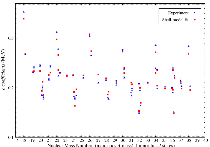
Figure 6: (Color online) Experimental and theoretical $c$ coefficients plotted as a function of $A$. Minor $x$-axis tics are $J$ states, which are arranged in an increment of 0.05 for every $\frac{1}{2}$ step.

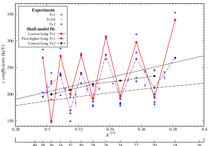
Figure 7: (Color online) Experimental and theoretical $c$ coefficients in $sd$-shell nuclei plotted as a function of $A^{-1/3}$. The black dashed line represents $c$ coefficients from a charged sphere model, while the double-dot-dashed line shows the prediction according to Möller and Nix model Eq. (30).

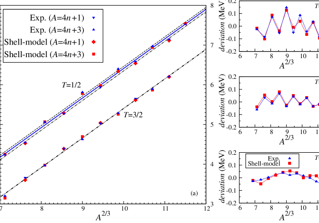
Figure 8: (Color online) Staggering effect of the $b$ coefficients of the ground-state doublets and of the lowest-lying quartets in $sd$-shell nuclei. Plot (a): $|b|$ values of the ground-state doublets (left $y$ axis) and the lowest-lying quartets (right $y$-axis). For $T=1/2$, the solid (blue) line $b=0.7447A^{2/3}-1.2551$ (MeV), the dashed (black) line $0.7442A^{2/3}-1.1987$, and the dot-dashed (black) line $b=0.7463A^{2/3}-1.3329$ (MeV), represent best fits to experimental values for the all $A$, $A=4n+3$ and $A=4n+1$ isobars, respectively. For $T=3/2$, the double-dot-dashed line $b=0.7441A^{2/3}-1.2547$ (MeV) is obtained by a fit to all experimental $b$ coefficients. Plots (b) – (d): deviations of $b$ coefficients from the respective fitted to all data points lines. The experimental $b$ values are represented by (blue) triangles and $b$ obtained in a shell-model fit are shown by (red) squares.

As suggested by Eq. (26), we plot experimental and theoretical $b$ coefficients (obtained from a shell model fit) as a function of $A^{2/3}$ in Fig. 5. It is evident that theoretical values are in remarkable agreement with the experimental data. For comparison, we show $b$ coefficients obtained from the uniformly charged sphere model and from the Möller and Nix model as well. Predictions of the former reproduce well the trend of the $b$ coefficients, however, they are about 500 keV off the experimental values when given by Eq. (IV) and there is even a larger discrepancy (about 800 keV) for a simplified form given by Eq. (26). Clearly, the ratio $1/Z$ for $sd$-shell space nuclei is not negligible with respect to $Z$. The Möller and Nix model produces a much better agreement with the experimental data, slightly underestimating the experimental values on average.

Although it is not seen in the scale of Fig. 5, in fact, the $b$ coefficients in the $sd$ shell-model space exhibit some regular oscillations around a straight line, representing the best fit of a linear function of $A^{2/3}$ to the data points. This effect is discussed in Section  IV.3.

IV.2 Fitted $c$ Coefficients

The $c$ coefficients obtained in the shell-model fit (see Tables  13 – 15) are plotted in Figs. 6 and 7. The discrepancy between theoretical and experimental values for nuclei from the top and from the bottom of $sd$ shell-model space are larger than for nuclei from the middle of the shell. Possible reasons for this have been mentioned above, namely, it can be due to the larger experimental error bars and/or lower accuracy of the corresponding isospin-conserving Hamiltonian to describe the energy levels. In Fig. 7, we plot the $c$ coefficients as a function of $A^{-1/3}$ as suggested by Eq. (IV). Let us remark a few interesting features:

• One easily notices a well pronounced oscillatory trend in the lowest-lying triplets’ $c$ coefficients connected by the solid line in Fig. 7. These values are always the highest or the lowest $c$ coefficients, except for $A=20,24,28$, and $32$. This trend is also inherent to the corresponding experimental $c$ coefficients Lam et al. (bles).

• The first higher-lying triplets’ $c$ coefficients also exhibit regular oscillations, but of a smaller amplitude than those described above. The corresponding shell-model data points are connected by a double-dot-dashed line.

• The other higher-lying triplets’ and quartets’ $c$ coefficients lie somewhere in the middle part of the plot between maxima and minima of low-lying triplets’ $c$ coefficients without any particular behavior. The quartets’ $c$ coefficients do not display any staggering effect. The quintets’ $c$ coefficients connected by the dot-dashed line follow well the prediction of the uniformly charged sphere, $c=\frac{3e^{2}}{5r_{0}}A^{-1/3}$ (dashed line).

The shell-model $c$ coefficients are seen to be in very good agreement with the experimental data. The uniformly charged sphere model describes well the overall trend of $c$ coefficients, following about the average values, but it cannot predict the oscillatory behavior of the $c$ coefficients. Similarly, the $c$ coefficients from Möller and Nix model exhibit quite a smooth trend, reproducing well the experimental values for $A=4n$ multiplets.

IV.3 Staggering Behavior of $b$ and $c$ Coefficients

The oscillatory effects in IMME $b$ and $c$ coefficients were noticed by Jänecke in the 1960’s, c.f. Refs. Jänecke (1969, 1966), although at that moment the available experimental data was limited to $T\leq 1$ multiplets. Since then, a few analytical models have been proposed to explain the oscillatory effect. One of the approaches, proposed by Hecht Hecht (1968), was based on Wigner’s supermultiplet scheme. Another explanation was given by Jänecke  Jänecke (1969, 1966) in the framework of a schematic approach to Coulomb pairing effects.

In this section we revisit the staggering effect of the $b$ and $c$ coefficients of $sd$-shell nuclei based on a much more extended set of experimental data, which fully covers the lowest-lying doublets, triplets, quartets, and quintets, and we explore it theoretically using the constructed empirical INC shell-model Hamiltonian. For the first time, we identify contributions of various isospin-symmetry breaking terms to $b$ coefficient (isovector energy) and $c$ coefficient (isotensor energy).

IV.3.1 Perspective of Empirical INC Hamiltonians

To evidence a staggering phenomenon, we plot the $b$ coefficients obtained from experiment and from a shell-model fit for the lowest-lying doublets and quartets in $sd$-shell nuclei in Fig. 8(a). The oscillatory behavior of the $b$ coefficients of doublets and quartets is clearly seen now. The data points form two families for $A~{}=~{}4n~{}+~{}1$ and $A~{}=~{}4n~{}+~{}3$ multiplets lying slightly above and under the middle straight line, respectively. There is no staggering effect in the $b$ coefficients of $T=1$ triplets, c.f. Fig. 8 (d). This general behavior of the $b$ coefficients of doublets, quartets and triplets agree with what had been noticed by Jänecke  Jänecke (1966) and by Hecht Hecht (1968). The quintets’ $b$ coefficients are known only for the lowest $A~{}=~{}4n$ multiplets and therefore we cannot discuss them on the same footing due to missing data.

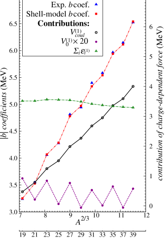
Figure 9: (Color online) Contributions of the various charge-dependent forces to doublet ($T=1/2$) $b$ coefficients. The $|b|$ values are plotted as a function of $A^{2/3}$. The total $|b|$ values refer to the left $y$-axis, while contributions from $V_{coul}^{(1)}$, from $V_{0}^{(1)}$, and from the summed ISPE $\sum_{i}\epsilon_{i}^{(1)}$, refer to the right $y$-axis. The contribution from $V^{(1)}_{0}$ is multiplied by 20.

Figure 10: (Color online) Contributions of the various charge-dependent forces to the lowest-lying quartet ($T=3/2$) $b$ coefficients. Refer to Fig. 9 for further description.

To magnify the effect of oscillations, we show deviations of the experimental and theoretical values from fitted middle lines (solid line for $T=1/2$ multiplets and double-dot-dashed line for $T=3/2$ multiplets) in Fig. 8(b) and Fig. 8(c). Interestingly, the oscillations of doublet $b$ coefficients are of a higher amplitude compared to those of quartet $b$ coefficients and they are in opposite direction. This tendency is naturally manifested in Wigner’s supermultiplet theory Jänecke (1969); Lam (2011); Van Isacker et al. (tion). As seen from these figures, the $b$ coefficients obtained in a shell-model fit for doublets and quartets follow the experimental trend extremely accurately, reproducing very precisely the general trend and the staggering amplitude.

Since, the charge-dependent term in the INC Hamiltonian is given by a combination of three components, $\lambda_{coul}V_{coul}$, $\lambda_{0}V_{0}$ and ISPEs, $\sum_{i}\epsilon_{i}$, we can explore what contribution from each component to the total $b$ value is. The results are shown in Fig. 9 and Fig. 10 for the doublets’ and the quartets’ $b$ coefficients, respectively.

Qualitative analysis leads to rather similar conclusions for both doublets’ and quartets’ $b$ coefficients. The isovector Coulomb component is the main contribution to the staggering effects of the $b$ coefficients of doublets and quartets (Figs. 9 and 10, respectively). It is interesting to note that the isovector charge-dependent term of nuclear origin, $\lambda_{0}V_{0}^{(1)}$, produces the same oscillatory trend as that from the Coulomb force, but of a much smaller amplitude. The one-body contribution, however, does not produce any oscillations. This could be expected, since the staggering effect is due to the manifestation of the Coulomb contribution to the pairing.

In general, the values of higher-lying multiplets’ $b$ coefficients follow more and more smooth trends and the staggering gradually disappears.

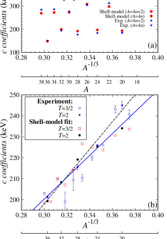
Figure 11: (Color online) Staggering effects of $c$ coefficients of the lowest-lying triplets (plot (a)), and quartets and quintets (plot (b)). See text for discussion. In the lower panel, the dot-dashed (black) line, $c=651.6A^{-{1/3}}+2.6$ (keV), is an unweighted fit to the experimental $c$ coefficients. The solid (blue) line, $c=520.7A^{-{1/3}}+44.1$ (keV), is an unweighted fit to the $c$ coefficients obtained in a shell-model fit.

The general features of staggering have already been discussed in section IV.2. In Fig. 11 we plot separately the $c$ coefficients of the lowest-lying triplets (the upper part of the figure) and the lowest-lying quartets and quintets (the lower part of the figure) in $sd$-shell nuclei. The $c$ coefficients obtained in the shell-model fit reproduce the experimental values very precisely (with the largest deviation of about 15 keV, see also Tables 13 – 15).

The experimental and shell model fitted $c$ coefficients of triplets clearly form two distinct families of multiplets for $A=4n$ and $A=4n+2$ nuclei, respectively. However, no oscillations can be noticed for $T=3/2$ multiplets. The $c$ coefficients of quintets are known only for $A=4n$ multiplets which follow a quite smooth trend with mass number.

Contributions of different terms of the charge-dependent Hamiltonian to the lowest-lying triplets’ $c$ coefficients are shown in Fig. 12. One can see that the isotensor Coulomb force $V_{coul}^{(2)}$ plays the major role. Furthermore, the plot also indicates that $V_{coul}^{(2)}$ alone does not reproduce the magnitude of the experimental $c$ coefficients. For the $A=4n+2$ family, the deviation is about $\scriptstyle\mathtt{\sim}$40 keV, while for the $A=4n$ family, it is around $\scriptstyle\mathtt{\sim}$5 keV. This indicates that the Coulomb interaction should be supplemented by another two-body interaction of nuclear origin, which we model as $V_{0}^{(2)}$ (or $V_{\rho}^{(2)}$) in this paper and which perfectly fulfills its task. The contribution of the empirical isotensor nuclear interaction results in the same oscillatory trend as that of the isotensor Coulomb component, with the values being of about $\scriptstyle\mathtt{\sim}$40 keV for $A=4n$ multiplets and $\scriptstyle\mathtt{\sim}$5 keV for $A=4n+2$ multiplets (with a negative value for the lowest $A=36$ triplet). Thus, the experimental values of $c$ coefficients are perfectly reproduced.

A similar decomposition of the theoretical $c$ coefficients for quintets is given in Fig. 13. As has been already mentioned, the data on $A=4n+2$ multiplets is required in order to establish the existence of the staggering effect. It is seen, however, that the contribution from the isotensor nuclear force to quintets’ $c$ coefficients shows some noticeable oscillatory effect between $A=8n$ and $A=8n+4$ multiplets. It may possibly change to the staggering characteristics for triplets’ $c$ coefficients when data on $A=4n+2$ becomes available.

The $c$ coefficients of high-lying multiplets are systematically known only for triplets. As it was mentioned in the previous section, the first high-lying triplets’ $c$ coefficients oscillate with a smaller amplitude, while $c$ coefficients of other high-lying multiplets follow a more or less smooth trend. This is probably related to the destroying of the pairing effects with increasing excitation energy in nuclear systems.

Very similar trends and exactly the same conclusions can be inferred if other $sd$-shell model interactions are used instead of USD, or other charge-dependent Hamiltonians (with other SRC schemes). This proves the robustness of the effects described above.

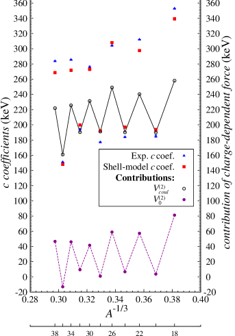
Figure 12: (Color online) Contributions of the various charge-dependent forces to the lowest-lying triplet $c$ coefficients. All $c$ values refer to the left $y$-axis, while the contributions from $V_{coul}^{(2)}$, and $V_{0}^{(2)}$ refer to the right $y$-axis.

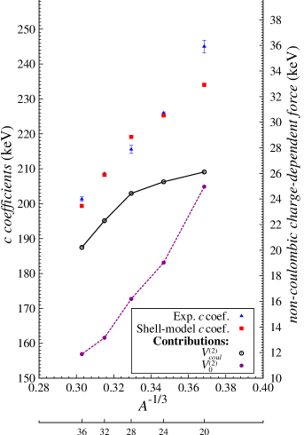
Figure 13: (Color online) Contributions of the various charge-dependent forces to the lowest-lying quintet $c$ coefficients. All $c$ values and the contribution from $V_{coul}^{(2)}$ refer to the left $y$-axis, while the contribution from $V_{0}^{(2)}$ refer to the right $y$-axis.

IV.3.2 Jänecke’s Schematic Model

Jänecke’s model Jänecke (1966, 1969) is based on an approximate formula for the Coulomb energy of valence proton(s) outside a closed shell, which was proposed by Carlson and Talmi Carlson and Talmi (1954). In order to match the trend of the total Coulomb energy of a nucleus as represented by the IMME, Jänecke replaced the Coulomb pairing term Carlson and Talmi (1954) by a quadratic term in $T_{z}$  Jänecke (1966). As a result, one can deduce the following expressions for isovector, $E_{coul}^{(1)}$, and isotensor, $E_{coul}^{(2)}$, contributions,

$$E_{coul}^{(1)}=\frac{1}{2}E_{1}A+E_{2}+\mu E_{3}\,,$$ (33)

and

$$E_{coul}^{(2)}=\frac{1}{6}\left(E_{1}+2\nu E_{3}\right)\,,$$ (34)

where the energies $E_{i}$ are related to one and two-body electromagnetic interactions, while $\mu$ and $\nu$ are some parameters. In Ref. Jänecke (1966), assuming an independent-particle model with four-fold degenerate orbitals, Jänecke could estimate a probability for the number of proton pairs to occupy the same orbital and, thus, he could deduce a contribution to the Coulomb energy for a given $A$ and $T$. He obtained the following parametrization for $\mu$ and $\nu$ values:

$$\mu=\left\{\begin{array}[]{ll}\displaystyle\frac{1}{2}&\quad A\textnormal{-even}\\ \displaystyle\frac{1}{2}\left(1-\frac{(-1)^{A/2-T}}{2T}\right)&\quad A\textnormal{-odd}\end{array}\right.$$ (35)

and

$$\nu=\left\{\begin{array}[]{ll}\displaystyle\frac{1}{4T}\left(1+\frac{(-1)^{A/2-T}}{2T-1}\right)&\quad A\textnormal{-even}\\ \displaystyle\frac{1}{4T}&\quad A\textnormal{-odd},T>\frac{1}{2}\,.\end{array}\right.$$ (36)

As was remarked in Ref. Jänecke (1966), the coefficients $E_{i}$ with $i=1,2,$ and 3, are related to the expectation value of $1/r$, because the average distance between protons should increase with the nuclear volume. Therefore, if we assume that $E_{i}=\hat{E}_{i}/A^{1/3}$, with $\hat{E}_{i}$ being constant values, different from one shell to another shell, the isovector Coulomb energy will become a linear function of $A^{2/3}$ and the isotensor energy will be a linear function of $A^{-1/3}$ (since $E_{1}$ is the leading term in expressions (Eq. (33)–Eq. (34)).

Isovector Coulomb Energies.

Using Eq. (33) and the respective $\mu$ values, we may derive the isovector Coulomb energies for doublets, triplets, quartets and quintets as

$$E_{coul\,(T=1/2)}^{(1)} =\frac{1}{2}E_{1}A+E_{2}+\frac{1}{2}E_{3}+(-1)^{(A+1)/2}\frac{E_{3}}{2}\,,$$ (37)

$$E_{coul\,(T=1)}^{(1)} =\frac{1}{2}E_{1}A+E_{2}+\frac{1}{2}E_{3}\,,$$ (38)

$$E_{coul\,(T=3/2)}^{(1)} =\frac{1}{2}E_{1}A+E_{2}+\frac{1}{2}E_{3}+(-1)^{(A-1)/2}\frac{E_{3}}{6}\,,$$ (39)

$$E_{coul\,(T=2)}^{(1)} =\frac{1}{2}E_{1}A+E_{2}+\frac{1}{2}E_{3}\,,$$ (40)

respectively. From the last terms of Eq. (37) and Eq. (39), determining the amplitude of the oscillations of the $b$ coefficients of doublets and quartets, we see that the amplitude of quartets’ $c$ coefficients is predicted to be three times smaller than that for doublets. Eqs. (38) and (40) indicate that no oscillatory behavior is expected for triplets’ and quintets’ isovector Coulomb energies (or $b$ coefficients).

Isotensor Coulomb Energies.

From Eqs. (34) and (36), we can obtain the isotensor Coulomb energies for triplets, quartets and quintets as

$$E_{coul\,(T=1)}^{(2)} =\frac{1}{6}\left(E_{1}+\frac{1}{2}\left[1-(-1)^{A/2}E_{3}\right]\right)\,,$$ (41)

$$E_{coul\,(T=3/2)}^{(2)} =\frac{1}{6}\left(E_{1}+\frac{1}{3}E_{3}\right)\,,$$ (42)

$$E_{coul\,(T=2)}^{(2)} =\frac{1}{6}\left(E_{1}+\frac{1}{4}\left[1-\frac{1}{3}(-1)^{(A-2)/2}E_{3}\right]\right)\,,$$ (43)

respectively. The last term of Eq. (41) and Eq. (43) shows that triplets’ and quintets’ $c$ coefficients exhibit regular oscillations as a function of $A$, with the amplitude for triplets being six times larger than that for quintets ($c=3E_{coul}^{(2)}$, see Eq. (9)). Eq. (42) shows that the quartets’ isotensor Coulomb energy $E_{coul\,(T=3/2)}^{(2)}$ is predicted to be a constant which may vary from one shell to another. Hence, an oscillatory behavior is not predicted for quartets’ $c$ coefficients.

Performing a linear fit to the experimental $b$ coefficients for the lowest-lying doublets, we have determined the values of $E_{1}=487$ keV, $E_{2}=1199$ keV, and $E_{3}=134$ keV for $sd$-shell nuclei. The value of $E_{3}$ deduced from the fit to $b$ coefficients predicts the $\frac{1}{2}E_{3}=68$ keV amplitude for $c$ coefficients in $T=1$, which is in very good agreement with the experimental value. Analysis of staggering in other model spaces and the values of $E_{i}$ coefficients will be published elsewhere Van Isacker et al. (tion).

V Masses and Extension of the IMME beyond the Quadratic Form. Example of the $A=32$ quintet.

The fit and the analysis in Section  IV.3 are based on the assumption of a quadratic form of the IMME, which is a very good approximation, valid at present for the majority of experimentally measured isobaric multiplets. However, some experimental cases evidence the breaking of the quadratic IMME (e.g., see Refs. Britz et al. (1998); Lam et al. (bles) and references therein, as well as Refs. Triambak et al. (2006); Yazidjian et al. (2007); Kwiatkowski et al. (2009); Kankainen et al. (2010)). We consider here an extended IMME up to a quartic form,

$$M(\alpha,T,T_{z})= a(\alpha,T)+b(\alpha,T)T_{z}+c(\alpha,T)T_{z}^{2}$$ (44)

$$+d(\alpha,T)T_{z}^{3}+e(\alpha,T)T_{z}^{4}\,,$$

with possible non-zero $d$ and/or $e$ coefficients. These higher-order terms in $T_{z}$ can be due to the presence of isospin-symmetry breaking three- (or four-body) interactions among the nucleons Frank et al. (2009), and/or may arise due to the isospin mixing in excited states of isobaric multiplets with nearby state(s) of the same $J^{\pi}$, but different $T$ value. In addition, a special attention should be paid to multiplets of states, involving loosely bound low-$l$ orbitals. Those orbitals in proton-rich members are pushed out of the potential well, which results in smaller values of the Coulomb matrix elements and thus in a smaller Coulomb shifts with respect to their mirrors. This effect known as the Thomas-Ehrman shift Thomas (1952); Ehrman (1951) may also lead to the breaking of the quadratic form of the IMME Benenson and Kashy (1979).

Early theoretical estimations for quartets predicted typical $d$ coefficients to be of the order of $\approx$1 keV Henley and Lacy (1969); Jänecke (1969); Bertsch and Kahana (1970) (see also discussion in Ref. Benenson and Kashy (1979)). To probe such low values, recent experimental advances become crucial in providing precise mass measurements of quartets and quintets. At present, relative mass uncertainties as low as $10^{-8}-10^{-9}$ are reached, see e.g. Refs. Blaum (2006); Kankainen et al. (2010); Triambak et al. (2006); Kwiatkowski et al. (2009).

In the shell model the direct evaluation of absolute binding energies is possible with the isospin-conserving Hamiltonian, provided that a certain algorithm is followed in the subtraction of empirical Coulomb energies from experimental binding energies used in the fit. Then, the subtracted Coulomb energy should simply be added to the shell-model binding energy to get the full theoretical binding energy of a nucleus. In fitting the USD interaction, the subtraction of the Coulomb energy has been done in a kind of average way Warburton et al. (1990); Wildenthal (1984). In particular, an unknown amount of residual isoscalar Coulomb energy may remain in the charge independent nuclear Hamiltonian Warburton et al. (1990); Wildenthal (1984). Adding an INC term in the Hamiltonian requires the precise knowledge of the isoscalar Coulomb contribution and this prohibits the evaluation of absolute binding energies  Ormand (1996). In spite of this fact, we can still well describe theoretical mass differences of isobaric multiplets, which is sufficient to study the $b$, $c$, $d$, and $e$ coefficients of the IMME. The $a$ coefficient, however, remains undetermined. To theoretically explore the validity of the quadratic, cubic or quartic forms of them IMME in a given quintet, we use the results of the exact diagonalization of the INC Hamiltonian, $H_{\textnormal{INC}}$, constructed in the present work. In this way we obtain theoretical mass differences for a given isobaric multiplet and then we fit them with a quadratic, cubic or quartic form of the IMME to find the best $b$, $c$, $d$, and/or $e$ coefficients.

As an example, here we consider in detail the lowest $0^{+}$ quintet in $A=32$.

Table 6: Mass differences and mass summations of $M_{-2}$ and $M_{2}$; and $M_{1}$, $M_{-1}$, and $M_{0}$.

	$M_{-2}-M_{2}$	$M_{1}-M_{-1}$	$M_{1}+M_{-1}-2M_{0}$	$M_{2}+M_{-2}-2M_{0}$
	(keV)	(keV)	(keV)	(keV)
Exp. values	$-21877.48$	$-10944.24$	414.22	1657.26
quoted in Ref. Signoracci and Brown (2011)
Theoretical values
from Ref. Signoracci and Brown (2011):
USD	$-21669.83$	$-10837.25$	418.11	1673.09
USDA	$-21669.62$	$-10836.63$	404.98	1653.43
USDB	$-21672.80$	$-10838.10$	417.25	1667.39
Deduced from Table 15	$-21877.29$	$-10943.63$	413.91	1657.05
Present work:
USD	$-21857.96$	$-10927.87$	414.87	1660.55
USDA	$-21858.35$	$-10927.30$	404.55	1649.76
USDB	$-21858.34$	$-10927.93$	416.24	1664.32

Various experimental determinations of the lowest $T~{}=~{}2$ masses in $A=32$ Kankainen et al. (2010); Triambak et al. (2006); Kwiatkowski et al. (2009) point towards the presence of a non-zero $d$ coefficient in the IMME (see Table 8 later in this section).

Using Eq. (44), we can express the IMME $a,b,c,d$, and $e$ coefficients in terms of the mass excesses of a given $T~{}=~{}2$ quintet,

$$a =M_{0}\,,$$ (45a)

$$b =\frac{1}{12}\left[(M_{-2}-M_{2})+8(M_{1}-M_{-1})\right]\,,$$ (45b)

$$c =\frac{1}{24}\left[16(M_{1}+M_{-1})-(M_{2}+M_{-2})-30M_{0}\right]\,,$$ (45c)

$$d =\frac{1}{12}\left[(M_{2}-M_{-2})+2(M_{1}-M_{-1})\right]\,,$$ (45d)

$$e =\frac{1}{24}\left[-4(M_{1}+M_{-1})+(M_{2}+M_{-2})+6M_{0}\right]\,.$$ (45e)

Here, we have shortened the notation for $a,b,c,d$, and $e$ coefficients and the notation for mass excess of each member ($M_{T_{z}=i}\equiv M_{i}$, $i=-2,-1,0,1,2$). Eqs. (45b) and (45d) show that $b$ and $d$ coefficients are related to the differences $(M_{-2}-M_{2})$ and $(M_{1}-M_{-1})$. Note that $b$ and $d$ are not linked to $a$. Meanwhile, $c$ and $e$ are defined by the $a$-subtracted sums of $M_{2}$ and $M_{-2}$ and the sum of $M_{1}$ and $M_{-1}$. These coefficients are also independent of $a$ (then $a$ enters in each mass member and cancels in the expressions Eq. (45c) and Eq. (45e)). This set of relations is kept for 4-parameter least-squares fits to the cubic IMME (Eq. (44) with $e=0$), or to the quartic IMME (Eq. (44) with $d=0$), or is solved exactly in the case of the full quartic IMME (both $d$ and $e$ are non-zero). In our theoretical analysis, we assume that every input mass excess has the same uncertainty, e.g., $\pm 1$ keV.

Table 6 summarizes mass differences (or sums) of $\pm T_{z}$ multiplet members as obtained from the experimental or theoretical mass excesses. We have performed calculations using all the USD, USDA and USDB interactions and the combination of $V_{coul}$ (with UCOM) and $V_{0}$ as an INC term with the parameters found by the fit (c.f. sections  II and  III.3). The obtained results (the lower part of Table 6) are compared with the recent analysis of Signoracci and Brown Signoracci and Brown (2011), who performed a similar study, but using the INC Hamiltonian parametrization from Ref. Ormand and Brown (1989a) (the upper part of the same table). It is seen that the mass differences $(M_{-2}-M_{2})$ and $(M_{1}-M_{-1})$ obtained in the present work are systematically closer to the experimental values than those of Ref. Signoracci and Brown (2011). These are exactly the key figures which determine $b$ and $d$ coefficients.

Table  7 shows theoretical IMME $b,c,d$, and $e$ coefficients obtained for each set of mass differences by a least-squares fitting procedure assuming all uncertainties of the theoretical mass excesses of $A=32$ to be 1 keV. The present results (the lower part of the table) are compared with the results of Signoracci and Brown (the upper part of the table). Two slightly different sets of experimental mass excesses are taken from Ref. Signoracci and Brown (2011) (the first entries in the upper and lower parts of Table  7).

As seen from Eq. (45b) and Eq. (45d), the presence of the $d$ coefficient adjusts the respective $b$ coefficient in the fit. Theoretical $b$ coefficients in the third and the fifth column are the same, since the $d$ coefficient is not considered in the corresponding fits. Similarly, $b$ coefficients in the fourth column and the last column are the same, because the $d$ coefficient is included in those fits. A similar situation holds for the $c$ and $e$ coefficients, which are determined by the $a$-removed sum of the mass excesses of $T_{z}=\pm 1$ and $T_{z}=\pm 2$ isobaric members of the multiplet as follows from Eq. (45c) and Eq. (45e).

Table 7: Comparison of $b,c,d$, and $e$ coefficients of the $A=32$, $J^{\pi}=0^{+},T=2$ quintet.

		$b,c$	$b,c,d$	$b,c,e$	$b,c,d,e$
		(keV)	(keV)	(keV)	(keV)
Exp. values	$b$	$-5471.9$ (3)	$-5473.1$ (3)	$-5471.1$ (3)	$-5473.0$ (5)
quoted in Ref. Signoracci and Brown (2011)	$c$	208.6 (2)	207.2 (3)	205.5 (5)	207.1 (6)
	$d$	—	0.93 (12)	—	0.92 (19)
	$e$	—	—	0.61 (10)	0.02 (16)
	$\chi^{2}/n$	32.14	0.01015	22.63
Theoretical values
in Ref. Signoracci and Brown (2011):
USD	$b$	$-5417.7$	$-5419.0$	$-5417.7$	$-5419.0$
	$c$	209.1	209.1	209.0	209.0
	$d$	—	0.39	—	0.39
	$e$	—	—	0.03	0.03
	$\chi^{2}/n$	1.089	0.005491	2.172	—
USDA	$b$	$-5417.6$	$-5418.6$	$-5417.7$	$-5418.6$
	$c$	207.3	207.3	201.1	201.1
	$d$	—	0.30	—	0.30
	$e$	—	—	1.40	1.40
	$\chi^{2}/n$	8.680	16.04	1.318	—
USDB	$b$	$-5418.4$	$-5419.3$	$-5418.4$	$-5419.3$
	$c$	208.4	208.4	208.7	208.7
	$d$	—	0.28	—	0.28
	$e$	—	—	$-0.07$	$-0.07$
	$\chi^{2}/n$	1.186	0.01852	0.2298	—
Present work:
Exp. values	$b$	$-5471.85$ (27)	$-5472.83$ (29)	$-5470.45$ (29)	$-5472.64$ (68)
taken from Table 15	$c$	208.55 (14)	207.12 (23)	204.92 (23)	206.89 (75)
	$d$	—	0.89 (11)	—	0.83 (22)
	$e$	—	—	0.69 (11)	$0.06$ (19)
	$\chi^{2}/n$	32.15	0.1035	13.80
USD	$b$	$-5464.38$	$-5463.75$	$-5464.38$	$-5463.75$
	$c$	207.59	207.59	207.39	207.39
	$d$	—	$-0.19$	—	$-0.19$
	$e$	—	—	0.045	0.045
	$\chi^{2}/n$	0.2563	0.01685	0.4958	—
USDA	$b$	$-5464.40$	$-5463.34$	$-5464.34$	$-5463.34$
	$c$	206.78	206.78	200.96	200.96
	$d$	—	$-0.31$	—	$-0.31$
	$e$	—	—	1.31	1.31
	$\chi^{2}/n$	7.805	14.21	1.400	—
USDB	$b$	$-5464.13$	$-5463.90$	$-5464.13$	$-5463.90$
	$c$	208.03	208.03	208.15	208.15
	$d$	—	$-0.07$	—	$-0.07$
	$e$	—	—	$-0.03$	$-0.03$
	$\chi^{2}/n$	0.03538	0.006007	0.06475	—

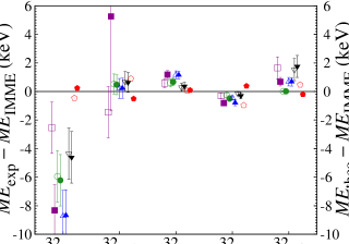
Figure 14: (Color online) Deviations of experimental or theoretical masses of the $A=32$ quintet from the corresponding quadratic IMME fit. (Purple) squares are quoted from Ref. Triambak et al. (2006). (Purple) filled squares are quoted from Ref. Kwiatkowski et al. (2009). (Green) circles are quoted from Ref. Kankainen et al. (2010), Table 8, set A; (green) filled circles are from set B; up (blue) triangles are from set C; up (blue) filled triangles are from set D; down (black) triangles are from set E; down (black) filled triangles are from set F. The recent theoretical work of Signoracci and Brown  Signoracci and Brown (2011) is presented as (red) pentagons; whereas (red) filled pentagons are present calculation.

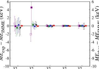
Figure 15: (Color online) Deviations of experimental or theoretical masses of the $A=32$ quintet from the corresponding cubic IMME fit. Refer to Fig. 14 for description.

Before we discuss any evidence for non-zero $d$ or $e$ coefficients, let us compare the values of the corresponding $b$ and $c$ coefficients. As seen from Table 7, $b$ coefficients obtained in the present work reproduce much better the experimental values compared to the results of Ref. Signoracci and Brown (2011). In particular, we get all deviations smaller than 10 keV, while the calculations of Ref. Signoracci and Brown (2011) result in much larger deviations of $\scriptstyle\mathtt{\sim}$50 keV. This is due to the fact that the corresponding mass differences $(M_{-2}-M_{2})$ deviate from the experimental value by about 207 keV, while the mass differences $(M_{1}-M_{-1})$ are different from the experimental value by about 107 keV (see Table 6). The present INC Hamiltonian produces mass differences which deviate at most by 20 keV from the experimental values and thus results in very close $b$ values. This discrepancy should be kept in mind when comparing the values of the predicted $d$ coefficient with the experimental value.

Let us remark that the theoretical $b$ coefficients calculated via an exact diagonalization almost coincide with the $b$ coefficients listed in Table 15, which were obtained in a fit (within perturbation theory). That means, the perturbation theory used in section  II provides a very good approximation to the $b$ coefficients.

Overall the $c$ coefficients predicted by both models are close to experimental values, with a maximum $\scriptstyle\mathtt{\sim}$2 keV for the present results and $\scriptstyle\mathtt{\sim}$4 keV for the values of Ref. Signoracci and Brown (2011).

Each set of IMME coefficients in Table 7 is ended by the $\chi^{2}/n$ value characterizing the quality of the fit. It is seen that all calculations agree well with the experimental conclusion that the cubic form of the IMME describes best the nuclear mass trend of the lowest $0^{+}$ quintet in $A=32$, since it produces the lowest $\chi^{2}/n$ value (with the exception of the USDA interaction, see explanation below). The quartic IMME with $d=0$ is worse than the cubic one (again, except for the prediction of the USDA interaction).

To illustrate this effect, we plot in Fig. 14 and Fig. 15 deviations of nuclear mass excesses from the best IMME fit values, assuming a quadratic and a cubic form of the IMME, respectively. These figures include different experimental data sets and two different theoretical calculations of mass excesses (Ref. Signoracci and Brown (2011) and present work). It is obvious that the best fit is produced by a cubic form of the IMME (Fig. 15).

The values of the corresponding $d$ coefficient are, however, different in experimental and theoretical analysis. The experimental value ranges from 0.51 keV to 1.00 keV for various sets of experimental data (see Table 8). Taken the adopted values of experimental mass excesses, we get $d_{exp}=0.89(11)$ keV (from our recent compilation  Lam et al. (bles)). At the same time, theoretical values obtained from the USD interaction are $d_{th}=0.39$ keV Signoracci and Brown (2011) and $d_{th}=-0.19$ keV (present result). The USDB interaction results in much smaller $\chi^{2}/n$ values for all fits, with the minimum again for a cubic form of the IMME. The corresponding $d$ coefficients are $d_{th}=0.28$ keV Signoracci and Brown (2011) and $d_{th}=-0.07$ keV (present result).

Let us remark that although the $d$-values of Ref. Signoracci and Brown (2011) are closer to the experimental one, there is an essential discrepancy in their theoretical $b$ coefficients, especially for the USDB interaction. At the same time, although being in better agreement for $b$ coefficients, our calculations point towards a negative value of the $d$ coefficient. We think that this is due to a peculiarity of the fit, since the sign of the $d$ coefficient is determined by a ratio of mass differences $(M_{-2}-M_{2})/(M_{1}-M_{-1})$ (see Eq. (45d)). To get a zero value for the $d$ coefficient, this ratio should be equal to 2. The ratio we get with the USD interaction is $~{}2.00019$, resulting in a negative $d$ value, while the USD calculation of Ref. Signoracci and Brown (2011) produces a ratio of $~{}1.99957$, which is closer to the experimental ratio of $~{}1.99902$ and both producing a positive $d$ value.

As was shown by Signoracci and Brown Signoracci and Brown (2011), the shell-model value of the $d$ coefficient relates to the degree of the isospin-mixing in the initial and final nuclear states. For this reason, the calculation with the USDA interaction should be taken with caution, since accidentally there is a very closely lying state $0^{+}$, $T=0$ in the vicinity of the IAS $0^{+}$, T=2 state in ³²S Signoracci and Brown (2011) and thus an unrealistic value for the $e$ coefficient. We arrive at a similar conclusion while adding our parametrization of the INC Hamiltonian to the USDA interaction.

Apparently, the effects discussed in this section require a very high precision of relevant experimental data and theoretical accuracy. In particular, the experimental determination of the position of $0^{+}$ states in the vicinity of the IAS in ³²Cl and ³²P could certainly help to refine the prediction of the $d$ coefficient. Furthermore, the essential uncertainty of ³²Ar mass may affect both experimental conclusions and theoretical description. Hence, a direct re-measurement of the ³²Ar mass would shed light on this issue.

Table 8: Comparison of theoretical $d$ coefficients with experimental values for the $A=32$ quintet.

Experimental and Theoretical Works	$d$ (keV)	${\chi^{2}}/{n_{\textnormal{quadr.}}}$	${\chi^{2}}/{n_{\textnormal{cubic}}}$
Triambak S. et. al.  Triambak et al. (2006)	0.54 (16)	6.5	0.77
Kwiatkowski S. et. al.  Kwiatkowski et al. (2009)	1.00 (9)	30.6	0.48
Set A from Kankainen A. et. al.  Kankainen et al. (2010)	0.52 (12)	9.9	0.86
Set B Ibid.	0.60 (13)	12.3	0.31
Set C Ibid.	0.90 (12)	28.3	0.002
Set D Ibid.	1.00 (13)	30.8	0.09
Set E Ibid.	0.51 (15)	6.5	0.74
Set F Ibid.	0.62 (16)	8.3	0.28
Signoracci A. & Brown B. A.  Signoracci and Brown (2011) (USD)	0.39	1.09	0.005
Present work	$-0.19$	0.26	0.02

Table 9: Comparison of $\delta_{\textnormal{IM}}$ values.

Nuclear	Parent	Present Work					Previous Work
Hamiltonian	Nucleus			Jastrow-type SRC function			Ormand &	Towner &
		w/o SRC	UCOM	Argonne V18	CD-Bonn	Miller	Brown	Hardy
						Spencer
USD
	22Mg	0.021	0.022	0.021	0.021	0.023	0.017	0.010 (10)
	26Alm	0.011	0.012	0.012	0.011	0.013	0.01	0.025 (10)
	26Si	0.046	0.046	0.046	0.046	0.046	0.028	0.022 (10)
	30S	0.026	0.028	0.027	0.025	0.030	0.056	0.137 (20)
	34Cl	0.037	0.037	0.036	0.036	0.036	0.06	0.091 (10)
	34Ar	0.005	0.006	0.006	0.006	0.007	0.008	0.023 (10)
USDA
	22Mg	0.021	0.022	0.021	0.020	0.024
	26Alm	0.012	0.013	0.013	0.012	0.015
	26Si	0.041	0.042	0.042	0.041	0.043
	30S	0.020	0.022	0.021	0.020	0.024
	34Cl	0.031	0.032	0.031	0.031	0.032
	34Ar	0.006	0.007	0.007	0.006	0.008
USDB
	22Mg	0.021	0.022	0.021	0.021	0.023
	26Alm	0.012	0.013	0.013	0.013	0.015
	26Si	0.044	0.045	0.044	0.044	0.046
	30S	0.025	0.026	0.025	0.024	0.028
	34Cl	0.036	0.036	0.035	0.035	0.035
	34Ar	0.005	0.005	0.005	0.005	0.006

Table 10: Comparison of $\mathscr{F}t$ values.

						$\mathscr{F}t$ (s)
Parent	Exp. $ft$ (s)	Corrections (%)				Present	Towner &
Nucleus		$\delta_{\textnormal{IM}}$	$\delta_{\textnormal{RO}}$	$\delta^{\prime}_{\textnormal{R}}$	$\delta_{\textnormal{NS}}$	work	Hardy
22Mg	3052    (7)	0.0216 (9)	0.370 (20)	1.466 (17)	$-0.225$ (20)	3077.6 (72)	3077.6 (74)
26Alm	3036.9 (9)	0.0120 (8)	0.280 (15)	1.478 (20)	0.005 (20)	3072.9 (13)	3072.4 (14)
34Cl	3049.4 (12)	0.0363 (5)	0.550 (45)	1.443 (32)	$-0.085$ (15)	3072.6 (21)	3070.6 (21)
34Ar	3053    (8)	0.0060 (4)	0.635 (55)	1.412 (35)	$-0.180$ (15)	3070.7 (84)	3069.6 (85)

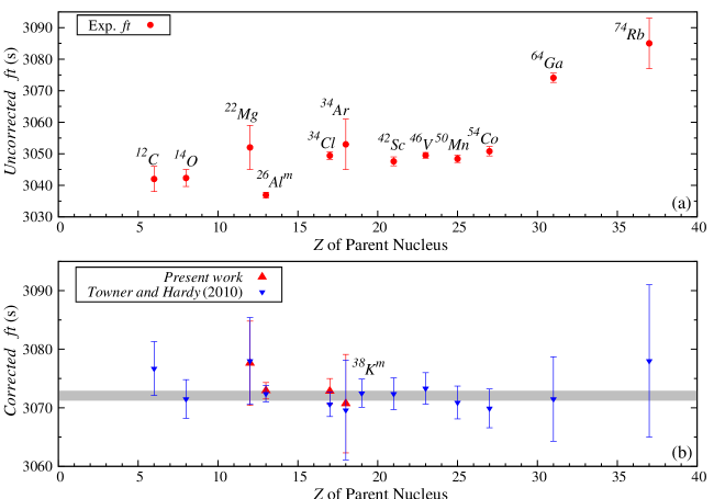
Figure 16: (Color online) Comparison of $\mathscr{F}t$ values in $sd$-shell space. Plot (a) depicts experimental $ft$ values. The $ft$ value of ${}^{38}K^{m}$ is not shown, it is 3051.9 (10) s. Plot (b) shows $\mathscr{F}t$ values. Horizontal (grey) strip is 1 standard deviation according to Ref.Towner and Hardy (2010).

Table 11: Values of $\delta_{\textnormal{IM}}$ for Fermi $\beta$ transitions between non-analog states (from the lowest $0^{+},T=1$ state of ³⁴Ar or ³⁴Cl to the first excited $0^{+},T=1$ state of the corresponding daughter nuclei).

	Nuclear	Present Work						Previous Work
	Hamiltonian
		w/o SRC	UCOM	Jastrow type SRC function
				Argonne V18	CD-Bonn	Miller	Strengths from	Ormand &
						Spencer	Ref. Ormand and Brown (1989a)	Brown  Ormand and Brown (1985)
$\delta_{\textnormal{IM}}\times 10^{5}$ :
34Ar
	USD	$-37.97$	$-8.843$	$-29.69$	$-48.19$	$-27.44$	$-361.2$	$-3.5$
	USDA	$-127.8$	$-101.2$	$-118.9$	$-140.2$	$-71.25$	—	—
	USDB	$-134.1$	$-120.8$	$-134.5$	$-142.9$	$-106.1$	—	—
$\delta_{\textnormal{IM}}\times 10^{2}$ :
34Cl
	USD	$-3.103$	$-3.098$	$-3.061$	$-3.071$	$-3.061$	$-3.960$	$-2.7$
	USDA	$-2.734$	$-2.730$	$-2.697$	$-2.712$	$-2.695$	—	—
	USDB	$-3.120$	$-3.115$	$-3.076$	$-3.088$	$-3.071$	—	—

VI Isospin-Symmetry Breaking and Fermi Beta Decay

VI.1 Superallowed Fermi beta decay

The absolute $\mathscr{F}t$ value of a superallowed $0^{+}\to 0^{+}$ $\beta$-decay can be deduced from the experimental $ft$ value applying various corrections (see Ref. Towner and Hardy (2010) and references therein), i.e.

$$\mathscr{F}t =ft(1+\delta^{\prime}_{\textnormal{R}})(1+\delta_{\textnormal{NS}}-\delta_{C})$$ (46)

$$=\frac{K}{G_{V}^{2}|M_{F0}|^{2}(1+\Delta_{R}^{V})}\,,$$

where $\Delta_{R}^{V}$, $\delta^{\prime}_{\textnormal{R}}$, and $\delta_{\textnormal{NS}}$ are transition-independent, transition-dependent and structure-dependent parts of the radiative correction, respectively, while $\delta_{C}$ is the nuclear structure correction due to the isospin-symmetry breaking in the parent and daughter nuclear states. Other constants in this expression are

$$K =2\pi^{3}\hbar\,ln2/(m_{e}c^{2})^{5}$$

$$=(8120.278\pm 0.0004)\times 10^{-10}\textnormal{GeV}^{-4}\textnormal{s}\,,$$

$G_{V}$ is the vector coupling constant for a semileptonic weak process, while

$$|M_{F0}|^{2}=|\langle\psi_{f}|T_{+}|\psi_{i}\rangle|^{2}=T(T+1)-T_{zi}T_{zf}$$

is the value of the Fermi matrix element squared in the isospin-symmetry limit, which in the case of $T=1$ emitters is $|M_{F0}|^{2}=2$.

Provided the absolute $\mathscr{F}t$ value of superallowed $0^{+}\to 0^{+}$ $\beta$ transitions is constant as stated by the CVC hypothesis, the $G_{V}$ value can be deduced from Eq. (46) and then the $V_{ud}$ CKM matrix element can be obtained from comparison of $G_{V}$ with the vector coupling constant extracted from the muon decay.

The isospin-symmetry breaking correction is defined as a deviation of the realistic Fermi matrix element from its model-independent value:

$$|M_{F}|^{2}=|M_{F0}|^{2}(1-\delta_{C})\,.$$ (47)

Within the shell model, the initial and final nuclear states represent a mixing of many-body spherical harmonic-oscillator configurations. In practice, the isospin-symmetry breaking correction to $|M_{F0}|^{2}$ is usually separated in two terms: $\delta_{C}=\delta_{\textnormal{IM}}+\delta_{\textnormal{RO}}$ (we adopt here the notations of Ormand and Brown Ormand and Brown (1985, 1989b); in the work of Towner and Hardy Towner and Hardy (2002); Hardy and Towner (2005); Towner and Hardy (2008, 2010), these terms are referred to as $\delta_{C1}$ and $\delta_{C2}$, respectively). The first term, $\delta_{\textnormal{IM}}$, is a correction to the Fermi matrix element $M_{F0}$ from the isospin-symmetry breaking in the configuration mixing of the spherical harmonic-oscillator basis functions (isospin-mixing correction). This is obtained via the diagonalization of an effective INC Hamiltonian within the valence space. The second term, $\delta_{\textnormal{RO}}$, arises in the calculation of transition matrix elements due to the non-unity of the radial overlap of proton and neutron wave functions (radial-overlap correction). To get it, one has to replace the harmonic-oscillator single-particle wave functions by more realistic spherically-symmetric wave functions obtained from a better suited finite-well plus Coulomb potential (to account for the isospin non-conservation outside the model space).

In the present paper, we present calculations of the isospin-mixing corrections $\delta_{\textnormal{IM}}$ to the experimental $ft$ values for $0^{+}\to 0^{+}$ $\beta$ transitions in $sd$-shell nuclei. Although this correction is known to be quite small (from $\scriptstyle\mathtt{\sim}$0.01% to $\scriptstyle\mathtt{\sim}$0.1%), we can still see noticeable changes to the absolute $\mathscr{F}t$ values compared to the existing evaluation, based on the calculations of Towner and Hardy Towner and Hardy (2010).

The values of $\delta_{\textnormal{IM}}$ obtained from the USD, USDA and USDB interactions with $V_{coul}+V_{0}$ INC Hamiltonian with all possible approaches to the SRC in Coulomb TBME’s are summarized in Table 9. In the last two columns, we give for comparison the values from the previous work by Ormand and Brown Ormand and Brown (1989b) and the most recent results of Towner and Hardy Towner and Hardy (2008).

As seen from the table, in spite of different interactions used, our calculations lead to very consistent values for various isotopes. Only for ²⁶Si and ³⁰S, the USDA interaction results in somewhat smaller values of corrections than those predicted by the USD or USDB. The dependence on one or another approach to the SRC is also marginal. For most isotopes, the Miller and Spencer parametrization produces slightly larger values of corrections.

If we compare our results with those obtained by Ormand and Brown, we see that for ²²Mg, ²⁶Al^m and ³⁴Ar there is a good agreement. However, clear differences can be noticed for ²⁶Si, ³⁰S and ³⁴Cl. We get a larger value for the former and almost twice smaller values for the two latter cases. Regarding the calculation of Towner and Hardy (last column), only for the two lightest emitters (²²Mg and ²⁶Al^m) our values are close to their range (uncertainties included). For the rest of the nuclei, there is an essential discrepancy — we get a larger value for ²⁶Si and much smaller values for the heavier emitters. The main difference in the approaches is that the authors of Ref. Towner and Hardy (2008) adjusted INC Hamiltonian strength parameters separately for each considered multiplet (case by case) to reproduce the isobaric mass splitting, while in our work and that of Ref. Ormand and Brown (1989b) a global parametrization for $sd$-shell nuclei has been exploited.

In Table 10 we apply the calculated values of $\delta_{\textnormal{IM}}$ to deduce a new set of $\mathscr{F}t$ values for four best known $sd$-shell emitters. The present estimation is based on the USD calculation with $V_{coul}$ plus $V_{0}$ INC Hamiltonian, taken the average of the results obtained for various approaches to SRCs. The experimental $ft$ values and the other corrections ($\delta_{\textnormal{RO}}$, $\delta^{\prime}_{\textnormal{R}}$ and $\delta_{\textnormal{NS}}$) are taken from Ref. Towner and Hardy (2010).

It is seen that for ³⁴Cl and ³⁴Ar, the deduced values are somewhat different from those adopted currently by Towner and Hardy. The implementation of our $sd$-shell results on $\delta_{IM}$ is illustrated in Fig. 16, where corrected values of the 13 best known emitters from Ref. Towner and Hardy (2010) are shown. Further analysis and calculation of the radial-overlap corrections is under way.

VI.2 Fermi Beta Decay to Non-Analogue States

If the isospin-symmetry is broken, the Fermi beta decay between non-analogue $0^{+}$ states may take place. These transitions are of great interest since their rate is directly related to the degree of the isospin-mixing and it can help to test the model predictions Hagberg et al. (1994). Unfortunately, no experimental data are known for the $sd$-shell nuclei. However, we can explore the sensitivity of the matrix element of the non-analogue transitions (its isospin-mixing part) to the details of the shell-model Hamiltonian. In this context, we have performed calculations for two cases of ³⁴Cl and ³⁴Ar, considered before by Ormand and Brown in Ref. Ormand and Brown (1985). The results are shown in Table 11, where we present calculations of $\delta_{IM}$ for Fermi $\beta$-transitions from the lowest $0^{+}$ state in ³⁴Cl or in ³⁴Ar to the first excited $0^{+}$ state in the respective daughter nuclei. Present calculations are based on the $V_{coul}$ plus $V_{0}$ INC Hamiltonian with strength parameters from Table 5 (Range I).

It is interesting to see that the values predicted for ³⁴Cl by various interactions, including the early work of Ormand and Brown, are quite consistent, being roughly $-2.7$ — $-3.1$ $\times 10^{-2}$. However, the magnitudes of corrections predicted for a decay of ³⁴Ar are much smaller and probably because of the sensitivity to the details of the calculations. Our result spread in a wide range between $-8.8\times 10^{-5}$ and $-48.2\times 10^{-5}$ for USD interaction and between $-0.7\times 10^{-3}$ and $-1.4\times 10^{-3}$ for USDA/USDB interactions. The value given in Ref. Ormand and Brown (1985) is the smallest among the values, $-3.5\times 10^{-5}$, while the parameters from Ref. Ormand and Brown (1989a) result contrary in the largest number, $-3.6\times 10^{-3}$. It would be very interesting and useful to have experimental data to make a critical selection between different predictions.

VII Summary and Conclusions

In conclusion, we have presented a set of new empirical INC Hamiltonians in the $sd$ shell-model space which accurately reproduces the isobaric mass splittings. The fitting procedure used in our work is close to that used earlier by Ormand and Brown, however, an advanced study of the harmonic oscillator parameters, modern approaches to SRCs, as well as, an updated and largely extended experimental database and full $sd$-shell space calculations have been performed. In our model, besides a one-body term, an effective $T=1$ component of the isospin-conserving interaction or the Wigner term of the pion and $\rho$-meson exchange potentials have been exploited to model effective charge-dependent forces of nuclear origin. More sophisticated forms of those forces could be explored as well. The parameters of the INC part of the Hamiltonian were adjusted in a fit, designed to reproduce the known $b$ and $c$ coefficients of the IMME. Different types of the isospin-conserving interaction and various procedures to account for the SRC’s lead to rather similar magnitudes of the rms deviations, with the best values around ${\raise 0.73193pt\hbox{$\scriptstyle\mathtt{\sim}$}}32$ keV for rms of $b$ coefficients and ${\raise 0.73193pt\hbox{$\scriptstyle\mathtt{\sim}$}}9$ keV for rms of $c$ coefficients. The quality of the fit and the Coulomb strength parameters unambiguously suggest that in order to reproduce the experimental IMME coefficients, the electromagnetic interaction should be supplemented by nuclear charge-dependent forces.

We believe that the constructed INC Hamiltonians can provide a high accuracy in the description of the isospin-symmetry forbidden processes. A few applications have been considered here with the purpose to demonstrate new features. First, we have been able to propose a quantitative description of a staggering effect of the IMME $b$ and $c$ coefficients as a function of the mass number. This allowed us to conclude on the contribution of the Coulomb and nuclear charge-dependent forces to pairing.

Second, we studied the validity of the IMME equation beyond the quadratic form in the lowest $A=32$ quintet. Our calculations point towards the existence of a non-zero $d$ coefficient in agreement with experimental data. The predicted values turn out to be very sensitive to the shell-model Hamiltonian used and thus more precise and more extensive data which may help to constrain theoretical parameters will be of great importance.

Third, we present a new set of isospin-mixing corrections to $sd$-shell $0^{+}\to 0^{+}$ beta decay rates. All Hamiltonians provide surprisingly similar results, however, different from the values of Towner and Hardy. A more advanced study of these corrections should be performed.

Finally, preliminary calculations of the isospin-mixing corrections to the Fermi beta decay between non-analogue states suggest that these rates might be sensitive to the details of an INC Hamiltonian and thus could serve as a perfect test to a theoretical description.

As a general conclusion, we hope that the Hamiltonian will be of large use and we intend to perform numerous applications to understand better predictions and differences between various INC parametrizations. Similar study has been performed for $psd$, $sdpf$, and $pf$ model spaces, the results and various applications will be published elsewhere  Lam et al. (tion). More extended and more precise experimental data on isobaric masses, as well as measurements of the isospin-forbidden decay rates would be very helpful to test further and to refine our model.

Appendix A Fitted $b$ and $c$ Coefficients

Table 12: Comparison between fitted $b$ coefficients with experimental values of $T=1/2$ doublets in $sd$-shell nuclei.

mass, $A$	$J^{\pi}$	$b$ (exp)	$b$ (fit)	References
		(keV)	(keV)
19	$\frac{1}{2}^{+}$	4021.85 (16)	4032.88	Audi and Wang (2012); Tilley et al. (1995)
	$\frac{5}{2}^{+}$	4062.97 (19)	4024.27
	$\frac{3}{2}^{+}$	4003.8   (4)	3978.8
21	$\frac{3}{2}^{+}$	4329.49 (28)	4311.36	Audi and Wang (2012); Firestone (2004)
	$\frac{5}{2}^{+}$	4310.66 (30)	4303.46
	$\frac{7}{2}^{+}$	4299.7   (4)	4310.7
23	$\frac{3}{2}^{+}$	4838.94 (69)	4850.43	Audi and Wang (2012); Firestone (2007)
	$\frac{5}{2}^{+}$	4849.66 (70)	4855.31
	$\frac{7}{2}^{+}$	4815.1   (11)	4829.6
25	$\frac{5}{2}^{+}$	5058.94 (48)	5067.73	Audi and Wang (2012); Firestone (2009)
27	$\frac{5}{2}^{+}$	5594.71 (18)	5563.80	Audi and Wang (2012); Endt (1998)
	$\frac{1}{2}^{+}$	5531.8   (3)	5551.4
	$\frac{3}{2}^{+}$	5537.5   (3)	5570.8
29	$\frac{1}{2}^{+}$	5724.8   (6)	5752.7	Audi and Wang (2012); Endt (1998)
	$\frac{3}{2}^{+}$	5835.0   (6)	5760.3
31	$\frac{1}{2}^{+}$	6179.87 (98)	6118.13	Audi and Wang (2012); Endt (1998)
	$\frac{3}{2}^{+}$	6162.6   (10)	6103.9
33	$\frac{3}{2}^{+}$	6364.93 (44)	6324.10	Audi and Wang (2012); Endt (1998)
	$\frac{1}{2}^{+}$	6334.50 (47)	6340.58
35	$\frac{3}{2}^{+}$	6748.48 (75)	6723.59	Audi and Wang (2012); Endt (1998)
	$\frac{1}{2}^{+}$	6713.22 (80)	6709.4
	$\frac{5}{2}^{+}$	6736.1   (8)	6710.3
	$\frac{3}{2}^{+}$	6692.7   (8)	6705.4
	$\frac{5}{2}^{+}$	6728.97 (77)	6656.38
	$\frac{1}{2}^{+}$	6665      (10)	6648
37	$\frac{3}{2}^{+}$	6929.82 (23)	6897.54	Audi and Wang (2012); Endt (1998)
	$\frac{1}{2}^{+}$	6890.85 (25)	6899.81
	$\frac{5}{2}^{+}$	6884.0   (4)	6947.5
39	$\frac{3}{2}^{+}$	7306.84 (60)	7321.70	Audi and Wang (2012); Singh and Cameron (2006)
	$\frac{1}{2}^{+}$	7252.8   (11)	7360.4

Table 13: Comparison between fitted $b$- and $c$ coefficients with experimental values of $T=1$ triplets in $sd$-shell nuclei.

mass, $A$	$J^{\pi}$	$b$ (exp)	$b$ (fit)	$c$ (exp)	$c$ (fit)	References
		(keV)	(keV)	(keV)	(keV)
18	$0^{+}$	3832.57 (18)	3842.20	352.74 (50)	339.31	Audi and Wang (2012); Tilley et al. (1995)
	$2^{+}$	3785.2   (2)	3795.9	267.1   (5)	268.4
20	$2^{+}$	4216.2   (5)	4184.2	185.1   (20)	193.7	Audi and Wang (2012); Tilley et al. (1998)
	$3^{+}$	4186      (4)	4184	200      (5)	212
	$4^{+}$	4206      (4)	4169	181      (5)	186
22	$0^{+}$	4594.74 (16)	4583.96	312.03 (26)	297.64	Audi and Wang (2012); Firestone (2005)
	$2^{+}$	4580.96 (16)	4577.16	277.86 (28)	266.02
	$4^{+}$	4570.0   (2)	4579.4	230.6   (4)	230.0
	$2^{+}$	4567.8   (3)	4581.0	224.1   (20)	235.8
24	$4^{+}$	4966.88 (50)	4956.56	183.86 (50)	196.91	Audi and Wang (2012); Firestone (2007)
	$1^{+}$	4943.7   (5)	4960.9	182.0   (5)	191.6
	$2^{+}$	4941      (2)	4969	179      (2)	164
26	$0^{+}$	5319.13 (6)	5315.50	304.05 (9)	308.03	Audi and Wang (2012); Endt (1998)
	$2^{+}$	5312.7   (12)	5337.5	265.2   (1)	273.7
28	$3^{+}$	5633.06 (55)	5654.87	177.11 (56)	192.05	Audi and Wang (2012); Endt (1998)
	$2^{+}$	5670.57 (55)	5655.02	179.61 (56)	186.36
30	$0^{+}$	5967.64 (150)	5961.08	275.93 (153)	272.91	Audi and Wang (2012); Basunia (2010)
	$2^{+}$	5955.3   (15)	5944.0	238.4   (16)	239.9
	$2^{+}$	5919.7   (15)	5941.3	220.7   (16)	229.8
32	$1^{+}$	6267.2   (5)	6235.6	194.1   (6)	199.8	Audi and Wang (2012); Endt (1998)
	$2^{+}$	6273.1   (5)	6232.9	164.2   (11)	169.7
	$0^{+}$	6243.9   (5)	6233.9	149.2   (11)	153.2
34	$0^{+}$	6559.48 (17)	6559.55	285.50 (18)	271.69	Audi and Wang (2012); Endt (1998)
	$2^{+}$	6541.2   (2)	6542.3	236.8   (3)	234.8
	$2^{+}$	6551.1   (3)	6565.3	198.1   (4)	204.3
	$0^{+}$	6537      (1)	6574	239      (1)	230
36	$2^{+}$	6834.7   (2)	6859.3	150.9   (3)	148.0	Audi and Wang (2012); Endt (1998)
	$3^{+}$	6845      (1)	6861	224      (1)	220
	$1^{+}$	6808.4   (3)	6854.1	190.2   (6)	196.0
	$1^{+}$	6843.5   (3)	6845.1	239.9   (7)	235.8
38	$0^{+}$	7110.5   (2)	7153.9	283.7   (4)	268.6	Audi and Wang (2012); Cameron and Singh (2008)
	$2^{+}$	7133.22 (18)	7102.99	203.39 (35)	195.29

Table 14: Comparison between fitted $b$ and $c$ coefficients with experimental values of $T=3/2$ quartets in $sd$-shell nuclei.

mass, $A$	$J^{\pi}$	$b$ (exp)	$b$ (fit)	$c$ (exp)	$c$ (fit)	References
		(keV)	(keV)	(keV)	(keV)
19	$\frac{5}{2}^{+}$	3982.7   (40)	3930.6	240.7   (22)	233.6	Audi and Wang (2012); Tilley et al. (1995)
	$\frac{3}{2}^{+}$	3987.3   (50)	3930.4	230.8   (27)	231.4
21	$\frac{5}{2}^{+}$	4444.5   (22)	4384.5	243.1   (18)	230.6	Audi and Wang (2012); Firestone (2004)
	$\frac{1}{2}^{+}$	4399.6   (23)	4380.5	216.8   (19)	225.9
23	$\frac{5}{2}^{+}$	4749.72 (12)	4757.64	225.99 (10)	223.86	Audi and Wang (2012); Firestone (2007)
25	$\frac{5}{2}^{+}$	5174.1   (18)	5171.6	219.9   (11)	225.0	Audi and Wang (2012); Firestone (2009)
27	$\frac{1}{2}^{+}$	5406.8   (29)	5477.2	210.4   (16)	226.7	Audi and Wang (2012); Endt (1998)
29	$\frac{5}{2}^{+}$	5812.5   (55)	5820.8	209.4   (50)	214.1	Audi and Wang (2012); Endt (1998)
31	$\frac{3}{2}^{+}$	6069.7   (87)	6042.6	199.1   (45)	207.1	Audi and Wang (2012); Endt (1998)
	$\frac{1}{2}^{+}$	6046.8   (127)	6049.1	183.9   (65)	210.6
33	$\frac{1}{2}^{+}$	6433.41 (33)	6397.39	209.82 (33)	209.98	Audi and Wang (2012); Endt (1998)
35	$\frac{3}{2}^{+}$	6673.14 (17)	6652.29	202.08 (14)	199.06	Audi and Wang (2012); Endt (1998)
37	$\frac{3}{2}^{+}$	6990.94 (26)	6981.57	203.03 (48)	198.41	Audi and Wang (2012); Endt (1998)
	$\frac{1}{2}^{+}$	6953.6   (55)	6971.9	214.2   (56)	212.0

Table 15: Comparison between fitted $b$ and $c$ coefficients with experimental values of $T=2$ quintets in $sd$-shell nuclei.

mass, $A$	$J^{\pi}$	$b$ (exp)	$b$ (fit)	$c$ (exp)	$c$ (fit)	References
		(keV)	(keV)	(keV)	(keV)
20	$0^{+}$	4220.5   (37)	4180.1	245.0   (18)	234.0	Audi and Wang (2012); Tilley et al. (1998)
24	$0^{+}$	4961.2   (9)	4963.4	225.9   (4)	225.3	Audi and Wang (2012); Firestone (2007); Wrede et al. (2010)
28	$0^{+}$	5589.8   (19)	5646.7	215.5   (12)	219.1	Audi and Wang (2012); Endt (1998); Wrede et al. (2010)
32	$0^{+}$	6254.19 (27)	6235.70	208.55 (14)	208.27	Audi and Wang (2012); Endt (1998)
36	$0^{+}$	6828.0   (19)	6864.9	201.3   (6)	199.4	Audi and Wang (2012); Endt (1998)

References

- Machleidt and Entem (2011) R. Machleidt and D. R. Entem, Phys. Rep. 503, 1 (2011).
- Miller et al. (1990) G. A. Miller, B. M. K. Nefkens, and I. Slaus, Phys. Rep. 194, 1 (1990).
- Machleidt (2001) R. Machleidt, Phys. Rev. C 63, 024001 (2001).
- Epelbaum et al. (2009) E. Epelbaum, H.-W. Hammer, and Ulf.-G. Meißner, Rev. Mod. Phys. 81, 1773 (2009).
- Towner and Hardy (2010) I. S. Towner and J. C. Hardy, Rep. Prog. Phys. 73, 046301 (2010).
- Hardy and Towner (2009) J. C. Hardy and I. S. Towner, Phys. Rev. C 79, 055502 (2009).
- Naviliat-Cuncic and Severijns (2009) O. Naviliat-Cuncic and N. Severijns, Phys. Rev. Lett. 102, 142302 (2009).
- Towner (1973) I. S. Towner, Nucl. Phys. A 216, 589 (1973).
- Smirnova and Volpe (2003) N. A. Smirnova and C. Volpe, Nucl. Phys. A 714, 441 (2003).
- Bentley and Lenzi (2007) M. A. Bentley and S. Lenzi, Prog. Part. Nucl. Phys. 59, 497 (2007).
- Blank and Borge (2008) B. Blank and M. J. G. Borge, Prog. Part. Nucl. Phys. 60, 403 (2008).
- Hagberg et al. (1994) E. Hagberg, V. T. Koslowsky, J. C. Hardy, I. S. Towner, J. G. Hykawy, G. Savard, and T. Shinozuka, Phys. Rev. Lett. 73, 396 (1994).
- Farnea et al. (2004) E. Farnea et al., Phys. Lett. B 551, 56 (2004).
- Orlandi et al. (2009) R. Orlandi et al., Phys. Rev. Lett. 103, 052501 (2009).
- Blin-Stoyle and Rosina (1965) R. J. Blin-Stoyle and M. Rosina, Nucl. Phys. 70, 321 (1965).
- Jänecke (1969) J. Jänecke, Systematics of Coulomb Energies and Excitation Energies of Isobaric Analogue States, Isospin in Nuclear Physics, edited by D. H. Wilkinson (North-Holland, Amsterdam, 1969) p. 297.
- Bertsch and Wildenthal (1973) G. F. Bertsch and B. H. Wildenthal, Phys. Rev. C 8, 1023 (1973).
- Blin-Stoyle (1969) R. J. Blin-Stoyle, Isospin in Nuclear -Decay, Isospin in Nuclear Physics, edited by D. H. Wilkinson (North-Holland, Amsterdam, 1969) p. 115.
- Towner and Hardy (1973) I. S. Towner and J. C. Hardy, Nucl. Phys. A 205, 33 (1973).
- Ormand and Brown (1985) W. E. Ormand and B. A. Brown, Nucl. Phys. A 440, 274 (1985).
- Ormand and Brown (1989a) W. E. Ormand and B. A. Brown, Nucl. Phys. A 491, 1 (1989a).
- Zuker et al. (2002) A. P. Zuker, S. M. Lenzi, G. Martínez-Pinedo, and A. Poves, Phys. Rev. Lett. 89, 142502 (2002).
- Ormand and Brown (1989b) W. E. Ormand and B. A. Brown, Phys. Rev. Lett. 62, 866 (1989b).
- Towner and Hardy (2008) I. S. Towner and J. C. Hardy, Phys. Rev. C 77, 025501 (2008).
- Ormand and Brown (1986) W. E. Ormand and B. A. Brown, Phys. Lett. B 174, 128 (1986).
- Brown (1990) B. A. Brown, Phys. Rev. Lett. 65, 2753 (1990).
- Brown (1991) B. A. Brown, Phys. Rev. C 43, R1513 (1991).
- Ormand (1996) W. E. Ormand, Phys. Rev. C 53, 214 (1996).
- Ormand (1997) W. E. Ormand, Phys. Rev. C 55, 2407 (1997).
- Cole (1996) B. J. Cole, Phys. Rev. C 54, 1240 (1996).
- Hamamoto and Sagawa (1993) I. Hamamoto and H. Sagawa, Phys. Rev. C 48, R960 (1993).
- Dobaczewski and Hamamoto (1995) J. Dobaczewski and I. Hamamoto, Phys. Lett. B 345, 181 (1995).
- Colo et al. (1995) G. Colo, M. A. Nagarajan, P. Van Isacker, and A. Vitturi, Phys. Rev. C 52, R1175 (1995).
- Sagawa et al. (1996) H. Sagawa, N. Van Giai, and T. Suzuki, Phys. Rev. C 53, 2163 (1996).
- Liang et al. (2009) H. Liang, N. V. Giai, and J. Meng, Phys. Rev. C 79, 064316 (2009).
- Satula et al. (2009) W. Satula, J. Dobaczewski, W. Nazarewicz, and M. Rafalski, Phys. Rev. Lett. 103, 012502 (2009).
- Satula et al. (2011) W. Satula, J. Dobaczewski, W. Nazarewicz, and M. Rafalski, Phys. Rev. Lett. 106, 132502 (2011).
- Petrovici et al. (2008) A. Petrovici, K. W. Schmid, O. Radu, and A. Faessler, Phys. Rev. C 78, 064311 (2008).
- Caurier et al. (2002) E. Caurier, P. Navratil, W. E. Ormand, and J. P. Vary, Phys. Rev. C 66, 024314 (2002).
- Michel et al. (2010) N. Michel, W. Nazarewicz, and M. Ploszajczak, Phys. Rev. C 82, 044315 (2010).
- Auerbach (2009) N. Auerbach, Phys. Rev. C 79, 035502 (2009).
- Auerbach (2010) N. Auerbach, Phys. Rev. C 81, 067305 (2010).
- Caurier et al. (2005) E. Caurier, G. Martínez-Pinedo, F. Nowacki, A. Poves, and A. P. Zuker, Rev. Mod. Phys. 77, 427 (2005).
- Brown and Richter (2006) B. A. Brown and W. A. Richter, Phys. Rev. C 74, 034315 (2006).
- Honma et al. (2004) M. Honma, T. Otsuka, B. A. Brown, and T. Mizusaki, Phys. Rev. C 69, 034335 (2004).
- Nowacki and Poves (2009) F. Nowacki and A. Poves, Phys. Rev. C 79, 014310 (2009).
- Roth et al. (2010) R. Roth, T. Neff, and H. Feldmeier, Prog. Part. Nucl. Phys. 65, 50 (2010).
- Šimkovic et al. (2009) F. Šimkovic, A. Faessler, H. Müther, V. Rodin, and M. Stauf, Phys. Rev. C 79, 055501 (2009).
- Hjorth-Jensen et al. (1995) M. Hjorth-Jensen, T. T. S. Kuo, and E. Osnes, Phys. Rep. 261, 125 (1995).
- Bogner et al. (2003) S. K. Bogner, T. T. S. Kuo, and A. Schwenk, Phys. Rep. 386, 1 (2003).
- Poves and Zuker (1981) A. Poves and A. P. Zuker, Phys. Rep. 70, 235 (1981).
- Brown and Wildenthal (1988) B. A. Brown and B. H. Wildenthal, Ann. Rev. Nucl. Part. Sci. 38, 29 (1988).
- Wigner (1957) E. P. Wigner, in Proceedings of the Robert A. Welch Foundation Conference on Chemical Research, Vol. 1, edited by W. O. Milligan (Welch Foundation, Houston, 1957) p. 86.
- Blomqvist and Molinari (1968) J. Blomqvist and A. Molinari, Nucl. Phys. A 106, 545 (1968).
- Kirson (2007) M. W. Kirson, Nucl. Phys. A 781, 350 (2007).
- Angeli (2004) I. Angeli, At. Data Nucl. Data Tables 87, 185 (2004).
- Miller and Spencer (1976) G. A. Miller and J. E. Spencer, Ann. Phys. (N.Y.) 100, 562 (1976).
- Caurier and Nowacki (1999) E. Caurier and F. Nowacki, Acta Physica Polonica 30, 705 (1999).
- Roth et al. (2005) R. Roth, H. Hergert, P. Papakonstantinou, T. Neff, and H. Feldmeier, Phys. Rev. C 72, 034002 (2005).
- Šimkovic et al. (2008) F. Šimkovic, A. Faessler, V. Rodin, P. Vogel, and J. Engel, Phys. Rev. C 77, 045503 (2008).
- Note (1) In Table 5 of Ref. Ormand and Brown (1989a), the experimental values of the coefficients for () and () should be 3.785 MeV and 4.197 MeV, respectively.
- Note (2) In Ref. Ormand and Brown (1989a), however, a factor required in Eq. (20) was used without being squared.
- Lam et al. (bles) Y. H. Lam, B. Blank, N. Smirnova, J. B. Bueb, and M. S. Antony, (accepted by At. Data Nucl. Data Tables).
- Ormand (2011) W. E. Ormand, (private communication) (2011).
- Britz et al. (1998) J. Britz, A. Pape, and M. S. Antony, At. Data Nucl. Data Tables 69, 125 (1998).
- Audi and Wang (2012) G. Audi and M. Wang, (private communication) (2012).
- National Nuclear Data Center online() (NNDC) National Nuclear Data Center (NNDC) online, http://www.nndc.bnl.gov.
- Nolen and Schiffer (1969) J. A. Nolen and J. P. Schiffer, Ann. Rev. Nucl. Sci. 19, 471 (1969).
- Brown and Sherr (1979) B. A. Brown and R. Sherr, Nucl. Phys. A 322, 61 (1979).
- Lawson (1979) R. D. Lawson, Phys. Rev. C 19, 2359 (1979).
- Brown and Rho (1991) G. E. Brown and M. Rho, Phys. Rev. Lett. 66, 2720 (1991).
- Holt et al. (2007) J. W. Holt, G. E. Brown, J. D. Holt, and T. T. S. Kuo, Nucl. Phys. A 785, 322 (2007).
- Holt et al. (2008) J. W. Holt, G. E. Brown, T. T. S. Kuo, J. D. Holt, and R. Machleidt, Phys. Rev. Lett. 100, 062501 (2008).
- Bethe and Bacher (1936) H. A. Bethe and R. F. Bacher, Rev. Mod. Phys. 8, 82 (1936).
- Benenson and Kashy (1979) W. Benenson and E. Kashy, Rev. Mod. Phys. 51, 527 (1979).
- Möller and Nix (1988) P. Möller and J. Nix, At. Data Nucl. Data Tables 39, 213 (1988).
- Jänecke (1966) J. Jänecke, Phys. Rev. 147, 735 (1966).
- Hecht (1968) K. T. Hecht, Nucl. Phys. A 114, 280 (1968).
- Lam (2011) Y. H. Lam, Ph. D. Thesis, Université Bordeaux 1 (2011).
- Van Isacker et al. (tion) P. Van Isacker, Y. H. Lam, N. Smirnova, and E. Caurier, (in preparation).
- Carlson and Talmi (1954) B. C. Carlson and I. Talmi, Phys. Rev. 96, 436 (1954).
- Triambak et al. (2006) S. Triambak, A. García, E. G. Adelberger, G. J. P. Hodges, D. Melconian, H. E. Swanson, S. A. Hoedl, S. K. L. Sjue, A. L. Sallaska, and H. Iwamoto, Phys. Rev. C 73, 054313 (2006).
- Yazidjian et al. (2007) C. Yazidjian, G. Audi, D. Beck, K. Blaum, S. George, C. Guénaut, F. Herfurth, A. Herlert, A. Kellerbauer, H.-J. Kluge, D. Lunney, and L. Schweikhard, Phys. Rev. C 76, 024308 (2007).
- Kwiatkowski et al. (2009) A. A. Kwiatkowski, B. R. Barquest, G. Bollen, C. M. Campbell, D. L. Lincoln, D. J. Morrissey, G. K. Pang, A. M. Prinke, J. Savory, S. Schwarz, C. M. Folden III, D. Melconian, S. K. L. Sjue, and M. Block, Phys. Rev. C 80, 051302 (2009).
- Kankainen et al. (2010) A. Kankainen, T. Eronen, D. Gorelov, J. Hakala, A. Jokinen, V. S. Kolhinen, M. Reponen, J. Rissanen, A. Saastamoinen, V. Sonnenschein, and J. Äystö, Phys. Rev. C 82, 052501 (2010).
- Frank et al. (2009) A. Frank, J. Jolie, and P. V. Isacker, Symmetries in Atomic Nuclei (Springer-Verlag, Heidelberg, 2009).
- Thomas (1952) R. G. Thomas, Phys. Rev. 88, 1109 (1952).
- Ehrman (1951) J. B. Ehrman, Phys. Rev. 81, 412 (1951).
- Henley and Lacy (1969) E. Henley and C. Lacy, Phys. Rev. 184, 1228 (1969).
- Jänecke (1969) J. Jänecke, Nucl. Phys. A 128, 632 (1969).
- Bertsch and Kahana (1970) G. F. Bertsch and S. Kahana, Phys. Lett. B 33, 193 (1970).
- Blaum (2006) K. Blaum, Phys. Rep. 425, 1 (2006).
- Warburton et al. (1990) E. K. Warburton, J. A. Becker, and B. A. Brown, Phys. Rev. C 41, 1147 (1990).
- Wildenthal (1984) B. H. Wildenthal, Prog. Part. Nucl. Phys. 11, 5 (1984).
- Signoracci and Brown (2011) A. Signoracci and B. A. Brown, Phys. Rev. C 84, 031301 (2011).
- Towner and Hardy (2002) I. S. Towner and J. C. Hardy, Phys. Rev. C 66, 035501 (2002).
- Hardy and Towner (2005) J. C. Hardy and I. S. Towner, Phys. Rev. C 71, 055501 (2005).
- Lam et al. (tion) Y. H. Lam, N. Smirnova, and E. Caurier, (in preparation).
- Tilley et al. (1995) D. R. Tilley, H. R. Weller, C. M. Cheves, and R. M. Chasteler, Nucl. Phys. A 595, 1 (1995).
- Firestone (2004) R. B. Firestone, Nuclear Data Sheets 103, 269 (2004).
- Firestone (2007) R. B. Firestone, Nuclear Data Sheets 108, 2319 (2007).
- Firestone (2009) R. B. Firestone, Nuclear Data Sheets 110, 1691 (2009).
- Endt (1998) P. M. Endt, Nucl. Phys. A 633, 1 (1998).
- Singh and Cameron (2006) B. Singh and J. A. Cameron, Nuclear Data Sheets 107, 225 (2006).
- Tilley et al. (1998) D. R. Tilley, C. Cheves, J. Kelley, S. Raman, and H. Weller, Nucl. Phys. A 636, 249 (1998).
- Firestone (2005) R. B. Firestone, Nuclear Data Sheets 106, 1 (2005).
- Basunia (2010) M. S. Basunia, Nuclear Data Sheets 111, 2331 (2010).
- Cameron and Singh (2008) J. A. Cameron and B. Singh, Nuclear Data Sheets 109, 1 (2008).
- Wrede et al. (2010) C. Wrede, J. A. Clark, C. M. Deibel, T. Faestermann, R. Hertenberger, A. Parikh, H.-F. Wirth, S. Bishop, A. A. Chen, K. Eppinger, A. García, R. Krücken, O. Lepyoshkina, G. Rugel, and K. Setoodehnia, Phys. Rev. C 81, 055503 (2010).