Canonical Duality-Triality Theory for solving general global optimization problems
in complex systems

Daniel Morales-Silva School of Science, Information Technology and Engineering, Federation University Australia, Victoria 3353, Australia d.moralessilva@federation.edu.au ย andย  David Y. Gao School of Science, Information Technology and Engineering, Federation University Australia, Victoria 3353, Australia
Research School of Engineering, Australian National University, Canberra, Australia
d.gao@federation.edu.au, david.gao@anu.edu.au
Abstract.

General nonconvex optimization problems are studied by using the canonical duality-triality theory. The triality theory is proved for sums of exponentials and quartic polynomials, which solved an open problem left in 2003. This theory can be used to find the global minimum and local extrema, which bridges a gap between global optimization and nonconvex mechanics. Detailed applications are illustrated by several examples.

Key words and phrases:
Canonical duality; triality theory; nonlinear analysis; nonconvex optimization, complex systems
2010 Mathematics Subject Classification:
49N15; 90C26

1. Introduction and Motivation

This paper intends to solve the following nonconvex optimization problem ((๐’ซ)๐’ซ({\cal{P}}) in short):

(1) (๐’ซ):extโ€‹{ฮ โ€‹(๐ฑ)=Wโ€‹(๐ฑ)+12โ€‹๐ฑtโ€‹๐€๐ฑโˆ’๐Ÿtโ€‹๐ฑ|๐ฑโˆˆโ„n},:๐’ซextconditional-setฮ ๐ฑ๐‘Š๐ฑ12superscript๐ฑ๐‘ก๐€๐ฑsuperscript๐Ÿ๐‘ก๐ฑ๐ฑsuperscriptโ„๐‘›({\cal{P}}):\;\;\;{\rm ext}\left\{\Pi({\bf x})=W({\bf x})+\frac{1}{2}{\bf x}^{t}{\bf A}{\bf x}-{\bf f}^{t}{\bf x}\;|\;{\bf x}\in{\mathbb{R}}^{n}\right\},

where extโ€‹{โˆ—}ext{\rm ext}\{*\} denotes finding extremum points of a function given in {โˆ—}\{*\}, ๐Ÿโˆˆโ„n๐Ÿsuperscriptโ„๐‘›{\bf f}\in{\mathbb{R}}^{n} is a given (input) vector, ๐€โˆˆโ„nร—n๐€superscriptโ„๐‘›๐‘›{\bf A}\in{\mathbb{R}}^{n\times n} is a given symmetric matrix, and W:โ„nโ†’โ„:๐‘Šโ†’superscriptโ„๐‘›โ„W:{\mathbb{R}}^{n}\rightarrow{\mathbb{R}} is a combination of fourth order polynomials (double-well functions) and quadratic-exponential functions, namely:

Wโ€‹(๐ฑ):=โˆ‘iโˆˆImexpโก(12โ€‹๐ฑtโ€‹๐iโ€‹๐ฑโˆ’ฮฑi)+โˆ‘jโˆˆIpbj2โ€‹(12โ€‹๐ฑtโ€‹๐‚jโ€‹๐ฑโˆ’ฮธj)2,assign๐‘Š๐ฑsubscript๐‘–subscript๐ผ๐‘š12superscript๐ฑ๐‘กsubscript๐๐‘–๐ฑsubscript๐›ผ๐‘–subscript๐‘—subscript๐ผ๐‘subscript๐‘๐‘—2superscript12superscript๐ฑ๐‘กsubscript๐‚๐‘—๐ฑsubscript๐œƒ๐‘—2W({\bf x}):=\sum_{i\in I_{m}}\exp\left(\frac{1}{2}{\bf x}^{t}{\bf B}_{i}{\bf x}-{\alpha}_{i}\right)+\sum_{j\in I_{p}}\frac{{{b}}_{j}}{2}\left(\frac{1}{2}{\bf x}^{t}{\bf C}_{j}{\bf x}-\theta_{j}\right)^{2},

where Im={1,โ€ฆ,m},Ip={1,โ€ฆ,p}formulae-sequencesubscript๐ผ๐‘š1โ€ฆ๐‘šsubscript๐ผ๐‘1โ€ฆ๐‘I_{m}=\{1,\dots,m\},\;I_{p}=\{1,\dots,p\} are two integer sets with m,p๐‘š๐‘m,p which are fixed integers; all the coefficients bjsubscript๐‘๐‘—{{b}}_{j} with jโˆˆIp๐‘—subscript๐ผ๐‘j\in I_{p} are positive constants, and ฮฑi,ฮธjโˆˆโ„โ€‹โˆ€iโˆˆIm,jโˆˆIpformulae-sequencesubscript๐›ผ๐‘–subscript๐œƒ๐‘—โ„for-all๐‘–subscript๐ผ๐‘š๐‘—subscript๐ผ๐‘{\alpha}_{i},\theta_{j}\in{\mathbb{R}}\;\;\forall i\in I_{m},\;j\in I_{p} are given parameters; the matrices {๐i}iโˆˆImsubscriptsubscript๐๐‘–๐‘–subscript๐ผ๐‘š\displaystyle\{{\bf B}_{i}\}_{i\in I_{m}} and {๐‚j}jโˆˆIpsubscriptsubscript๐‚๐‘—๐‘—subscript๐ผ๐‘\{{\bf C}_{j}\}_{j\in I_{p}} are assumed to be symmetric, positive semi-definite such that the cone generated by them contains a positive definite matrix.

The nonconvex optimization problem (๐’ซ)๐’ซ({\cal{P}}) arises naturally in complex systems with a wide range of applications, including chaotical dynamical systems [11, 14, 16], computational biology [39], chemical database analysis [38], large deformation computational mechanics [6, 32], population growing [29], location/allocation, network communication [17], and phase transitions of solids [14, 15, 21], etc.

For example, the popular sensor network location problem is to solve the following system of nonlinear equations (see [1, 25]):

(2) โ€–๐ฎiโˆ’๐ฎjโ€–22=diโ€‹j2,โˆ€(i,j)โˆˆโ„p,๐ฎk=๐šk,โˆ€kโˆˆโ„bformulae-sequencesuperscriptsubscriptnormsubscript๐ฎ๐‘–subscript๐ฎ๐‘—22superscriptsubscript๐‘‘๐‘–๐‘—2formulae-sequencefor-all๐‘–๐‘—subscriptโ„๐‘formulae-sequencesubscript๐ฎ๐‘˜subscript๐š๐‘˜for-all๐‘˜subscriptโ„๐‘\displaystyle\|{\bf u}_{i}-{\bf u}_{j}\|_{2}^{2}=d_{ij}^{2},\ \;\forall(i,j)\in{\cal{I}}_{p},\;\;{\bf u}_{k}={{\bf a}}_{k},\;\;\;\forall k\in{\cal{I}}_{b}

where the vectors ๐ฎi={uiฮฑ}โˆˆโ„dsubscript๐ฎ๐‘–subscriptsuperscript๐‘ข๐›ผ๐‘–superscriptโ„๐‘‘{\bf u}_{i}=\{u^{\alpha}_{i}\}\in{\mathbb{R}}^{d} (i=1,โ€ฆ,p๐‘–1โ€ฆ๐‘i=1,\dots,p) represent the locations of the unknown sensors, โ„p={(i,j):i<j,diโ€‹jโ€‹ย is specified}subscriptโ„๐‘conditional-set๐‘–๐‘—๐‘–๐‘—subscript๐‘‘๐‘–๐‘—ย is specified{\cal{I}}_{p}=\{(i,j):\;i<j,\;d_{ij}\mbox{ is specified}\} and โ„b={k:๐ฎk=๐škโ€‹ย is specifiedย }subscriptโ„๐‘conditional-set๐‘˜subscript๐ฎ๐‘˜subscript๐š๐‘˜ย is specifiedย {\cal{I}}_{b}=\{k:\;{\bf u}_{k}={{\bf a}}_{k}\mbox{ is specified }\} are two given index sets, diโ€‹jsubscript๐‘‘๐‘–๐‘—d_{ij} are given distances for (i,j)โˆˆโ„p๐‘–๐‘—subscriptโ„๐‘(i,j)\in{\cal{I}}_{p}, the given vectors ๐š1,๐š2,โ‹ฏ,๐šqโˆˆโ„dsubscript๐š1subscript๐š2โ‹ฏsubscript๐š๐‘žsuperscriptโ„๐‘‘{{\bf a}}_{1},{{\bf a}}_{2},\cdots,{{\bf a}}_{q}\in{\mathbb{R}}^{d} are the so-called anchors. The notation โ€–๐ฎiโˆ’๐ฎjโ€–2subscriptnormsubscript๐ฎ๐‘–subscript๐ฎ๐‘—2\|{\bf u}_{i}-{\bf u}_{j}\|_{2} denotes the Euclidian distance between ๐ฎisubscript๐ฎ๐‘–{\bf u}_{i} and ๐ฎjsubscript๐ฎ๐‘—{\bf u}_{j}, i.e.,

โ€–๐ฎiโˆ’๐ฎjโ€–2=โˆ‘ฮฑ=1d(uiฮฑโˆ’ujฮฑ)2.subscriptnormsubscript๐ฎ๐‘–subscript๐ฎ๐‘—2superscriptsubscript๐›ผ1๐‘‘superscriptsuperscriptsubscript๐‘ข๐‘–๐›ผsuperscriptsubscript๐‘ข๐‘—๐›ผ2\|{\bf u}_{i}-{\bf u}_{j}\|_{2}=\sqrt{\sum_{{\alpha}=1}^{d}(u_{i}^{\alpha}-u_{j}^{\alpha})^{2}}.

By using the least squares method, the quadratic equations (2) of the sensor localization problem can be reformulated as an optimization problem:

(3) minโก{Pโ€‹(๐ฎ)=โˆ‘(i,j)โˆˆโ„p12โ€‹(โ€–๐ฎiโˆ’๐ฎjโ€–22โˆ’diโ€‹j2)2:๐ฎiโˆˆ๐’ฐa},:๐‘ƒ๐ฎsubscript๐‘–๐‘—subscriptโ„๐‘12superscriptsuperscriptsubscriptnormsubscript๐ฎ๐‘–subscript๐ฎ๐‘—22superscriptsubscript๐‘‘๐‘–๐‘—22subscript๐ฎ๐‘–subscript๐’ฐ๐‘Ž\displaystyle\min\left\{{P}({\bf u})=\displaystyle\sum_{(i,j)\in{\cal{I}}_{p}}\frac{1}{2}\left(\|{\bf u}_{i}-{\bf u}_{j}\|_{2}^{2}-d_{ij}^{2}\right)^{2}:\;\;{\bf u}_{i}\in{\cal U}_{a}\right\},

where ๐’ฐa={๐ฎโˆˆโ„dร—p|๐ฎk=๐škโ€‹โˆ€kโˆˆโ„b}subscript๐’ฐ๐‘Žconditional-set๐ฎsuperscriptโ„๐‘‘๐‘subscript๐ฎ๐‘˜subscript๐š๐‘˜for-all๐‘˜subscriptโ„๐‘{\cal U}_{a}=\{{\bf u}\in{\mathbb{R}}^{d\times p}|\;\;{\bf u}_{k}={{\bf a}}_{k}\;\;\forall k\in{\cal{I}}_{b}\} is a feasible space. Let ๐ฑ={{u11,โ€ฆ,u1d},โ€ฆ,{up1,โ€ฆ,upd}}โˆˆโ„n๐ฑsuperscriptsubscript๐‘ข11โ€ฆsubscriptsuperscript๐‘ข๐‘‘1โ€ฆsuperscriptsubscript๐‘ข๐‘1โ€ฆsubscriptsuperscript๐‘ข๐‘‘๐‘superscriptโ„๐‘›{\bf x}=\{\{u_{1}^{1},\dots,u^{d}_{1}\},\dots,\{u_{p}^{1},\dots,u^{d}_{p}\}\}\in{\mathbb{R}}^{n} (n=dร—p(n=d\times p) denote an extended vector. By using Lagrange multiplier method to relax the boundary conditions in ๐’ฐasubscript๐’ฐ๐‘Ž{\cal U}_{a}, the least squares method for the sensor localization problem (3) can be written in the problem (1) for certain properly defined matrices {๐‚j}subscript๐‚๐‘—\{{\bf C}_{j}\}, which is the so-called deformation matrix in structural mechanics. The sensor network localization type problems also appear in computational biology, Euclidean ball packing, molecular confirmation, and recently, wireless network communication, etc [30, 39]. Due to the nonconvexity, the sensor network localization problem is considered to be NP-hard even for the simplest case d=1๐‘‘1d=1 [25, 33]. Recent result of Aspnes et al [1] shows that the problem of computing a realization of the sensors on the plane is NP-complete in general.

Mathematics and mechanics have been two complementary partners since the Newton times. Many fundamental ideas, concepts, and mathematical methods extensively used in calculus of variations and optimization are originated from mechanics. For examples, the Lagrange multiplier method was first proposed by Lagrange from the classical analytic mechanics; while the concepts of super-potential and sub-differential in modern convex analysis were introduced by Moreau from frictional mechanics [26, 27]. From the point view of computational large deformation mechanics, both the fourth-order polynomial minimization problem (๐’ซ)๐’ซ({\cal{P}}) and the sensor localization problem (3) are actually two special cases of discretized finite deformation problems [6]. It is known that in continuum mechanics and differential geometry, the deformation ๐ฎโ€‹(๐ฑ):ฮฉโ†’โ„r:๐ฎ๐ฑโ†’ฮฉsuperscriptโ„๐‘Ÿ{\bf u}({\bf x}):\Omega\rightarrow{\mathbb{R}}^{r} is a vector field over an open domain ฮฉโŠ‚โ„rฮฉsuperscriptโ„๐‘Ÿ\Omega\subset{\mathbb{R}}^{r}, and the minimal potential variational problem is defined by

(4) minโก{Pโ€‹(๐ฎ)=โˆซฮฉ[Wโ€‹(โˆ‡๐ฎ)โˆ’๐ฎTโ€‹๐Ÿ]โ€‹dโ€‹ฮฉ|๐ฎโˆˆ๐’ฐa},๐‘ƒ๐ฎconditionalsubscriptฮฉdelimited-[]๐‘Šโˆ‡๐ฎsuperscript๐ฎ๐‘‡๐Ÿdฮฉ๐ฎsubscript๐’ฐ๐‘Ž\min\;\;\left\{{P}({\bf u})=\int_{\Omega}[W(\nabla{\bf u})-{\bf u}^{T}{\bf f}]\,\mbox{d}\Omega\;|\;\;{\bf u}\in{\cal U}_{a}\right\},

where Wโ€‹(๐…)๐‘Š๐…W({\bf F}) is the so-called stored strain energy, which is usually a nonconvex function of the deformation gradient ๐…=โˆ‡๐ฎ๐…โˆ‡๐ฎ{\bf F}=\nabla{\bf u}, the feasible set ๐’ฐasubscript๐’ฐ๐‘Ž{\cal U}_{a} in this nonconvex variational problem is called the kinematically admissible space, where certain boundary conditions are prescribed. According to the hyper-elasticity law (see Chapter 6.1.2 [9] or [23]), the stored strain energy should be an objective function of the deformation gradient ๐…๐…{\bf F}, i.e., there exists an objective strain measure ๐„โ€‹(๐…)๐„๐…{\bf E}({\bf F}) and a convex function Vโ€‹(๐„)๐‘‰๐„V({\bf E}) such that

(5) Wโ€‹(โˆ‡๐ฎ)=Vโ€‹(๐„โ€‹(โˆ‡๐ฎ)).๐‘Šโˆ‡๐ฎ๐‘‰๐„โˆ‡๐ฎW(\nabla{\bf u})=V({\bf E}(\nabla{\bf u})).

One of the most simple objective strain measures is the well-known Green-St. Venant strain tensor ๐„=12โ€‹[๐…Tโ€‹๐…โˆ’I]๐„12delimited-[]superscript๐…๐‘‡๐…๐ผ{\bf E}=\frac{1}{2}[{\bf F}^{T}{\bf F}-{{I}}]. Clearly, this strain measure satisfies the objectivity condition, i.e. ๐„โ€‹(๐๐…)=๐„โ€‹(๐…)๐„๐๐…๐„๐…{\bf E}({\bf Q}{\bf F})={\bf E}({\bf F}) for any given orthonormal (rotation) matrix ๐๐{\bf Q}. For the most simple St. Venant-Kirchhoff material, Vโ€‹(๐„)๐‘‰๐„V({\bf E}) is a quadratic function of ๐„๐„{\bf E}, i.e.

(6) Vโ€‹(๐„)=12โ€‹ฮปโ€‹(trโ€‹๐„)2+ฮผโ€‹trโ€‹(๐„)2,๐‘‰๐„12๐œ†superscripttr๐„2๐œ‡trsuperscript๐„2V({\bf E})=\frac{1}{2}\lambda\left({\mbox{tr}}{\bf E}\right)^{2}+\mu{\mbox{tr}}\left({\bf E}\right)^{2},

where, ฮป,ฮผ>0๐œ†๐œ‡0\lambda,\mu>0 are the classical Lamรฉ constants, trโ€‹๐„tr๐„{\mbox{tr}}{\bf E} represents the trace of ๐„๐„{\bf E}. Therefore, the stored energy Wโ€‹(๐…)๐‘Š๐…W({\bf F}) is a fourth-order polynomial tensor function of ๐…=โˆ‡๐ฎ๐…โˆ‡๐ฎ{\bf F}=\nabla{\bf u}. While for bio-materials, the stored energy could be the combination of the polynomial and exponential functions of the Cauchy-Green strain tensor. By using finite difference method (FDM), the deformation gradient โˆ‡๐ฎโˆ‡๐ฎ\nabla{\bf u} can be directly approximated by the difference ๐ƒ๐ฎ=๐ฎโ€‹(๐ฑi)โˆ’๐ฎโ€‹(๐ฑj)=๐ฎiโˆ’๐ฎj๐ƒ๐ฎ๐ฎsubscript๐ฑ๐‘–๐ฎsubscript๐ฑ๐‘—subscript๐ฎ๐‘–subscript๐ฎ๐‘—{\bf D}{\bf u}={\bf u}({\bf x}_{i})-{\bf u}({\bf x}_{j})={\bf u}_{i}-{\bf u}_{j}. While in finite element method (FEM), the domain ฮฉ=โ‹ƒemฮฉeฮฉsuperscriptsubscript๐‘’๐‘šsuperscriptฮฉ๐‘’\Omega=\bigcup_{e}^{m}\Omega^{e} is discretized by a finite number of elements ฮฉeโŠ‚ฮฉsuperscriptฮฉ๐‘’ฮฉ\Omega^{e}\subset\Omega and in each element, the deformation field ๐ฎโ€‹(x)=โˆ‘i๐iโ€‹(๐ฑ)โ€‹๐ฎi๐ฎ๐‘ฅsubscript๐‘–subscript๐๐‘–๐ฑsubscript๐ฎ๐‘–{\bf u}(x)=\sum_{i}{\bf N}_{i}({\bf x}){\bf u}_{i} is numerically represented by the nodal vectors ๐ฎisubscript๐ฎ๐‘–{\bf u}_{i} via piecewise interpolation (polynomial) function ๐iโ€‹(๐ฑ)subscript๐๐‘–๐ฑ{\bf N}_{i}({\bf x}) (cf. [6]). Therefore, by either FDM or FEM, the minimal potential variational problem (4) can be eventually reduced to a very complicated large-scale fourth-order polynomial/exponential minimization problem with the problems (๐’ซ)๐’ซ({\cal{P}}) as its the most simple case. In the contact mechanics and elasto-plastic design of large deformed structures, the nonconvex problems are usually subjected to inequality constraints. In these cases, the global optimal solution could be local minima (see [2]) and to solve such problems is fundamentally difficult by using traditional direct methods.

Canonical duality theory was developed originally from Gao and Strangโ€™s work in 1989 [19] for solving general variational problem (4) in finite deformation theory, where the stored energy Wโ€‹(๐…)๐‘Š๐…W({\bf F}) is nonconvex and even nonsmooth. By introducing a so-called complementary gap function, they recovered the complementary energy principle in large deformation (geometrically nonlinear) systems. They proved that the nonnegative gap function can be used to identify the global minimizer of the nonconvex potential variational problems. Seven years later, it was discovered that the negative gap function can be used to identify the largest local minimum and maximum. Therefore, a so-called triality theory was first proposed in nonconvex mechanics [5], and then generalized to global optimization [10]. This triality theory is composed of a canonical min-max duality and two pairs of double-min, double-max dualities, which reveals an intrinsic duality pattern in complex systems and has been used successfully for solving a wide class of challenging problems in complex systems [7, 8, 13, 18]. However, it was realized in 2003 [11, 12] that the double-min duality holds under certain additional conditions . Recently, this problem is partly solved for a class of fourth order polynomial optimization problems [20]. Based on these results, this paper intends to solve the more challenging problem (๐’ซ)๐’ซ({\cal{P}}). We will show that by the canonical dual transformation, all critical solutions of (๐’ซ)๐’ซ({\cal{P}}) can be analytically presented in terms of the canonical dual solutions. The extremality of these solutions can be identified by the triality theory. Several solved examples are listed in the last section.

2. Canonical Dual Problem and Analytical Solutions

Following the standard procedure of the canonical dual transformation (cf. e.g., [12]), first we need to choose a geometric operator ฮ›=(ฮ›1โ€‹(๐ฑ),ฮ›2โ€‹(๐ฑ)):โ„nโ†’โ„m+p:ฮ›subscriptฮ›1๐ฑsubscriptฮ›2๐ฑโ†’superscriptโ„๐‘›superscriptโ„๐‘š๐‘{\Lambda}=({\Lambda}_{1}({\bf x}),{\Lambda}_{2}({\bf x})):{\mathbb{R}}^{n}\rightarrow{\mathbb{R}}^{m+p}, where

ฮ›1โ€‹(๐ฑ)subscriptฮ›1๐ฑ\displaystyle{\Lambda}_{1}({\bf x}) =\displaystyle= {12โ€‹๐ฑtโ€‹๐iโ€‹๐ฑโˆ’ฮฑi}:โ„nโ†’โ„m,:12superscript๐ฑ๐‘กsubscript๐๐‘–๐ฑsubscript๐›ผ๐‘–โ†’superscriptโ„๐‘›superscriptโ„๐‘š\displaystyle\left\{\frac{1}{2}{\bf x}^{t}{\bf B}_{i}{\bf x}-{\alpha}_{i}\right\}:\;{\mathbb{R}}^{n}\rightarrow{\mathbb{R}}^{m},
ฮ›2โ€‹(๐ฑ)subscriptฮ›2๐ฑ\displaystyle{\Lambda}_{2}({\bf x}) =\displaystyle= {12โ€‹๐ฑtโ€‹๐‚jโ€‹๐ฑโˆ’ฮธj}:โ„nโ†’โ„p.:12superscript๐ฑ๐‘กsubscript๐‚๐‘—๐ฑsubscript๐œƒ๐‘—โ†’superscriptโ„๐‘›superscriptโ„๐‘\displaystyle\left\{\frac{1}{2}{\bf x}^{t}{\bf C}_{j}{\bf x}-\theta_{j}\right\}:{\mathbb{R}}^{n}\rightarrow{\mathbb{R}}^{p}.

Therefore, the nonconvex function Wโ€‹(๐ฑ)๐‘Š๐ฑW({\bf x}) can be written in the following canonical form

(7) Wโ€‹(๐ฑ)=Vโ€‹(ฮ›โ€‹(๐ฑ))=V1โ€‹(ฮ›1โ€‹(๐ฑ))+V2โ€‹(ฮ›2โ€‹(๐ฑ))๐‘Š๐ฑ๐‘‰ฮ›๐ฑsubscript๐‘‰1subscriptฮ›1๐ฑsubscript๐‘‰2subscriptฮ›2๐ฑW({\bf x})=V({\Lambda}({\bf x}))=V_{1}({\Lambda}_{1}({\bf x}))+V_{2}({\Lambda}_{2}({\bf x}))

with

(8) V1โ€‹(ฯต)=โˆ‘iโˆˆImexpโก(ฯตi),V2โ€‹(๐œธ)=โˆ‘jโˆˆIp12โ€‹bjโ€‹ฮณj2.formulae-sequencesubscript๐‘‰1bold-italic-ฯตsubscript๐‘–subscript๐ผ๐‘šsubscriptitalic-ฯต๐‘–subscript๐‘‰2๐œธsubscript๐‘—subscript๐ผ๐‘12subscript๐‘๐‘—superscriptsubscript๐›พ๐‘—2V_{1}(\mbox{\boldmath$\epsilon$})=\sum_{i\in I_{m}}\exp({\epsilon}_{i}),\;\;V_{2}({\mbox{\boldmath$\gamma$}})=\sum_{j\in I_{p}}\frac{1}{2}{{b}}_{j}\gamma_{j}^{2}.

Clearly, the canonical function Vโ€‹(๐œบ)๐‘‰๐œบV(\mbox{\boldmath$\varepsilon$}) is convex on

(9) ๐’ฑa={๐œบ=(ฯต,๐œธ)โˆˆโ„m+p|ฯตiโˆˆ[โˆ’ฮฑi,+โˆž),ฮณjโˆˆ[โˆ’ฮธj,+โˆž),โˆ€iโˆˆIm,jโˆˆIp}subscript๐’ฑ๐‘Žconditional-set๐œบbold-italic-ฯต๐œธsuperscriptโ„๐‘š๐‘formulae-sequencesubscriptitalic-ฯต๐‘–subscript๐›ผ๐‘–formulae-sequencesubscript๐›พ๐‘—subscript๐œƒ๐‘—formulae-sequencefor-all๐‘–subscript๐ผ๐‘š๐‘—subscript๐ผ๐‘{\cal V}_{a}=\{\mbox{\boldmath$\varepsilon$}=(\mbox{\boldmath$\epsilon$},{\mbox{\boldmath$\gamma$}})\in{\mathbb{R}}^{m+p}|\;\;{\epsilon}_{i}\in[-{\alpha}_{i},+\infty),\;\;\gamma_{j}\in[-\theta_{j},+\infty),\;\;\forall i\in I_{m},\;j\in I_{p}\}

such that the canonical dual variable ๐‡=(๐‰,๐ˆ)๐‡๐‰๐ˆ\mbox{\boldmath$\varsigma$}=({\mbox{\boldmath$\tau$}},\mbox{\boldmath$\sigma$}) of ๐œบ=(ฯต,๐œธ)๐œบbold-italic-ฯต๐œธ\mbox{\boldmath$\varepsilon$}=(\mbox{\boldmath$\epsilon$},{\mbox{\boldmath$\gamma$}}) can be uniquely defined by

(10) ๐‡=โˆ‡Vโ€‹(๐œบ)โ‡’๐‰=โˆ‡V1โ€‹(ฯต)={expโก(ฯตi)},๐ˆ=โˆ‡V2โ€‹(๐œธ)={bjโ€‹ฮณj},formulae-sequence๐‡โˆ‡๐‘‰๐œบโ‡’๐‰โˆ‡subscript๐‘‰1bold-italic-ฯตsubscriptitalic-ฯต๐‘–๐ˆโˆ‡subscript๐‘‰2๐œธsubscript๐‘๐‘—subscript๐›พ๐‘—\mbox{\boldmath$\varsigma$}=\nabla V(\mbox{\boldmath$\varepsilon$})\Rightarrow\;\;{\mbox{\boldmath$\tau$}}=\nabla V_{1}(\mbox{\boldmath$\epsilon$})=\{\exp({\epsilon}_{i})\},\;\;\mbox{\boldmath$\sigma$}=\nabla V_{2}({\mbox{\boldmath$\gamma$}})=\{{{b}}_{j}\gamma_{j}\},

and on the canonical dual space

(11) ๐’ฑaโˆ—={๐‡=(๐‰,๐ˆ)โˆˆโ„m+p|ฯ„iโˆˆ[expโก(โˆ’ฮฑi),โˆž),ฯƒjโˆˆ[โˆ’bjโ€‹ฮธj,โˆž),โˆ€iโˆˆIm,jโˆˆIp},subscriptsuperscript๐’ฑ๐‘Žconditional-set๐‡๐‰๐ˆsuperscriptโ„๐‘š๐‘formulae-sequencesubscript๐œ๐‘–subscript๐›ผ๐‘–formulae-sequencesubscript๐œŽ๐‘—subscript๐‘๐‘—subscript๐œƒ๐‘—formulae-sequencefor-all๐‘–subscript๐ผ๐‘š๐‘—subscript๐ผ๐‘{\cal V}^{*}_{a}=\{\mbox{\boldmath$\varsigma$}=({\mbox{\boldmath$\tau$}},\mbox{\boldmath$\sigma$})\in{\mathbb{R}}^{m+p}|\;\tau_{i}\in[\exp(-{\alpha}_{i}),\infty),\;\;{\sigma}_{j}\in[-{{b}}_{j}\theta_{j},\infty),\;\forall i\in I_{m},\;j\in I_{p}\},

the Legendre conjugate of Vโ€‹(๐œบ)๐‘‰๐œบV(\mbox{\boldmath$\varepsilon$}) can be defined by

(12) Vcโ€‹(๐‡)=staโ€‹{๐œบtโ€‹๐‡โˆ’Vโ€‹(๐œบ)|๐œบโˆˆ๐’ฑa}=V1cโ€‹(๐‰)+V2cโ€‹(๐ˆ)superscript๐‘‰๐‘๐‡staconditional-setsuperscript๐œบ๐‘ก๐‡๐‘‰๐œบ๐œบsubscript๐’ฑ๐‘Žsubscriptsuperscript๐‘‰๐‘1๐‰subscriptsuperscript๐‘‰๐‘2๐ˆV^{c}(\mbox{\boldmath$\varsigma$})={\rm sta}\{\mbox{\boldmath$\varepsilon$}^{t}\mbox{\boldmath$\varsigma$}-V(\mbox{\boldmath$\varepsilon$})|\;\mbox{\boldmath$\varepsilon$}\in{\cal V}_{a}\}=V^{c}_{1}({\mbox{\boldmath$\tau$}})+V^{c}_{2}(\mbox{\boldmath$\sigma$})

where staโ€‹{โˆ—}sta{\rm sta}\{*\} denotes finding stationary points of the function given in {โˆ—}\{*\} and

V1cโ€‹(๐‰)=โˆ‘iโˆˆIm(ฯ„iโ€‹lnโกฯ„iโˆ’ฯ„i),V2cโ€‹(๐ˆ)=โˆ‘jโˆˆIp12โ€‹bjโ€‹ฯƒj2.formulae-sequencesubscriptsuperscript๐‘‰๐‘1๐‰subscript๐‘–subscript๐ผ๐‘šsubscript๐œ๐‘–subscript๐œ๐‘–subscript๐œ๐‘–subscriptsuperscript๐‘‰๐‘2๐ˆsubscript๐‘—subscript๐ผ๐‘12subscript๐‘๐‘—subscriptsuperscript๐œŽ2๐‘—V^{c}_{1}({\mbox{\boldmath$\tau$}})=\sum_{i\in I_{m}}\left(\tau_{i}\ln\tau_{i}-\tau_{i}\right),\;\;V^{c}_{2}(\mbox{\boldmath$\sigma$})=\sum_{j\in I_{p}}\frac{1}{2{{b}}_{j}}{\sigma}^{2}_{j}.

By using the canonical dual transformation Wโ€‹(๐ฑ)=Vโ€‹(ฮ›โ€‹(๐ฑ))=ฮ›โ€‹(๐ฑ)Tโ€‹๐‡โˆ’Vcโ€‹(๐‡)๐‘Š๐ฑ๐‘‰ฮ›๐ฑฮ›superscript๐ฑ๐‘‡๐‡superscript๐‘‰๐‘๐‡W({\bf x})=V({\Lambda}({\bf x}))={\Lambda}({\bf x})^{T}\mbox{\boldmath$\varsigma$}-V^{c}(\mbox{\boldmath$\varsigma$}), the Gao-Strang total complementary function ฮž:โ„nร—๐’ฑaโˆ—โ†’โ„:ฮžโ†’superscriptโ„๐‘›superscriptsubscript๐’ฑ๐‘Žโ„\Xi:{\mathbb{R}}^{n}\times{\cal V}_{a}^{*}\rightarrow{\mathbb{R}} associated with the problem (๐’ซ)๐’ซ({\cal{P}}) can be given by

(13) ฮžโ€‹(๐ฑ,๐‡)ฮž๐ฑ๐‡\displaystyle\Xi({\bf x},\mbox{\boldmath$\varsigma$}) =\displaystyle= โŸจฮ›โ€‹(๐ฑ),๐‡โŸฉโˆ’Vcโ€‹(๐‡)+12โ€‹๐ฑtโ€‹๐€๐ฑโˆ’๐Ÿtโ€‹๐ฑฮ›๐ฑ๐‡superscript๐‘‰๐‘๐‡12superscript๐ฑ๐‘ก๐€๐ฑsuperscript๐Ÿ๐‘ก๐ฑ\displaystyle\langle{\Lambda}({\bf x}),\mbox{\boldmath$\varsigma$}\rangle-V^{c}(\mbox{\boldmath$\varsigma$})+\frac{1}{2}{\bf x}^{t}{\bf A}{\bf x}-{\bf f}^{t}{\bf x}
=\displaystyle= 12โ€‹๐ฑtโ€‹๐†โ€‹(๐‡)โ€‹๐ฑโˆ’ฮฑtโ€‹๐‰โˆ’ฮธtโ€‹๐ˆโˆ’V1cโ€‹(๐‰)โˆ’V2cโ€‹(๐ˆ)โˆ’๐Ÿtโ€‹๐ฑ,12superscript๐ฑ๐‘ก๐†๐‡๐ฑsuperscript๐›ผ๐‘ก๐‰superscript๐œƒ๐‘ก๐ˆsuperscriptsubscript๐‘‰1๐‘๐‰superscriptsubscript๐‘‰2๐‘๐ˆsuperscript๐Ÿ๐‘ก๐ฑ\displaystyle\frac{1}{2}{\bf x}^{t}{\bf G}(\mbox{\boldmath$\varsigma$}){\bf x}-{\bf{\alpha}}^{t}{\mbox{\boldmath$\tau$}}-{\bf\theta}^{t}\mbox{\boldmath$\sigma$}-V_{1}^{c}({\mbox{\boldmath$\tau$}})-V_{2}^{c}(\mbox{\boldmath$\sigma$})-{\bf f}^{t}{\bf x},

where

(14) ๐†โ€‹(๐‡)=๐€+โˆ‘iโˆˆImฯ„iโ€‹๐i+โˆ‘jโˆˆIpฯƒjโ€‹๐‚j.๐†๐‡๐€subscript๐‘–subscript๐ผ๐‘šsubscript๐œ๐‘–subscript๐๐‘–subscript๐‘—subscript๐ผ๐‘subscript๐œŽ๐‘—subscript๐‚๐‘—\displaystyle{\bf G}(\mbox{\boldmath$\varsigma$})={\bf A}+\sum_{i\in I_{m}}\tau_{i}{\bf B}_{i}+\sum_{j\in I_{p}}{\sigma}_{j}{\bf C}_{j}.

Via this ฮžโ€‹(๐ฑ,๐‡)ฮž๐ฑ๐‡\Xi({\bf x},\mbox{\boldmath$\varsigma$}), the canonical dual function ฮ d:๐’ฑaโˆ—โ†’โ„:superscriptฮ ๐‘‘โ†’superscriptsubscript๐’ฑ๐‘Žโ„\Pi^{d}:{\cal V}_{a}^{*}\rightarrow{\mathbb{R}} can be defined by

ฮ dโ€‹(๐‡):=staโ€‹{ฮžโ€‹(๐ฑ,๐‡)|๐ฑโˆˆโ„n}={ฮžโ€‹(๐ฑโ€‹(๐‡),๐‡):โˆ‡๐ฑฮžโ€‹(๐ฑโ€‹(๐‡),๐‡)=0}.assignsuperscriptฮ ๐‘‘๐‡staconditional-setฮž๐ฑ๐‡๐ฑsuperscriptโ„๐‘›conditional-setฮž๐ฑ๐‡๐‡subscriptโˆ‡๐ฑฮž๐ฑ๐‡๐‡0\Pi^{d}(\mbox{\boldmath$\varsigma$}):={\rm sta}\left\{\Xi({\bf x},\mbox{\boldmath$\varsigma$})|\;{\bf x}\in{\mathbb{R}}^{n}\right\}=\left\{\Xi\left({\bf x}(\mbox{\boldmath$\varsigma$}),\mbox{\boldmath$\varsigma$}\right):{\bf\nabla}_{{\bf x}}\Xi\left({\bf x}(\mbox{\boldmath$\varsigma$}),\mbox{\boldmath$\varsigma$}\right)=0\right\}.

Notice that โˆ‡๐ฑฮžโ€‹(๐ฑ,๐‡)=๐†โ€‹(๐‡)โ€‹๐ฑโˆ’๐Ÿ=0subscriptโˆ‡๐ฑฮž๐ฑ๐‡๐†๐‡๐ฑ๐Ÿ0{\bf\nabla}_{{\bf x}}\Xi({\bf x},\mbox{\boldmath$\varsigma$})={\bf G}(\mbox{\boldmath$\varsigma$}){\bf x}-{\bf f}=0 if and only if

(15) ๐†โ€‹(๐‡)โ€‹๐ฑ=๐Ÿ.๐†๐‡๐ฑ๐Ÿ{\bf G}(\mbox{\boldmath$\varsigma$}){\bf x}={\bf f}.

Let ๐’žoโ€‹lโ€‹(๐†โ€‹(๐‡))subscript๐’ž๐‘œ๐‘™๐†๐‡{\cal C}_{ol}({\bf G}(\mbox{\boldmath$\varsigma$})) be the space generated by the columns of the matrix ๐†โ€‹(๐‡)๐†๐‡{\bf G}(\mbox{\boldmath$\varsigma$}). Then, on the dual feasible space

๐’ฎa={๐‡โˆˆ๐’ฑaโˆ—:๐Ÿโˆˆ๐’žoโ€‹lโ€‹(๐†โ€‹(๐‡))},subscript๐’ฎ๐‘Žconditional-set๐‡subscriptsuperscript๐’ฑ๐‘Ž๐Ÿsubscript๐’ž๐‘œ๐‘™๐†๐‡{\cal S}_{a}=\left\{\mbox{\boldmath$\varsigma$}\in{\cal V}^{*}_{a}:{\bf f}\in{\cal C}_{ol}({\bf G}(\mbox{\boldmath$\varsigma$}))\right\},

the primal solution ๐ฑ=(๐†โ€‹(๐‡))โˆ’1โ€‹๐Ÿ๐ฑsuperscript๐†๐‡1๐Ÿ{\bf x}=({\bf G}(\mbox{\boldmath$\varsigma$}))^{-1}{\bf f} is well defined (if ๐†โ€‹(๐‡)๐†๐‡{\bf G}(\mbox{\boldmath$\varsigma$}) is singular, (๐†โ€‹(๐‡))โˆ’1superscript๐†๐‡1({\bf G}(\mbox{\boldmath$\varsigma$}))^{-1} denotes its pseudo-inverse, see [3], [28] and references therein) and we have ฮ d:๐’ฎaโ†’โ„:superscriptฮ ๐‘‘โ†’subscript๐’ฎ๐‘Žโ„\Pi^{d}:{\cal S}_{a}\rightarrow{\mathbb{R}}

(16) ฮ dโ€‹(๐‡)superscriptฮ ๐‘‘๐‡\displaystyle\Pi^{d}(\mbox{\boldmath$\varsigma$}) =\displaystyle= โˆ’12โ€‹๐Ÿtโ€‹(๐†โ€‹(๐‡))โˆ’1โ€‹๐Ÿโˆ’V1cโ€‹(๐‰)โˆ’V2cโ€‹(๐ˆ)โˆ’ฮฑtโ€‹๐‰โˆ’ฮธtโ€‹๐ˆ.12superscript๐Ÿ๐‘กsuperscript๐†๐‡1๐Ÿsuperscriptsubscript๐‘‰1๐‘๐‰superscriptsubscript๐‘‰2๐‘๐ˆsuperscript๐›ผ๐‘ก๐‰superscript๐œƒ๐‘ก๐ˆ\displaystyle-\frac{1}{2}{\bf f}^{t}({\bf G}(\mbox{\boldmath$\varsigma$}))^{-1}{\bf f}-V_{1}^{c}({\mbox{\boldmath$\tau$}})-V_{2}^{c}(\mbox{\boldmath$\sigma$})-{\bf{\alpha}}^{t}{\mbox{\boldmath$\tau$}}-{\bf\theta}^{t}\mbox{\boldmath$\sigma$}.

Therefore, the canonical dual problem is proposed in the following form:

(17) (๐’ซd):extโ€‹{ฮ dโ€‹(๐‡):๐‡โˆˆ๐’ฎa}.:superscript๐’ซ๐‘‘extconditional-setsuperscriptฮ ๐‘‘๐‡๐‡subscript๐’ฎ๐‘Ž({\cal{P}}^{d}):\;\;{\rm ext}\{\Pi^{d}(\mbox{\boldmath$\varsigma$}):\mbox{\boldmath$\varsigma$}\in{\cal S}_{a}\}.

By the canonical duality theory, it is not difficult to show that

(18) ฮ โ€‹(๐ฑ)=staโ€‹{ฮžโ€‹(๐ฑ,๐‡):๐‡โˆˆ๐’ฎa}=ฮžโ€‹(๐ฑ,๐‡โ€‹(๐ฑ)),ฮ ๐ฑstaconditional-setฮž๐ฑ๐‡๐‡subscript๐’ฎ๐‘Žฮž๐ฑ๐‡๐ฑ\Pi({\bf x})={\rm sta}\{\Xi({\bf x},\mbox{\boldmath$\varsigma$}):\mbox{\boldmath$\varsigma$}\in{\cal S}_{a}\}=\Xi({\bf x},\mbox{\boldmath$\varsigma$}({\bf x})),

where ๐‡โ€‹(๐ฑ)=(๐‰โ€‹(๐ฑ),๐ˆโ€‹(๐ฑ))๐‡๐ฑ๐‰๐ฑ๐ˆ๐ฑ\mbox{\boldmath$\varsigma$}({\bf x})=({\mbox{\boldmath$\tau$}}({\bf x}),\mbox{\boldmath$\sigma$}({\bf x})) and

(๐‰โ€‹(๐ฑ))i=expโก((ฮ›1โ€‹(๐ฑ))i),iโˆˆIm,formulae-sequencesubscript๐‰๐ฑ๐‘–subscriptsubscriptฮ›1๐ฑ๐‘–๐‘–subscript๐ผ๐‘š({\mbox{\boldmath$\tau$}}({\bf x}))_{i}=\exp(({\Lambda}_{1}({\bf x}))_{i}),\ i\in I_{m},
(๐ˆโ€‹(๐ฑ))j=bjโ€‹(ฮ›2โ€‹(๐ฑ))j,jโˆˆIp.formulae-sequencesubscript๐ˆ๐ฑ๐‘—subscript๐‘๐‘—subscriptsubscriptฮ›2๐ฑ๐‘—๐‘—subscript๐ผ๐‘(\mbox{\boldmath$\sigma$}({\bf x}))_{j}={{b}}_{j}({\Lambda}_{2}({\bf x}))_{j},\ j\in I_{p}.

According to the general theory presented in [12], we have the following result.

Theorem 1 (Analytical Solutions).

Suppose that for a given ๐Ÿโˆˆโ„n๐Ÿsuperscriptโ„๐‘›{\bf f}\in{\mathbb{R}}^{n} the canonical dual space ๐’ฎasubscript๐’ฎ๐‘Ž{\cal S}_{a} is not empty. If ๐›“ยฏโˆˆ๐’ฎaยฏ๐›“subscript๐’ฎ๐‘Ž\overline{\mbox{\boldmath$\varsigma$}}\in{\cal S}_{a} is a stationary point of ฮ dsuperscriptฮ ๐‘‘\Pi^{d}, then

(19) ๐ฑยฏ=(๐†โ€‹(๐‡ยฏ))โˆ’1โ€‹๐Ÿยฏ๐ฑsuperscript๐†ยฏ๐‡1๐Ÿ\overline{{\bf x}}=({\bf G}(\overline{\mbox{\boldmath$\varsigma$}}))^{-1}{\bf f}

is a stationary point of ฮ ฮ \Pi and

(20) ฮ โ€‹(๐ฑยฏ)=ฮ dโ€‹(๐‡ยฏ).ฮ ยฏ๐ฑsuperscriptฮ ๐‘‘ยฏ๐‡\Pi(\overline{{\bf x}})=\Pi^{d}(\overline{\mbox{\boldmath$\varsigma$}}).

Proof: Let us calculate โˆ‡ฮ dโ€‹(๐‡)โˆ‡superscriptฮ ๐‘‘๐‡{\bf\nabla}\Pi^{d}(\mbox{\boldmath$\varsigma$}) and โˆ‡2ฮ dโ€‹(๐‡)superscriptโˆ‡2superscriptฮ ๐‘‘๐‡{\bf\nabla}^{2}\Pi^{d}(\mbox{\boldmath$\varsigma$}). We know that

โˆ‡ฮ dโ€‹(๐‡)=[โˆ‡๐‰ฮ dโ€‹(๐‡)โˆ‡๐ˆฮ dโ€‹(๐‡)]โˆˆโ„m+p,โˆ‡superscriptฮ ๐‘‘๐‡delimited-[]subscriptโˆ‡๐‰superscriptฮ ๐‘‘๐‡subscriptโˆ‡๐ˆsuperscriptฮ ๐‘‘๐‡superscriptโ„๐‘š๐‘{\bf\nabla}\Pi^{d}(\mbox{\boldmath$\varsigma$})=\left[\begin{array}[]{c}{\bf\nabla}_{{\mbox{\boldmath$\tau$}}}\Pi^{d}(\mbox{\boldmath$\varsigma$})\\ {\bf\nabla}_{\mbox{\boldmath$\sigma$}}\Pi^{d}(\mbox{\boldmath$\varsigma$})\end{array}\right]\in{\mathbb{R}}^{m+p},

then

(21) (โˆ‡๐‰ฮ dโ€‹(๐‡))i=12โ€‹๐Ÿtโ€‹(๐†โ€‹(๐‡))โˆ’1โ€‹๐iโ€‹(๐†โ€‹(๐‡))โˆ’1โ€‹๐Ÿโˆ’lnโกฯ„iโˆ’ฮฑi,iโˆˆIm;formulae-sequencesubscriptsubscriptโˆ‡๐‰superscriptฮ ๐‘‘๐‡๐‘–12superscript๐Ÿ๐‘กsuperscript๐†๐‡1subscript๐๐‘–superscript๐†๐‡1๐Ÿsubscript๐œ๐‘–subscript๐›ผ๐‘–๐‘–subscript๐ผ๐‘š({\bf\nabla}_{{\mbox{\boldmath$\tau$}}}\Pi^{d}(\mbox{\boldmath$\varsigma$}))_{i}=\frac{1}{2}{\bf f}^{t}({\bf G}(\mbox{\boldmath$\varsigma$}))^{-1}{\bf B}_{i}({\bf G}(\mbox{\boldmath$\varsigma$}))^{-1}{\bf f}-\ln\tau_{i}-{\alpha}_{i},\ i\in I_{m};
(22) (โˆ‡๐ˆฮ dโ€‹(๐‡))j=12โ€‹๐Ÿtโ€‹(๐†โ€‹(๐‡))โˆ’1โ€‹๐‚jโ€‹(๐†โ€‹(๐‡))โˆ’1โ€‹๐Ÿโˆ’ฯƒjbjโˆ’ฮธj,jโˆˆIp.formulae-sequencesubscriptsubscriptโˆ‡๐ˆsuperscriptฮ ๐‘‘๐‡๐‘—12superscript๐Ÿ๐‘กsuperscript๐†๐‡1subscript๐‚๐‘—superscript๐†๐‡1๐Ÿsubscript๐œŽ๐‘—subscript๐‘๐‘—subscript๐œƒ๐‘—๐‘—subscript๐ผ๐‘({\bf\nabla}_{\mbox{\boldmath$\sigma$}}\Pi^{d}(\mbox{\boldmath$\varsigma$}))_{j}=\frac{1}{2}{\bf f}^{t}({\bf G}(\mbox{\boldmath$\varsigma$}))^{-1}{\bf C}_{j}({\bf G}(\mbox{\boldmath$\varsigma$}))^{-1}{\bf f}-\frac{{\sigma}_{j}}{{{b}}_{j}}-\theta_{j},\ j\in I_{p}.

On the other hand,

โˆ‡2ฮ dโ€‹(๐‡)=[โˆ‡๐‰๐‰2ฮ dโ€‹(๐‡)โˆ‡๐‰๐ˆ2ฮ dโ€‹(๐‡)โˆ‡๐ˆ๐‰2ฮ dโ€‹(๐‡)โˆ‡๐ˆ๐ˆ2ฮ dโ€‹(๐‡)]โˆˆโ„m+pร—โ„m+p,superscriptโˆ‡2superscriptฮ ๐‘‘๐‡delimited-[]subscriptsuperscriptโˆ‡2๐‰๐‰superscriptฮ ๐‘‘๐‡subscriptsuperscriptโˆ‡2๐‰๐ˆsuperscriptฮ ๐‘‘๐‡subscriptsuperscriptโˆ‡2๐ˆ๐‰superscriptฮ ๐‘‘๐‡subscriptsuperscriptโˆ‡2๐ˆ๐ˆsuperscriptฮ ๐‘‘๐‡superscriptโ„๐‘š๐‘superscriptโ„๐‘š๐‘{\bf\nabla}^{2}\Pi^{d}(\mbox{\boldmath$\varsigma$})=\left[\begin{array}[]{cc}{\bf\nabla}^{2}_{{\mbox{\boldmath$\tau$}}{\mbox{\boldmath$\tau$}}}\Pi^{d}(\mbox{\boldmath$\varsigma$})&{\bf\nabla}^{2}_{{\mbox{\boldmath$\tau$}}\mbox{\boldmath$\sigma$}}\Pi^{d}(\mbox{\boldmath$\varsigma$})\\ {\bf\nabla}^{2}_{\mbox{\boldmath$\sigma$}{\mbox{\boldmath$\tau$}}}\Pi^{d}(\mbox{\boldmath$\varsigma$})&{\bf\nabla}^{2}_{\mbox{\boldmath$\sigma$}\mbox{\boldmath$\sigma$}}\Pi^{d}(\mbox{\boldmath$\varsigma$})\end{array}\right]\in{\mathbb{R}}^{m+p}\times{\mathbb{R}}^{m+p},

where โˆ‡๐‰๐ˆ2ฮ d(๐‡):=(โˆ‡๐‰(โˆ‡๐ˆฮ d(๐‡))t){\bf\nabla}^{2}_{{\mbox{\boldmath$\tau$}}\mbox{\boldmath$\sigma$}}\Pi^{d}(\mbox{\boldmath$\varsigma$}):=({\bf\nabla}_{{\mbox{\boldmath$\tau$}}}({\bf\nabla}_{\mbox{\boldmath$\sigma$}}\Pi^{d}(\mbox{\boldmath$\varsigma$}))^{t}). Let ฮดiโ€‹jsubscript๐›ฟ๐‘–๐‘—\delta_{ij} be the Kroneckerโ€™s delta. Then

(โˆ‡๐‰๐‰2ฮ dโ€‹(๐‡))iโ€‹jsubscriptsubscriptsuperscriptโˆ‡2๐‰๐‰superscriptฮ ๐‘‘๐‡๐‘–๐‘—\displaystyle({\bf\nabla}^{2}_{{\mbox{\boldmath$\tau$}}{\mbox{\boldmath$\tau$}}}\Pi^{d}(\mbox{\boldmath$\varsigma$}))_{ij} =\displaystyle= โˆ’๐Ÿtโ€‹(๐†โ€‹(๐‡))โˆ’1โ€‹๐iโ€‹(๐†โ€‹(๐‡))โˆ’1โ€‹๐jโ€‹(๐†โ€‹(๐‡))โˆ’1โ€‹๐Ÿโˆ’ฮดiโ€‹jฯ„j,superscript๐Ÿ๐‘กsuperscript๐†๐‡1subscript๐๐‘–superscript๐†๐‡1subscript๐๐‘—superscript๐†๐‡1๐Ÿsubscript๐›ฟ๐‘–๐‘—subscript๐œ๐‘—\displaystyle-{\bf f}^{t}({\bf G}(\mbox{\boldmath$\varsigma$}))^{-1}{\bf B}_{i}({\bf G}(\mbox{\boldmath$\varsigma$}))^{-1}{\bf B}_{j}({\bf G}(\mbox{\boldmath$\varsigma$}))^{-1}{\bf f}-\frac{\delta_{ij}}{\tau_{j}},
i,jโˆˆIm.๐‘–๐‘—subscript๐ผ๐‘š\displaystyle i,j\in I_{m}.
(โˆ‡๐‰๐ˆ2ฮ dโ€‹(๐‡))iโ€‹jsubscriptsubscriptsuperscriptโˆ‡2๐‰๐ˆsuperscriptฮ ๐‘‘๐‡๐‘–๐‘—\displaystyle({\bf\nabla}^{2}_{{\mbox{\boldmath$\tau$}}\mbox{\boldmath$\sigma$}}\Pi^{d}(\mbox{\boldmath$\varsigma$}))_{ij} =\displaystyle= โˆ’๐Ÿtโ€‹(๐†โ€‹(๐‡))โˆ’1โ€‹๐iโ€‹(๐†โ€‹(๐‡))โˆ’1โ€‹๐‚jโ€‹(๐†โ€‹(๐‡))โˆ’1โ€‹๐Ÿsuperscript๐Ÿ๐‘กsuperscript๐†๐‡1subscript๐๐‘–superscript๐†๐‡1subscript๐‚๐‘—superscript๐†๐‡1๐Ÿ\displaystyle-{\bf f}^{t}({\bf G}(\mbox{\boldmath$\varsigma$}))^{-1}{\bf B}_{i}({\bf G}(\mbox{\boldmath$\varsigma$}))^{-1}{\bf C}_{j}({\bf G}(\mbox{\boldmath$\varsigma$}))^{-1}{\bf f}
iโˆˆIm;jโˆˆIp.formulae-sequence๐‘–subscript๐ผ๐‘š๐‘—subscript๐ผ๐‘\displaystyle i\in I_{m};j\in I_{p}.
(โˆ‡๐ˆ๐‰2ฮ dโ€‹(๐‡))iโ€‹jsubscriptsubscriptsuperscriptโˆ‡2๐ˆ๐‰superscriptฮ ๐‘‘๐‡๐‘–๐‘—\displaystyle({\bf\nabla}^{2}_{\mbox{\boldmath$\sigma$}{\mbox{\boldmath$\tau$}}}\Pi^{d}(\mbox{\boldmath$\varsigma$}))_{ij} =\displaystyle= โˆ’๐Ÿtโ€‹(๐†โ€‹(๐‡))โˆ’1โ€‹๐‚iโ€‹(๐†โ€‹(๐‡))โˆ’1โ€‹๐jโ€‹(๐†โ€‹(๐‡))โˆ’1โ€‹๐Ÿsuperscript๐Ÿ๐‘กsuperscript๐†๐‡1subscript๐‚๐‘–superscript๐†๐‡1subscript๐๐‘—superscript๐†๐‡1๐Ÿ\displaystyle-{\bf f}^{t}({\bf G}(\mbox{\boldmath$\varsigma$}))^{-1}{\bf C}_{i}({\bf G}(\mbox{\boldmath$\varsigma$}))^{-1}{\bf B}_{j}({\bf G}(\mbox{\boldmath$\varsigma$}))^{-1}{\bf f}
iโˆˆIm;jโˆˆIp.formulae-sequence๐‘–subscript๐ผ๐‘š๐‘—subscript๐ผ๐‘\displaystyle i\in I_{m};j\in I_{p}.
(โˆ‡๐ˆ๐ˆ2ฮ dโ€‹(๐‡))iโ€‹jsubscriptsubscriptsuperscriptโˆ‡2๐ˆ๐ˆsuperscriptฮ ๐‘‘๐‡๐‘–๐‘—\displaystyle({\bf\nabla}^{2}_{\mbox{\boldmath$\sigma$}\mbox{\boldmath$\sigma$}}\Pi^{d}(\mbox{\boldmath$\varsigma$}))_{ij} =\displaystyle= โˆ’๐Ÿtโ€‹(๐†โ€‹(๐‡))โˆ’1โ€‹๐‚iโ€‹(๐†โ€‹(๐‡))โˆ’1โ€‹๐‚jโ€‹(๐†โ€‹(๐‡))โˆ’1โ€‹๐Ÿโˆ’ฮดiโ€‹jbjsuperscript๐Ÿ๐‘กsuperscript๐†๐‡1subscript๐‚๐‘–superscript๐†๐‡1subscript๐‚๐‘—superscript๐†๐‡1๐Ÿsubscript๐›ฟ๐‘–๐‘—subscript๐‘๐‘—\displaystyle-{\bf f}^{t}({\bf G}(\mbox{\boldmath$\varsigma$}))^{-1}{\bf C}_{i}({\bf G}(\mbox{\boldmath$\varsigma$}))^{-1}{\bf C}_{j}({\bf G}(\mbox{\boldmath$\varsigma$}))^{-1}{\bf f}-\frac{\delta_{ij}}{{{b}}_{j}}
i,jโˆˆIp.๐‘–๐‘—subscript๐ผ๐‘\displaystyle i,j\in I_{p}.

By making ๐ฑ=(๐†โ€‹(๐‡))โˆ’1โ€‹๐Ÿ๐ฑsuperscript๐†๐‡1๐Ÿ{\bf x}=({\bf G}(\mbox{\boldmath$\varsigma$}))^{-1}{\bf f} and ๐…โ€‹(๐ฑ)โˆˆโ„nร—(m+p)๐…๐ฑsuperscriptโ„๐‘›๐‘š๐‘{\bf F}({\bf x})\in{\mathbb{R}}^{n\times(m+p)} be
๐…โ€‹(๐ฑ)=[๐1โ€‹๐ฑ,โ€ฆ,๐mโ€‹๐ฑ,๐‚1โ€‹๐ฑ,โ€ฆ,๐‚pโ€‹๐ฑ]๐…๐ฑsubscript๐1๐ฑโ€ฆsubscript๐๐‘š๐ฑsubscript๐‚1๐ฑโ€ฆsubscript๐‚๐‘๐ฑ{\bf F}({\bf x})=[{\bf B}_{1}{\bf x},\ldots,{\bf B}_{m}{\bf x},{\bf C}_{1}{\bf x},\ldots,{\bf C}_{p}{\bf x}], we have

(23) โˆ‡2ฮ dโ€‹(๐‡)=โˆ’๐…โ€‹(๐ฑ)tโ€‹(๐†โ€‹(๐‡))โˆ’1โ€‹๐…โ€‹(๐ฑ)โˆ’Diagย โ€‹(1ฯ„1,โ€ฆ,1ฯ„m,1b1,โ€ฆ,1bp).superscriptโˆ‡2superscriptฮ ๐‘‘๐‡๐…superscript๐ฑ๐‘กsuperscript๐†๐‡1๐…๐ฑDiagย 1subscript๐œ1โ€ฆ1subscript๐œ๐‘š1subscript๐‘1โ€ฆ1subscript๐‘๐‘{\bf\nabla}^{2}\Pi^{d}(\mbox{\boldmath$\varsigma$})=-{\bf F}({\bf x})^{t}({\bf G}(\mbox{\boldmath$\varsigma$}))^{-1}{\bf F}({\bf x})-{\mbox{Diag }}\left(\frac{1}{\tau_{1}},\ldots,\frac{1}{\tau_{m}},\frac{1}{{{b}}_{1}},\ldots,\frac{1}{{{b}}_{p}}\right).

Let ๐ƒ=Diagย โ€‹(ฯ„1,โ€ฆ,ฯ„m,b1,โ€ฆ,bp)๐ƒDiagย subscript๐œ1โ€ฆsubscript๐œ๐‘šsubscript๐‘1โ€ฆsubscript๐‘๐‘\displaystyle{\bf D}={\mbox{Diag }}\left(\tau_{1},\ldots,\tau_{m},{{b}}_{1},\ldots,{{b}}_{p}\right), then โˆ‡2ฮ dโ€‹(๐‡)superscriptโˆ‡2superscriptฮ ๐‘‘๐‡{\bf\nabla}^{2}\Pi^{d}(\mbox{\boldmath$\varsigma$}) can be written as

(24) โˆ‡2ฮ dโ€‹(๐‡)=โˆ’๐…โ€‹(๐ฑ)tโ€‹(๐†โ€‹(๐‡))โˆ’1โ€‹๐…โ€‹(๐ฑ)โˆ’๐ƒโˆ’1.superscriptโˆ‡2superscriptฮ ๐‘‘๐‡๐…superscript๐ฑ๐‘กsuperscript๐†๐‡1๐…๐ฑsuperscript๐ƒ1{\bf\nabla}^{2}\Pi^{d}(\mbox{\boldmath$\varsigma$})=-{\bf F}({\bf x})^{t}({\bf G}(\mbox{\boldmath$\varsigma$}))^{-1}{\bf F}({\bf x})-{\bf D}^{-1}.

Calculating โˆ‡ฮ โ€‹(๐ฑ)โˆ‡ฮ ๐ฑ{\bf\nabla}\Pi({\bf x}) and โˆ‡2ฮ โ€‹(๐ฑ)superscriptโˆ‡2ฮ ๐ฑ{\bf\nabla}^{2}\Pi({\bf x}), we have respectively

(25) โˆ‡ฮ โ€‹(๐ฑ)=โˆ‘iโˆˆImexpโก(12โ€‹๐ฑtโ€‹๐iโ€‹๐ฑโˆ’ฮฑi)โ€‹๐iโ€‹๐ฑ+โˆ‘jโˆˆIpbjโ€‹(12โ€‹๐ฑtโ€‹๐‚jโ€‹๐ฑโˆ’ฮธj)โ€‹๐‚jโ€‹๐ฑ+๐€๐ฑโˆ’๐Ÿ.โˆ‡ฮ ๐ฑsubscript๐‘–subscript๐ผ๐‘š12superscript๐ฑ๐‘กsubscript๐๐‘–๐ฑsubscript๐›ผ๐‘–subscript๐๐‘–๐ฑsubscript๐‘—subscript๐ผ๐‘subscript๐‘๐‘—12superscript๐ฑ๐‘กsubscript๐‚๐‘—๐ฑsubscript๐œƒ๐‘—subscript๐‚๐‘—๐ฑ๐€๐ฑ๐Ÿ{\bf\nabla}\Pi({\bf x})=\sum_{i\in I_{m}}\exp\left(\frac{1}{2}{\bf x}^{t}{\bf B}_{i}{\bf x}-{\alpha}_{i}\right){\bf B}_{i}{\bf x}+\sum_{j\in I_{p}}{{b}}_{j}\left(\frac{1}{2}{\bf x}^{t}{\bf C}_{j}{\bf x}-\theta_{j}\right){\bf C}_{j}{\bf x}+{\bf A}{\bf x}-{\bf f}.
(26) โˆ‡2ฮ โ€‹(๐ฑ)superscriptโˆ‡2ฮ ๐ฑ\displaystyle{\bf\nabla}^{2}\Pi({\bf x}) =\displaystyle= ๐€+โˆ‘iโˆˆImexpโก(12โ€‹๐ฑtโ€‹๐iโ€‹๐ฑโˆ’ฮฑi)โ€‹(๐iโ€‹๐ฑโ€‹(๐iโ€‹๐ฑ)t+๐i)๐€subscript๐‘–subscript๐ผ๐‘š12superscript๐ฑ๐‘กsubscript๐๐‘–๐ฑsubscript๐›ผ๐‘–subscript๐๐‘–๐ฑsuperscriptsubscript๐๐‘–๐ฑ๐‘กsubscript๐๐‘–\displaystyle{\bf A}+\sum_{i\in I_{m}}\exp\left(\frac{1}{2}{\bf x}^{t}{\bf B}_{i}{\bf x}-{\alpha}_{i}\right)({\bf B}_{i}{\bf x}({\bf B}_{i}{\bf x})^{t}+{\bf B}_{i})
+โˆ‘jโˆˆIpbjโ€‹(๐‚jโ€‹๐ฑโ€‹(๐‚jโ€‹๐ฑ)t+(12โ€‹๐ฑtโ€‹๐‚jโ€‹๐ฑโˆ’ฮธj)โ€‹๐‚j).subscript๐‘—subscript๐ผ๐‘subscript๐‘๐‘—subscript๐‚๐‘—๐ฑsuperscriptsubscript๐‚๐‘—๐ฑ๐‘ก12superscript๐ฑ๐‘กsubscript๐‚๐‘—๐ฑsubscript๐œƒ๐‘—subscript๐‚๐‘—\displaystyle+\sum_{j\in I_{p}}{{b}}_{j}\left({\bf C}_{j}{\bf x}({\bf C}_{j}{\bf x})^{t}+\left(\frac{1}{2}{\bf x}^{t}{\bf C}_{j}{\bf x}-\theta_{j}\right){\bf C}_{j}\right).

Since ๐‡ยฏ=(๐‰ยฏ,๐ˆยฏ)ยฏ๐‡ยฏ๐‰ยฏ๐ˆ\overline{\mbox{\boldmath$\varsigma$}}=(\overline{{\mbox{\boldmath$\tau$}}},\overline{\mbox{\boldmath$\sigma$}}) is a stationary point of ฮ dsuperscriptฮ ๐‘‘\Pi^{d} then by Equations (21) and (22) we have that

(27) (ฮ›1โ€‹(๐ฑยฏ))i=lnโกฯ„ยฏi,iโˆˆIm;formulae-sequencesubscriptsubscriptฮ›1ยฏ๐ฑ๐‘–subscriptยฏ๐œ๐‘–๐‘–subscript๐ผ๐‘š({\Lambda}_{1}(\overline{{\bf x}}))_{i}=\ln\overline{\tau}_{i},\ i\in I_{m};
(28) (ฮ›2โ€‹(๐ฑยฏ))j=ฯƒยฏjbj,jโˆˆIp.formulae-sequencesubscriptsubscriptฮ›2ยฏ๐ฑ๐‘—subscriptยฏ๐œŽ๐‘—subscript๐‘๐‘—๐‘—subscript๐ผ๐‘({\Lambda}_{2}(\overline{{\bf x}}))_{j}=\frac{\overline{{\sigma}}_{j}}{{{b}}_{j}},\ j\in I_{p}.

Using Equations (27) and (28) in Equation (25), we obtain

โˆ‡ฮ โ€‹(๐ฑยฏ)=๐†โ€‹(๐‡ยฏ)โ€‹๐ฑยฏโˆ’๐Ÿ=๐†โ€‹(๐‡ยฏ)โ€‹(๐†โ€‹(๐‡ยฏ))โˆ’1โ€‹๐Ÿโˆ’๐Ÿ=0.โˆ‡ฮ ยฏ๐ฑ๐†ยฏ๐‡ยฏ๐ฑ๐Ÿ๐†ยฏ๐‡superscript๐†ยฏ๐‡1๐Ÿ๐Ÿ0{\bf\nabla}\Pi(\overline{{\bf x}})={\bf G}(\overline{\mbox{\boldmath$\varsigma$}})\overline{{\bf x}}-{\bf f}={\bf G}(\overline{\mbox{\boldmath$\varsigma$}})({\bf G}(\overline{\mbox{\boldmath$\varsigma$}}))^{-1}{\bf f}-{\bf f}=0.

Notice that Equations (27) and (28) together with Equations (16) and (18) imply that

(29) ฮ โ€‹(๐ฑยฏ)=ฮžโ€‹(๐ฑยฏ,๐‡ยฏ)=ฮžโ€‹((๐†โ€‹(๐‡ยฏ))โˆ’1โ€‹๐Ÿ,๐‡ยฏ)=ฮ dโ€‹(๐‡ยฏ).ฮ ยฏ๐ฑฮžยฏ๐ฑยฏ๐‡ฮžsuperscript๐†ยฏ๐‡1๐Ÿยฏ๐‡superscriptฮ ๐‘‘ยฏ๐‡\Pi(\overline{{\bf x}})=\Xi(\overline{{\bf x}},\overline{\mbox{\boldmath$\varsigma$}})=\Xi(({\bf G}(\overline{\mbox{\boldmath$\varsigma$}}))^{-1}{\bf f},\overline{\mbox{\boldmath$\varsigma$}})=\Pi^{d}(\overline{\mbox{\boldmath$\varsigma$}}).

And this finishes the proof. โ– โ– \blacksquare

Remark 1.

This theorem shows that the problem (๐’ซd)superscript๐’ซ๐‘‘({\cal{P}}^{d}) is canonical dual to the nonconvex primal problem (๐’ซ)๐’ซ({\cal{P}}) in the sense that ฮ โ€‹(xยฏ)=ฮ dโ€‹(๐›“ยฏ)ฮ ยฏ๐‘ฅsuperscriptฮ ๐‘‘ยฏ๐›“\Pi({\overline{x}})=\Pi^{d}(\overline{\mbox{\boldmath$\varsigma$}}) at each critical point of ฮžโ€‹(๐ฑ,๐›“)ฮž๐ฑ๐›“\Xi({\bf x},\mbox{\boldmath$\varsigma$}). By the criticality condition (15) we know that if ๐†โ€‹(๐›“)๐†๐›“{\bf G}(\mbox{\boldmath$\varsigma$}) is singular at ๐›“ยฏยฏ๐›“\overline{\mbox{\boldmath$\varsigma$}}, the canonical equilibrium equation (15) may have infinite number of solutions: xยฏ=๐†โ€‹(๐›“ยฏ)โ€ โ€‹๐Ÿ+๐๐ฑoยฏ๐‘ฅ๐†superscriptยฏ๐›“โ€ ๐Ÿsuperscript๐๐ฑ๐‘œ{\overline{x}}={\bf G}(\overline{\mbox{\boldmath$\varsigma$}})^{{\dagger}}{\bf f}+{\bf N}{\bf x}^{o}, where ๐†โ€ superscript๐†โ€ {\bf G}^{{\dagger}} represents the Moore-Penrose generalized inverse, ๐๐{\bf N} is a basis matrix of the null space of ๐†โ€‹(๐›“ยฏ)๐†ยฏ๐›“{\bf G}(\overline{\mbox{\boldmath$\varsigma$}}), and ๐ฑosuperscript๐ฑ๐‘œ{\bf x}^{o} is a free vector. In this case, Theorem 1 still holds, but the canonical dual function ฮ dsuperscriptฮ ๐‘‘\Pi^{d} will have additional parametrical vector ๐ฑosuperscript๐ฑ๐‘œ{\bf x}^{o}. In order to avoid this case, a quadratic perturbation method is introduced in [30], i.e. in the case that ๐†โ€‹(๐›“ยฏ)๐†ยฏ๐›“{\bf G}(\overline{\mbox{\boldmath$\varsigma$}}) is singular, replace it by the following perturbed form

(30) ๐†ฮฑโ€‹(๐‡ยฏ)=๐†โ€‹(๐‡ยฏ)+ฮฑโ€‹๐ƒsubscript๐†๐›ผยฏ๐‡๐†ยฏ๐‡๐›ผ๐ƒ{\bf G}_{\alpha}(\overline{\mbox{\boldmath$\varsigma$}})={\bf G}(\overline{\mbox{\boldmath$\varsigma$}})+{\alpha}{\bf D}

where ฮฑ>0๐›ผ0{\alpha}>0 is a perturbation parameter and ๐ƒ๐ƒ{\bf D} is a given positive-definite matrix. Very often, ๐ƒ=๐ˆ๐ƒ๐ˆ{\bf D}={\bf I}. Detailed study on this quadratic perturbation method is given in [30].

In the next section, we will show that the extremality of some of these solutions can be identified by a refined triality theory.

3. Triality Theory

Before presenting the refined triality theory, we need the following sets

๐’ฎa+:={๐‡โˆˆ๐’ฎa:Gโ€‹(๐‡)โชฐ0},๐’ฎaโˆ’:={๐‡โˆˆ๐’ฎa:Gโ€‹(๐‡)โ‰บ0}.formulae-sequenceassignsuperscriptsubscript๐’ฎ๐‘Žconditional-set๐‡subscript๐’ฎ๐‘Žsucceeds-or-equals๐บ๐‡0assignsuperscriptsubscript๐’ฎ๐‘Žconditional-set๐‡subscript๐’ฎ๐‘Žprecedes๐บ๐‡0{\cal S}_{a}^{+}:=\{\mbox{\boldmath$\varsigma$}\in{\cal S}_{a}:G(\mbox{\boldmath$\varsigma$})\succeq 0\},\quad{\cal S}_{a}^{-}:=\{\mbox{\boldmath$\varsigma$}\in{\cal S}_{a}:G(\mbox{\boldmath$\varsigma$})\prec 0\}.
Lemma 1.

Suppose that m+p<n๐‘š๐‘๐‘›m+p<n, ๐›“ยฏโˆˆ๐’ฎaโˆ’ยฏ๐›“superscriptsubscript๐’ฎ๐‘Ž\overline{\mbox{\boldmath$\varsigma$}}\in{\cal S}_{a}^{-} is a stationary point and a local minimizer of ฮ dsuperscriptฮ ๐‘‘\Pi^{d} and ๐ฑยฏ=(๐†โ€‹(๐›“ยฏ))โˆ’1โ€‹๐Ÿยฏ๐ฑsuperscript๐†ยฏ๐›“1๐Ÿ\overline{{\bf x}}=({\bf G}(\overline{\mbox{\boldmath$\varsigma$}}))^{-1}{\bf f}. Then, there exists a matrix ๐‹โˆˆโ„nร—(m+p)๐‹superscriptโ„๐‘›๐‘š๐‘{\bf L}\in{\mathbb{R}}^{n\times(m+p)} with Rankย โ€‹(๐‹)=m+pRankย ๐‹๐‘š๐‘{\mbox{Rank }}({\bf L})=m+p such that

(31) ๐‹tโ€‹โˆ‡2ฮ โ€‹(๐ฑยฏ)โ€‹๐‹โชฐ0.succeeds-or-equalssuperscript๐‹๐‘กsuperscriptโˆ‡2ฮ ยฏ๐ฑ๐‹0{\bf L}^{t}{\bf\nabla}^{2}\Pi(\overline{{\bf x}}){\bf L}\succeq 0.

Proof: Since ๐‡ยฏโˆˆ๐’ฎaโˆ’ยฏ๐‡superscriptsubscript๐’ฎ๐‘Ž\overline{\mbox{\boldmath$\varsigma$}}\in{\cal S}_{a}^{-} is a local minimizer of ฮ dsuperscriptฮ ๐‘‘\Pi^{d}, we have that โˆ‡2ฮ dโ€‹(๐‡ยฏ)โชฐ0succeeds-or-equalssuperscriptโˆ‡2superscriptฮ ๐‘‘ยฏ๐‡0{\bf\nabla}^{2}\Pi^{d}(\overline{\mbox{\boldmath$\varsigma$}})\succeq 0. It follows from Equation (24) that

โˆ’๐…โ€‹(๐ฑยฏ)tโ€‹(๐†โ€‹(๐‡ยฏ))โˆ’1โ€‹๐…โ€‹(๐ฑยฏ)โชฐ๐ƒโˆ’1โ‰ป0.succeeds-or-equals๐…superscriptยฏ๐ฑ๐‘กsuperscript๐†ยฏ๐‡1๐…ยฏ๐ฑsuperscript๐ƒ1succeeds0-{\bf F}(\overline{{\bf x}})^{t}({\bf G}(\overline{\mbox{\boldmath$\varsigma$}}))^{-1}{\bf F}(\overline{{\bf x}})\succeq{\bf D}^{-1}\succ 0.

Thus, Rankย โ€‹(๐…โ€‹(๐ฑยฏ))=m+pRankย ๐…ยฏ๐ฑ๐‘š๐‘{\mbox{Rank }}({\bf F}(\overline{{\bf x}}))=m+p. Since ๐‡ยฏโˆˆ๐’ฎaโˆ’ยฏ๐‡superscriptsubscript๐’ฎ๐‘Ž\overline{\mbox{\boldmath$\varsigma$}}\in{\cal S}_{a}^{-} and ๐…โ€‹(๐ฑยฏ)โ€‹๐ƒ๐…โ€‹(๐ฑยฏ)tโชฐ0succeeds-or-equals๐…ยฏ๐ฑ๐ƒ๐…superscriptยฏ๐ฑ๐‘ก0{\bf F}(\overline{{\bf x}}){\bf D}{\bf F}(\overline{{\bf x}})^{t}\succeq 0 there exists a nonsingular matrix ๐“โˆˆโ„nร—n๐“superscriptโ„๐‘›๐‘›{\bf T}\in{\mathbb{R}}^{n\times n} such that

(32) ๐“tโ€‹๐†โ€‹(๐‡ยฏ)โ€‹๐“=Diagย โ€‹(โˆ’ฮป1,โ€ฆ,โˆ’ฮปn)superscript๐“๐‘ก๐†ยฏ๐‡๐“Diagย subscript๐œ†1โ€ฆsubscript๐œ†๐‘›{\bf T}^{t}{\bf G}(\overline{\mbox{\boldmath$\varsigma$}}){\bf T}={\mbox{Diag }}(-{\lambda}_{1},\ldots,-{\lambda}_{n})

and

(33) ๐“tโ€‹๐…โ€‹(๐ฑยฏ)โ€‹๐ƒ๐…โ€‹(๐ฑยฏ)tโ€‹๐“=Diagย โ€‹(a1,โ€ฆ,am1+m2,0,โ€ฆ,0),superscript๐“๐‘ก๐…ยฏ๐ฑ๐ƒ๐…superscriptยฏ๐ฑ๐‘ก๐“Diagย subscript๐‘Ž1โ€ฆsubscript๐‘Žsubscript๐‘š1subscript๐‘š20โ€ฆ0{\bf T}^{t}{\bf F}(\overline{{\bf x}}){\bf D}{\bf F}(\overline{{\bf x}})^{t}{\bf T}={\mbox{Diag }}(a_{1},\ldots,a_{m_{1}+m_{2}},0,\ldots,0),

where ฮปi>0subscript๐œ†๐‘–0{\lambda}_{i}>0 for every i=1,โ€ฆ,n๐‘–1โ€ฆ๐‘›i=1,\ldots,n and aj>0subscript๐‘Ž๐‘—0a_{j}>0 for every j=1,โ€ฆ,m+p๐‘—1โ€ฆ๐‘š๐‘j=1,\ldots,m+p (see [4], [22] and references therein). According to Lemma 3 in the Appendix, we know that there exists orthogonal matrices ๐”โˆˆโ„nร—n๐”superscriptโ„๐‘›๐‘›{\bf U}\in{\mathbb{R}}^{n\times n} and ๐„โˆˆโ„(m+p)ร—(m+p)๐„superscriptโ„๐‘š๐‘๐‘š๐‘{\bf E}\in{\mathbb{R}}^{(m+p)\times(m+p)} such that

(34) ๐“tโ€‹๐…โ€‹(๐ฑยฏ)โ€‹๐ƒ12=๐”๐‘๐„,superscript๐“๐‘ก๐…ยฏ๐ฑsuperscript๐ƒ12๐”๐‘๐„{\bf T}^{t}{\bf F}(\overline{{\bf x}}){\bf D}^{\frac{1}{2}}={\bf U}{\bf R}{\bf E},

where ๐‘โˆˆโ„nร—(m+p)๐‘superscriptโ„๐‘›๐‘š๐‘{\bf R}\in{\mathbb{R}}^{n\times(m+p)} and

๐‘iโ€‹j={ai,i=jโ€‹ย andย โ€‹i=1,โ€ฆ,m+p0,otherwise.subscript๐‘๐‘–๐‘—casessubscript๐‘Ž๐‘–formulae-sequence๐‘–๐‘—ย andย ๐‘–1โ€ฆ๐‘š๐‘0otherwise.{\bf R}_{ij}=\left\{\begin{array}[]{ll}\sqrt{a_{i}},&i=j\text{ and }i=1,\ldots,{m+p}\\ 0,&\text{otherwise.}\end{array}\right.

According to the singular value decomposition theory, we know that ๐”๐”{\bf U} is the identity matrix. Then

โˆ‡2ฮ dโ€‹(๐‡ยฏ)superscriptโˆ‡2superscriptฮ ๐‘‘ยฏ๐‡\displaystyle{\bf\nabla}^{2}\Pi^{d}(\overline{\mbox{\boldmath$\varsigma$}}) =\displaystyle= โˆ’๐…โ€‹(๐ฑยฏ)tโ€‹(๐†โ€‹(๐‡ยฏ))โˆ’1โ€‹๐…โ€‹(๐ฑยฏ)โˆ’๐ƒโˆ’1๐…superscriptยฏ๐ฑ๐‘กsuperscript๐†ยฏ๐‡1๐…ยฏ๐ฑsuperscript๐ƒ1\displaystyle-{\bf F}(\overline{{\bf x}})^{t}({\bf G}(\overline{\mbox{\boldmath$\varsigma$}}))^{-1}{\bf F}(\overline{{\bf x}})-{\bf D}^{-1}
=\displaystyle= โˆ’(๐…โ€‹(๐ฑยฏ)tโ€‹๐“)โ€‹[๐“tโ€‹๐†โ€‹(๐‡ยฏ)โ€‹๐“]โˆ’1โ€‹(๐“tโ€‹๐…โ€‹(๐ฑยฏ))โˆ’๐ƒโˆ’1๐…superscriptยฏ๐ฑ๐‘ก๐“superscriptdelimited-[]superscript๐“๐‘ก๐†ยฏ๐‡๐“1superscript๐“๐‘ก๐…ยฏ๐ฑsuperscript๐ƒ1\displaystyle-({\bf F}(\overline{{\bf x}})^{t}{\bf T})[{\bf T}^{t}{\bf G}(\overline{\mbox{\boldmath$\varsigma$}}){\bf T}]^{-1}({\bf T}^{t}{\bf F}(\overline{{\bf x}}))-{\bf D}^{-1}
=\displaystyle= โˆ’๐ƒโˆ’12โ€‹๐„tโ€‹๐‘tโ€‹Diagย โ€‹(โˆ’1ฮป1,โ€ฆ,โˆ’1ฮปn)โ€‹๐‘๐„๐ƒโˆ’12โˆ’๐ƒโˆ’1โชฐ0.succeeds-or-equalssuperscript๐ƒ12superscript๐„๐‘กsuperscript๐‘๐‘กDiagย 1subscript๐œ†1โ€ฆ1subscript๐œ†๐‘›superscript๐‘๐„๐ƒ12superscript๐ƒ10\displaystyle-{\bf D}^{-\frac{1}{2}}{\bf E}^{t}{\bf R}^{t}{\mbox{Diag }}\left(-\frac{1}{{\lambda}_{1}},\ldots,-\frac{1}{{\lambda}_{n}}\right){\bf R}{\bf E}{\bf D}^{-\frac{1}{2}}-{\bf D}^{-1}\succeq 0.

Multiplying by ๐ƒ12superscript๐ƒ12{\bf D}^{\frac{1}{2}} from the left and the right

(35) ๐ƒ12โ€‹โˆ‡2ฮ dโ€‹(๐‡ยฏ)โ€‹๐ƒ12=โˆ’๐„tโ€‹๐‘tโ€‹Diagย โ€‹(โˆ’1ฮป1,โ€ฆ,โˆ’1ฮปn)โ€‹๐‘๐„โˆ’๐ˆ(m+p)ร—(m+p)โชฐ0.superscript๐ƒ12superscriptโˆ‡2superscriptฮ ๐‘‘ยฏ๐‡superscript๐ƒ12superscript๐„๐‘กsuperscript๐‘๐‘กDiagย 1subscript๐œ†1โ€ฆ1subscript๐œ†๐‘›๐‘๐„subscript๐ˆ๐‘š๐‘๐‘š๐‘succeeds-or-equals0{\bf D}^{\frac{1}{2}}{\bf\nabla}^{2}\Pi^{d}(\overline{\mbox{\boldmath$\varsigma$}}){\bf D}^{\frac{1}{2}}=-{\bf E}^{t}{\bf R}^{t}{\mbox{Diag }}\left(-\frac{1}{{\lambda}_{1}},\ldots,-\frac{1}{{\lambda}_{n}}\right){\bf R}{\bf E}-{\bf I}_{(m+p)\times(m+p)}\succeq 0.

If we multiply the right side of the last equation by ๐„๐„{\bf E} from the left and ๐„tsuperscript๐„๐‘ก{\bf E}^{t} from the right, we have

00\displaystyle 0 โชฏprecedes-or-equals\displaystyle\preceq โˆ’๐‘tโ€‹Diagย โ€‹(โˆ’1ฮป1,โ€ฆ,โˆ’1ฮปn)โ€‹๐‘โˆ’๐ˆ(m+p)ร—(m+p)superscript๐‘๐‘กDiagย 1subscript๐œ†1โ€ฆ1subscript๐œ†๐‘›๐‘subscript๐ˆ๐‘š๐‘๐‘š๐‘\displaystyle-{\bf R}^{t}{\mbox{Diag }}\left(-\frac{1}{{\lambda}_{1}},\ldots,-\frac{1}{{\lambda}_{n}}\right){\bf R}-{\bf I}_{(m+p)\times(m+p)}
โชฏprecedes-or-equals\displaystyle\preceq Diagย โ€‹(a1ฮป1โˆ’1,โ€ฆ,am+pฮปm+pโˆ’1),Diagย subscript๐‘Ž1subscript๐œ†11โ€ฆsubscript๐‘Ž๐‘š๐‘subscript๐œ†๐‘š๐‘1\displaystyle{\mbox{Diag }}\left(\frac{a_{1}}{{\lambda}_{1}}-1,\ldots,\frac{a_{m+p}}{{\lambda}_{m+p}}-1\right),

thus aiโ‰ฅฮปi,subscript๐‘Ž๐‘–subscript๐œ†๐‘–a_{i}\geq{\lambda}_{i}, for every i=1,โ€ฆ,m+p.๐‘–1โ€ฆ๐‘š๐‘i=1,\ldots,{m+p}. On the other hand

๐“tโ€‹โˆ‡2ฮ โ€‹(๐ฑยฏ)โ€‹๐“superscript๐“๐‘กsuperscriptโˆ‡2ฮ ยฏ๐ฑ๐“\displaystyle{\bf T}^{t}{\bf\nabla}^{2}\Pi(\overline{{\bf x}}){\bf T} =\displaystyle= ๐“tโ€‹๐†โ€‹(๐‡ยฏ)โ€‹๐“+๐“tโ€‹๐…โ€‹(๐ฑยฏ)โ€‹๐ƒ๐…โ€‹(๐ฑยฏ)tโ€‹๐“superscript๐“๐‘ก๐†ยฏ๐‡๐“superscript๐“๐‘ก๐…ยฏ๐ฑ๐ƒ๐…superscriptยฏ๐ฑ๐‘ก๐“\displaystyle{\bf T}^{t}{\bf G}(\overline{\mbox{\boldmath$\varsigma$}}){\bf T}+{\bf T}^{t}{\bf F}(\overline{{\bf x}}){\bf D}{\bf F}(\overline{{\bf x}})^{t}{\bf T}
=\displaystyle= Diagย โ€‹(โˆ’ฮป1,โ€ฆ,โˆ’ฮปn)+Diagย โ€‹(a1,โ€ฆ,am+p,0,โ€ฆ,0)Diagย subscript๐œ†1โ€ฆsubscript๐œ†๐‘›Diagย subscript๐‘Ž1โ€ฆsubscript๐‘Ž๐‘š๐‘0โ€ฆ0\displaystyle{\mbox{Diag }}(-{\lambda}_{1},\ldots,-{\lambda}_{n})+{\mbox{Diag }}(a_{1},\ldots,a_{m+p},0,\ldots,0)
=\displaystyle= Diagย โ€‹(a1โˆ’ฮป1,โ€ฆ,am+pโˆ’ฮปm+p,โˆ’ฮปm+p+1,โ€ฆ,โˆ’ฮปn).Diagย subscript๐‘Ž1subscript๐œ†1โ€ฆsubscript๐‘Ž๐‘š๐‘subscript๐œ†๐‘š๐‘subscript๐œ†๐‘š๐‘1โ€ฆsubscript๐œ†๐‘›\displaystyle{\mbox{Diag }}(a_{1}-{\lambda}_{1},\ldots,a_{m+p}-{\lambda}_{m+p},-{\lambda}_{m+p+1},\ldots,-{\lambda}_{n}).

Let ๐‰โˆˆโ„nร—n๐‰superscriptโ„๐‘›๐‘›{\bf J}\in{\mathbb{R}}^{n\times n} be defined by

Jiโ€‹j={1,i=jโ€‹ย andย โ€‹i=1,โ€ฆ,m+p0,otherwise.subscript๐ฝ๐‘–๐‘—cases1formulae-sequence๐‘–๐‘—ย andย ๐‘–1โ€ฆ๐‘š๐‘0otherwise.J_{ij}=\left\{\begin{array}[]{ll}1,&i=j\text{ and }i=1,\ldots,{m+p}\\ 0,&\text{otherwise.}\end{array}\right.

Then we have

(36) ๐‰tโ€‹๐“tโ€‹โˆ‡2ฮ โ€‹(๐ฑยฏ)โ€‹๐“๐‰=Diagย โ€‹(a1โˆ’ฮป1,โ€ฆ,am+pโˆ’ฮปm+p)โชฐ0.superscript๐‰๐‘กsuperscript๐“๐‘กsuperscriptโˆ‡2ฮ ยฏ๐ฑ๐“๐‰Diagย subscript๐‘Ž1subscript๐œ†1โ€ฆsubscript๐‘Ž๐‘š๐‘subscript๐œ†๐‘š๐‘succeeds-or-equals0{\bf J}^{t}{\bf T}^{t}{\bf\nabla}^{2}\Pi(\overline{{\bf x}}){\bf T}{\bf J}={\mbox{Diag }}(a_{1}-{\lambda}_{1},\ldots,a_{m+p}-{\lambda}_{m+p})\succeq 0.

Let ๐‹=๐“๐‰๐‹๐“๐‰{\bf L}={\bf T}{\bf J}, clearly Rankย โ€‹(๐‹)=m+pRankย ๐‹๐‘š๐‘{\mbox{Rank }}({\bf L})=m+p and ๐‹tโ€‹โˆ‡2ฮ โ€‹(๐ฑยฏ)โ€‹๐‹โชฐ0succeeds-or-equalssuperscript๐‹๐‘กsuperscriptโˆ‡2ฮ ยฏ๐ฑ๐‹0{\bf L}^{t}{\bf\nabla}^{2}\Pi(\overline{{\bf x}}){\bf L}\succeq 0, this completes the proof. โ– โ– \blacksquare

In a similar way, we can prove the following lemma.

Lemma 2.

Suppose that m+p>n๐‘š๐‘๐‘›m+p>n, ๐›“ยฏโˆˆ๐’ฎaโˆ’ยฏ๐›“superscriptsubscript๐’ฎ๐‘Ž\overline{\mbox{\boldmath$\varsigma$}}\in{\cal S}_{a}^{-} is a stationary point ฮ dsuperscriptฮ ๐‘‘\Pi^{d} and ๐ฑยฏ=(๐†โ€‹(๐›“ยฏ))โˆ’1โ€‹๐Ÿยฏ๐ฑsuperscript๐†ยฏ๐›“1๐Ÿ\overline{{\bf x}}=({\bf G}(\overline{\mbox{\boldmath$\varsigma$}}))^{-1}{\bf f} is a local minimizer of ฮ ฮ \Pi. Then, there exists a matrix ๐โˆˆโ„(m+p)ร—n๐superscriptโ„๐‘š๐‘๐‘›{\bf Q}\in{\mathbb{R}}^{(m+p)\times n} with Rankย โ€‹(๐)=nRankย ๐๐‘›{\mbox{Rank }}({\bf Q})=n such that

(37) ๐tโ€‹โˆ‡2ฮ dโ€‹(๐‡ยฏ)โ€‹๐โชฐ0.succeeds-or-equalssuperscript๐๐‘กsuperscriptโˆ‡2superscriptฮ ๐‘‘ยฏ๐‡๐0{\bf Q}^{t}{\bf\nabla}^{2}\Pi^{d}(\overline{\mbox{\boldmath$\varsigma$}}){\bf Q}\succeq 0.

Let the m+p๐‘š๐‘m+p column vectors of ๐‹๐‹{\bf L} be respectively as ๐ฅ1,โ€ฆ,๐ฅm+psubscript๐ฅ1โ€ฆsubscript๐ฅ๐‘š๐‘{\bf l}_{1},\ldots,{\bf l}_{m+p} and the n๐‘›n column vectors of ๐๐{\bf Q} be respectively as ๐ช1,โ€ฆ,๐ชnsubscript๐ช1โ€ฆsubscript๐ช๐‘›{\bf q}_{1},\ldots,{\bf q}_{n}. Clearly, ๐ฅ1,โ€ฆ,๐ฅm+psubscript๐ฅ1โ€ฆsubscript๐ฅ๐‘š๐‘{\bf l}_{1},\ldots,{\bf l}_{m+p} are m+p๐‘š๐‘m+p independent vectors and ๐ช1,โ€ฆ,๐ชnsubscript๐ช1โ€ฆsubscript๐ช๐‘›{\bf q}_{1},\ldots,{\bf q}_{n} are n๐‘›n independent vectors. Now the subspaces ๐’ณbsubscript๐’ณ๐‘\mathcal{X}_{b} and ๐’ฎbsubscript๐’ฎ๐‘\mathcal{S}_{b} are defined as follows:

(38) ๐’ณbsubscript๐’ณ๐‘\displaystyle\mathcal{X}_{b} =\displaystyle= {๐ฑโˆˆโ„n:๐ฑ=๐ฑยฏ+โˆ‘i=1m+pฯ…iโ€‹๐ฅi,{ฯ…i}i=1m+pโŠ‚โ„},conditional-set๐ฑsuperscriptโ„๐‘›formulae-sequence๐ฑยฏ๐ฑsuperscriptsubscript๐‘–1๐‘š๐‘subscript๐œ๐‘–subscript๐ฅ๐‘–superscriptsubscriptsubscript๐œ๐‘–๐‘–1๐‘š๐‘โ„\displaystyle\left\{{\bf x}\in{\mathbb{R}}^{n}:{\bf x}=\overline{{\bf x}}+\sum_{i=1}^{m+p}\upsilon_{i}{\bf l}_{i},\{\upsilon_{i}\}_{i=1}^{m+p}\subset{\mathbb{R}}\right\},
(39) ๐’ฎbsubscript๐’ฎ๐‘\displaystyle\mathcal{S}_{b} =\displaystyle= {๐‡โˆˆโ„m+p:๐‡=๐‡ยฏ+โˆ‘j=1nฯ‘jโ€‹๐ชj,{ฯ‘j}j=1nโŠ‚โ„}.conditional-set๐‡superscriptโ„๐‘š๐‘formulae-sequence๐‡ยฏ๐‡superscriptsubscript๐‘—1๐‘›subscriptitalic-ฯ‘๐‘—subscript๐ช๐‘—superscriptsubscriptsubscriptitalic-ฯ‘๐‘—๐‘—1๐‘›โ„\displaystyle\left\{\mbox{\boldmath$\varsigma$}\in{\mathbb{R}}^{m+p}:\mbox{\boldmath$\varsigma$}=\overline{\mbox{\boldmath$\varsigma$}}+\sum_{j=1}^{n}\vartheta_{j}{\bf q}_{j},\{\vartheta_{j}\}_{j=1}^{n}\subset{\mathbb{R}}\right\}.

Now we are ready to present the Refined Triality Theory.

Theorem 2 (Triality Theory).

Let ๐›“ยฏยฏ๐›“\overline{\mbox{\boldmath$\varsigma$}} be a stationary point of ฮ dsuperscriptฮ ๐‘‘\Pi^{d} and ๐ฑยฏ=(๐†โ€‹(๐›“ยฏ))โˆ’1โ€‹๐Ÿยฏ๐ฑsuperscript๐†ยฏ๐›“1๐Ÿ\overline{{\bf x}}=({\bf G}(\overline{\mbox{\boldmath$\varsigma$}}))^{-1}{\bf f}. Assume that det(โˆ‡2ฮ โ€‹(๐ฑยฏ))โ‰ 0superscriptโˆ‡2ฮ ยฏ๐ฑ0\det(\nabla^{2}\Pi(\overline{{\bf x}}))\neq 0.

  1. (i)

    If ๐‡ยฏโˆˆ๐’ฎa+ยฏ๐‡superscriptsubscript๐’ฎ๐‘Ž\overline{\mbox{\boldmath$\varsigma$}}\in{\cal S}_{a}^{+}, then ๐‡ยฏยฏ๐‡\overline{\mbox{\boldmath$\varsigma$}} is the only global maximizer of ฮ dsuperscriptฮ ๐‘‘\Pi^{d} in ๐’ฎa+superscriptsubscript๐’ฎ๐‘Ž{\cal S}_{a}^{+} and ๐ฑยฏยฏ๐ฑ\overline{{\bf x}} is the only global minimizer of ฮ ฮ \Pi.

  2. (ii)

    If ๐‡ยฏโˆˆ๐’ฎaโˆ’ยฏ๐‡superscriptsubscript๐’ฎ๐‘Ž\overline{\mbox{\boldmath$\varsigma$}}\in{\cal S}_{a}^{-}, then ๐‡ยฏยฏ๐‡\overline{\mbox{\boldmath$\varsigma$}} is a local maximizer of ฮ dsuperscriptฮ ๐‘‘\Pi^{d} in ๐’ฎaโˆ’superscriptsubscript๐’ฎ๐‘Ž{\cal S}_{a}^{-} if and only if ๐ฑยฏยฏ๐ฑ\overline{{\bf x}} is a local maximizer of ฮ ฮ \Pi.

  3. (iii)

    If ๐‡ยฏโˆˆ๐’ฎaโˆ’ยฏ๐‡superscriptsubscript๐’ฎ๐‘Ž\overline{\mbox{\boldmath$\varsigma$}}\in{\cal S}_{a}^{-} and

    1. a)

      if n=m+p๐‘›๐‘š๐‘n=m+p, then ๐‡ยฏยฏ๐‡\overline{\mbox{\boldmath$\varsigma$}} is a local minimizer of ฮ dsuperscriptฮ ๐‘‘\Pi^{d} if and only if ๐ฑยฏยฏ๐ฑ\overline{{\bf x}} is a local minimizer of ฮ ฮ \Pi, i.e., there exists respectively neighborhoods ๐’ณ,๐’ฎโŠ‚โ„n๐’ณ๐’ฎsuperscriptโ„๐‘›\mathcal{X},\mathcal{S}\subset{\mathbb{R}}^{n} of ๐ฑยฏยฏ๐ฑ\overline{{\bf x}} and ๐‡ยฏยฏ๐‡\overline{\mbox{\boldmath$\varsigma$}} such that

      (40) ฮ โ€‹(๐ฑยฏ)=min๐ฑโˆˆ๐’ณโกฮ โ€‹(๐ฑ)=min๐‡โˆˆ๐’ฎโกฮ dโ€‹(๐‡)=ฮ dโ€‹(๐‡ยฏ);ฮ ยฏ๐ฑsubscript๐ฑ๐’ณฮ ๐ฑsubscript๐‡๐’ฎsuperscriptฮ ๐‘‘๐‡superscriptฮ ๐‘‘ยฏ๐‡\Pi(\overline{{\bf x}})=\min_{{\bf x}\in\mathcal{X}}\Pi({\bf x})=\min_{\mbox{\boldmath$\varsigma$}\in\mathcal{S}}\Pi^{d}(\mbox{\boldmath$\varsigma$})=\Pi^{d}(\overline{\mbox{\boldmath$\varsigma$}});
    2. b)

      if m+p<n๐‘š๐‘๐‘›m+p<n and ๐‡ยฏยฏ๐‡\overline{\mbox{\boldmath$\varsigma$}} is a local minimizer of ฮ dsuperscriptฮ ๐‘‘\Pi^{d}, then ๐ฑยฏยฏ๐ฑ\overline{{\bf x}} is a saddle point of ฮ ฮ \Pi and there exists respectively neighborhoods ๐’ณ,๐’ฎโŠ‚โ„n๐’ณ๐’ฎsuperscriptโ„๐‘›\mathcal{X},\mathcal{S}\subset{\mathbb{R}}^{n} of ๐ฑยฏยฏ๐ฑ\overline{{\bf x}} and ๐‡ยฏยฏ๐‡\overline{\mbox{\boldmath$\varsigma$}}, such that

      (41) ฮ โ€‹(๐ฑยฏ)=min๐ฑโˆˆ๐’ณโˆฉ๐’ณbโกฮ โ€‹(๐ฑ)=min๐‡โˆˆ๐’ฎโกฮ dโ€‹(๐‡)=ฮ dโ€‹(๐‡ยฏ);ฮ ยฏ๐ฑsubscript๐ฑ๐’ณsubscript๐’ณ๐‘ฮ ๐ฑsubscript๐‡๐’ฎsuperscriptฮ ๐‘‘๐‡superscriptฮ ๐‘‘ยฏ๐‡\Pi(\overline{{\bf x}})=\min_{{\bf x}\in\mathcal{X}\cap\mathcal{X}_{b}}\Pi({\bf x})=\min_{\mbox{\boldmath$\varsigma$}\in\mathcal{S}}\Pi^{d}(\mbox{\boldmath$\varsigma$})=\Pi^{d}(\overline{\mbox{\boldmath$\varsigma$}});
    3. c)

      if n<m+p๐‘›๐‘š๐‘n<m+p and ๐ฑยฏยฏ๐ฑ\overline{{\bf x}} is a local minimizer of ฮ ฮ \Pi, then ๐‡ยฏยฏ๐‡\overline{\mbox{\boldmath$\varsigma$}} is a saddle point of ฮ dsuperscriptฮ ๐‘‘\Pi^{d} and there exists respectively neighborhoods ๐’ณ,๐’ฎโŠ‚โ„n๐’ณ๐’ฎsuperscriptโ„๐‘›\mathcal{X},\mathcal{S}\subset{\mathbb{R}}^{n} of ๐ฑยฏยฏ๐ฑ\overline{{\bf x}} and ๐‡ยฏยฏ๐‡\overline{\mbox{\boldmath$\varsigma$}} such that

      (42) ฮ โ€‹(๐ฑยฏ)=min๐ฑโˆˆ๐’ณโกฮ โ€‹(๐ฑ)=min๐‡โˆˆ๐’ฎโˆฉ๐’ฎbโกฮ dโ€‹(๐‡)=ฮ dโ€‹(๐‡ยฏ).ฮ ยฏ๐ฑsubscript๐ฑ๐’ณฮ ๐ฑsubscript๐‡๐’ฎsubscript๐’ฎ๐‘superscriptฮ ๐‘‘๐‡superscriptฮ ๐‘‘ยฏ๐‡\Pi(\overline{{\bf x}})=\min_{{\bf x}\in\mathcal{X}}\Pi({\bf x})=\min_{\mbox{\boldmath$\varsigma$}\in\mathcal{S}\cap\mathcal{S}_{b}}\Pi^{d}(\mbox{\boldmath$\varsigma$})=\Pi^{d}(\overline{\mbox{\boldmath$\varsigma$}}).

Proof:

(i) Since ๐‡ยฏโˆˆ๐’ฎa+ยฏ๐‡superscriptsubscript๐’ฎ๐‘Ž\overline{\mbox{\boldmath$\varsigma$}}\in{\cal S}_{a}^{+}, from Equation (24) it is not difficult to show that ฮ dsuperscriptฮ ๐‘‘\Pi^{d} is strictly concave in ๐’ฎa+superscriptsubscript๐’ฎ๐‘Ž{\cal S}_{a}^{+} and ฮžโ€‹(โ‹…,๐‡ยฏ)ฮžโ‹…ยฏ๐‡\Xi(\cdot,\overline{\mbox{\boldmath$\varsigma$}}) is strictly convex in โ„nsuperscriptโ„๐‘›{\mathbb{R}}^{n} and therefore ๐‡ยฏยฏ๐‡\overline{\mbox{\boldmath$\varsigma$}} must be the only global maximizer of ฮ dsuperscriptฮ ๐‘‘\Pi^{d} in ๐’ฎa+superscriptsubscript๐’ฎ๐‘Ž{\cal S}_{a}^{+} and ๐ฑยฏยฏ๐ฑ\overline{{\bf x}} is the only global minimizer of ฮžโ€‹(โ‹…,๐‡ยฏ)ฮžโ‹…ยฏ๐‡\Xi(\cdot,\overline{\mbox{\boldmath$\varsigma$}}). By the definition of ฮžฮž\Xi given in Equation (13) and the convexity of V๐‘‰V, the Fenchel inequality leads to

ฮžโ€‹(๐ฑ,๐‡)โ‰คฮ โ€‹(๐ฑ),โˆ€(๐ฑ,๐‡)โˆˆโ„nร—๐’ฎa.formulae-sequenceฮž๐ฑ๐‡ฮ ๐ฑfor-all๐ฑ๐‡superscriptโ„๐‘›subscript๐’ฎ๐‘Ž\Xi({\bf x},\mbox{\boldmath$\varsigma$})\leq\Pi({\bf x}),\ \forall({\bf x},\mbox{\boldmath$\varsigma$})\in{\mathbb{R}}^{n}\times{\cal S}_{a}.

Let us assume now that there exists a vector ๐ฑโ€ฒโˆˆโ„nโˆ–{๐ฑยฏ}superscript๐ฑโ€ฒsuperscriptโ„๐‘›ยฏ๐ฑ{\bf x}^{\prime}\in{\mathbb{R}}^{n}\setminus\{\overline{{\bf x}}\} such that ฮ โ€‹(๐ฑโ€ฒ)โ‰คฮ โ€‹(๐ฑยฏ)ฮ superscript๐ฑโ€ฒฮ ยฏ๐ฑ\Pi({\bf x}^{\prime})\leq\Pi(\overline{{\bf x}}), then

ฮ โ€‹(๐ฑยฏ)โ‰ฅฮ โ€‹(๐ฑโ€ฒ)โ‰ฅฮžโ€‹(๐ฑโ€ฒ,๐‡ยฏ)>ฮžโ€‹(๐ฑยฏ,๐‡ยฏ)=ฮ โ€‹(๐ฑยฏ),ฮ ยฏ๐ฑฮ superscript๐ฑโ€ฒฮžsuperscript๐ฑโ€ฒยฏ๐‡ฮžยฏ๐ฑยฏ๐‡ฮ ยฏ๐ฑ\Pi(\overline{{\bf x}})\geq\Pi({\bf x}^{\prime})\geq\Xi({\bf x}^{\prime},\overline{\mbox{\boldmath$\varsigma$}})>\Xi(\overline{{\bf x}},\overline{\mbox{\boldmath$\varsigma$}})=\Pi(\overline{{\bf x}}),

where the last equality comes from Equation (29). This contradiction proves that ๐ฑยฏยฏ๐ฑ\overline{{\bf x}} must be the only global minimizer of ฮ ฮ \Pi.

(ii) Notice first that using Equations (27) and (28) in Equation (26) we have

(43) โˆ‡2ฮ โ€‹(๐ฑยฏ)=๐†โ€‹(๐‡ยฏ)+๐…โ€‹(๐ฑยฏ)โ€‹๐ƒ๐…โ€‹(๐ฑยฏ)t,superscriptโˆ‡2ฮ ยฏ๐ฑ๐†ยฏ๐‡๐…ยฏ๐ฑ๐ƒ๐…superscriptยฏ๐ฑ๐‘ก{\bf\nabla}^{2}\Pi(\overline{{\bf x}})={\bf G}(\overline{\mbox{\boldmath$\varsigma$}})+{\bf F}(\overline{{\bf x}}){\bf D}{\bf F}(\overline{{\bf x}})^{t},

where Fโ€‹(๐ฑ)๐น๐ฑF({\bf x}) and D๐ทD are defined in Equation (24). If ๐‡ยฏยฏ๐‡\overline{\mbox{\boldmath$\varsigma$}} is a local maximizer of ฮ dsuperscriptฮ ๐‘‘\Pi^{d} in ๐’ฎaโˆ’superscriptsubscript๐’ฎ๐‘Ž{\cal S}_{a}^{-} we must have that โˆ‡2ฮ dโ€‹(๐‡ยฏ)โชฏ0precedes-or-equalssuperscriptโˆ‡2superscriptฮ ๐‘‘ยฏ๐‡0{\bf\nabla}^{2}\Pi^{d}(\overline{\mbox{\boldmath$\varsigma$}})\preceq 0, from Equation (24) which is equivalent to

(44) ๐ƒโˆ’1+๐…โ€‹(๐ฑยฏ)tโ€‹(๐†โ€‹(๐‡ยฏ))โˆ’1โ€‹๐…โ€‹(๐ฑยฏ)โชฐ0.succeeds-or-equalssuperscript๐ƒ1๐…superscriptยฏ๐ฑ๐‘กsuperscript๐†ยฏ๐‡1๐…ยฏ๐ฑ0{\bf D}^{-1}+{\bf F}(\overline{{\bf x}})^{t}({\bf G}(\overline{\mbox{\boldmath$\varsigma$}}))^{-1}{\bf F}(\overline{{\bf x}})\succeq 0.
  1. โˆ™โˆ™\bullet

    If m+p=n๐‘š๐‘๐‘›m+p=n and ๐…๐…{\bf F} is invertible, multiplying Equation (44) by (๐…โ€‹(๐ฑยฏ)t)โˆ’1superscript๐…superscriptยฏ๐ฑ๐‘ก1({\bf F}(\overline{{\bf x}})^{t})^{-1} from the left and (๐…โ€‹(๐ฑยฏ))โˆ’1superscript๐…ยฏ๐ฑ1({\bf F}(\overline{{\bf x}}))^{-1} from the right, we have:

    (45) (๐…โ€‹(๐ฑยฏ)t)โˆ’1โ€‹๐ƒโˆ’1โ€‹(๐…โ€‹(๐ฑยฏ))โˆ’1+(๐†โ€‹(๐‡ยฏ))โˆ’1โชฐ0succeeds-or-equalssuperscript๐…superscriptยฏ๐ฑ๐‘ก1superscript๐ƒ1superscript๐…ยฏ๐ฑ1superscript๐†ยฏ๐‡10({\bf F}(\overline{{\bf x}})^{t})^{-1}{\bf D}^{-1}({\bf F}(\overline{{\bf x}}))^{-1}+({\bf G}(\overline{\mbox{\boldmath$\varsigma$}}))^{-1}\succeq 0

    this is equivalent to

    (๐…โ€‹(๐ฑยฏ)t)โˆ’1โ€‹๐ƒโˆ’1โ€‹(๐…โ€‹(๐ฑยฏ))โˆ’1โชฐโˆ’(๐†โ€‹(๐‡ยฏ))โˆ’1โ‰ป0,succeeds-or-equalssuperscript๐…superscriptยฏ๐ฑ๐‘ก1superscript๐ƒ1superscript๐…ยฏ๐ฑ1superscript๐†ยฏ๐‡1succeeds0({\bf F}(\overline{{\bf x}})^{t})^{-1}{\bf D}^{-1}({\bf F}(\overline{{\bf x}}))^{-1}\succeq-({\bf G}(\overline{\mbox{\boldmath$\varsigma$}}))^{-1}\succ 0,

    which in turn is equivalent to (Lemma 4 in the Appendix)

    โˆ’๐†โ€‹(๐‡ยฏ)โชฐ๐…โ€‹(๐ฑยฏ)โ€‹๐ƒ๐…โ€‹(๐ฑยฏ)tโŸบโˆ‡2ฮ โ€‹(๐ฑยฏ)โชฏ0.โŸบsucceeds-or-equals๐†ยฏ๐‡๐…ยฏ๐ฑ๐ƒ๐…superscriptยฏ๐ฑ๐‘กprecedes-or-equalssuperscriptโˆ‡2ฮ ยฏ๐ฑ0-{\bf G}(\overline{\mbox{\boldmath$\varsigma$}})\succeq{\bf F}(\overline{{\bf x}}){\bf D}{\bf F}(\overline{{\bf x}})^{t}\Longleftrightarrow{\bf\nabla}^{2}\Pi(\overline{{\bf x}})\preceq 0.

    By assumption det(โˆ‡2ฮ โ€‹(๐ฑยฏ))โ‰ 0superscriptโˆ‡2ฮ ยฏ๐ฑ0\det(\nabla^{2}\Pi(\overline{\bf x}))\neq 0, then ๐ฑยฏยฏ๐ฑ\overline{{\bf x}} is a local maximum of ฮ ฮ \Pi.

  2. โˆ™โˆ™\bullet

    If m+pโ‰ n๐‘š๐‘๐‘›m+p\neq n or ๐…๐…{\bf F} is not invertible, then by Lemma 3, there exists orthogonal matrices ๐„โˆˆโ„nร—n๐„superscriptโ„๐‘›๐‘›{\bf E}\in{\mathbb{R}}^{n\times n}, ๐Šโˆˆโ„(m+p)ร—(m+p)๐Šsuperscriptโ„๐‘š๐‘๐‘š๐‘{\bf K}\in{\mathbb{R}}^{(m+p)\times(m+p)} and a matrix ๐‘โˆˆโ„nร—(m+p)๐‘superscriptโ„๐‘›๐‘š๐‘{\bf R}\in{\mathbb{R}}^{n\times(m+p)} such that

    Riโ€‹j={si,i=jโ€‹ย andย โ€‹i=1,โ€ฆ,r0,otherwisesubscript๐‘…๐‘–๐‘—casessubscript๐‘ ๐‘–formulae-sequence๐‘–๐‘—ย andย ๐‘–1โ€ฆ๐‘Ÿ0otherwiseR_{ij}=\left\{\begin{array}[]{ll}s_{i},&i=j\text{ and }i=1,\ldots,r\\ 0,&\text{otherwise}\end{array}\right.

    where si>0subscript๐‘ ๐‘–0s_{i}>0 for every i๐‘–i, r=Rankย โ€‹(๐…โ€‹(๐ฑยฏ))๐‘ŸRankย ๐…ยฏ๐ฑr={\mbox{Rank }}({\bf F}(\overline{{\bf x}})) and

    (46) ๐…โ€‹(๐ฑยฏ)โ€‹๐ƒ12=๐„๐‘๐Š.๐…ยฏ๐ฑsuperscript๐ƒ12๐„๐‘๐Š{\bf F}(\overline{{\bf x}}){\bf D}^{\frac{1}{2}}={\bf E}{\bf R}{\bf K}.

    Using Equation (46), Equation (44) can be rewritten as:

    ๐ƒโˆ’1+๐ƒโˆ’12โ€‹๐Štโ€‹๐‘tโ€‹๐„tโ€‹(๐†โ€‹(๐‡ยฏ))โˆ’1โ€‹๐„๐‘๐Š๐ƒโˆ’12โชฐ0succeeds-or-equalssuperscript๐ƒ1superscript๐ƒ12superscript๐Š๐‘กsuperscript๐‘๐‘กsuperscript๐„๐‘กsuperscript๐†ยฏ๐‡1superscript๐„๐‘๐Š๐ƒ120{\bf D}^{-1}+{\bf D}^{-\frac{1}{2}}{\bf K}^{t}{\bf R}^{t}{\bf E}^{t}({\bf G}(\overline{\mbox{\boldmath$\varsigma$}}))^{-1}{\bf E}{\bf R}{\bf K}{\bf D}^{-\frac{1}{2}}\succeq 0

    after multiplying this equation by ๐Š๐ƒ12superscript๐Š๐ƒ12{\bf K}{\bf D}^{\frac{1}{2}} from the left and ๐ƒ12โ€‹๐Štsuperscript๐ƒ12superscript๐Š๐‘ก{\bf D}^{\frac{1}{2}}{\bf K}^{t} from the right, we have

    ๐ˆ(m+p)ร—(m+p)+๐‘tโ€‹(๐„tโ€‹๐†โ€‹(๐‡ยฏ)โ€‹๐„)โˆ’1โ€‹๐‘โชฐ0.succeeds-or-equalssubscript๐ˆ๐‘š๐‘๐‘š๐‘superscript๐‘๐‘กsuperscriptsuperscript๐„๐‘ก๐†ยฏ๐‡๐„1๐‘0{\bf I}_{(m+p)\times(m+p)}+{\bf R}^{t}({\bf E}^{t}{\bf G}(\overline{\mbox{\boldmath$\varsigma$}}){\bf E})^{-1}{\bf R}\succeq 0.

    This equation is equivalent to

    โˆ’๐ˆ(m+p)ร—(m+p)โˆ’๐‘tโ€‹(๐„tโ€‹๐†โ€‹(๐‡ยฏ)โ€‹๐„)โˆ’1โ€‹๐‘โชฏ0.precedes-or-equalssubscript๐ˆ๐‘š๐‘๐‘š๐‘superscript๐‘๐‘กsuperscriptsuperscript๐„๐‘ก๐†ยฏ๐‡๐„1๐‘0-{\bf I}_{(m+p)\times(m+p)}-{\bf R}^{t}({\bf E}^{t}{\bf G}(\overline{\mbox{\boldmath$\varsigma$}}){\bf E})^{-1}{\bf R}\preceq 0.

    By Lemma 5 in the Appendix, the last equation is equivalent to

    0โชฐ๐„tโ€‹๐†โ€‹(๐‡ยฏ)โ€‹๐„+๐‘๐‘t=๐„tโ€‹๐†โ€‹(๐‡ยฏ)โ€‹๐„+๐‘โ€‹(๐Š๐ƒโˆ’12โ€‹๐ƒ๐ƒโˆ’12โ€‹๐Št)โ€‹๐‘tsucceeds-or-equals0superscript๐„๐‘ก๐†ยฏ๐‡๐„superscript๐‘๐‘๐‘กsuperscript๐„๐‘ก๐†ยฏ๐‡๐„๐‘superscript๐Š๐ƒ12superscript๐ƒ๐ƒ12superscript๐Š๐‘กsuperscript๐‘๐‘ก0\succeq{\bf E}^{t}{\bf G}(\overline{\mbox{\boldmath$\varsigma$}}){\bf E}+{\bf R}{\bf R}^{t}={\bf E}^{t}{\bf G}(\overline{\mbox{\boldmath$\varsigma$}}){\bf E}+{\bf R}({\bf K}{\bf D}^{-\frac{1}{2}}{\bf D}{\bf D}^{-\frac{1}{2}}{\bf K}^{t}){\bf R}^{t}

    multiplying by ๐„๐„{\bf E} from the left and ๐„tsuperscript๐„๐‘ก{\bf E}^{t} from the right, we can obtain that

    0โชฐ๐†โ€‹(๐‡ยฏ)+(๐„๐‘๐Š๐ƒโˆ’12)โ€‹๐ƒโ€‹(๐ƒโˆ’12โ€‹๐Štโ€‹๐‘tโ€‹๐„t)=๐†โ€‹(๐‡ยฏ)+๐…โ€‹(๐ฑยฏ)โ€‹๐ƒ๐…โ€‹(๐ฑยฏ)t=โˆ‡2ฮ โ€‹(๐ฑยฏ).succeeds-or-equals0๐†ยฏ๐‡superscript๐„๐‘๐Š๐ƒ12๐ƒsuperscript๐ƒ12superscript๐Š๐‘กsuperscript๐‘๐‘กsuperscript๐„๐‘ก๐†ยฏ๐‡๐…ยฏ๐ฑ๐ƒ๐…superscriptยฏ๐ฑ๐‘กsuperscriptโˆ‡2ฮ ยฏ๐ฑ0\succeq{\bf G}(\overline{\mbox{\boldmath$\varsigma$}})+({\bf E}{\bf R}{\bf K}{\bf D}^{-\frac{1}{2}}){\bf D}({\bf D}^{-\frac{1}{2}}{\bf K}^{t}{\bf R}^{t}{\bf E}^{t})={\bf G}(\overline{\mbox{\boldmath$\varsigma$}})+{\bf F}(\overline{{\bf x}}){\bf D}{\bf F}(\overline{{\bf x}})^{t}=\nabla^{2}\Pi(\overline{{\bf x}}).

    By the assumption det(โˆ‡2ฮ โ€‹(xยฏ))โ‰ 0superscriptโˆ‡2ฮ ยฏ๐‘ฅ0\det(\nabla^{2}\Pi({\overline{x}}))\neq 0, ๐ฑยฏยฏ๐ฑ\overline{{\bf x}} is a local maximum of ฮ ฮ \Pi.

Notice that every step of the proof is equivalent, so if ๐ฑยฏยฏ๐ฑ\overline{{\bf x}} is a local maximum of ฮ ฮ \Pi then ๐‡ยฏยฏ๐‡\overline{\mbox{\boldmath$\varsigma$}} must be a local maximum of ฮ dsuperscriptฮ ๐‘‘\Pi^{d}.

(iii) Let us consider the three cases:

  1. a)

    n=m+p๐‘›๐‘š๐‘n=m+p: if ๐‡ยฏยฏ๐‡\overline{\mbox{\boldmath$\varsigma$}} is a local minimizer of ฮ dsuperscriptฮ ๐‘‘\Pi^{d} then

    โˆ‡2ฮ dโ€‹(๐‡ยฏ)=โˆ’๐…โ€‹(๐ฑยฏ)tโ€‹(๐†โ€‹(๐‡ยฏ))โˆ’1โ€‹๐…โ€‹(๐ฑยฏ)โˆ’๐ƒโˆ’1โชฐ0superscriptโˆ‡2superscriptฮ ๐‘‘ยฏ๐‡๐…superscriptยฏ๐ฑ๐‘กsuperscript๐†ยฏ๐‡1๐…ยฏ๐ฑsuperscript๐ƒ1succeeds-or-equals0{\bf\nabla}^{2}\Pi^{d}(\overline{\mbox{\boldmath$\varsigma$}})=-{\bf F}(\overline{{\bf x}})^{t}({\bf G}(\overline{\mbox{\boldmath$\varsigma$}}))^{-1}{\bf F}(\overline{{\bf x}})-{\bf D}^{-1}\succeq 0
    โŸบโˆ’๐…โ€‹(๐ฑยฏ)tโ€‹(๐†โ€‹(๐‡ยฏ))โˆ’1โ€‹๐…โ€‹(๐ฑยฏ)โชฐ๐ƒโˆ’1.โŸบabsentsucceeds-or-equals๐…superscriptยฏ๐ฑ๐‘กsuperscript๐†ยฏ๐‡1๐…ยฏ๐ฑsuperscript๐ƒ1\Longleftrightarrow-{\bf F}(\overline{{\bf x}})^{t}({\bf G}(\overline{\mbox{\boldmath$\varsigma$}}))^{-1}{\bf F}(\overline{{\bf x}})\succeq{\bf D}^{-1}.

    This implies that Rankย โ€‹(๐…โ€‹(๐ฑยฏ))=nRankย ๐…ยฏ๐ฑ๐‘›{\mbox{Rank }}({\bf F}(\overline{{\bf x}}))=n. By multiplying the last inequality by (๐…โ€‹(๐ฑยฏ)t)โˆ’1superscript๐…superscriptยฏ๐ฑ๐‘ก1({\bf F}(\overline{{\bf x}})^{t})^{-1} from the left and by (๐…โ€‹(๐ฑยฏ))โˆ’1superscript๐…ยฏ๐ฑ1({\bf F}(\overline{{\bf x}}))^{-1} from the right, we have

    โˆ’(๐†โ€‹(๐‡ยฏ))โˆ’1โชฐ(๐…โ€‹(๐ฑยฏ)t)โˆ’1โ€‹๐ƒโˆ’1โ€‹(๐…โ€‹(๐ฑยฏ))โˆ’1.succeeds-or-equalssuperscript๐†ยฏ๐‡1superscript๐…superscriptยฏ๐ฑ๐‘ก1superscript๐ƒ1superscript๐…ยฏ๐ฑ1-({\bf G}(\overline{\mbox{\boldmath$\varsigma$}}))^{-1}\succeq({\bf F}(\overline{{\bf x}})^{t})^{-1}{\bf D}^{-1}({\bf F}(\overline{{\bf x}}))^{-1}.

    By Lemma 4 this is equivalent to

    โˆ’๐†โ€‹(๐‡ยฏ)โชฏ๐…โ€‹(๐ฑยฏ)โ€‹๐ƒ๐…โ€‹(๐ฑยฏ)tโŸบโˆ‡2ฮ โ€‹(๐ฑยฏ)โชฐ0.โŸบprecedes-or-equals๐†ยฏ๐‡๐…ยฏ๐ฑ๐ƒ๐…superscriptยฏ๐ฑ๐‘กsucceeds-or-equalssuperscriptโˆ‡2ฮ ยฏ๐ฑ0-{\bf G}(\overline{\mbox{\boldmath$\varsigma$}})\preceq{\bf F}(\overline{{\bf x}}){\bf D}{\bf F}(\overline{{\bf x}})^{t}\Longleftrightarrow{\bf\nabla}^{2}\Pi(\overline{{\bf x}})\succeq 0.

    And since det(โˆ‡2ฮ โ€‹(xยฏ))โ‰ 0superscriptโˆ‡2ฮ ยฏ๐‘ฅ0\det(\nabla^{2}\Pi({\overline{x}}))\neq 0, ๐ฑยฏยฏ๐ฑ\overline{{\bf x}} is a local minimizer of ฮ ฮ \Pi. In a similar way we can prove the converse.

  2. b)

    From Equation (24) we know that

    โˆ’๐…โ€‹(๐ฑยฏ)tโ€‹(๐†โ€‹(๐‡ยฏ))โˆ’1โ€‹๐…โ€‹(๐ฑยฏ)โชฐ๐ƒโˆ’1,succeeds-or-equals๐…superscriptยฏ๐ฑ๐‘กsuperscript๐†ยฏ๐‡1๐…ยฏ๐ฑsuperscript๐ƒ1-{\bf F}(\overline{{\bf x}})^{t}({\bf G}(\overline{\mbox{\boldmath$\varsigma$}}))^{-1}{\bf F}(\overline{{\bf x}})\succeq{\bf D}^{-1},

    then โˆ’๐…โ€‹(๐ฑยฏ)tโ€‹(๐†โ€‹(๐‡ยฏ))โˆ’1โ€‹๐…โ€‹(๐ฑยฏ)๐…superscriptยฏ๐ฑ๐‘กsuperscript๐†ยฏ๐‡1๐…ยฏ๐ฑ-{\bf F}(\overline{{\bf x}})^{t}({\bf G}(\overline{\mbox{\boldmath$\varsigma$}}))^{-1}{\bf F}(\overline{{\bf x}}) is a nonsingular matrix and Rankย โ€‹(๐…โ€‹(๐ฑยฏ))=m+p<nRankย ๐…ยฏ๐ฑ๐‘š๐‘๐‘›{\mbox{Rank }}({\bf F}(\overline{{\bf x}}))=m+p<n. We claim now that ๐ฑยฏยฏ๐ฑ\overline{{\bf x}} is not a local minimizer of ฮ ฮ \Pi. This is because that if ๐ฑยฏยฏ๐ฑ\overline{{\bf x}} is also a local minimizer, we would have

    โˆ‡2ฮ โ€‹(๐ฑยฏ)=๐†โ€‹(๐‡ยฏ)+๐…โ€‹(๐ฑยฏ)โ€‹๐ƒ๐…โ€‹(๐ฑยฏ)tโชฐ0,superscriptโˆ‡2ฮ ยฏ๐ฑ๐†ยฏ๐‡๐…ยฏ๐ฑ๐ƒ๐…superscriptยฏ๐ฑ๐‘กsucceeds-or-equals0{\bf\nabla}^{2}\Pi(\overline{{\bf x}})={\bf G}(\overline{\mbox{\boldmath$\varsigma$}})+{\bf F}(\overline{{\bf x}}){\bf D}{\bf F}(\overline{{\bf x}})^{t}\succeq 0,

    thus

    ๐…โ€‹(๐ฑยฏ)โ€‹๐ƒ๐…โ€‹(๐ฑยฏ)tโชฐโˆ’๐†โ€‹(๐‡ยฏ).succeeds-or-equals๐…ยฏ๐ฑ๐ƒ๐…superscriptยฏ๐ฑ๐‘ก๐†ยฏ๐‡{\bf F}(\overline{{\bf x}}){\bf D}{\bf F}(\overline{{\bf x}})^{t}\succeq-{\bf G}(\overline{\mbox{\boldmath$\varsigma$}}).

    This implies that

    n=Rankย โ€‹(โˆ’๐†โ€‹(๐‡ยฏ))=Rankย โ€‹(๐…โ€‹(๐ฑยฏ)โ€‹๐ƒ๐…โ€‹(xยฏ)t)=m+p,๐‘›Rankย ๐†ยฏ๐‡Rankย ๐…ยฏ๐ฑ๐ƒ๐…superscriptยฏ๐‘ฅ๐‘ก๐‘š๐‘n={\mbox{Rank }}(-{\bf G}(\overline{\mbox{\boldmath$\varsigma$}}))={\mbox{Rank }}({\bf F}(\overline{{\bf x}}){\bf D}{\bf F}(\overline{x})^{t})=m+p,

    which is a contradiction. Therefore, ๐ฑยฏยฏ๐ฑ\overline{{\bf x}} is a saddle point of ฮ ฮ \Pi.

    To prove Equation (41), we let ๐‹๐‹{\bf L} be the matrix as given in Lemma 1 and {๐ฅi}i=1m+psuperscriptsubscriptsubscript๐ฅ๐‘–๐‘–1๐‘š๐‘\{{\bf l}_{i}\}_{i=1}^{m+p} be the column vectors of ๐‹๐‹{\bf L}. Define

    ฯ†โ€‹(t1,โ€ฆ,tm+p):=ฮ โ€‹(๐ฑยฏ+t1โ€‹๐ฅ1+โ€ฆ+tm+pโ€‹๐ฅm+p).assign๐œ‘subscript๐‘ก1โ€ฆsubscript๐‘ก๐‘š๐‘ฮ ยฏ๐ฑsubscript๐‘ก1subscript๐ฅ1โ€ฆsubscript๐‘ก๐‘š๐‘subscript๐ฅ๐‘š๐‘\varphi(t_{1},\ldots,t_{m+p}):=\Pi(\overline{{\bf x}}+t_{1}{\bf l}_{1}+\ldots+t_{m+p}{\bf l}_{m+p}).

    We need to show that (0,โ€ฆ,0)โˆˆโ„m+p0โ€ฆ0superscriptโ„๐‘š๐‘(0,\ldots,0)\in{\mathbb{R}}^{m+p} is a local minimizer of the function ฯ†๐œ‘\varphi. Notice that

    โˆ‡ฯ†โ€‹(0,โ€ฆ,0)=๐‹tโ€‹โˆ‡ฮ โ€‹(๐ฑยฏ)=0โˆ‡๐œ‘0โ€ฆ0superscript๐‹๐‘กโˆ‡ฮ ยฏ๐ฑ0{\bf\nabla}\varphi(0,\ldots,0)={\bf L}^{t}{\bf\nabla}\Pi(\overline{{\bf x}})=0

    and

    โˆ‡2ฯ†โ€‹(0,โ€ฆ,0)=๐‹tโ€‹โˆ‡2ฮ โ€‹(๐ฑยฏ)โ€‹๐‹โชฐ0,superscriptโˆ‡2๐œ‘0โ€ฆ0superscript๐‹๐‘กsuperscriptโˆ‡2ฮ ยฏ๐ฑ๐‹succeeds-or-equals0{\bf\nabla}^{2}\varphi(0,\ldots,0)={\bf L}^{t}{\bf\nabla}^{2}\Pi(\overline{{\bf x}}){\bf L}\succeq 0,

    which is a consequence of Lemma 1. Furthermore, from Equation (36) we have that

    โˆ‡2ฯ†โ€‹(0,โ€ฆ,0)=Diagย โ€‹(a1โˆ’ฮป1,โ€ฆ,am+pโˆ’ฮปm+p),superscriptโˆ‡2๐œ‘0โ€ฆ0Diagย subscript๐‘Ž1subscript๐œ†1โ€ฆsubscript๐‘Ž๐‘š๐‘subscript๐œ†๐‘š๐‘{\bf\nabla}^{2}\varphi(0,\ldots,0)={\mbox{Diag }}(a_{1}-{\lambda}_{1},\ldots,a_{m+p}-{\lambda}_{m+p}),

    and since det(โˆ‡2ฮ โ€‹(๐ฑยฏ))โ‰ 0superscriptโˆ‡2ฮ ยฏ๐ฑ0\det(\nabla^{2}\Pi(\overline{{\bf x}}))\neq 0 it can be proven that ai>ฮปisubscript๐‘Ž๐‘–subscript๐œ†๐‘–a_{i}>{\lambda}_{i} for every i๐‘–i. The proof is complete.

  3. c)

    The proof is similar with item b). โ– โ– \blacksquare
Remark 2.

Theorem 2 shows that in order to solve the problem (๐’ซ)๐’ซ({\cal{P}}) by means of the canonical duality theory, a necessary condition is that the problem (๐’ซ)๐’ซ({\cal{P}}) should have a unique solution. It was indicated in [30] that if the nonconvex minimization problem has more than one global minimizer, it could be NP-hard. In order to solve this type of problems, the perturbation methods should be used.

Remark 3.

The triality theory states precisely that if ๐›“๐›“\varsigma is a global maximizer of ฮ dsuperscriptฮ ๐‘‘\Pi^{d} on a certain set, then ๐ฑ๐ฑ{\bf x} is a global minimizer for ฮ ฮ \Pi. This is known from the general result by Gao and Strang in [19]. If ๐›“๐›“\varsigma is a local maximizer for ฮ dsuperscriptฮ ๐‘‘\Pi^{d} then ๐ฑ๐ฑ{\bf x} is also a local maximizer for ฮ ฮ \Pi. This is the so-called double-max duality statement. If ๐›“๐›“\varsigma is a local minimizer for ฮ dsuperscriptฮ ๐‘‘\Pi^{d}, then ๐ฑ๐ฑ{\bf x} is also a local minimizer for ฮ ฮ \Pi in certain directions. This is so-called double-min duality in the standard triality form proposed in [9]. The triality theory was first discovered in nonconvex mechanics [5]. It was realized in 2003 that the double-min duality holds under certain additional condition, which was left as an open problem (see [11, 12]). Recently, this open problem is solved for quartic polynomial optimization problem [20]. This result is now generalized to the general nonconvex problem (๐’ซ)๐’ซ({\cal{P}}). Part (iii) of Theorem 2 shows that if m+p=n๐‘š๐‘๐‘›m+p=n, then ๐›“๐›“\varsigma is a local minimizer if and only if ๐ฑ๐ฑ{\bf x} is also a local minimizer. In other cases either ๐ฑ๐ฑ{\bf x} is a saddle point of ฮ ฮ \Pi or ๐›“๐›“\varsigma is a saddle point of ฮ dsuperscriptฮ ๐‘‘\Pi^{d}.

Remark 4.

The canonical duality-triality theory has been challenged recently by C. Zโ€‹aห‡๐‘ห‡๐‘ŽZ\check{a}linescu and his co-workers R. Strugariu, M. D. Voisei in several papers (see [35]). By list some simple โ€œcounterexamplesโ€, they claimed that this theory is false. Unfortunately, most of these counterexamples are not new, which were first discovered by Gao in 2003 [11, 12]. However, [11, 12] never been cited in their papers. Some of their โ€œcounterexamplesโ€ are fundamentally wrong, i.e. they oppositely choose linear functions as the stored energy and nonlinear functions as external energy (see [36]). These conceptual mistakes show a big gap between mathematics and mechanics.

4. Numerical Examples

In the following examples, m=p=1๐‘š๐‘1m=p=1 and b1=1subscript๐‘11{{b}}_{1}=1. The graphs provided and the numerical results were obtained using Maxima [24].

4.1. One stationary point in ๐’ฎa+superscriptsubscript๐’ฎ๐‘Ž{\cal S}_{a}^{+}

First, we consider the case that the primal function has a unique solution. We let ฮฑ1=ฮธ1=1subscript๐›ผ1subscript๐œƒ11\alpha_{1}=\theta_{1}=1 and

๐€=[100โˆ’1],๐1=[1002],๐‚1=[1001],๐Ÿ=[11].formulae-sequence๐€delimited-[]1001formulae-sequencesubscript๐1delimited-[]1002formulae-sequencesubscript๐‚1delimited-[]1001๐Ÿdelimited-[]11{\bf A}=\left[\begin{array}[]{cc}1&0\\ 0&-1\end{array}\right],{\bf B}_{1}=\left[\begin{array}[]{cc}1&0\\ 0&2\end{array}\right],{\bf C}_{1}=\left[\begin{array}[]{cc}1&0\\ 0&1\end{array}\right],{\bf f}=\left[\begin{array}[]{c}1\\ 1\end{array}\right].

Clearly, the function ฮ :โ„2โ†’โ„:ฮ โ†’superscriptโ„2โ„\Pi:{\mathbb{R}}^{2}\rightarrow{\mathbb{R}} is given by

ฮ โ€‹(x,y)=expโก(12โ€‹(x2+2โ€‹y2)โˆ’1)+12โ€‹(12โ€‹(x2+y2)โˆ’1)2+12โ€‹(x2โˆ’y2)โˆ’xโˆ’y,ฮ ๐‘ฅ๐‘ฆ12superscript๐‘ฅ22superscript๐‘ฆ2112superscript12superscript๐‘ฅ2superscript๐‘ฆ21212superscript๐‘ฅ2superscript๐‘ฆ2๐‘ฅ๐‘ฆ\Pi(x,y)=\exp\left(\frac{1}{2}(x^{2}+2y^{2})-1\right)+\frac{1}{2}\left(\frac{1}{2}(x^{2}+y^{2})-1\right)^{2}+\frac{1}{2}(x^{2}-y^{2})-x-y,

and the dual function has the form of

ฮ dโ€‹(ฯ„,ฯƒ)=โˆ’12โ€‹(11+ฯ„+ฯƒ+12โ€‹ฯ„+ฯƒโˆ’1)โˆ’ฯ„โ‹…lnโก(ฯ„)โˆ’12โ€‹ฯƒ2โˆ’ฯƒ.superscriptฮ ๐‘‘๐œ๐œŽ1211๐œ๐œŽ12๐œ๐œŽ1โ‹…๐œ๐œ12superscript๐œŽ2๐œŽ\Pi^{d}(\tau,{\sigma})=-\frac{1}{2}\left(\frac{1}{1+\tau+{\sigma}}+\frac{1}{2\tau+{\sigma}-1}\right)-\tau\cdot\ln(\tau)-\frac{1}{2}{\sigma}^{2}-{\sigma}.
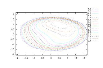
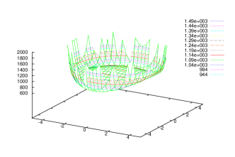
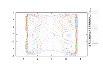
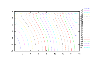
Refer to caption
(a) Contour Levels of ฮ ฮ \Pi.
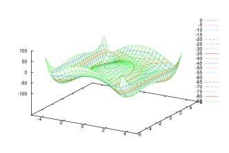
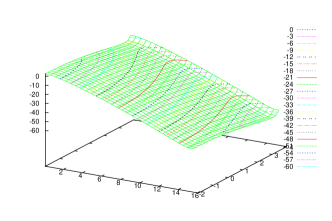
Refer to caption
(b) Graph of ฮ ฮ \Pi.
Figure 1. ฮ ฮ \Pi function of Example 1

It can be shown that ฮ dsuperscriptฮ ๐‘‘\Pi^{d} has only one critical point in ๐’ฎa+superscriptsubscript๐’ฎ๐‘Ž{\cal S}_{a}^{+} and it is given (approximately) by

๐‡ยฏ=(1.171057661103504,โˆ’0.34599084656216).ยฏ๐‡1.1710576611035040.34599084656216\overline{\mbox{\boldmath$\varsigma$}}=(1.171057661103504,-0.34599084656216).

By the triality theory, the vector

๐ฑยฏ=๐†โ€‹(๐‡ยฏ)โˆ’1โ€‹๐Ÿ=(0.54792514555217,1.003890602479819)ยฏ๐ฑ๐†superscriptยฏ๐‡1๐Ÿ0.547925145552171.003890602479819\overline{{\bf x}}={\bf G}(\overline{\mbox{\boldmath$\varsigma$}})^{-1}{\bf f}=(0.54792514555217,1.003890602479819)

is the only global minimizer of the primal problem.

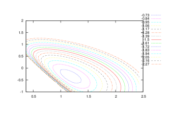
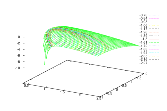
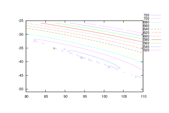
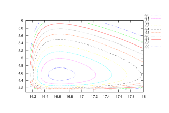
Refer to caption
(a) Contour Levels of ฮ dsuperscriptฮ ๐‘‘\Pi^{d}.
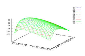
Refer to caption
(b) Graph of ฮ dsuperscriptฮ ๐‘‘\Pi^{d}.
Figure 2. ฮ dsuperscriptฮ ๐‘‘\Pi^{d} function of Example 1

4.2. One stationary point in ๐’ฎa+superscriptsubscript๐’ฎ๐‘Ž{\cal S}_{a}^{+} and one in ๐’ฎaโˆ’superscriptsubscript๐’ฎ๐‘Ž{\cal S}_{a}^{-}

Let ฮฑ1=1,ฮธ1=50formulae-sequencesubscript๐›ผ11subscript๐œƒ150\alpha_{1}=1,\;\;\theta_{1}=50, and

๐€=[100โˆ’16],๐1=[1001],๐‚1=[1002],๐Ÿ=[โˆ’259].formulae-sequence๐€delimited-[]10016formulae-sequencesubscript๐1delimited-[]1001formulae-sequencesubscript๐‚1delimited-[]1002๐Ÿdelimited-[]259{\bf A}=\left[\begin{array}[]{cc}1&0\\ 0&-16\end{array}\right],{\bf B}_{1}=\left[\begin{array}[]{cc}1&0\\ 0&1\end{array}\right],{\bf C}_{1}=\left[\begin{array}[]{cc}1&0\\ 0&2\end{array}\right],{\bf f}=\left[\begin{array}[]{c}-25\\ 9\end{array}\right].

The primal function ฮ :โ„2โ†’โ„:ฮ โ†’superscriptโ„2โ„\Pi:{\mathbb{R}}^{2}\rightarrow{\mathbb{R}} is then given by

ฮ โ€‹(x,y)=expโก(12โ€‹(x2+y2)โˆ’1)+12โ€‹(12โ€‹(x2+2โ€‹y2)โˆ’50)2+12โ€‹(x2โˆ’16โ€‹y2)+25โ€‹xโˆ’9โ€‹yฮ ๐‘ฅ๐‘ฆ12superscript๐‘ฅ2superscript๐‘ฆ2112superscript12superscript๐‘ฅ22superscript๐‘ฆ250212superscript๐‘ฅ216superscript๐‘ฆ225๐‘ฅ9๐‘ฆ\Pi(x,y)=\exp\left(\frac{1}{2}(x^{2}+y^{2})-1\right)+\frac{1}{2}\left(\frac{1}{2}(x^{2}+2y^{2})-50\right)^{2}+\frac{1}{2}(x^{2}-16y^{2})+25x-9y

and its canonical dual is

ฮ dโ€‹(ฯ„,ฯƒ)=โˆ’12โ€‹(81โˆ’16+ฯ„+2โ€‹ฯƒ+6251+ฯ„+ฯƒ)โˆ’ฯ„โ‹…lnโก(ฯ„)โˆ’12โ€‹ฯƒ2โˆ’50โ€‹ฯƒ,superscriptฮ ๐‘‘๐œ๐œŽ128116๐œ2๐œŽ6251๐œ๐œŽโ‹…๐œ๐œ12superscript๐œŽ250๐œŽ\Pi^{d}(\tau,{\sigma})=-\frac{1}{2}\left(\frac{81}{-16+\tau+2{\sigma}}+\frac{625}{1+\tau+{\sigma}}\right)-\tau\cdot\ln(\tau)-\frac{1}{2}{\sigma}^{2}-50{\sigma},

which has two critical points:

๐‡1ยฏ=(96.61711963278241,โˆ’38.94928057661689)โˆˆ๐’ฎa+,ยฏsubscript๐‡196.6171196327824138.94928057661689superscriptsubscript๐’ฎ๐‘Ž\overline{\mbox{\boldmath$\varsigma$}_{1}}=(96.61711963278241,-38.94928057661689)\in{\cal S}_{a}^{+},
๐‡2ยฏ=(0.42157060067968,โˆ’49.86072154366873)โˆˆ๐’ฎaโˆ’.ยฏsubscript๐‡20.4215706006796849.86072154366873subscriptsuperscript๐’ฎ๐‘Ž\overline{\mbox{\boldmath$\varsigma$}_{2}}=(0.42157060067968,-49.86072154366873)\in{\cal S}^{-}_{a}.

Therefore, by the triality theory, the associated vector

๐ฑ1ยฏ=๐†โ€‹(๐‡1ยฏ)โˆ’1โ€‹๐Ÿ=(โˆ’0.42612784793499,3.310578038951848)ยฏsubscript๐ฑ1๐†superscriptยฏsubscript๐‡11๐Ÿ0.426127847934993.310578038951848\overline{{\bf x}_{1}}={\bf G}(\overline{\mbox{\boldmath$\varsigma$}_{1}})^{-1}{\bf f}=(-0.42612784793499,3.310578038951848)

is the only global minimizer of ฮ โ€‹(๐ฑ)ฮ ๐ฑ\Pi({\bf x}) and

๐ฑ2ยฏ=(0.51611144112381,โˆ’0.078057328303129)ยฏsubscript๐ฑ20.516111441123810.078057328303129\overline{{\bf x}_{2}}=(0.51611144112381,-0.078057328303129)

is a local maximizer (see Figure 3) since ๐‡2ยฏยฏsubscript๐‡2\overline{\mbox{\boldmath$\varsigma$}_{2}} is a local maximum of ฮ dsuperscriptฮ ๐‘‘\Pi^{d} in ๐’ฎaโˆ’superscriptsubscript๐’ฎ๐‘Ž{\cal S}_{a}^{-} (see Figure 5).

Refer to caption
(a) Contour Levels of ฮ ฮ \Pi.
Refer to caption
(b) Graph of ฮ ฮ \Pi.
Figure 3. Primal function ฮ ฮ \Pi in Example 2
Refer to caption
(a) Contour Levels of ฮ dsuperscriptฮ ๐‘‘\Pi^{d} in ๐’ฎa+superscriptsubscript๐’ฎ๐‘Ž{\cal S}_{a}^{+}.
Refer to caption
(b) Graph of ฮ dsuperscriptฮ ๐‘‘\Pi^{d} in ๐’ฎa+superscriptsubscript๐’ฎ๐‘Ž{\cal S}_{a}^{+}.
Figure 4. ฮ dsuperscriptฮ ๐‘‘\Pi^{d} function in ๐’ฎa+superscriptsubscript๐’ฎ๐‘Ž{\cal S}_{a}^{+} of Example 2
Refer to caption
(a) Contour Levels of ฮ dsuperscriptฮ ๐‘‘\Pi^{d} in ๐’ฎaโˆ’superscriptsubscript๐’ฎ๐‘Ž{\cal S}_{a}^{-}.
Refer to caption
(b) Graph of ฮ dsuperscriptฮ ๐‘‘\Pi^{d} in ๐’ฎaโˆ’superscriptsubscript๐’ฎ๐‘Ž{\cal S}_{a}^{-}.
Figure 5. ฮ dsuperscriptฮ ๐‘‘\Pi^{d} function in ๐’ฎaโˆ’superscriptsubscript๐’ฎ๐‘Ž{\cal S}_{a}^{-} of Example 2

4.3. One stationary point in ๐’ฎa+superscriptsubscript๐’ฎ๐‘Ž{\cal S}_{a}^{+} and two in ๐’ฎaโˆ’superscriptsubscript๐’ฎ๐‘Ž{\cal S}_{a}^{-}

In order to illustrate the triality theory, we let ฮฑ1=ฮธ1=2subscript๐›ผ1subscript๐œƒ12\alpha_{1}=\theta_{1}=2, and

๐€=[โˆ’1600โˆ’4],๐1=[1000],๐‚1=[0001],๐Ÿ=[22].formulae-sequence๐€delimited-[]16004formulae-sequencesubscript๐1delimited-[]1000formulae-sequencesubscript๐‚1delimited-[]0001๐Ÿdelimited-[]22{\bf A}=\left[\begin{array}[]{cc}-16&0\\ 0&-4\end{array}\right],{\bf B}_{1}=\left[\begin{array}[]{cc}1&0\\ 0&0\end{array}\right],{\bf C}_{1}=\left[\begin{array}[]{cc}0&0\\ 0&1\end{array}\right],{\bf f}=\left[\begin{array}[]{c}2\\ 2\end{array}\right].

Accordingly, we have

ฮ โ€‹(x,y)=expโก(12โ€‹x2โˆ’2)+12โ€‹(12โ€‹y2โˆ’2)2+12โ€‹(โˆ’16โ€‹x2โˆ’4โ€‹y2)โˆ’2โ€‹xโˆ’2โ€‹y,ฮ ๐‘ฅ๐‘ฆ12superscript๐‘ฅ2212superscript12superscript๐‘ฆ2221216superscript๐‘ฅ24superscript๐‘ฆ22๐‘ฅ2๐‘ฆ\Pi(x,y)=\exp\left(\frac{1}{2}x^{2}-2\right)+\frac{1}{2}\left(\frac{1}{2}y^{2}-2\right)^{2}+\frac{1}{2}(-16x^{2}-4y^{2})-2x-2y,
ฮ dโ€‹(ฯ„,ฯƒ)=โˆ’12โ€‹(4ฯƒโˆ’4+4ฯ„โˆ’16)โˆ’ฯ„โ‹…lnโก(ฯ„)โˆ’ฯ„โˆ’12โ€‹ฯƒ2โˆ’2โ€‹ฯƒ.superscriptฮ ๐‘‘๐œ๐œŽ124๐œŽ44๐œ16โ‹…๐œ๐œ๐œ12superscript๐œŽ22๐œŽ\Pi^{d}(\tau,{\sigma})=-\frac{1}{2}\left(\frac{4}{{\sigma}-4}+\frac{4}{\tau-16}\right)-\tau\cdot\ln(\tau)-\tau-\frac{1}{2}{\sigma}^{2}-2{\sigma}.
Refer to caption
(a) Contour Levels of ฮ ฮ \Pi.
Refer to caption
(b) Graph of ฮ ฮ \Pi.
Figure 6. ฮ ฮ \Pi function of Example 3

In this case, ฮ dsuperscriptฮ ๐‘‘\Pi^{d} has in total six critical points but only one

๐‡1ยฏ=(16.64468576727409,4.552474610531074)โˆˆ๐’ฎa+,ยฏsubscript๐‡116.644685767274094.552474610531074superscriptsubscript๐’ฎ๐‘Ž\overline{\mbox{\boldmath$\varsigma$}_{1}}=(16.64468576727409,4.552474610531074)\in{\cal S}_{a}^{+},

(see Figure 7) and two

๐‡2ยฏ=(0.13641513779858,โˆ’1.943380912562619)โˆˆ๐’ฎaโˆ’,ยฏsubscript๐‡20.136415137798581.943380912562619subscriptsuperscript๐’ฎ๐‘Ž\overline{\mbox{\boldmath$\varsigma$}_{2}}=(0.13641513779858,-1.943380912562619)\in{\cal S}^{-}_{a},
๐‡3ยฏ=(15.34981976568548,3.390906302031545)โˆˆ๐’ฎaโˆ’.ยฏsubscript๐‡315.349819765685483.390906302031545subscriptsuperscript๐’ฎ๐‘Ž\overline{\mbox{\boldmath$\varsigma$}_{3}}=(15.34981976568548,3.390906302031545)\in{\cal S}^{-}_{a}.

From Figures 8 we can see that ๐‡2ยฏยฏsubscript๐‡2\overline{\mbox{\boldmath$\varsigma$}_{2}} is a local maximizer and ๐‡3ยฏยฏsubscript๐‡3\overline{\mbox{\boldmath$\varsigma$}_{3}} is a local minimizer of ฮ dsuperscriptฮ ๐‘‘\Pi^{d}. Therefore, by the triality theory, we know that

๐ฑ1ยฏ=๐†โ€‹(๐‡1ยฏ)โˆ’1โ€‹๐Ÿ=(3.102286573591542,3.620075858467906)ยฏsubscript๐ฑ1๐†superscriptยฏsubscript๐‡11๐Ÿ3.1022865735915423.620075858467906\overline{{\bf x}_{1}}={\bf G}(\overline{\mbox{\boldmath$\varsigma$}_{1}})^{-1}{\bf f}=(3.102286573591542,3.620075858467906)

is the only global minimizer;

๐ฑ2ยฏ=(โˆ’0.12607490787063,โˆ’0.33650880356205)ยฏsubscript๐ฑ20.126074907870630.33650880356205\overline{{\bf x}_{2}}=(-0.12607490787063,-0.33650880356205)

is a local maximizer and

๐ฑ3ยฏ=(โˆ’3.076070133243102,โˆ’3.283567054905852)ยฏsubscript๐ฑ33.0760701332431023.283567054905852\overline{{\bf x}_{3}}=(-3.076070133243102,-3.283567054905852)

is a local minimizer of ฮ โ€‹(๐ฑ)ฮ ๐ฑ\Pi({\bf x}) (see Figure 6).

Refer to caption
(a) Contour Levels of ฮ dsuperscriptฮ ๐‘‘\Pi^{d} in ๐’ฎa+superscriptsubscript๐’ฎ๐‘Ž{\cal S}_{a}^{+}.
Refer to caption
(b) Graph of ฮ dsuperscriptฮ ๐‘‘\Pi^{d} in ๐’ฎa+superscriptsubscript๐’ฎ๐‘Ž{\cal S}_{a}^{+}.
Figure 7. ฮ dsuperscriptฮ ๐‘‘\Pi^{d} function in ๐’ฎa+superscriptsubscript๐’ฎ๐‘Ž{\cal S}_{a}^{+} of Example 3
Refer to caption
(a) Contour Levels of ฮ dsuperscriptฮ ๐‘‘\Pi^{d} in ๐’ฎaโˆ’superscriptsubscript๐’ฎ๐‘Ž{\cal S}_{a}^{-}.
Refer to caption
(b) Graph of ฮ dsuperscriptฮ ๐‘‘\Pi^{d} in ๐’ฎaโˆ’superscriptsubscript๐’ฎ๐‘Ž{\cal S}_{a}^{-}.
Figure 8. ฮ dsuperscriptฮ ๐‘‘\Pi^{d} function in ๐’ฎaโˆ’superscriptsubscript๐’ฎ๐‘Ž{\cal S}_{a}^{-} of Example 3

4.4. Non-unique global minima

In the case that no stationary point can be found in ๐’ฎa+subscriptsuperscript๐’ฎ๐‘Ž{\cal S}^{+}_{a}, the primal problem could have more than one global minima. To see this, we let ๐Ÿโ‰ก0,ฮฑ1=ฮธ1=2formulae-sequence๐Ÿ0subscript๐›ผ1subscript๐œƒ12{\bf f}\equiv 0,\;\alpha_{1}=\theta_{1}=2, and

๐€โ‰ก0,๐1=[1000],๐‚1=[0001].formulae-sequence๐€0formulae-sequencesubscript๐1delimited-[]1000subscript๐‚1delimited-[]0001{\bf A}\equiv 0,{\bf B}_{1}=\left[\begin{array}[]{cc}1&0\\ 0&0\end{array}\right],{\bf C}_{1}=\left[\begin{array}[]{cc}0&0\\ 0&1\end{array}\right].

In this case, the primal function

ฮ โ€‹(x,y)=expโก(12โ€‹x2โˆ’2)+12โ€‹(12โ€‹y2โˆ’2)2ฮ ๐‘ฅ๐‘ฆ12superscript๐‘ฅ2212superscript12superscript๐‘ฆ222\Pi(x,y)=\exp\left(\frac{1}{2}x^{2}-2\right)+\frac{1}{2}\left(\frac{1}{2}y^{2}-2\right)^{2}

has 2 global minimums at (0,โˆ’2)02(0,-2), (0,2)02(0,2) and a local maximum at (0,0)00(0,0). While the dual function

ฮ dโ€‹(ฯ„,ฯƒ)=โˆ’ฯ„โ€‹lnโกฯ„โˆ’ฯ„โˆ’12โ€‹ฯƒ2โˆ’2โ€‹ฯƒsuperscriptฮ ๐‘‘๐œ๐œŽ๐œ๐œ๐œ12superscript๐œŽ22๐œŽ\Pi^{d}(\tau,{\sigma})=-\tau\ln\tau-\tau-\frac{1}{2}{\sigma}^{2}-2{\sigma}

does not have a stationary point in ๐’ฎa+superscriptsubscript๐’ฎ๐‘Ž{\cal S}_{a}^{+}. There is however a critical point in the boundary of ๐’ฎa+superscriptsubscript๐’ฎ๐‘Ž{\cal S}_{a}^{+}, namely, ๐‡ยฏ=(expโก(โˆ’2),0)ยฏ๐‡20\overline{\mbox{\boldmath$\varsigma$}}=(\exp(-2),0). By defining ๐ฑยฏ=๐†โ€‹(๐‡ยฏ)โˆ’1โ€‹๐Ÿยฏ๐ฑ๐†superscriptยฏ๐‡1๐Ÿ\overline{{\bf x}}={\bf G}(\overline{\mbox{\boldmath$\varsigma$}})^{-1}{\bf f}, we have that ๐ฑยฏ=(0,0)ยฏ๐ฑ00\overline{{\bf x}}=(0,0).

In order to find a global minimum of ฮ ฮ \Pi, we need to introduce the following perturbations:

๐€n=[โˆ’16n00โˆ’4n]โ€‹ย andย โ€‹๐Ÿ๐ง=[2n2n],ย for everyย โ€‹nโˆˆIโ€‹N.formulae-sequencesubscript๐€๐‘›delimited-[]16๐‘›004๐‘›ย andย subscript๐Ÿ๐งdelimited-[]2๐‘›2๐‘›ย for everyย ๐‘›๐ผ๐‘{\bf A}_{n}=\left[\begin{array}[]{cc}-\frac{16}{n}&0\\ 0&-\frac{4}{n}\end{array}\right]\text{ and }{\bf f_{n}}=\left[\begin{array}[]{c}\frac{2}{n}\\ \frac{2}{n}\end{array}\right],\text{ for every }n\in I\!\!N.

Then, the associated primal and dual functions are

ฮ nโ€‹(x,y)=expโก(12โ€‹x2โˆ’2)+12โ€‹(12โ€‹y2โˆ’2)2+12โ€‹(โˆ’16nโ€‹x2โˆ’4nโ€‹y2)โˆ’2nโ€‹xโˆ’2nโ€‹y,subscriptฮ ๐‘›๐‘ฅ๐‘ฆ12superscript๐‘ฅ2212superscript12superscript๐‘ฆ2221216๐‘›superscript๐‘ฅ24๐‘›superscript๐‘ฆ22๐‘›๐‘ฅ2๐‘›๐‘ฆ\Pi_{n}(x,y)=\exp\left(\frac{1}{2}x^{2}-2\right)+\frac{1}{2}\left(\frac{1}{2}y^{2}-2\right)^{2}+\frac{1}{2}\left(-\frac{16}{n}x^{2}-\frac{4}{n}y^{2}\right)-\frac{2}{n}x-\frac{2}{n}y,
ฮ ndโ€‹(ฯ„,ฯƒ)=โˆ’12โ€‹(4n2โ€‹(ฯ„โˆ’16n)+4n2โ€‹(ฯƒโˆ’4n))โˆ’ฯ„โ€‹lnโกฯ„+ฯ„โˆ’12โ€‹ฯƒ2โˆ’2โ€‹ฯ„โˆ’2โ€‹ฯƒ.subscriptsuperscriptฮ ๐‘‘๐‘›๐œ๐œŽ124superscript๐‘›2๐œ16๐‘›4superscript๐‘›2๐œŽ4๐‘›๐œ๐œ๐œ12superscript๐œŽ22๐œ2๐œŽ\Pi^{d}_{n}(\tau,{\sigma})=-\frac{1}{2}\left(\frac{4}{n^{2}\left(\tau-\frac{16}{n}\right)}+\frac{4}{n^{2}\left({\sigma}-\frac{4}{n}\right)}\right)-\tau\ln\tau+\tau-\frac{1}{2}{\sigma}^{2}-2\tau-2{\sigma}.

Notice that if n=1๐‘›1n=1 we are in the case presented in Example 3. Let us show that for sufficiently large values of n๐‘›n we can find a stationary point for ฮ ndsubscriptsuperscriptฮ ๐‘‘๐‘›\Pi^{d}_{n} in ๐’ฎa+superscriptsubscript๐’ฎ๐‘Ž{\cal S}_{a}^{+}, namely ๐‡nยฏยฏsubscript๐‡๐‘›\overline{\mbox{\boldmath$\varsigma$}_{n}}. Furthermore, by defining ๐ฑยฏn=๐†โ€‹(๐‡ยฏn)โˆ’1โ€‹๐Ÿ๐งsubscriptยฏ๐ฑ๐‘›๐†superscriptsubscriptยฏ๐‡๐‘›1subscript๐Ÿ๐ง\overline{{\bf x}}_{n}={\bf G}(\overline{\mbox{\boldmath$\varsigma$}}_{n})^{-1}{\bf f_{n}} we will have a convergent sequence.

Let us calculate the gradient of ฮ ndsubscriptsuperscriptฮ ๐‘‘๐‘›\Pi^{d}_{n}:

โˆ‡ฮ ndโ€‹(ฯ„,ฯƒ)=[โˆ’2โˆ’lnโกฯ„+2(nโ€‹ฯ„โˆ’16)2โˆ’ฯƒโˆ’2+2(nโ€‹ฯƒโˆ’4)2].โˆ‡subscriptsuperscriptฮ ๐‘‘๐‘›๐œ๐œŽdelimited-[]2๐œ2superscript๐‘›๐œ162๐œŽ22superscript๐‘›๐œŽ42{\bf\nabla}\Pi^{d}_{n}(\tau,{\sigma})=\left[\begin{array}[]{c}-2-\ln\tau+\frac{2}{(n\tau-16)^{2}}\\ -{\sigma}-2+\frac{2}{(n{\sigma}-4)^{2}}\end{array}\right].

Let hโ€‹(ฯ„)=โˆ’2โˆ’lnโกฯ„+2(nโ€‹ฯ„โˆ’16)2โ„Ž๐œ2๐œ2superscript๐‘›๐œ162h(\tau)=-2-\ln\tau+\frac{2}{(n\tau-16)^{2}} and gโ€‹(ฯƒ)=โˆ’ฯƒโˆ’2+2(nโ€‹ฯƒโˆ’4)2๐‘”๐œŽ๐œŽ22superscript๐‘›๐œŽ42g({\sigma})=-{\sigma}-2+\frac{2}{(n{\sigma}-4)^{2}}. It is not difficult to show that there exists a sufficiently large NโˆˆIโ€‹N๐‘๐ผ๐‘N\in I\!\!N, such that if n>N๐‘›๐‘n>N, the following are true:

  1. a)

    nโ‹…expโก(โˆ’2+1n)โˆ’16โ€‹ย andย โ€‹nโ‹…expโก(โˆ’2)โˆ’16โ‹…๐‘›21๐‘›โ‹…16ย andย ๐‘›216\displaystyle n\cdot\exp\left(-2+\frac{1}{n}\right)-16\text{ and }n\cdot\exp\left(-2\right)-16 are positive numbers.

  2. b)

    hโ€‹(expโก(โˆ’2+1n))=2(nโ‹…expโก(โˆ’2+1n)โˆ’16)2โˆ’1n<0<hโ€‹(expโก(โˆ’2))=2(nโ‹…expโก(โˆ’2)โˆ’16)2โ„Ž21๐‘›2superscriptโ‹…๐‘›21๐‘›1621๐‘›0โ„Ž22superscriptโ‹…๐‘›2162\displaystyle h\left(\exp\left(-2+\frac{1}{n}\right)\right)=\frac{2}{(n\cdot\exp(-2+\frac{1}{n})-16)^{2}}-\frac{1}{n}\\ <0<h(\exp(-2))=\frac{2}{(n\cdot\exp(-2)-16)^{2}}.

  3. c)

    gโ€‹(5.1n)โ‰ˆโˆ’5.1nโˆ’0.34710743801<0<gโ€‹(4.9n)โ‰ˆ0.46913580247โˆ’4.9n.๐‘”5.1๐‘›5.1๐‘›0.347107438010๐‘”4.9๐‘›0.469135802474.9๐‘›\displaystyle g\left(\frac{5.1}{n}\right)\approx-\frac{5.1}{n}-0.34710743801<0<g\left(\frac{4.9}{n}\right)\approx 0.46913580247-\frac{4.9}{n}.

Based on these results, we know that for every n>N๐‘›๐‘n>N, โˆ‡ฮ ndโˆ‡subscriptsuperscriptฮ ๐‘‘๐‘›{\bf\nabla}\Pi^{d}_{n} has a stationary point ๐‡ยฏn=(ฯ„ยฏn,ฯƒยฏn)โˆˆsubscriptยฏ๐‡๐‘›subscriptยฏ๐œ๐‘›subscriptยฏ๐œŽ๐‘›absent\overline{\mbox{\boldmath$\varsigma$}}_{n}=(\overline{\tau}_{n},\overline{{\sigma}}_{n})\in [expโก(โˆ’2),expโก(โˆ’2+1n)]ร—[4.9n,5.1n]221๐‘›4.9๐‘›5.1๐‘›[\exp(-2),\exp(-2+\frac{1}{n})]\times\left[\frac{4.9}{n},\frac{5.1}{n}\right]. Moreover, by the fact that gโ€‹(ฯƒยฏn)=0๐‘”subscriptยฏ๐œŽ๐‘›0g(\overline{{\sigma}}_{n})=0, it is easy to obtain limnโ†’+โˆžnโ‹…ฯƒยฏn=5subscriptโ†’๐‘›โ‹…๐‘›subscriptยฏ๐œŽ๐‘›5\displaystyle\lim_{n\rightarrow+\infty}n\cdot\overline{{\sigma}}_{n}=5.

Notice also that

๐†โ€‹(๐‡ยฏn)=[ฯ„ยฏnโˆ’16n00ฯƒยฏnโˆ’4n]๐†subscriptยฏ๐‡๐‘›delimited-[]subscriptยฏ๐œ๐‘›16๐‘›00subscriptยฏ๐œŽ๐‘›4๐‘›{\bf G}(\overline{\mbox{\boldmath$\varsigma$}}_{n})=\left[\begin{array}[]{cc}\displaystyle\overline{\tau}_{n}-\frac{16}{n}&0\\ 0&\overline{{\sigma}}_{n}-\frac{4}{n}\end{array}\right]

is positive definite. Therefore, the perturbed solution can be obtained as

๐ฑยฏn=๐†โ€‹(๐‡ยฏn)โˆ’1โ€‹๐Ÿ๐ง=[2nโ‹…ฯ„ยฏnโˆ’162nโ‹…ฯƒยฏnโˆ’4].subscriptยฏ๐ฑ๐‘›๐†superscriptsubscriptยฏ๐‡๐‘›1subscript๐Ÿ๐งdelimited-[]2โ‹…๐‘›subscriptยฏ๐œ๐‘›162โ‹…๐‘›subscriptยฏ๐œŽ๐‘›4\overline{{\bf x}}_{n}={\bf G}(\overline{\mbox{\boldmath$\varsigma$}}_{n})^{-1}{\bf f_{n}}=\left[\begin{array}[]{c}\frac{2}{n\cdot\overline{\tau}_{n}-16}\\ \frac{2}{n\cdot\overline{{\sigma}}_{n}-4}\end{array}\right].

Since ฯ„ยฏnโˆˆ[expโก(โˆ’2),expโก(โˆ’2+1n)]subscriptยฏ๐œ๐‘›221๐‘›\overline{\tau}_{n}\in[\exp(-2),\exp(-2+\frac{1}{n})] then limnโ†’+โˆžฯ„n=expโก(โˆ’2)subscriptโ†’๐‘›subscript๐œ๐‘›2\displaystyle\lim_{n\rightarrow+\infty}\tau_{n}=\exp(-2). By the fact that limnโ†’+โˆžnโ‹…ฯƒยฏn=5subscriptโ†’๐‘›โ‹…๐‘›subscriptยฏ๐œŽ๐‘›5\displaystyle\lim_{n\rightarrow+\infty}n\cdot\overline{{\sigma}}_{n}=5, we have

limnโ†’+โˆž๐ฑยฏn=[02],subscriptโ†’๐‘›subscriptยฏ๐ฑ๐‘›delimited-[]02\lim_{n\rightarrow+\infty}\overline{{\bf x}}_{n}=\left[\begin{array}[]{c}0\\ 2\end{array}\right],

which is a solution of ฮ ฮ \Pi.

Canonical perturbation method was originally introduced in [31] for solving nonconvex polynomial minimization problems. This method has been used successfully in integer programming and network communication (see [17, 37]).

5. Future Research

Some open questions that will be studied in the future are the following:

  1. โˆ™โˆ™\bullet

    As stated in Remark 1, in order to use the canonical dual transformation a necessary condition is that (๐’ซ)๐’ซ({\cal{P}}) has a unique solution. Is this also a sufficient condition? In other words, giving (๐’ซ)๐’ซ({\cal{P}}) such that it has a unique solution, can we find a stationary point of ฮ dsuperscriptฮ ๐‘‘\Pi^{d} in ๐’ฎa+superscriptsubscript๐’ฎ๐‘Ž{\cal S}_{a}^{+}?

  2. โˆ™โˆ™\bullet

    Example 4 shows an interesting perturbation method that allows us to solve a problem when the necessary condition of Remark 1 is not satisfied. Can we generalize this method and develop an algorithm?

6. Appendix: Some Lemmas in Matrix Analysis

The following results are needed in the proofs of Section 2.

Lemma 3.

(Singular value decomposition [22]) For any given matrix ๐ŒโŠ‚โ„mร—n๐Œsuperscriptโ„๐‘š๐‘›{\bf M}\subset{\mathbb{R}}^{m\times n} with Rankย โ€‹(๐Œ)=rRankย ๐Œ๐‘Ÿ{\mbox{Rank }}({\bf M})=r, there exists ๐”โŠ‚โ„mร—m๐”superscriptโ„๐‘š๐‘š{\bf U}\subset{\mathbb{R}}^{m\times m}, ๐‘โŠ‚โ„mร—n๐‘superscriptโ„๐‘š๐‘›{\bf R}\subset{\mathbb{R}}^{m\times n} and ๐„โŠ‚โ„nร—n๐„superscriptโ„๐‘›๐‘›{\bf E}\subset{\mathbb{R}}^{n\times n} such that

๐Œ=๐”๐‘๐„;๐Œ๐”๐‘๐„{\bf M}={\bf U}{\bf R}{\bf E};

where ๐”๐”{\bf U} and ๐„๐„{\bf E} are orthogonal matrices, and

Riโ€‹j={si,i=j,i=1,โ€ฆ,r0,iโ‰ j,subscript๐‘…๐‘–๐‘—casessubscript๐‘ ๐‘–formulae-sequence๐‘–๐‘—๐‘–1โ€ฆ๐‘Ÿ0๐‘–๐‘—R_{ij}=\left\{\begin{array}[]{ll}s_{i},&i=j,\ i=1,\ldots,r\\ 0,&i\neq j,\end{array}\right.

where si>0subscript๐‘ ๐‘–0s_{i}>0 for every i=1,โ€ฆ,r๐‘–1โ€ฆ๐‘Ÿi=1,\ldots,r.

Lemma 4.

[22] If ๐†๐†{\bf G} and ๐”๐”{\bf U} are positive definite matrices in โ„nร—nsuperscriptโ„๐‘›๐‘›{\mathbb{R}}^{n\times n}, then ๐†โชฐ๐”succeeds-or-equals๐†๐”{\bf G}\succeq{\bf U} if and only if ๐”โˆ’1โชฐ๐†โˆ’1succeeds-or-equalssuperscript๐”1superscript๐†1{\bf U}^{-1}\succeq{\bf G}^{-1}.

Lemma 5.

[20] Suppose ๐๐{\bf P}, ๐”๐”{\bf U} and ๐ƒ๐ƒ{\bf D} are three matrices in โ„nร—nsuperscriptโ„๐‘›๐‘›{\mathbb{R}}^{n\times n} such that

๐ƒ=[๐ƒ110mร—(nโˆ’m)0(nโˆ’m)ร—n0(nโˆ’m)ร—(nโˆ’m)],๐ƒdelimited-[]subscript๐ƒ11subscript0๐‘š๐‘›๐‘šsubscript0๐‘›๐‘š๐‘›subscript0๐‘›๐‘š๐‘›๐‘š{\bf D}=\left[\begin{array}[]{cc}{\bf D}_{11}&0_{m\times(n-m)}\\ 0_{(n-m)\times n}&0_{(n-m)\times(n-m)}\end{array}\right],

where ๐ƒ11โˆˆโ„mร—msubscript๐ƒ11superscriptโ„๐‘š๐‘š{\bf D}_{11}\in{\mathbb{R}}^{m\times m} is nonsingular and

๐=[๐11๐12๐21๐22]โ‰บ0,๐”=[๐”110mร—(nโˆ’m)0(nโˆ’m)ร—m๐”22]โ‰ป0,formulae-sequence๐delimited-[]subscript๐11subscript๐12subscript๐21subscript๐22precedes0๐”delimited-[]subscript๐”11subscript0๐‘š๐‘›๐‘šsubscript0๐‘›๐‘š๐‘šsubscript๐”22succeeds0{\bf P}=\left[\begin{array}[]{cc}{\bf P}_{11}&{\bf P}_{12}\\ {\bf P}_{21}&{\bf P}_{22}\end{array}\right]\prec 0,\ {\bf U}=\left[\begin{array}[]{cc}{\bf U}_{11}&0_{m\times(n-m)}\\ 0_{(n-m)\times m}&{\bf U}_{22}\end{array}\right]\succ 0,

๐iโ€‹jsubscript๐๐‘–๐‘—{\bf P}_{ij} and ๐”iโ€‹isubscript๐”๐‘–๐‘–{\bf U}_{ii} are appropriate dimensional matrices for i,j=1,2formulae-sequence๐‘–๐‘—12i,j=1,2. Then,

(47) ๐+๐ƒ๐”๐ƒtโชฏ0โŸบโˆ’๐ƒtโ€‹๐โˆ’1โ€‹๐ƒโˆ’๐”โˆ’1โชฏ0.โŸบprecedes-or-equals๐superscript๐ƒ๐”๐ƒ๐‘ก0precedes-or-equalssuperscript๐ƒ๐‘กsuperscript๐1๐ƒsuperscript๐”10{\bf P}+{\bf D}{\bf U}{\bf D}^{t}\preceq 0\Longleftrightarrow-{\bf D}^{t}{\bf P}^{-1}{\bf D}-{\bf U}^{-1}\preceq 0.

โ€…

Acknowledgements.
This research is supported by US Air Force Office of Scientific Research under the grant AFOSR FA9550-10-1-0487. Comments and suggestions from editor and reviewers are sincerely acknowledged.

References

  • [1] Aspnes, J.; Goldberg, D.; Yang, Y. R. On the computational complexity of sensor network localization. Lecture Notes in Computer Science (3121), Springer-Verlag, pp. 32-44 (2004).
  • [2] Cai, K; Gao, D. Y. and Qin, Q. H. Post-buckling solutions of hyper-elastic beam by canonical dual finite element method. To appear in Mathematics and Mechanics of Solids.
  • [3] Desoer, C. A.; Whalen, B. H. A Note on Pseudoinverses. Journal of the Society for Industrial and Applied Mathematics, Vol. 11, No 2, pp. 442-447 (1963).
  • [4] Feng, J. M.; Lin, G. X.; Sheu, R. L.; Xia, Y. Duality and solutions for quadratic programming over single non-homogeneous quadratic constraint. Journal of Global Optimization, Published online: 17 Nov 2010.
  • [5] Gao, D. Y. Dual extremum principles in finite deformation theory with applications to post-buckling analysis of extended nonlinear beam theory. Applied Mechanics Reviews, 50 (11), S64-S71 (1997).
  • [6] Gao, D. Y. Complementary finite element method for finite deformation nonsmooth mechanics. J. Eng. Math., 30, pp. 339-353 (1996).
  • [7] Gao, D. Y. Duality, triality and complementary extremum principles in nonconvex parametric variational problems with applications. IMA J. Appl. Math., 61, pp. 199-235 (1998).
  • [8] Gao, D. Y. General Analytic Solutions and Complementary Variational Principles for Large Deformation Nonsmooth Mechanics. Meccanica, 34, pp. 169-198 (1999).
  • [9] Gao, D. Y. Duality Principles in nonconvex systems. Theory Methods and Applications. Kluwer Academic Publishers, Dordrecht/Boston (2000).
  • [10] Gao, D. Y. Canonical dual transformation method and generalized triality theory in nonsmooth global optimization. J. Glob. Optim. 17(1/4), pp. 127-160 (2000).
  • [11] Gao, D. Y. Nonconvex semi-linear problems and canonical dual solutions. Advances in Mechanics and Mathematics, Kluwer Academic Publishers, Dordrecht, vol. II, pp. 261 -312 (2003).
  • [12] Gao, D.Y. Perfect duality theory and complete solutions to a class of global optimization problems. Optim., 52(4โ€“5), pp. 467-493 (2003).
  • [13] Gao, D. Y. Canonical duality theory: theory, method, and applications in global optimization. Comput. Chem. 33, pp. 1964-1972, (2009).
  • [14] Gao, D. Y.; Ogden R. W. Multiple solutions to non-convex variational problems with implications for phase transitions and numerical computation. Q. J. Mech. Appl. Math, Vol. 61. No. 4, pp. 497-522 (2008).
  • [15] Gao, D.Y; Ogden, R.W. Closed-form solutions, extremality and nonsmoothness criteria in a large deformation elasticity problem, Zeitschrift f r angewandte Mathematik und Physik (ZAMP), 59, pp.498 517 (2008).
  • [16] Gao, D. Y.; Ruan N. Solutions and optimality criteria for nonconvex quadratic-exponential minimization problem,. Math. Meth. Operations Research, 67 (3), pp. 479-491 (2008).
  • [17] Gao, D. Y., Ruan, N; Pardalos, P. M. Canonical dual solutions to sum of fourth-order polynomials minimization problems with applications to sensor network localization. Sensors: Theory, Algorithms and Applications, Springer(2010).
  • [18] Gao, D. Y.; Sherali, H. D. Canonical duality: Connection between nonconvex mechanics and global optimization. Advances in Appl. Mathematics and Global Optimization, pp. 249-316, Springer (2009).
  • [19] Gao, D. Y.; Strang, G. Geometric nonlinearity: Potential energy, complementary energy, and the gap function. Quart. Appl. Math. 47 (3), pp. 487-504 (1989).
  • [20] Gao, D. Y.; Wu, C. On the triality theory for a quartic polynomial optimization problem. J. Industrial and Management Optimization, 8(1), pp. 229-242 (2012).
  • [21] Gao, D. Y.; Yu, H. F. Multi-scale modelling and canonical dual finite element method in phase transitions of solids. Int. J. Solids and Structures, 45, pp. 3660-3673 (2008).
  • [22] Horn, R. A.; Johnson, C. R. Matrix Analysis. Cambridge University Press (1985).
  • [23] Marsden, J. E.; Hughes, T. J. R. Mathematical Foundations of Elasticity. Prentice-Hall, (1983).
  • [24] Maxima.sourceforge.net. Maxima, a Computer Algebra System. Version 5.22.1 (2010). http://maxima.sourceforge.net/
  • [25] Morรฉ, J.; Wu, Z. Global continuation for distance geometry problems. SIAM Journal on Optimization, 7, pp. 814-836 (1997).
  • [26] Moreau, J. J. La notion de sur-potentiel et les liaisons unilatรฉrales en รฉlastostatique. C.R. Acad. Sc. Paris, 267 A, pp. 954-957 (1968).
  • [27] Moreau, J. J.; Panagiotopoulos, P. D.; Strang, G. Topics in nonsmooth mechanics. Birkhuser Verlag, Basel-Boston, MA. (1988).
  • [28] Peters, G.; Wilkinson J. H. The least squares problem and pseudo-inverses. The Computer Journal, Vol. 13, No 3, pp. 309-316 (1970).
  • [29] Ruan, N.; Gao, D. Y. Canonical duality approach for non-linear dynamical systems. IMA J. Appl. Math, 79(2), 313 - 325 (2014).
  • [30] Ruan, N.; Gao, D.Y. Global optimal solutions to a general sensor network localization problem, Performance Evaluations 75-76: 1 16 (2014).
  • [31] Ruan, N.; Gao, D. Y.; Jiao, Y. Canonical dual least square method for solving general nonlinear systems of quadratic equations. Computational Optimization and Applications, Vol 47, pp. 335-347 (2010).
  • [32] Santos, H. A. F. A.; Gao D. Y. Canonical dual finite element method for solving post-buckling problems of a large deformation elastic beam. Int. J. Nonlinear Mechanics, 47, 240-247 (2012). doi:10.1016/j.ijnonlinmec.2011.05.012 (2011).
  • [33] Saxe, J. Embeddability of weighted graphs in k-space is strongly NP-hard. Proc. 17th Allerton Conference in Communications, Control, and Computing, Monticello, IL, pp. 480-489 (1979).
  • [34] Sewell, M. J. Maximum and minimum principles. Cambridge University Press, Cambridge, New York, Port Chester, Melbourne Sydney (1987).
  • [35] Strugariu, R.; Voisei, M.D.; Zalinescu, C. Counter-examples in bi-duality, triality and tri-duality, Discrete and Continuous Dynamical Systems, 31, 1453 - 1468 (2011).
  • [36] Voisei, M.D.; Zalinescu, C.: Some remarks concerning Gao-Strangโ€™s complementary gap function, Applicable Analysis, 90, 1111-1121 (2010).
  • [37] Wang, Z. B.; Fang, S. C.; Gao, D. Y.; Xing, W. X. Canonical dual approach to solving the maximum cut problem. J. Glob. Optim., 54, 341โ€“352 (2012).
  • [38] Xie D.; Schlick T. Visualization of chemical databases using the singular value decomposition and truncated-Newton minimization. Optimization in Computational Chemistry and Molecular Biology, Kluwer Academic Publishers B.V. (2000).
  • [39] Zhang J.; Gao, D. Y.; Yearwood, J. A novel canonical dual computational approach for prion AGAAAAGA amyloid fibril molecular modeling. Journal of Theoretical Biology, 284, pp. 149-157 (2011). doi:10.1016/j.jtbi.2011.06.024
  • [40] Zia, R. K. P.; Redish, E. F.; McKay S. R. Making Sense of the Legendre Transform American Journal of Physics, Vol. 77, Issue 7, pp. 614-622 (2009).