Decoding a Class of Affine Variety Codes
with Fast DFT

Abstract

An efficient procedure for error-value calculations based on fast discrete Fourier transforms (DFT) in conjunction with Berlekamp-Massey-Sakata algorithm for a class of affine variety codes is proposed. Our procedure is achieved by multidimensional DFT and linear recurrence relations from Grobner basis and is applied to erasure-and-error decoding and systematic encoding. The computational complexity of error-value calculations in our algorithm improves that in solving systems of linear equations from error correcting pairs for many cases. A motivating example of our algorithm in case of Reed-Solomon codes and a numerical example of our algorithm in case of a Hermitian code are also described.

I Introduction

Affine variety codes [5],[10] are the generalization of algebraic geometry (AG) codes and they are defined by a pair of a monomial order and any subset of $\mathbb{F}_{q}^{N}$, where $\mathbb{F}_{q}$ is the finite field of $q$-elements and $N$ is a positive integer. It is known [5] that affine variety codes represent all linear codes.

The fast decoding of affine variety codes can be divided into two steps, namely error-location step and error-evaluation step. As for the fast error-location step, it is shown [2],[4] that Berlekamp–Massey–Sakata (BMS) algorithm finding the Gröbner basis of error-locator ideals for AG codes is generalized to that for affine variety codes. As for the fast error-evaluation step, it is shown [7] that Forney’s method is generalized to affine variety codes. On the other hand, in [9], the author showed another fast error-evaluation method based on multidimensional DFT and linear recurrence relations from Gröbner basis of error-locator ideals. The method in [9] is the generalization of the results in [13],[14] for AG codes and can be applied to erasure-and-error decoding and systematic encoding of affine variety codes.

In this paper, we restrict the codes to a subclass of affine variety codes that are defined by a pair of a monomial order and any subset of $\left(\mathbb{F}_{q}^{\times}\right)^{N}$, where $\mathbb{F}_{q}^{\times}=\mathbb{F}_{q}\backslash\{0\}$, in order to apply efficiently fast DFT. This enables us to reduce the computational complexity of the error-evaluation step of [9] in their erasure-and-error decoding and systematic encoding.

The rest of this paper is organized as follows. Sec. II explains the case of Reed–Solomon codes. Sec. III describes a lemma. Subsec. III-A formulates multidimensional DFT. Subsec. III-B defines two vector spaces via Gröbner basis. Subsec. III-C defines linear recurrence relations from Gröbner basis. Subsec. III-D gives an isomorphism between the vector spaces. Sec. IV applies the lemma to a class of affine variety codes. Subsec. IV-A constructs the codes. Subsec. IV-B proposes an erasure-and-error decoding algorithm. Subsec. IV-C relates erasure-only decoding with systematic encoding. Sec. V estimates the computational complexity of our algorithm.

II A motivating example: Reed–Solomon codes

Throughout this paper, $\mathbb{N}_{0}$ is the set of non-negative integers and $\alpha$ is a fixed primitive element of finite field $\mathbb{F}_{q}$, where $q$ is a prime power. Recall the encoding of Reed–Solomon (RS) codes by polynomial division

$$c(x)=h(x)-R(x)=Q(x)G(x),\quad\deg(R)<n-k,$$ (1)

where $h(x)=\sum_{0\leq i<n}h_{i}x^{i}$ is an information polynomial with $h_{i}=0$ for $0\leq i<n-k$; $G(x)=(x-1)\cdots(x-\alpha^{n-k-1})$, the generator polynomial; $R(x)$, the remainder of the division with quotient $Q(x)$. Then $\left(c_{i}\right)_{0\leq i<n}$ from $c(x)=\sum_{0\leq i<n}c_{i}x^{i}$ is a codeword of the RS code

$$C(m)=\left\{\left(c_{i}\right)_{0\leq i<n}\in\mathbb{F}_{q}^{n}\,\left|\,c(\alpha^{i})=0\mbox{ for all }0\leq i\leq m\right.\right\}$$

with $n=q-1$ and $m=n-k-1$. This method is systematic, i.e., $c_{i}=h_{i}$ for $n-k\leq i<n$. It is well-known that a non-systematic encoding method is given by the IDFT $c_{i}=h(\alpha^{-i})=\sum_{0\leq l<n}h_{l}\alpha^{-il}$ since $\left(c_{i}\right)_{0\leq i<n}$ is another codeword of $C(m)$ by the Fourier inversion formula

$$c(\alpha^{i^{\prime}})=\sum_{0\leq l<n}h_{l}\sum_{0\leq i<n}\alpha^{i(i^{\prime}-l)}=(q-1)h_{i^{\prime}}.$$ (2)

It is possible to encode systematically by adding another procedure “extension.” From (1), we obtain $h(\alpha^{i})=R(\alpha^{i})$ for $0\leq i<n-k$. Define a vector $\left(d_{i}\right)_{0\leq i<n}$ inductively by

$$d_{i}=\left\{\begin{array}[]{ll}h(\alpha^{i})&0\leq i<n-k\\ -\sum_{l=0}^{n-k-1}G_{l}d_{l+i-(n-k)}&n-k\leq i<n,\end{array}\right.$$ (3)

where $G(x)=\sum_{l=0}^{n-k-1}G_{l}x^{l}+x^{n-k}$. Then $d_{i}=R(\alpha^{i})$ holds not only for $0\leq i<n-k$ but also for $n-k\leq i<n$; when $r$ denotes $n-k$, this fact is proved inductively by

$$d_{i}=-\sum_{l^{\prime}=0}^{r-1}R_{l^{\prime}}\alpha^{l^{\prime}(i-r)}\sum_{l=0}^{r-1}G_{l}\alpha^{l^{\prime}l}=\sum_{l^{\prime}=0}^{r-1}R_{l^{\prime}}\alpha^{l^{\prime}i},$$ (4)

where $R(x)$ is denoted by $R(x)=\sum_{l=0}^{r-1}R_{l}x^{l}$ and the last equality is deduced from $G(\alpha^{l^{\prime}})=\sum_{l=0}^{r-1}G_{l}\alpha^{l^{\prime}l}+\alpha^{l^{\prime}r}=0$ for $0\leq l^{\prime}<r$. Thus, the IDFT $\left(-d(\alpha^{-i})\right)_{0\leq i<n}$ for $d(x)=\sum_{l=0}^{n-1}d_{l}x^{l}$ agrees with $(R_{i})_{0\leq i<n}$ of $R(x)$ by using Fourier inversion formula (2); $c(x)=h(x)-R(x)$ again indicates the encoding, and moreover we obtain two ways of calculating $R(x)$, i.e., a remarkable commutative diagram.

This encoding method is applicable to decoding method. If we have received a polynomial $\overline{c}(x)=\sum_{0\leq i<n}\overline{c}_{i}x^{i}=c(x)+e(x)$ containing an error polynomial $e(x)$ in the channel, the syndrome vector $\left(e(\alpha^{i})\right)_{0\leq i<n-k}$ can be computed as $\left(\overline{c}(\alpha^{i})\right)_{0\leq i<n-k}$ by substituting the roots of $G(x)$ into $\overline{c}(x)$. Similarly to (3), we define a vector $\left(s_{i}\right)_{0\leq i<n}$ inductively by

$$s_{i}=\left\{\begin{array}[]{ll}\overline{c}(\alpha^{i})&0\leq i<n-k\\ -\sum_{l=0}^{t-1}\sigma_{l}s_{l+i-(n-k)}&n-k\leq i<n,\end{array}\right.$$ (5)

where $\sigma(x)=\sum_{l=0}^{t-1}\sigma_{l}x^{l}+x^{t}$ is the error-locator polynomial and $t\leq(n-k)/2$ is assumed. Then, it follows from the same argument as (4) that $s_{i}=e(\alpha^{i})$ with $e(x)=\sum_{l=0}^{n-1}e_{l}x^{l}$ for $0\leq i<n$. Thus, the IDFT $\left(-s(\alpha^{-i})\right)_{0\leq i<n}$ for $s(x)=\sum_{l=0}^{n-1}s_{l}x^{l}$ agrees with $(e_{i})_{0\leq i<n}$ by using Fourier inversion formula (2); $c(x)=\overline{c}(x)-e(x)$ indicates the correct codeword.

Example 1

Consider $C(3)$ of length $n=10$ and dimension $k=6$ over $\mathbb{F}_{11}=\mathrm{GF}(11)=\{0,1,2,\cdots,10\;\mathrm{mod}\,11\}$. We fix a primitive element $2$ of $\mathbb{F}_{11}$. We set information

$$\left(h_{i}\right)_{0\leq i<10}=(0,0,0,0,1,7,3,2,0,5).$$

Then we have a non-systematic codeword

$$\left(c_{i}=h(2^{-i})\right)_{0\leq i<10}=(7,10,3,5,6,1,5,1,3,3)\in C(3).$$

For systematic encoding, divide $h(x)$ by $G(x)=(x-1)(x-2)(x-4)(x-8)=9+x+4x^{2}+7x^{3}+x^{4}$ and obtain $h(x)=Q(x)G(x)+(9+2x+7x^{3})$. Thus $c(x)=h(x)-(9+2x+7x^{3})$ is a systematic codeword, where

$$\left(c_{i}\right)_{0\leq i<10}=(2,9,0,4,1,7,3,2,0,5).$$

This codeword is also computed by our method as follows.

$$\left(h(2^{i})\right)_{0\leq i<10} =(7,3,3,1,5,1,6,5,3,10)$$

$$\left(d_{i}\right)_{0\leq i<10} =(7,3,3,1,3,0,4,4,6,4)$$

$$\left(-d(2^{-i})\right)_{0\leq i<10} =(9,2,0,7,0,0,0,0,0,0)$$

$$\left(c_{i}\right)_{0\leq i<10} =(2,9,0,4,1,7,3,2,0,5)\in C(3)$$

Next, a received word can be decoded as follows.

$$\left(\overline{c}_{i}\right)_{0\leq i<10} =(1,9,0,4,1,7,3,2,0,10)$$

$$\left(\overline{c}(2^{i})\right)_{0\leq i<10} =(4,7,3,1,2,6,4,7,5,4),\,(\sigma_{l})=(6,4,1)$$

$$\left(s_{i}\right)_{0\leq i<10} =(4,7,3,1,0,5,2,6,8,9)$$

$$\left(-s(2^{-i})\right)_{0\leq i<10} =(10,0,0,0,0,0,0,0,0,5)$$

$$\left(c_{i}\right)_{0\leq i<10} =(2,9,0,4,1,7,3,2,0,5)\in C(3)\;\;\Box$$

It is shown [8] that the encoding and decoding with extension and fast DFT and IDFT actually have less computational complexity than the ordinary ones for many cases of RS codes.

III Main lemma

III-A Discrete Fourier transforms on $\left(\mathbb{F}_{q}^{\times}\right)^{N}$

Let $N$ be a positive integer and let

$$A =\left\{\underline{a}=\left(a_{1},\cdots,a_{N}\right)\left|\begin{array}[]{c}0\leq a_{i}\leq q-2\\ \mbox{for all }1\leq i\leq N\end{array}\right\}\right.,$$

$$\Omega =\left(\mathbb{F}_{q}^{\times}\right)^{N}=\left\{\left.\underline{\omega}=\left(\omega_{1},\cdots,\omega_{N}\right)\,\right|\,\omega_{1},\cdots,\omega_{N}\in\mathbb{F}_{q}^{\times}\right\},$$

where $\mathbb{F}_{q}^{\times}=\left.\mathbb{F}_{q}\right\backslash\{0\}$. Then $A$ is considered as the additive group $\left(\mathbb{Z}/(q-1)\mathbb{Z}\right)^{N}$, where $\mathbb{Z}/(q-1)\mathbb{Z}$ is the ring of integers modulo $(q-1)$. In this subsection, the discrete Fourier transforms are defined as maps between two vector spaces, which are isomorphic to $\mathbb{F}_{q}^{|A|}=\mathbb{F}_{q}^{|\Omega|}$,

$$V_{A} =\left\{\left(h_{\underline{a}}\right)_{A}\,\left|\,\underline{a}\in A,\,h_{\underline{a}}\in\mathbb{F}_{q}\right.\right\},$$

$$V_{\Omega} =\left\{\left.\left(c_{\underline{\omega}}\right)_{\Omega}\,\right|\,\underline{\omega}\in\Omega,\,c_{\underline{\omega}}\in\mathbb{F}_{q}\right\}.$$

Definition 1

For $\left(c_{\underline{\omega}}\right)_{\Omega}\in V_{\Omega}$, let $\mathcal{F}\left(\left(c_{\underline{\omega}}\right)_{\Omega}\right)\in V_{A}$ be defined as

$$\mathcal{F}\left(\left(c_{\underline{\omega}}\right)_{\Omega}\right)=\left(\sum_{\underline{\omega}\in\Omega}c_{\underline{\omega}}\underline{\omega}^{\underline{a}}\right)_{A}\in V_{A},$$ (6)

where $\underline{\omega}^{\underline{a}}=\omega_{1}^{a_{1}}\cdots\omega_{N}^{a_{N}}$. The linear map $\mathcal{F}:V_{\Omega}\to V_{A}$ of (6) is called DFT on $\left(\mathbb{F}_{q}^{\times}\right)^{N}$. Moreover, for $\left(h_{\underline{a}}\right)_{A}\in V_{A}$, let $\mathcal{F}^{-1}\left(\left(h_{\underline{a}}\right)_{A}\right)\in V_{\Omega}$ be defined as

$$\mathcal{F}^{-1}\left(\left(h_{\underline{a}}\right)_{A}\right)=\left((-1)^{N}\sum_{\underline{a}\in A}h_{\underline{a}}\underline{\omega}^{-\underline{a}}\right)_{\Omega}\in V_{\Omega}.$$ (7)

The linear map $\mathcal{F}^{-1}:V_{A}\to V_{\Omega}$ of (7) is called IDFT on $\left(\mathbb{F}_{q}^{\times}\right)^{N}$. $\Box$

Then we have Fourier inversion formulae: Two linear maps $\mathcal{F}:V_{\Omega}\to V_{A}$ and $\mathcal{F}^{-1}:V_{A}\to V_{\Omega}$ are inverse each other, i.e., $\mathcal{F}^{-1}\left(\mathcal{F}\left(\left(c_{\underline{\omega}}\right)_{\Omega}\right)\right)=\left(c_{\underline{\omega}}\right)_{\Omega}$ and $\mathcal{F}\left(\mathcal{F}^{-1}\left(\left(h_{\underline{a}}\right)_{A}\right)\right)=\left(h_{\underline{a}}\right)_{A}$.

III-B Two vector spaces $V_{S}$ and $V_{\Psi}$

Let $\Psi\subseteq\Omega$ and $n=|\Psi|$. One of the two vector spaces in the lemma is given by

$$V_{\Psi}=\left\{\left.\left(c_{\underline{\psi}}\right)_{\Psi}\,\right|\,\underline{\psi}\in\Psi,\,c_{\underline{\psi}}\in\mathbb{F}_{q}\right\}.$$

The other of the two vector spaces is somewhat complicated to define, since it requires Gröbner basis theory [3]. Let $\mathbb{F}_{q}[\underline{x}]$ be the ring of polynomials with coefficients in $\mathbb{F}_{q}$ whose variables are $x_{1},\cdots,x_{N}$. Let $Z_{\Psi}$ be an ideal of $\mathbb{F}_{q}[\underline{x}]$ defined by

$$Z_{\Psi}=\left\{\left.f(\underline{x})\in\mathbb{F}_{q}[\underline{x}]\,\right|\,f(\underline{\psi})=0\mbox{ for all }\underline{\psi}\in\Psi\right\}.$$

We fix a monomial order $\preceq$ of $\left\{\left.\underline{x}^{\underline{s}}\,\right|\,\underline{s}\in\mathbb{N}_{0}^{N}\right\}$ [3]. We denote, for $f(\underline{x})\in\mathbb{F}_{q}[\underline{x}]$,

$$\mathrm{LM}(f)=\max_{\preceq}\left\{\left.\underline{x}^{\underline{s}}\,\right|\,\underline{s}\in\mathbb{N}_{0}^{N},\,f_{\underline{s}}\not=0\right\}$$

$$\mbox{if }\;f(\underline{x})=\sum_{\underline{s}\in\mathbb{N}_{0}^{N},\,f_{\underline{s}}\not=0}f_{\underline{s}}\underline{x}^{\underline{s}}\in\mathbb{F}_{q}[\underline{x}]\;\mbox{ and }f(\underline{x})\not=0,$$

where $\underline{x}^{\underline{s}}=x_{1}^{s_{1}}\cdots x_{N}^{s_{N}}$ for $\underline{s}=\left(s_{1},\cdots,s_{N}\right)\in\mathbb{N}_{0}^{N}$. Then the support $S=S_{\Psi}\subseteq\mathbb{N}_{0}^{N}$ of $Z_{\Psi}$ for $\Psi$ is defined by

$$S=S_{\Psi}=\left.\mathbb{N}_{0}^{N}\right\backslash\left\{\mathrm{mdeg}\left(\mathrm{LM}(f)\right)\,\left|\,0\not=f(\underline{x})\in Z_{\Psi}\right.\right\},$$ (8)

where $\mathrm{mdeg}\left(\underline{x}^{\underline{s}}\right)=\underline{s}\in\mathbb{N}_{0}^{N}$. Then the other of the two vector spaces is given by

$$V_{S}=V_{S_{\Psi}}=\left\{\left.\left(h_{\underline{s}}\right)_{S}=\left(h_{\underline{s}}\right)_{S_{\Psi}}\,\right|\,\underline{s}\in S_{\Psi},\,h_{\underline{s}}\in\mathbb{F}_{q}\right\}.$$

Since $\left.\left\{\underline{x}^{\underline{s}}\,\right|\,\underline{s}\in S_{\Psi}\right\}$ is a basis of quotient ring $\mathbb{F}_{q}[\underline{x}]/Z_{\Psi}$ viewed as a vector space over $\mathbb{F}_{q}$, $V_{S}$ is isomorphic to $\mathbb{F}_{q}[\underline{x}]/Z_{\Psi}$. It is known [5] that the evaluation map

$$\mathbb{F}_{q}[\underline{x}]/Z_{\Psi}\ni f\left(\underline{x}\right)\longmapsto\left(f\left(\underline{\psi}\right)\right)_{\Psi}\in V_{\Psi}$$ (9)

is an isomorphism between two vector spaces. Thus the map (9) is also written as

$$V_{S}\ni\left(h_{\underline{s}}\right)_{S}\longmapsto\left(\sum_{\underline{s}\in S}h_{\underline{s}}\underline{\psi}^{\underline{s}}\right)_{\Psi}\in V_{\Psi},$$ (10)

which is denoted as $\mathrm{ev}:V_{S}\to V_{\Psi}$. In particular, it follows from the isomorphism (9) or (10) that $\left|S_{\Psi}\right|=|\Psi|$ and $\dim_{\mathbb{F}_{q}}V_{S}=\dim_{\mathbb{F}_{q}}V_{\Psi}=n$.

III-C Extension map $\mathcal{E}:V_{S}\to V_{A}$

Let $\mathcal{G}_{\Psi}$ be a Gröbner basis of $Z_{\Psi}$ with respect to $\preceq$. Assume that $\mathcal{G}_{\Psi}$ consists of $d$ elements $\{g^{(w)}\}_{0\leq w<d}$, where

$$\begin{split}&g^{(w)}=g^{(w)}(\underline{x})=\\ &\underline{x}^{\underline{s}_{w}}+\sum_{\underline{s}\in S_{\Psi}}g_{\underline{s}}^{(w)}\underline{x}^{\underline{s}}\in\mathbb{F}_{q}[\underline{x}]\;\mbox{ with }\underline{s}_{w}\in\left.\mathbb{N}_{0}^{N}\right\backslash S_{\Psi}.\end{split}$$ (11)

For $\underline{a},\underline{b}\in A$, denote $\underline{a}\geq\underline{b}$ if $a_{i}\geq b_{i}$ for all $1\leq i\leq N$, or equivalently, if there is $\underline{c}\in A$ such that $\underline{a}=\underline{b}+\underline{c}$.

Definition 2

We define that $\left(k_{\underline{a}}\right)_{A}\in V_{A}$ is the extension of $\left(h_{\underline{s}}\right)_{S}\in V_{S}$ if and only if, for all $\underline{a}\in A$ and all $0\leq w<d$,

$$k_{\underline{a}}=\left\{\begin{array}[]{ll}h_{\underline{s}}&\underline{a}=\underline{s}\in S_{\Psi}\\ -\sum_{\underline{s}\in S_{\Psi}}g_{\underline{s}}^{(w)}k_{\underline{a}+\underline{s}-\underline{s}_{w}}&\underline{a}\geq\underline{s}_{w}.\end{array}\right.\;\;\Box$$ (12)

Namely, each $k_{\underline{a}}$ for $\underline{a}\in A\left\backslash S_{\Psi}\right.$ satisfies at least one linear recurrence relation from (11) in $\mathcal{G}_{\Psi}$. In fact, there is one-to-one correspondence between $\left(h_{\underline{s}}\right)_{S}\in V_{S}$ and $\left(k_{\underline{a}}\right)_{A}\in V_{A}$ that is the extension of some $\left(h_{\underline{s}}\right)_{S}\in V_{S}$; from a given $\left(h_{\underline{s}}\right)_{S}$, generate $(k_{\underline{a}})_{A}$ inductively by (12), where at least one $0\leq w<d$ can be chosen such that $\underline{a}\geq\underline{s}_{w}$ and the resulting values do not depend on the choice and order of the generation because of the minimal property of Gröbner bases.

Definition 3

Denote $\mathcal{E}$ as the extension map via (12)

$$\mathcal{E}:V_{S}\rightarrow V_{A}\;\left[V_{S}\ni\left(h_{\underline{s}}\right)_{S}\mapsto\left(k_{\underline{a}}\right)_{A}\in V_{A}\right].$$

Moreover, denote $\mathcal{R}$ as the restriction map

$$\mathcal{R}:V_{\Omega}\rightarrow V_{\Psi}\;\left[V_{\Omega}\ni\left(c_{\underline{\omega}}\right)_{\Omega}\mapsto\left(c_{\underline{\psi}}\right)_{\Psi}\in V_{\Psi}\right].$$

Finally, denote $\mathcal{I}$ as the inclusion map

$$\mathcal{I}:V_{\Psi}\rightarrow V_{\Omega}\;\left[V_{\Psi}\ni\left(c_{\underline{\psi}}\right)_{\Psi}\mapsto\left(c_{\underline{\omega}}\right)_{\Omega}\in V_{\Omega}\right],$$

where $c_{\underline{\omega}}=c_{\underline{\psi}}$ if $\omega=\psi\in\Psi$ and $c_{\underline{\omega}}=0$ if $\omega\not\in\Psi$. $\Box$

Proposition 1

Let $\left(h_{\underline{s}}\right)_{S}\in V_{S}$. Suppose that there is $\left(\epsilon_{\underline{\psi}}\right)_{\Psi}\in V_{\Psi}$ such that $\left(h_{\underline{s}}\right)_{S}=\left(\sum_{\underline{\psi}\in\Psi}\epsilon_{\underline{\psi}}\underline{\psi}^{\underline{s}}\right)_{S}$. Moreover, let $\left(k_{\underline{a}}\right)_{A}=\mathcal{E}\left(\left(h_{\underline{s}}\right)_{S}\right)\in V_{A}$. Then it follows that $\left(k_{\underline{a}}\right)_{A}=\left(\sum_{\underline{\psi}\in\Psi}\epsilon_{\underline{\psi}}\underline{\psi}^{\underline{a}}\right)_{A}$. $\Box$

The proof of this proposition is similar to (4).

III-D Isomorphic map $\mathcal{C}:V_{S}\to V_{\Psi}$

The following lemma is frequently used in this paper.

Main Lemma

Let $\mathcal{G}_{\Psi}$ be a Gröbner basis of $Z_{\Psi}$ for $\Psi\subseteq\Omega$ and let $\mathcal{E}:V_{S}\to V_{A}$ be the extension map defined by (12). Then we have

$$\left(c_{\underline{\omega}}\right)_{\Omega}\in\mathcal{F}^{-1}\left(\mathcal{E}\left(V_{S}\right)\right)\>\Longrightarrow\>c_{\underline{\omega}}=0\,\mbox{ for all }\,\underline{\omega}\in\Omega\backslash\Psi.$$ (13)

Moreover, the composition map $\mathcal{C}=\mathcal{R}\circ\mathcal{F}^{-1}\circ\mathcal{E}:V_{S}\to V_{\Psi}$ in the following commutative diagram gives an isomorphism between $V_{S}$ and $V_{\Psi}$. $\Box$

Note that the first assertion (13) of the lemma deduces that $V_{S}$ is isomorphic to $V_{\Psi}$ by $\mathcal{C}$ since the image of $\mathcal{E}\left(V_{S}\right)$ by $\mathcal{F}^{-1}$ agrees with $V_{\Psi}$.

On the other hand, the inverse map $\mathcal{C}^{-1}:V_{\Psi}\to V_{S}$ of $\mathcal{C}$ can be written by

$$V_{\Psi}\ni\left(c_{\underline{\psi}}\right)_{\Psi}\longmapsto\left(\sum_{\underline{\psi}\in\Psi}c_{\underline{\psi}}\underline{\psi}^{\underline{s}}\right)_{S}\in V_{S},$$ (14)

which is the composition map $\mathcal{R}\circ\mathcal{F}\circ\mathcal{I}$, where $\mathcal{R}$ represents the restriction map $\mathcal{R}:V_{A}\rightarrow V_{S}\;\left[V_{A}\ni\left(c_{\underline{a}}\right)_{A}\mapsto\left(c_{\underline{s}}\right)_{S}\in V_{S}\right]$. It is shown from the definitions that the matrices that represent two maps (10) and (14) are transposed each other if the bases of vector spaces are fixed.

IV Applications of main lemma

IV-A Affine variety codes [5]

Let $\Psi\subseteq\Omega$ and $R\subseteq S_{\Psi}$. Consider two types of affine variety codes [5] with code length $n=|\Psi|$, where $\underline{\psi}^{\underline{r}}=\psi_{1}^{r_{1}}\cdots\psi_{N}^{r_{N}}$ is defined same as in (6).

$$C(R,\Psi)=\left\{\left(c_{\underline{\psi}}\right)_{\Psi}\in V_{\Psi}\left|\begin{array}[]{c}\sum_{\underline{r}\in R}h_{\underline{r}}\underline{\psi}^{\underline{r}}=c_{\underline{\psi}}\\ \mbox{for some }\left(h_{\underline{r}}\right)_{R}\in V_{R}\end{array}\right.\right\}$$ (17)

$$C^{\perp}(R,\Psi)=\left\{\left(c_{\underline{\psi}}\right)_{\Psi}\in V_{\Psi}\left|\begin{array}[]{c}\sum_{\underline{\psi}\in\Psi}c_{\underline{\psi}}\underline{\psi}^{\underline{r}}=0\\ \mbox{for all }\underline{r}\in R\end{array}\right.\right\}$$ (20)

It follows from the isomorphic map $\mathrm{ev}$ of (10) that

$$C(R,\Psi)=\mathrm{ev}\left(V_{R}\right)$$ (21)

and that $\left.\left\{\left(\underline{\psi}^{\underline{r}}\right)_{\Psi}\,\right|\,\underline{r}\in R\right\}$ is a linearly independent basis of $C(R,\Psi)$. Since $\sum_{\underline{\psi}\in\Psi}c_{\underline{\psi}}\underline{\psi}^{\underline{r}}$ in (20) is the value of the inner product for $\left(c_{\underline{\psi}}\right)_{\Psi}$ and $\left(\underline{\psi}^{\underline{r}}\right)_{\Psi}$ in $V_{\Psi}$, the dual code of $C(R,\Psi)$ is equal to $C^{\perp}(R,\Psi)$. Thus the dimension or the number of information symbols $k$ of $C^{\perp}(R,\Psi)$ is equal to $n-|R|$, in other words, $n-k=|R|$.

Consider a subspace $V_{S\backslash R}$ of $V_{S}$ with $S=S_{\Psi}$. Since $\mathcal{C}$ is isomorphic, we have $\mathcal{C}^{-1}\left(\left(c_{\underline{\psi}}\right)_{\Psi}\right)\in V_{S\backslash R}\Longleftrightarrow\left(c_{\underline{\psi}}\right)_{\Psi}\in\mathcal{C}\left(V_{S\backslash R}\right)$. Thus we obtain

$$C^{\perp}(R,\Psi)=\mathcal{C}\left(V_{S\backslash R}\right),$$ (22)

which is similar to (21). While the definition (20) of $C^{\perp}(R,\Psi)$ is indirect, the equality (22) provides a direct construction and corresponds to non-systematic encoding of $C^{\perp}(R,\Psi)$. Actually, non-systematic encoding is obtained as, for all $\left(h_{\underline{s}}\right)_{S}\in V_{S\backslash R}$, $\left(c_{\underline{\psi}}\right)_{\Psi}=\mathcal{C}\left(\left(h_{\underline{s}}\right)_{S}\right)\in C^{\perp}(R,\Psi)$ by (22).

IV-B Erasure-and-error decoding

Suppose that erasure-and-error $\left(e_{\underline{\psi}}\right)_{\Psi}$ has occurred in a received word $\left(u_{\underline{\psi}}\right)_{\Psi}=\left(c_{\underline{\psi}}\right)_{\Psi}+\left(e_{\underline{\psi}}\right)_{\Psi}$ from a channel. Let $\Phi_{1}\subseteq\Psi$ be the set of erasure locations and let $\Phi_{2}\subseteq\Psi$ be the set of error locations; we suppose that $\Phi_{1}$ is known but $\Phi_{2}$ and $\left(e_{\underline{\psi}}\right)_{\Psi}$ are unknown and that $e_{\underline{\psi}}\not=0\Leftrightarrow\underline{\psi}\in\Phi_{1}\cup\Phi_{2}$. If $|\Phi_{1}|+2|\Phi_{2}|<d_{\mathrm{FR}}$ is valid, where $d_{\mathrm{FR}}$ is the Feng–Rao minimum distance bound [1],[4], then it is known that the erasure-and-error version [6],[14] of Berlekamp–Massey–Sakata (BMS) algorithm [2],[4],[13] calculates the Gröbner basis $\mathcal{G}_{\Phi_{1}\cup\Phi_{2}}$. By using the recurrence from $\mathcal{G}_{\Phi_{1}\cup\Phi_{2}}$ and the lemma, the erasure-and-error decoding is realized as follows.

Algorithm 1

Finding erasure-and-errors

Input:

$\Phi_{1}$ and a received word $\left(u_{\underline{\psi}}\right)_{\Psi}\in V_{\Psi}$

Output:

$\left(c_{\underline{\psi}}\right)_{\Psi}\in C^{\perp}(R,\Psi)$

Step 1.

$\left(v_{\underline{a}}\right)_{A}=\left(\sum_{\underline{\psi}\in\Phi_{1}}\underline{\psi}^{\underline{a}}\right)_{A}$

Step 2.

Calculate $\mathcal{G}_{\Phi_{1}}$ from syndrome $\left(v_{\underline{r}}\right)_{R}$

Step 3.

$\left(\widetilde{u}_{\underline{a}}\right)_{A}=\left(\sum_{\underline{\psi}\in\Psi}u_{\underline{\psi}}\underline{\psi}^{\underline{a}}\right)_{A}$

Step 4.

Calculate $\mathcal{G}_{\Phi_{1}\cup\Phi_{2}}$ from $\left(\widetilde{u}_{\underline{r}}\right)_{R}$ and $\mathcal{G}_{\Phi_{1}}$

Step 5.

$\left(e_{\underline{\psi}}\right)_{\Psi}=\mathcal{C}\left(\left(\widetilde{u}_{\underline{r}}\right)_{R}\right)$

Step 6.

$\left(c_{\underline{\psi}}\right)_{\Psi}=\left(u_{\underline{\psi}}\right)_{\Psi}-\left(e_{\underline{\psi}}\right)_{\Psi}$ $\Box$

Example 2

Consider a Hermitian code over $\mathbb{F}_{9}$ so that one can compare our methods with the conventional methods of algebraic geometry codes. Putting $N=2$ and $q=9$, consider a monomial order $\preceq$ such that $(a,b)\preceq(a^{\prime},b^{\prime})\Leftrightarrow 3a+4b<3a^{\prime}+4b^{\prime}\mbox{ or }3a+4b=3a^{\prime}+4b^{\prime},\,a\leq a^{\prime}$ on $A=[0,7]^{2}$. Choose $\Psi=\left\{\left.(\psi,\omega)\in\mathbb{F}_{9}^{\times}\,\right|\psi^{4}=\omega^{3}+\omega\right\}$. In this case, the Gröbner basis $\mathcal{G}_{\Psi}$ consists of one $g(x,y)=x^{4}-y^{3}-y$ and the support $S_{\Psi}$ of $\mathcal{G}_{\Psi}$ is $\left\{\left.\left(s_{1},s_{2}\right)\in A\right|s_{2}\leq 2\right\}$. Let $R\subseteq S_{\Psi}$ be $R=\left\{\left.\left(r_{1},r_{2}\right)\in S_{\Psi}\right|3r_{1}+4r_{2}\leq 11\right\}$ then $d_{\mathrm{FR}}=7$. All values in error-only (i.e. $\Phi_{1}=\emptyset$) case of Algorithm 1 are shown in bottom row of Fig. 1, where the elements of $\mathbb{F}_{9}^{\times}$ are represented by their numbers of powers of a primitive element $\alpha$ with $\alpha^{2}+\alpha=1$, i.e., $0,1,\cdots,7$ means $\alpha^{0},\alpha^{1},\cdots,\alpha^{7}$, respectively, and $-1$ means $0\in\mathbb{F}_{9}$. At Step 4 in Algorithm 1, the Gröbner basis $\mathcal{G}_{\Phi_{2}}$ of $Z_{\Phi_{2}}$ is obtained as

$$\mathcal{G}_{\Phi_{2}}=\left\{\begin{array}[]{l}g^{(0)}=\alpha^{2}+\alpha^{5}x+\alpha^{6}y+x^{2},\\ g^{(1)}=\alpha^{5}+x+\alpha^{5}y+xy,\\ g^{(2)}=\alpha^{4}+y^{2}\end{array}\right\}.\quad\Box$$

IV-C Systematic encoding as erasure-only decoding

Let $\Phi\subseteq\Psi\subseteq\Omega$ so that $\Phi$ corresponds to the set of redundant positions and $\Psi\backslash\Phi$ corresponds to the set of information positions. Then $S_{\Phi}\subseteq S_{\Psi}$ holds since $Z_{\Phi}\supseteq Z_{\Psi}$ and the definition (8). From now on, consider the dual affine variety codes (20) with $R=S_{\Phi}$, i.e., $C=C^{\perp}(S_{\Phi},\Psi)$. Then $k=\dim_{\mathbb{F}_{q}}C=n-|\Phi|$ holds. Systematic encoding means that, for a given information $\left(h_{\underline{\psi}}\right)_{\Psi\backslash\Phi}$, one finds $\left(c_{\underline{\psi}}\right)_{\Psi}\in C$ with $c_{\underline{\psi}}=h_{\underline{\psi}}$ for all $\underline{\psi}\in\Psi\backslash\Phi$. Since $\Phi$ is known, systematic encoding can be viewed as erasure-only decoding for $\left(e_{\underline{\psi}}\right)_{\Phi}=\left(-c_{\underline{\psi}}\right)_{\Phi}$, i.e., $|\Phi_{1}|=|\Phi|$ and $|\Phi_{2}|=0$. Actually, in case of RS codes, we viewed systematic encoding as erasure-only decoding since $|\Phi|=n-k=d_{\mathrm{FR}}-1$. However, in general case, the correctable erasure-and-error bound $|\Phi_{1}|+2|\Phi_{2}|<d_{\mathrm{FR}}$ is not valid (cf. Example 3).

Nevertheless we can show that systematic encoding works as erasure-only decoding. We calculate the Gröbner basis $\mathcal{G}_{\Phi}$ in advance, which has the role of generator polynomials in case of RS codes. Although the following Algorithm 2 is equal to a special case of Algorithm 1 for $\Phi_{1}=\Phi$ and $\Phi_{2}=\emptyset$, we assign it an algorithm in order to indicate the encoding.

Algorithm 2

DFT systematic encoding

Input:

$\Phi$ and an information word $\left(h_{\underline{\psi}}\right)_{\Psi\backslash\Phi}$

Output:

$\left(c_{\underline{\psi}}\right)_{\Psi}\in C$ with $\left(c_{\underline{\psi}}\right)_{\Psi\backslash\Phi}=\left(h_{\underline{\psi}}\right)_{\Psi\backslash\Phi}$

Step 1.

$\left(\widetilde{u}_{\underline{a}}\right)_{A}=\left(\sum_{\underline{\psi}\in\Psi\backslash\Phi}h_{\underline{\psi}}\underline{\psi}^{\underline{a}}\right)_{A}$

Step 2.

$\left(c_{\underline{\psi}}\right)_{\Phi}=-\mathcal{C}\left(\left(\widetilde{u}_{\underline{s}}\right)_{S_{\Phi}}\right)$ $\Box$

Example 3

(Continued on Example 2.) Let

$$\Phi=\left\{\begin{array}[]{cc}(\alpha,1),(\alpha,\alpha),(\alpha,\alpha^{3}),(\alpha^{3},1),(\alpha^{3},\alpha),\\ (\alpha^{3},\alpha^{3}),(\alpha^{5},1),(\alpha^{5},\alpha),(\alpha^{7},1)\end{array}\right\}.$$

Then Gröbner basis $\mathcal{G}_{\Phi}=\left\{g^{(0)},g^{(1)},g^{(2)},g^{(3)}\right\}$ is as follows:

$$g^{(0)}=1+x^{4},\quad g^{(3)}=1+y+y^{3},$$

$$g^{(1)}=\alpha\!+\!\alpha^{2}x\!+\!\alpha^{3}x^{2}\!+\!\alpha^{4}x^{3}\!+\!y(\alpha^{5}\!+\!\alpha^{6}x\!+\!\alpha^{7}x^{2}\!+\!x^{3}),$$

$$g^{(2)}=\alpha^{5}\!+\!\alpha x\!+\!\alpha x^{2}\!+\!y(\alpha^{7}\!+\!\alpha^{3}x\!+\!\alpha^{3}x^{2})\!+\!y^{2}(\alpha^{4}\!+\!x\!+\!x^{2}).$$

Thus we have $S_{\Phi}=R$ and $|\Phi_{1}|=9>d_{\mathrm{FR}}=7$. All values of Algorithm 2 are shown in top row of Fig. 1. $\Box$

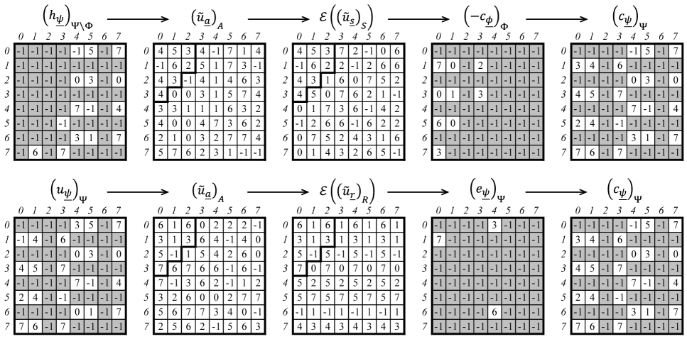
Figure 1: (Top row.) Systematic encoding of the shortened Hermitian code $C^{\perp}(S_{\Phi},\Psi)$ by Algorithm 2. A given information is $\left(h_{\underline{\psi}}\right)_{\Psi\backslash\Phi}$ and the systematic codeword is $\left(c_{\underline{\psi}}\right)_{\Psi}$. (Bottom row.) Its decoding by Algorithm 1. A received word is $\left(u_{\underline{\psi}}\right)_{\Psi}=\left(c_{\underline{\psi}}\right)_{\Psi}+\left(e_{\underline{\psi}}\right)_{\Psi}$.

V Estimation of complexity

We estimate the number of finite-field operations, i.e., additions, subtractions, multiplications, and divisions, in Algorithm 1 for codes (20). For the computation of DFT and IDFT, we employ multidimensional FFT algorithm; it is well-known that its number of finite-field operations is the order of $L\log L$, where $L$ is the data size and $L=q^{N}$ in our case. Summarizing the results, we evaluate the algorithm as follows, where $n$ is code length, $N$ is dimension of $\Omega$, $q$ is finite-field size, and $d$ is the number of elements in Gröbner bases.

Algorithm 1 manipulation order of bound

Step 1 $$\left(\sum_{\underline{\psi}\in\Phi_{1}}\underline{\psi}^{\underline{a}}\right)_{A}$$

Step 2 BMS

Step 3

Step 4 BMS

Step 5

Step 6

Thus the total number of finite-field operations in Algorithm 1 is bounded by the order of $dn^{2}+nq^{N}$. In particular, the number of finite-field operations for calculating error values apart from BMS algorithm has the order of $nq^{N}$. In the proof [5] of $\{\mbox{linear codes}\}=\{\mbox{affine variety codes}\}$, $q^{N}$ is chosen as $q^{N-1}<n\leq q^{N}$, which leads $nq^{N}<qn^{2}$. Thus, if $q<n$, the computational complexity $qn^{2}$ of error-value calculation by Algorithm 1 improves $n^{3}$ by error correcting pairs in [11] and $n^{3}$ by inverse matrices of proper transforms in [12].

References

- [1] H.E. Andersen, O. Geil, “Evaluation codes from order domain theory,” Finite Fields and Their Applications, vol.14, no.1, pp.92–123, Jan. 2008.
- [2] M. Bras-Amorós, M.E. O’Sullivan, “The correction capability of the Berlekamp–Massey–Sakata algorithm with majority voting,” Applicable Algebra in Eng., Commun. Comput., vol.17, no.5, pp.315–335, Oct. 2006.
- [3] D. Cox, J. Little, D. O’Shea, Ideals, Varieties, and Algorithms: An introduction to computational algebraic geometry and commutative algebra, 2nd ed. New York: Springer Publishers, 1997.
- [4] D. Cox, J. Little, D. O’Shea, “The Berlekamp–Massey–Sakata algorithm,” Using Algebraic Geometry, 2nd ed., pp.494–532, Springer, 2005.
- [5] J. Fitzgerald, R.F. Lax, “Decoding affine variety codes using Gröbner bases,” Des. Codes Cryptogr., vol.13, no.2, pp.147–158, Feb. 1998.
- [6] R. Kötter, “A fast parallel implementation of a Berlekamp–Massey algorithm for algebraic-geometric codes,” IEEE Trans. Inf. Theory, vol.44, no.4, pp.1353–1368, Jul. 1998.
- [7] J.B. Little, “The key equation for codes from order domains,” Advances In Coding Theory And Cryptography, pp.1–17, T. Shaska et al. eds., World Scientific Publishing Co. Pte. Ltd., 2007. arXiv:math/0303299v2.
- [8] H. Matsui, S. Mita, “A new encoding and decoding system of Reed–Solomon codes for HDD,” IEEE Trans. on Magnetics, vol.45, no.10, pp.3757–3760, Oct. 2009.
- [9] H. Matsui, “Fast erasure-and-error decoding and systematic encoding of a class of affine variety codes,” 34th Symp. Inf. Theory and Its Applications, pp.405–410, Ousyuku, Iwate, Japan, Nov. 29–Dec. 2, 2011.
- [10] S. Miura, “Linear codes on affine algebraic varieties,” (in Japanese) IEICE Trans. Fundamentals, vol.J81–A, no.10, pp.1386–1397, Oct. 1998.
- [11] R. Pellikaan, “On decoding by error location and dependent sets of error positions,” Discrete Math., vol.106/107, pp.369–381, Sep. 1992.
- [12] K. Saints, C. Heegard, “Algebraic-geometric codes and multidimensional cyclic codes: a unified theory and algorithms for decoding using Gröbner bases,” IEEE Trans. Inf. Theory, vol.41, no.6, pp.1733–1751, Nov. 1995.
- [13] S. Sakata, H.E. Jensen, T. Høholdt, “Generalized Berlekamp–Massey decoding of algebraic geometric codes up to half the Feng–Rao bound,” IEEE Trans. Inf. Theory, vol.41, no.6, Part I, pp.1762–1768, Nov. 1995.
- [14] S. Sakata, D.A. Leonard, H.E. Jensen, T. Høholdt, “Fast erasure-and-error decoding of algebraic geometry codes up to the Feng–Rao bound,” IEEE Trans. Inf. Theory, vol.44, no.4, pp.1558–1564, Jul. 1998.