Temporal percolation of a susceptible adaptive network

Abstract

In the last decades, many authors have used the susceptible-infected-recovered model to study the impact of the disease spreading on the evolution of the infected individuals. However, few authors focused on the temporal unfolding of the susceptible individuals. In this paper, we study the dynamic of the susceptible-infected-recovered model in an adaptive network that mimics the transitory deactivation of permanent social contacts, such as friendship and work-ship ties. Using an edge-based compartmental model and percolation theory, we obtain the evolution equations for the fraction susceptible individuals in the susceptible biggest component. In particular, we focus on how the individual’s behavior impacts on the dilution of the susceptible network. We show that, as a consequence, the spreading of the disease slows down, protecting the biggest susceptible cluster by increasing the critical time at which the giant susceptible component is destroyed. Our theoretical results are fully supported by extensive simulations.

1 Introduction

Dynamic topologies in complex network models have recently become a subject of intensive investigations [1, 2]. While in the past, many dynamical processes were mainly developed numerically and analytically on static networks, most of the real networks alter their topologies over time. As a consequence, recently many researchers are modeling these processes on top of dynamic networks. The topology of the networks can change by evolution or by adaptive dynamic [1, 2]. Those networks in which the structure changes regardless of the processes taking place on top of them are called evolutive networks. On the other hand, networks that alter their topology to mitigate or promote these processes are called adaptive networks [1, 3, 4]. In adaptive networks, there is a co-evolution between the dynamic process and the topology. The study of adaptive networks has generated a great interest in many disciplines since there is evidence of many real systems with an adaptive topology [1]. For example, from the analysis of the gene regulatory networks, it was shown that interactions between genes can change in response to diverse stimuli, leading to changes in the network’s topology [5, 1]. On the other hand, the recent pandemics of SARS [6] and H1N1 [7], have promoted the modeling of adaptive strategies on the contact network to slow down the spread of the epidemics [8, 9, 10, 11, 12, 13]. The study of these mitigation strategies could provide important information to adopt health policies, allowing to characterize the effect of the strategy on the structure of the society and to quantify its effectiveness against the spread of an epidemic.

The most used model that represents these recent diseases is the susceptible-infected-recovered (SIR) model [14, 15], in which the individuals can be in one of three states, susceptible, infected or recovered. In this model, the disease propagates on top of the contact network until it reaches the steady state, i.e., when there are no more infected individuals. In static networks, the steady state of the SIR model was widely studied using percolation tools through a generating function formalism [16, 17, 18, 19]. It is known that the final size of the disease (fraction of recovered individuals) is governed by a control parameter which is the effective probability of infection or transmissibility $T$ of the disease. At a critical threshold $T=T_{c}$, the disease overcomes a second order phase transition with an epidemic phase for $T>T_{c}$, while for $T<T_{c}$ the disease consists only of outbreaks that reach a small fraction of the population.

In the last decade, there has been considerable progress to described theoretically the dynamics of the disease spreading of this model in static networks [20, 21, 22, 23, 24]. However these researches have only focused on the description of the temporal evolution of compartmental quantities, such us the fraction of the infected and susceptible individuals. Recently, Valdez et al. [25] using an edge-based compartmental model (EBCM) [20, 21, 22] and a generating function formalism, proposed a set of equations which describe the evolution of the size of the giant component of the susceptible individuals (GSC) in static networks. They found that a time-dependent quantity $\Phi_{S}(t)$, namely, the probability that a given neighbor of a root node is susceptible at time $t$ (more details are given below), is the control parameter of a temporal node void percolation process involving the network composed by susceptible individuals. They showed that the GSC overcomes a second order phase transition at a critical time $t_{c}$ above which it is destroyed.

In contrast to the SIR model in static networks, the study of this model on adaptive topologies has being explored by few authors. Wang et al. [12] proposed an intervention strategy in which susceptible individuals, induced by fear, break the links with their neighbors, with a probability related to the number of infected neighbors, regardless of the state of the neighbors. They show that this strategy decreases the number of infected individuals and delays the progression of the disease compared to the case of non-intervention. Lagorio et al. [26] studied a rewiring strategy in which susceptible individuals redirect their links with infected neighbors towards other susceptible individuals with probability $w$. They showed that there is a phase transition at a critical rewiring threshold $w_{c}$ separating an epidemic from a non-epidemic phase, which can be related to static link percolation. In a recent paper [27], it was proposed an adaptive SIR model driven by intermittent connections where the susceptible individuals, using local information, break the links with their infected neighbors with probability $\sigma$ for an interval $t_{b}$ after which they reestablish the connections with their previous contacts. This model, called intermittent social distancing (ISD) strategy focus to model the behavior of individuals who preserve their closer contacts during the disease spreading. Using the framework of percolation theory, they derived the transmissibility $T_{\sigma}$ and found that there exists a critical probability $\sigma_{c}$ depending on $t_{b}$, above which the epidemic spread is stopped. They also showed that the ISD strategy, produces a “susceptible herd behavior” below a transmissibility $T^{*}$ [27, 28] that protects a large cluster of susceptible individuals from being infected. This focus on the susceptible network provides a description of the functional network, since the GSC is the one that supports the economy of a society.

Until now, these researches have focused on the effect of the strategies on quantities in the steady state and very little has made to describe the dynamics. Moreover, so far less explored, is the study of the effect of these strategies on the GSC.

In this paper, using the EBCM approach and percolation theory, we study the temporal evolution of the fraction of the susceptible individuals on adaptive networks following the ISD strategy. We find that this strategy protects a giant susceptible cluster by increasing the time $t_{c}$ at which the functional network is destroyed. In a more realistic scenario where the implementation of the strategy is delayed, we obtain that it also increases $t_{c}$, and find that the dilution of the GSC can also be described theoretically by percolation tools. The paper is organized as following: in Sec. 2, we explain the node void percolation that describes the dilution of the susceptible network. In Sec. 3 we derive the dynamic equations of the ISD strategy and in Sec. 4 we present the theoretical and the simulation results of the ISD strategy implemented from the beginning of the disease spreading. In Sec. 5 we derive the evolution equations when the implementation of the strategy is delayed. Finally, in Sec. 6 we present our conclusions and outlooks.

2 Framework of Node Void Percolation

In the discrete version of the SIR model, an infected individual infects a susceptible neighbor with probability $\beta$ and he recovers after $t_{r}$ time units since he was infected, where $t_{r}$ is called the recovery time. It is known that in this model the control parameter is the transmissibility $T=1-(1-\beta)^{t_{r}}$ that governs the final fraction of infected individuals. This model can be mapped into link percolation since when the disease traverses a link with a transmissibility $T$, this process is equivalent to occupy that link with the same probability $T$.

On the other hand, the network composed by susceptible individuals is diluted during the epidemic spreading, since when the disease traverses a link, the susceptible individual is removed from the susceptible network. However, this process is different than an ordinary node percolation because the susceptible nodes are not chosen randomly. Instead, they are reached by the disease following a link, and therefore, nodes with higher connectivity are reached with higher probability than nodes with lower connectivity. This kind of dilution, that we called node void percolation [25] leads, in the steady state, to a second order phase transition in which the order parameter is the fraction of nodes $S_{1}$ in the GSC, and the control parameter is $\Phi_{S}(\infty)$, i.e., the probability that following a random chosen link, a susceptible node is reached. Moreover, since the susceptible network loses the nodes with the highest connectivities, the phase transition at $\Phi_{S}(\infty)=\Phi_{Sc}$, has mean field exponents, as in an intentional attack process independently of the network’s topology [29, 25].

When $T$ increases, $S_{1}$ decreases and therefore $\Phi_{S}(\infty)$ and $T$ are interrelated. In particular, there is an effective transmissibility $T^{*}$ that set the critical value of $\Phi_{Sc}$ at which $S_{1}\to 0$, and its value can be obtained using a generating function formalism [27, 28]. Denoting the degree distribution as $P(k)$, $T^{*}$ fulfills the equation

$$\Phi_{Sc}=G_{1}[1-T^{*}(1-\Phi_{Sc})],$$ (1)

where $T^{*}$ is the solution of Eq. (1), $\Phi_{Sc}=G_{1}\left[(G_{1}^{{}^{\prime}})^{-1}(1)\right]$ and $G_{1}(x)=\sum_{k}kP(k)/\langle k\rangle x^{k-1}$ is the generating function for the excess degree distribution, that is, the degree distribution of the remaining outgoing links in a branching process [30, 31].

3 Dynamic framework of the ISD strategy

In the ISD model, initially all the nodes are susceptible except for one node randomly infected, that represents the patient zero from which the disease spreads. In this paper, we call active links to the links between infected and susceptible individuals. An infected individual transmits the disease to a susceptible neighbor with probability $\beta$ and, if he fails, the susceptible individual breaks his link with the infected one with probability $\sigma$ for $t_{b}$ time units. After a period $t_{b}$ both individuals are reconnected and the process is repeated until the infected individual recovers at a fixed time $t_{r}>t_{b}$ since he was infected. If an active link is broken for more than $t_{b}=t_{r}-1$ time units, it is restored as a non-active link since the infected individual is recovered. In this model, the disease spreads with an effective transmissibility $T(\beta,\sigma,t_{r},t_{b})\equiv T_{\sigma}$ [27] given by,

$$T_{\sigma}=\sum_{m=1}^{t_{r}}\beta(1-\beta)^{m-1}(1-\sigma)^{m-1}+\beta\sum_{m=t_{b}+2}^{t_{r}}\phi(m,t_{b},\sigma,\beta).$$ (2)

In the first term of Eq. (2), $\beta(1-\beta)^{m-1}(1-\sigma)^{m-1}$ is the probability that an active link is lost due to the infection of the susceptible individual at time $m$ given that the active link has never been broken in the $m-1$ steps since it appears. In the second term of Eq. (2), $\beta\;\phi(m,t_{b},\sigma,\beta)$ denotes the probability that an active link is lost due to the infection of the susceptible individual at time $m$ given that the link was broken at least once in the first $m-1$ time units. The probability $\phi(m,t_{b},\sigma,\beta)$, which is only valid for $m\geq t_{b}+2$ is given by [27]

$$\phi(m,t_{b},\sigma,\beta)\equiv\phi_{m}=\sum_{u=1}^{\left[\frac{m-1}{t_{b}+1}\right]}\binom{m-u\;t_{b}-1}{u}\sigma^{u}(1-\sigma)^{m-1-u(t_{b}+1)}(1-\beta)^{m-1-u\;t_{b}},$$ (3)

where $\left[\cdots\right]$ denotes the integer part function. Thus, the ISD strategy [27] reduces the initial transmissibility $T$ towards an effective transmissibility $T_{\sigma}$, mitigating the spread of the disease.

Eq. (2) can be rewritten as

$$T_{\sigma}=\beta\sum_{m=1}^{t_{r}}\Omega_{m},$$ (4)

with

$$\Omega_{m}\equiv(1-\beta)^{m-1}(1-\sigma)^{m-1}+\phi_{m},$$ (5)

where $\Omega_{m}$ is the probability that an active link has neither ever transmitted the disease nor been broken during the first $m-1$ time units, plus the probability that the active link was broken at least once in the first $m-1$ time units but at time $m$ it is present. Here, $\phi_{m}=0$ for $m<t_{b}+2$ and is given by Eq. (3) for $t_{b}+2\leq m\leq t_{r}$.

In order to study the evolution of the number of infected and susceptible individuals in the ISD model, we use the edge-based compartmental approach [20, 21, 22] based on a generating function formalism. Denoting the fraction of susceptible, infected and recovered individuals at time $t$ by $S(t)$, $I(t)$ and $R(t)$, respectively, the EBCM approach lies on describing the evolution of the probability that a randomly chosen node is susceptible. In order to compute $S(t)$, a link is randomly chosen and then a direction is given, in which the node in the target of the arrow is called the root, and the base is its neighbor. Then the fraction of susceptible individuals is given by $S(t)=\sum_{k}P(k)\theta_{t}^{k}=G_{0}(\theta_{t})$, where $G_{0}(x)$ is the generating function of the degree distribution and $\theta(t)\equiv\theta_{t}$ is the probability that the base does not transmit the disease to the root. In this approach, infection from the root to the base is disallowed, in order to treat the state of the root’s neighbors as independent [21, 22]. In order to find $\theta_{t}$ we have to compute the probabilities $\Phi_{S}(t)$, $\Phi_{R}(t)$ and $\Phi_{I}(t)$ that the base is susceptible, recovered or infected but has not yet transmitted the disease to the root. These probabilities satisfy the relation

$$\Phi_{S}(t)+\Phi_{I}(t)+\Phi_{R}(t)=\theta_{t}.$$ (6)

As $\Phi_{S}(t)$ depends on the second neighbors of the root, we have to disallow infection from the first neighbor (base of the root) to the second neighbors, thus

$$\Phi_{S}(t)=G_{1}(\theta_{t}).$$ (7)

Then, using the EBCM approach adapted to discrete times, the evolution of $\Phi_{S}(t)$ and $\Phi_{I}(t)$ in the ISD model is given by deterministic equations, that are only valid above the critical transmissibility $T_{c}$ where there is a macroscopic fraction of infected nodes,

$$\Delta{\theta_{t}} = -\beta\Phi_{I}(t),$$ (8)

$$\Delta{\Phi}_{S}(t) = G_{1}(\theta_{t+1})-G_{1}(\theta_{t}),$$ (9)

where $\Delta$ is the discrete change of the variables between times $t$ and $t+1$. Eq. (8) represents the decrease of $\theta_{t}$ when the disease traverses an active link. Eq. (9) describes the decrease of $\Phi_{S}(t)$ (see Eq. (7)). It is important to note that $\Delta\Phi_{S}(t)$ is non-positive, and $-\Delta\Phi_{S}(t)$ represents the new active links.

The evolution equation of $\Phi_{I}(t)$ is given by,

$$\Delta{\Phi}_{I}(t) = -\beta\Phi_{I}(t)-\Delta{\Phi}_{S}+(1-\beta)(1-\sigma)\;\Omega_{t_{r}}\Delta{\Phi}_{S}(t-t_{r})+\Psi(t),$$ (10)

where

$$\Psi(t) \equiv -\sigma(1-\beta)\Phi_{I}(t)+\sigma(1-\beta)\Phi_{I}(t-t_{b})$$ (11)

$$+\sum_{i=0}^{t_{b}}\sigma(1-\beta)\Omega_{t_{r}-t_{b}+i}\Delta{\Phi}_{S}(t-i-t_{r}),$$

with,

$$\Omega_{t_{r}-t_{b}+i}=(1-\beta)^{t_{r}-t_{b}+i-1}(1-\sigma)^{t_{r}-t_{b}+i-1}+\phi_{t_{r}-t_{b}+i},$$ (12)

already defined by Eq. (5).

In Eq. (10) the first term represents the decrease of $\Phi_{I}(t)$ when the infected base node transmits the disease to the root; the second term corresponds to an increasing of $\Phi_{I}(t)$ due to the new infections. The third term corresponds to the recovery of the infected nodes in active links, which is proportional to: a) the active links that appeared $t_{r}$ time units ago i.e., $\Delta{\Phi}_{S}(t-t_{r})$ and b) to the probability that these active links are present $t_{r}-1$ time units after they appeared and in the last time unit they do not transmit the disease neither being broken, i.e., $(1-\beta)(1-\sigma)\Omega_{t_{r}}$. Note that $\Omega_{t_{r}}\Delta{\Phi}_{S}(t-t_{r})$ is related with the active links that appeared $t_{r}$ time units ago, and remain active in their last time unit before the nodes recover and the active links disappear. The last term corresponds to breaking and reconnection of active links [see Eq. (11)].

The first term of Eq. (11), which we call “breaking term”, represents the decrease of $\Phi_{I}(t)$ due to breaking active links during a period $t_{b}$, which is proportional to $\sigma(1-\beta)$. The remaining terms, which we call “reconnection terms”, represent the increase of $\Phi_{I}(t)$ due to reconnecting active links. While the reconnection term could be thought as minus the “breaking term” delayed by $t_{b}$ time units [i.e., $\sigma(1-\beta)\Phi(t-t_{b})$], that term needs to be corrected due to the recovery of some infected individuals that reduce the number of active links that could be restored at time $t+1$. In Table 1 we show a schematic with an example of the correction term. Then $\Psi(t)$ [see Eq. (11)] represents the net flow between the decrease of the probability $\Phi_{I}(t)$ due to breaking active links, and the increase of $\Phi_{I}(t)$ due to restoring active links that have being disconnected $t_{b}$ units time ago.

Table 1: Schematic cases of the “reconnection terms” of Eq. (11) for $t_{r}=10$ and $t_{b}=4$. The first column represents a typical configuration of different cases of the “reconnection term”. The second column is the probability that an active link cannot be restored at time $t$. In the first column, each cell corresponds to a unit time. The white cells represent the time unit at which an active link between the susceptible and the infected node exists, the gray ones represent to the disconnection period and the crosses correspond to the case where the infected is recovered. The moment at which an active link appears is represented by (I), and the moment when this pair, at time $t-t_{b}$, breaks for the next $t_{b}$ time units is represented by (II). When some active links break at time $t-t_{b}$ at the beginning of time $t$ they have to be restored, which is the case of 1). However, other active links which break at time $t-t_{b}$ cannot be restored as active links because the infected node recovers. This is shown in the cases 2a) and 2b) where the infected node has recovered at $i=2$ time units before $t$ (where $i$ is the sub-index of Eq. (12)). The case 2a), corresponds to an active link which appears at time $t-t_{r}-i=t-12$ and breaks by the first time $8$ times unit later. The probability for this case is $\sigma(1-\beta)^{8}(1-\sigma)^{7}$. Similarly, the case 2b) corresponds to an active link which appears at time $t-t_{r}-i=t-12$ and breaks, but not by the first time, $8$ time units later. The probability of this case is $\sigma(1-\beta)\phi_{8}$.

Example	Probability that the active link cannot be restored at time $t$
	0
	$\sigma(1-\beta)^{8}(1-\sigma)^{7}$
	$\sigma(1-\beta)\phi_{8}$

Note that in Eq. (11), $(1-\beta)\sigma$ is the probability that an active link breaks. By contrast, $\Phi_{I}(t)$ corresponds to the state of the base node and no information is provided about the state of the root node. Therefore, Eqs. (10) and (11) correspond to a process wherein the infected nodes break their links with infected and recovered individuals too. However, the breaking of these links has no effect on the evolution of $I(t)$ and $S(t)$ because those links are not able to transmit the disease. Therefore, Eqs. (10) and (11) are also valid for our ISD strategy, where only the susceptible individuals break their links with the infected ones.

The evolution of the fraction of infected individuals is given by [25]

$$\Delta{I}(t) = -\Delta S(t)+\Delta S(t-t_{r}),$$ (13)

where $-\Delta S(t)=-(G_{0}(\theta_{t+1})-G_{0}(\theta_{t}))$, as explained above, represents the fraction of new infected individuals. The second term represents the decrease of $I(t)$ due to the recovery of infected individuals that have been infected $t_{r}$ time units ago. Note that $I(t)$ contains the new infected individuals at time $t$, and also the infected in a previous time.

The evolution of the fraction of susceptible individuals in the susceptible giant component $S_{1}(t)$ is obtained [25] by solving the equations

$$S_{1}(t) = G_{0}(\theta_{t})-G_{0}(\omega_{t}),$$ (14)

$$\omega_{t} = \theta_{t}-G_{1}(\theta_{t})+G_{1}(\omega_{t}),$$ (15)

where $\omega_{t}$ is the probability that a base individual, which is not connected to the giant susceptible cluster, has not yet transmitted the disease to the root at time $t$; $G_{0}(\theta_{t})=S(t)$ is the total fraction of susceptible individuals and $G_{0}(\omega_{t})$ is the fraction of individuals belonging to finite susceptible clusters. In this paper, we only present our theoretical and numerical results for the susceptible nodes, because we are interested here only on the functional network. However, we checked that Eq. (13) is in fully agreement with the simulations for the ISD strategy.

4 Theoretical and simulation results

We apply the ISD strategy on Erdös Rényi networks (ER) with degree distribution $P(k)=\langle k\rangle^{k}\exp(-\langle k\rangle)/k!$, in which $k$ is the connectivity and $\langle k\rangle$ is the average degree of the network, and Scale-Free networks (SF) with degree distribution $P(k)\sim k^{-\lambda}$ where $k_{min}\leq k\leq k_{max}$ and $\lambda$ is a measure of the heterogeneity of the degree distribution.

In order to obtain theoretically $S_{1}(t)$, we iterate Eqs. (8)-(14) with initial condition $\theta_{0}=1-1/N$, $\Phi_{I}(0)=1/N$ where $N$ is the number of nodes in the network. Since at the beginning of the spreading the fraction of infected individuals is very small, the time $t$ is shifted to $t=0$ when $1$% of the individual are infected [20] because this stochastic regime is not taken into account in our deterministic equations.

For the numerical simulations we construct the networks using the configurational model  [32], and for the disease propagation we use the algorithm explained in Sec. 3. For SF networks, we choose $k_{min}=2$ in order to ensure that the network is fully connected [33]. In the simulations, the disease has a transmissibility $T$ without strategy, but it will spread with transmissibility $T_{\sigma}$ [see Eq. (2)] due to the ISD strategy that is applied since the patient zero appears.

In Fig. 1 we plot the time evolution of the size $S_{1}(t)$ of the GSC, for ER and SF networks with the same average degree, obtained from the theory and the simulations, where we call “size” to the fraction of nodes belonging to a cluster or component. Remarkably, from the plots we can see the total agreement between the theory and the simulations which shows that a complete description of the time evolution of the size of the GSC can be given in this adaptive strategy using theoretical tools [34]. On the other hand, we also plot the size of the second biggest susceptible cluster $S_{2}(t)$, in order to show the time at which the phase transition develops on the GSC. This critical time is an important quantity since it suggests that an intensification of the strategy is needed in order to prevent or delay the destruction of the functional GSC.

\begin{overpic}[scale={0.24}]{Fig03.eps} \put(70.0,50.0){{\bf{(a)}}} \end{overpic}

\begin{overpic}[scale={0.24}]{Fig04.eps} \put(70.0,50.0){\bf{(b)}} \end{overpic}

Figure 1: Time evolution of the size of the susceptible giant cluster $S_{1}(t)$ (black) and the second susceptible component $S_{2}(t)$ (red), for $N=10^{5}$, $t_{r}=20$, $\beta=0.05$ ($T=0.64$) without intervention ($\bigcirc$) and with the ISD strategy for $\sigma=0.50$ and $t_{b}=1$ ($\square$, $T_{\sigma}=0.50$) and $t_{b}=2$ ($\lozenge$, $T_{\sigma}=0.41$) with $\langle k\rangle=4$ in an ER network ($T^{*}=0.46$ and $T_{c}=0.25$) (a) and a SF with $\lambda=2.63$, $k_{min}=2$ and $k_{max}=500$ ($T^{*}=0.40$ and $T_{c}=0.05$) (b). The symbols correspond to the simulations and the solid lines are obtained from Eq. (14). The dashed lines of the $S_{2}(t)$ curves are used as guides for the eyes. (Color online).

As shown in the figure, the strategy increases the critical time $t_{c}$ compared to the case without mitigation strategy ($\sigma=0$), due to the fact that as $t_{b}$ and $\sigma$ increases, the effective transmissibility $T_{\sigma}$ decreases together with the number of links traversed by the disease, protecting the GSC during a greater period of time. In order to quantify $t_{c}$, we measure the position of the peak of $S_{2}(t)$ (see Fig. 1), which corresponds to the average time at which the GSC is destroyed. In Fig. 2 we plot in the plane $t_{b}-\sigma$, $\Delta t_{c}=t_{c}(\sigma)-t_{c}(\sigma=0)$ for different values of $\sigma$ and $t_{b}$, obtained from the simulations.

\begin{overpic}[scale={0.24}]{Fig05.eps} \put(80.0,35.0){{\bf{(a)}}} \end{overpic}

\begin{overpic}[scale={0.24}]{Fig06.eps} \put(70.0,40.0){\bf{(b)}} \end{overpic}

Figure 2: Phase diagram $t_{b}-\sigma$ displaying the increasing $\Delta t_{c}$ of the critical time from the case without intervention, for different values of $\sigma$ and $t_{b}$, $N=10^{5}$, $t_{r}=20$, $\beta=0.05$ with $\langle k\rangle=4$ in an ER network ($T^{*}=0.46$) (a) and a SF with $\lambda=2.63$, $k_{min}=2$ and $k_{max}=500$ ($T^{*}=0.40$) (b). The lowest increasing is in black color, and the highest in white color. The dashed lines correspond to the case $T_{\sigma}=T^{*}$ (Color online).

From Fig. 2 we observe that the finite values of $\Delta t_{c}$ only correspond to $T_{\sigma}>T^{*}$ [see Eq. (1)]. We can also see that the value of $\Delta t_{c}$ increases when $T_{\sigma}\to T^{*}$ from above, because below $T^{*}$ the GSC is never destroyed. In SF networks, this increasing is less sensitive to the ISD strategy than in ER networks, which is expected since in the former, the infected nodes with high connectivities tend to enhance the disease spreading, decreasing $S_{1}(t)$ at earlier times. However, there is a large range of values of $t_{b}$ and $\sigma$ that allow to protect the giant susceptible cluster for diseases with not too high values of $\beta$ [35, 27]. The ability to decrease the transmissibility of the disease spreading is an advantage of the ISD strategy for the susceptible network since it gives to the public health authorities more time to implement other policies, such as vaccination and to alert the health services, before the functional network composed by healthy people disappears.

5 Delayed implementation of the ISD strategy

While most of the adaptive strategies are applied at the beginning of the disease spreading, in real situations, a mitigation strategy is rarely implemented when the first infected appears [36, 37] because at this stage the health authorities ignore the severity of the disease or they are cautious to declared the alert of an epidemic since any strategy could affect the functional susceptible network. In this section, we study the performance of the strategy when it is implemented at a different time after the beginning of the disease spreading.

In order to obtain the evolution equations of the delayed ISD strategy, we consider that this strategy is implemented when a fraction $x$ of the population is not susceptible.

If we denote $J(t)=I(t)+R(t)$, where $J(t)$ is the fraction of the population that was reached by the spread (incidence curve), when $J(t)<x$, the evolution of the disease spreading on top of a static network is governed by the Eqs. (8), (9), (13)-(15), except for $\Phi_{I}(t)$, that is given by [25],

$$\Delta{\Phi}_{I}(t) = -\beta\Phi_{I}(t)-\Delta{\Phi}_{S}(t)+(1-T)\Delta{\Phi}_{S}(t-t_{r}).$$ (16)

When $J(t)\geq x$ at $t=\tau$, the ISD strategy is implemented and the evolution of the spreading follows Eqs. (8)-(10), (13)-(15). However, note that when $J(\tau)=x$, there is a change in the transmissibility, since just after the disease reaches $x$ percent of the population, there are still some active links that appeared before $t=\tau$, which we call “old links”. As a consequence, the effective probability that these links would be traversed at early stages is not $T$ neither $T_{\sigma}$. In order to incorporate this issue in the evolution equations, first we have to compute $\Phi_{I,z}\equiv(1-\beta)^{t_{r}-z}\Delta\Phi_{S}(\tau-t_{r}+z)$, i.e., the amount of old active links which appeared $t_{r}-z$ times units before $t=\tau$. This is equivalent to have a smaller recovery time $z$ (with $1\leq z\leq t_{r}-1$) instead of $t_{r}$, in the evolution equations of the ISD strategy . As a consequence, the probability that these old links have not yet transmitted the disease at time $t=\tau+j$ with $j\leq z$ is $\Omega_{j}$ (see Eq. (5)). Here, we consider $\Omega_{j}=0$ for $j<1$ and $j>t_{r}-1$ for the case of old links. Then, the equation of $\Phi_{I}(t)$ for the delayed ISD strategy needs to take into account the old active links, thus

$$\Delta{\Phi}_{I}(t) = -\beta\Phi_{I}(t)-\Delta{\Phi}_{S}+(1-\beta)(1-\sigma)\Omega_{t_{r}}\Delta{\Phi}_{S}(t-t_{r})\Theta_{1}+$$ (17)

$$+(1-\beta)(1-\sigma)\Omega_{t-\tau+1}\Phi_{I,t-\tau+1}(1-\Theta_{1})+\Psi^{*}(t),$$

with

$$\Psi^{*}(t) \equiv -\sigma(1-\beta)\Phi_{I}(t)+\sigma(1-\beta)\Phi_{I}(t-t_{b})\Theta_{0}$$ (18)

$$+\left(\sum_{i=0}^{t_{b}}\sigma(1-\beta)\Omega_{t_{r}-t_{b}+i}\Delta{\Phi}_{S}(t-i-t_{r})\right)\Theta_{1}$$

$$+\left(\sum_{z=t-\tau-t_{b}}^{t-\tau}\sigma(1-\beta)\Omega_{t-\tau-t_{b}}\Phi_{I,z}\right)(1-\Theta_{2}),$$

where $\Theta_{0}$, $\Theta_{1}$ and $\Theta_{2}$ are the Heaviside functions given by

$$\Theta_{0}=\left\{\begin{array}[]{cl}0&\mbox{if }\;\;\;t<\tau+t_{b}-1\\ 1&\mbox{otherwise }\end{array}\right.\\ ,\Theta_{1}=\left\{\begin{array}[]{cl}0&\mbox{if }\;\;\;t<\tau+t_{r}-1\\ 1&\mbox{otherwise }\end{array}\right.\\ ,$$

$$\Theta_{2}=\left\{\begin{array}[]{cl}0&\mbox{if }\;\;\;t<\tau+t_{r}+t_{b}-1\\ 1&\mbox{otherwise }\end{array}\right.$$

The first two terms of Eq. (17) are the same as those in Eq. (10). The third term corresponds to the recovery of the active links which appeared at time $t\geq\tau-1$. This term is different from zero only after $t_{r}-1$ time units since $\tau$, and has the same form as the third term of Eq. (10). The fourth term describes the recovery of the infected individuals of old active links. Note that this term, has the same form as the previous one, in which $\Phi_{I,t-\tau+1}$ plays the role of $\Delta{\Phi}_{S}(t-t_{r})$. Finally the fifth term corresponds to the breaking-reconnection term that is similar to Eq. (11).

In Eq. (18), the first two terms are similar as those in Eq. (11). The third term corresponds to the correction on the reconnection term due to the recovery of infected individuals of the active links that appear after $t=\tau$. On the other hand, the last term corresponds to the correction due to the recovery of the infected individuals of the old links. In Fig. 3 we show a schematic of this term.

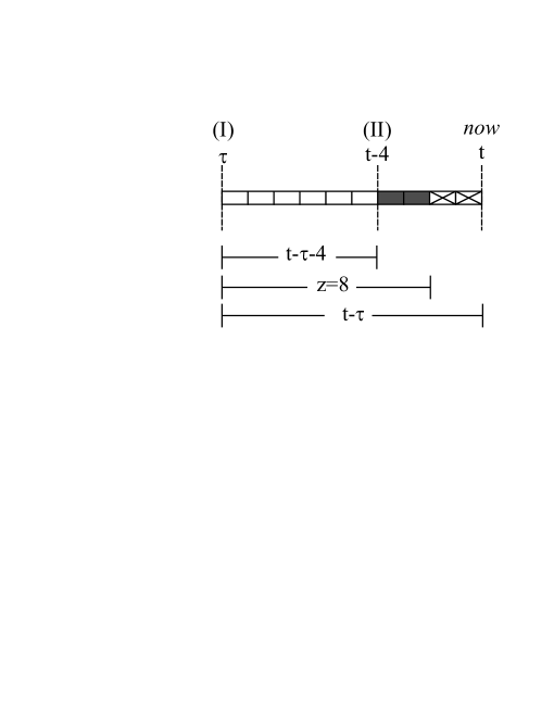
Figure 3: Schematic of the correction of the restoring term of Eq. (18) at time $t$, for an old active link with $z=8$ and $t_{b}=4$ that breaks two units time before the infected node recovers. Each cell corresponds to a time unit. The white cells represent the time unit at which an active link between the susceptible and the infected node exists, the gray ones denote the disconnection period and the crosses correspond to the case where the infected is recovered. The moment $\tau$ at which the ISD strategy is implemented, is represented by (I), and the moment when this active link, at time $t-t_{b}$, breaks for the next $t_{b}$ time units is denoted by (II). The fraction of active links represented in the plot is proportional to $(1-\beta)\sigma\Omega_{t-\tau-4}$.

In Fig. 4 we plot $S_{1}(t)$ as a function of $t$ for ER and SF networks, when the ISD strategy is applied after the disease reaches a fraction $x$ of the population.

\begin{overpic}[scale={0.26}]{Fig08.eps} \put(80.0,30.0){{\bf{(a)}}} \end{overpic}

\begin{overpic}[scale={0.26}]{Fig09.eps} \put(80.0,30.0){\bf{(b)}} \end{overpic}

Figure 4: $S_{1}(t)$ for a disease with $t_{r}=20$, $\beta=0.10$ ($T=0.88$) and $N=10^{5}$ when the ISD strategy (with $\sigma=0.50$ and $t_{b}=10$, i.e., $T_{\sigma}=0.33$) is applied at different moments: never (black, $\bigcirc$), after the disease reaches 25% ($x=0.25$) of the population (red, $\triangle$), and from the beginning (blue, $\square$) for an ER network with $\langle k\rangle=4$ (a) and a SF network with $\lambda=2.63$, $k_{min}=2$ and $\langle k\rangle=4$ (b). The symbols correspond to the simulations with 100 network realizations, and the solid lines correspond to the theoretical solutions. In ER network, for the case with strategy applied from the beginning $S_{1}(t\to\infty)=0.47$. (Color online).

As shown in the figure, the strategy can protect a GSC, even when it is applied after a large fraction of the population is infected. Note that the delayed strategy does not change the behavior of the order parameter $S_{1}(t)$ with $\Phi_{S}(t)$, thus, the critical value of $\Phi_{Sc}$ at which the giant susceptible cluster is destroyed remains invariant (see Appendix). On the other hand, the strategy protects a smaller fraction of individuals in the functional network in SF than in an ER networks, because in the former the dilution process of the susceptible network is more efficient due to the nodes with high connectivities (see Sec. 2). However, a delayed intermittent connection strategy can still protecting the GSC by increasing $t_{c}$, and thus mitigating the demand of health services and protecting the functional network for an extended period of time.

6 Conclusions

In this paper, we study how individuals based on local information, contribute to halt the epidemic spreading implementing an ISD strategy during a disease spreading. This model where the healthy individuals avoid contact with the infected ones intermittently, allows to mimic a behavioral response of individuals who try to protect themselves from the disease but also try to preserve their closer contacts, such as friendship and working partners.

Using an edge-based compartmental model combined with percolation theory, we show that this strategy increases the critical time at which the susceptible giant component is destroyed, giving more time to the health authorities to implement other policies against the disease spreading. We also study a more realistic scheme in which the strategy is delayed, and found that it also protects the functional network. We show that the dilution of the GSC for the delayed strategy can also be described by percolation theory. Our theoretical framework are fully supported by extensive simulations.

We believe that to focus on the susceptible network and its topological properties, instead that on the infected network, provides a novel description that could be useful for the health services to develop new strategies to protect the society and the economy of a region. Finally, this complementary view of an epidemic spreading could give a new criterion to evaluate the effectiveness of any strategy.

Appendix A Node Void Percolation in a delayed ISD strategy

A feature of the delayed strategy is that the disease spreads with two different values of the transmissibility ($T$ before applying the strategy and $T_{\sigma}$ during the strategy), and thus the final epidemic size cannot be related with a unique value of the control parameter $T$.

In order to study the effect of the delayed strategy on the dilution of the susceptible network, we analyze the relation between $S_{1}(t)$ and $\Phi_{S}(t)$ during the disease spreading. In Fig. 5 we plot $S_{1}(t)$ as a function of $\Phi_{S}(t)$, obtained from the theory (see Eqs. (8)-(15)) and the simulations, when the ISD strategy is applied after the disease reaches a fraction $x$ of the population, for ER and SF networks.

\begin{overpic}[scale={0.19}]{Fig10.eps} \put(80.0,20.0){{\bf{(a)}}} \end{overpic}

\begin{overpic}[scale={0.19}]{Fig11.eps} \put(80.0,20.0){\bf{(b)}} \end{overpic}

\begin{overpic}[scale={0.19}]{Fig12.eps} \put(80.0,20.0){{\bf{(c)}}} \end{overpic}

\begin{overpic}[scale={0.19}]{Fig13.eps} \put(80.0,20.0){\bf{(d)}} \end{overpic}

\begin{overpic}[scale={0.19}]{Fig14.eps} \put(80.0,20.0){{\bf{(e)}}} \end{overpic}

\begin{overpic}[scale={0.19}]{Fig15.eps} \put(80.0,20.0){\bf{(f)}} \end{overpic}

Figure 5: $S_{1}(t)$ as a function of $\Phi_{S}(t)$ for a disease with $t_{r}=20$, $\beta=0.10$ ($T=0.88$) and $N=10^{5}$ (with $\sigma=0.50$ and $t_{b}=10$, i.e., $T_{\sigma}=0.33$) when the ISD strategy is applied at different moments: never (black, $\bigcirc$), after the disease reaches 25% ($x=0.25$) of the population (red, $\triangle$), and from the beginning (blue, $\square$) for an ER network with $\langle k\rangle=4$ [Figs. a), b), c)] and a SF network with $\lambda=2.63$, $k_{min}=2$ and $\langle k\rangle=4$ [Figs. d), e), f)]. The symbols correspond to the simulations with 100 network realizations and the solid black lines are the solution of Eqs. (8)-(15) for the case without strategy. The time $t$ is implicit, and increases when $\Phi_{S}(t)$ decreases. The arrows with label $1$ represent the moment at which the strategy is applied, and the ones with label $2$ correspond to the steady state for the ISD strategy. (Color online).

Even thought there is not a fixed transmissibility, as shown in Fig. 5, the delayed strategy does not change the behavior of the order parameter $S_{1}(t)$ with $\Phi_{S}(t)$ found in the case without intervention [25]. This result is expected since although the speed at which the susceptible giant cluster is diluted changes, the size of the GSC at time $t$ depends on the amount of susceptible nodes removed by node void percolation, and not directly on the transmissibility. As a consequence, the relation between $S_{1}(t)$ and $\Phi_{S}(t)$ holds even for a varying transmissibility. Then, the critical value of $\Phi_{Sc}$ at which the GSC is destroyed remains invariant. This implies that in a realistic scenario in which the transmissibility is varying, if $\Phi_{S}(t)$ is approaching to $\Phi_{Sc}$, the GSC is near to being destroyed. Thus the value of the distance to the criticallity of the susceptible network $\Phi_{S}(t)-\Phi_{Sc}$, could be a crucial information for the authorities to decide if more aggressive health policies are needed to halt the epidemic spreading and to protect the functional network.

References

- [1] T. Gross, H. Sayama, Adaptive Networks: Theory, Models and Applications, Springer, 2009.
- [2] T. Gross, B. Blasius, Journal of The Royal Society Interface 5 (20) (2008) 259–271.
- [3] I. B. Schwartz, L. B. Shaw, Rewiring for adaptation, Physics 3 (2010) 17.
- [4] F. Vazquez, V. M. Eguíluz, M. S. Miguel, Phys. Rev. Lett. 100 (2008) 108702.
- [5] N. M. Luscombe, M. Madan Babu, H. Yu, M. Snyder, S. A. Teichmann, M. Gerstein, Nature 431 (2004) 308–312.
- [6] V. Colizza, A. Barrat, M. Barthelemy, A. Vespignani, BMC Medicine 5 (2007) 34.
- [7] P. Bajardi, C. Poletto, J. J. Ramasco, M. Tizzoni, V. Colizza, A. Vespignani, PLoS ONE 6 (1) (2011) e16591. doi:10.1371/journal.pone.0016591.
- [8] T. Gross, C. J. D. D’Lima, B. Blasius, Phys. Rev. Lett. 96 (2006) 208701.
- [9] S. Funk, M. Salathé, V. A. A. Jansen, Journal of The Royal Society Interface 7 (2010) 1247–1256.
- [10] E. P. Fenichel, C. Castillo-Chavez, M. G. Ceddia, G. Chowell, P. A. G. Parra, G. J. Hickling, G. Holloway, R. Horan, B. Morin, C. Perrings, M. Springborn, L. Velazquez, C. Villalobos, Proc. Natl. Acad. Sci. USA 108 (15) (2011) 6306–6311.
- [11] L. Mao, BMC Public Health 11 (2011) 522.
- [12] Y. Wang, G. Xiao, L. Wong, X. Fu, S. Ma, T. H. Cheng, J. Phys. A: Math. Theor. 44 (2011) 355101.
- [13] I. Tunc, M. Shkarayev, L. Shaw, Journal of Statistical Physics 1 (2012) 265.
- [14] S. Boccaletti, V. Latora, Y. Moreno, M. Chavez, D. Hwang, Physics Reports 424 (2006) 175–308.
- [15] R. M. Anderson, R. M. May, Infectious Diseases of Humans: Dynamics and Control, Oxford University Press, Oxford, 1992.
- [16] P. Grassberger, Math. Biosci. 63 (1983) 157–172.
- [17] M. E. J. Newman, Phys. Rev. E 66 (2002) 016128.
- [18] J. C. Miller, Phys. Rev. E 80 (2009) 020901.
- [19] L. A. Meyers, Bull. Amer. Math. Soc. 44 (2007) 63–86.
- [20] E. Volz, Journal of Mathematical Biology 56 (2008) 293–310.
- [21] J. C. Miller, Journal of Mathematical Biology 62 (2011) 349–358.
- [22] J. C. Miller, A. C. Slim, E. M. Volz, Journal of The Royal Society Interface 9 (2011) 890–906.
- [23] J. Lindquist, J. Ma, P. van den Driessche, F. Willeboordse, Journal of Mathematical Biology 62 (2011) 143–164.
- [24] B. Karrer, M. E. J. Newman, Phys. Rev. E 82 (2010) 016101.
- [25] L. D. Valdez, P. A. Macri, L. A. Braunstein, PLoS ONE 7 (9) (2012) e44188.
- [26] C. Lagorio, M. Dickison, F. Vazquez, L. A. Braunstein, P. A. Macri, M. V. Migueles, S. Havlin, H. E. Stanley, Phys. Rev. E 83 (2011) 026102.
- [27] L. D. Valdez, P. A. Macri, L. A. Braunstein, Phys. Rev. E 85 (2012) 036108. doi:10.1103/PhysRevE.85.036108.
- [28] M. E. J. Newman, Phys. Rev. Lett. 95 (2005) 108701.
- [29] R. Cohen, K. Erez, D. ben-Avraham, S. Havlin, Phys. Rev. Lett. 86 (2001) 3682–3685. doi:10.1103/PhysRevLett.86.3682.
- [30] M. E. J. Newman, SIAM Rev. 45 (2003) 167–256.
- [31] Note that , where is the probability that the disease leads to a giant infected component following a link, with , thus .
- [32] M. Molloy, B. Reed, Random Structures and Algorithms 6 (1995) 161–180.
- [33] S. Bornholdt, H. Schuster (Eds.), Handbook of graphs and networks–From the Genome to the Internet, Wiley-VCH, Berlin, 2002.
- [34] Also we obtain a total agreement between the theory and the simulations above the epidemic threshold for .
- [35] M. Kitsak, L. K. Gallos, S. Havlin, F. Liljeros, L. Muchnik, H. E. Stanley, H. A. Makse, Nature Physics 6 (2010) 888.
- [36] S. Bansal, B. Pourbohloul, L. A. Meyers, PLoS Med 3 (10) (2006) e387.
- [37] H. Sato, H. Nakada, R. Yamaguchi, S. Imoto, S. Miyano, M. Kami, Euro Surveill 15 (2010) 19455.