Optimal Control of a Free Boundary Problem: Analysis with Second Order Sufficient Conditions

Abstract

We consider a PDE-constrained optimization problem governed by a free boundary problem. The state system is based on coupling the Laplace equation in the bulk with a Young-Laplace equation on the free boundary to account for surface tension, as proposed by P. Saavedra and L. R. Scott [20]. This amounts to solving a second order system both in the bulk and on the interface. Our analysis hinges on a convex control constraint such that the state constraints are always satisfied. Using only first order regularity we show that the control to state operator is twice continuously Fréchet differentiable. We improve slightly the regularity of the state variables and exploit it to show existence of a control together with second order sufficient optimality conditions.

1 Introduction

Free boundary problems (FBPs) are challenging due to their highly nonlinear nature. Besides the state variables, the domain is also an unknown. FBPs find a wide range of applications from phase separation (Stefan problem, Cahn-Hilliard), shape optimization (minimal surface area), optimal control problems with state constraints, fluid dynamics (flow in porous media), crystal growth, biomembranes, electrowetting on dielectric, to finance. For many of these problems there is a close interplay between the surface tension and the curvature of the interface [25, 26].

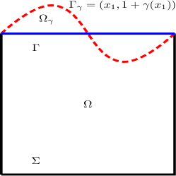
Fig. 1: $\Omega_{\gamma}$ denotes a physical domain with boundary $\partial\Omega_{\gamma}=\Sigma\cup\Gamma_{\gamma}$. Here $\Sigma$ includes the lateral and the bottom boundary and is assumed to be fixed. Furthermore, the top boundary $\Gamma_{\gamma}$ (dotted line) is “free” and is assumed to be a graph of the form $(x_{1},1+\gamma(x_{1}))$, where $\gamma\in{\mathring{W}^{1}_{\infty}\mathinner{\left(0,1\right)}}$ denotes a parametrization. $\Gamma_{\gamma}$ is further mapped to a fixed boundary $\Gamma=(0,1)\times\{1\}$ and in turn the physical domain $\Omega_{\gamma}$ is mapped to a reference domain $\Omega=(0,1)^{2}$, where all computations are carried out.

Of particular interest to us is the control of a model FBP previously studied by P. Saavedra and L. R. Scott in [20] and formulated in graph form; see Figure 1 where the free boundary $\Gamma_{\gamma}$ is the dotted line. The state equations (2b) involve a Laplace equation in the bulk and a Young-Laplace equation on the free boundary to account for surface tension. This amounts to solving a second-order system both in the bulk and on the interface. Below we give a detailed description of the problem.

Let ${\mathring{W}^{1}_{\infty}\mathinner{\left(\text{\rm I}\right)}}$ be the Sobolev space of Lipschitz continuous functions on the unit interval $\text{\rm I}=(0,1)$ which vanish at $0$ and $1$. Let $\gamma\in{\mathring{W}^{1}_{\infty}\mathinner{\left(\text{\rm I}\right)}}$ denote a parametrization of the top boundary (see Figure 1) of the physical domain $\Omega_{\gamma}\subset\Omega^{*}\subset\mathbb{R}^{2}$ with boundary $\partial\Omega_{\gamma}\mathrel{\mathop{\mathchar 58\relax}}=\Gamma_{\gamma}\cup\Sigma$, defined as

$$\Omega^{*} =(0,1)\times(0,2),$$

$${\Omega_{\gamma}} =\mathinner{\left\{(x_{1},x_{2})\,\mathrel{\mathop{\mathchar 58\relax}}\,x_{1}\in\text{\rm I},\;0<x_{2}<1+\gamma(x_{1})\right\}},$$

$$\Gamma_{\gamma} =\mathinner{\left\{(x_{1},x_{2})\,\mathrel{\mathop{\mathchar 58\relax}}\,x_{1}\in\text{\rm I},\;x_{2}=1+\gamma(x_{1})\right\}},$$

$$\Sigma =\partial\Omega_{\gamma}\setminus\Gamma_{\gamma},$$

$$\Gamma =\mathinner{\left\{(x_{1},x_{2})\,\mathrel{\mathop{\mathchar 58\relax}}\,x_{1}\in\text{\rm I},\;x_{2}=1\right\}};$$

$\Omega^{*}$ and $\Sigma$ are fixed while $\Omega_{\gamma}$ and $\Gamma_{\gamma}$ deform according to $\gamma$. Hereafter we will identify $\Gamma$ with I as well as Sobolev spaces defined on them. Since $\gamma$ is Lipschitz continuous with constant $1$, according to (2c), we deduce that $\mathinner{\!\left\lvert\gamma\right\rvert}\leq 1/2$; this guarantees that $\Omega_{\gamma}\subset\Omega^{*}$.

We want to find an optimal control $u\in{\mathcal{U}_{ad}}\subset{L^{2}\mathinner{\left(\text{\rm I}\right)}}$ so that the solution pair $\mathinner{\left(\gamma,y\right)}$ of the FBP approximates a given boundary $\gamma_{d}\mathrel{\mathop{\mathchar 58\relax}}\text{\rm I}\to\mathbb{R}$ and potential $y_{d}\mathrel{\mathop{\mathchar 58\relax}}\Omega^{*}\to\mathbb{R}$. This amounts to solving the problem: minimize

$$\mathcal{J}\mathinner{\left(\gamma,y,u\right)}\mathrel{\mathop{\mathchar 58\relax}}=\frac{1}{2}\mathinner{\!\left\lVert\gamma-\gamma_{d}\right\rVert}_{L^{2}\mathinner{\left(\text{\rm I}\right)}}^{2}+\frac{1}{2}\mathinner{\!\left\lVert y-y_{d}\right\rVert}_{L^{2}\mathinner{\left({\Omega_{\gamma}}\right)}}^{2}+\frac{\lambda}{2}\mathinner{\!\left\lVert u\right\rVert}_{L^{2}\mathinner{\left(\text{\rm I}\right)}}^{2},$$ (2a)

subject to the state equations

$$\left\{\begin{aligned} -\Delta y&=0&&{\textnormal{in }}{\Omega_{\gamma}}\\ y&=v&&{\textnormal{on }}\partial{\Omega_{\gamma}}\\ -\kappa\mathcal{H}\mathinner{\left[\gamma\right]}+{\partial_{\nu}}y\mathinner{\left(\cdot,1+\gamma\right)}&=u&&{\textnormal{on }}\text{\rm I}\\ \gamma(0)=\gamma(1)&=0,\end{aligned}\right.$$ (2b)

the state constraints

$$\mathinner{\!\left\lvert\operatorname{d}\!_{x_{1}}\gamma\right\rvert}\leq 1\quad{\textnormal{a.e. }}\text{\rm I},$$ (2c)

with $$\operatorname{d}\!_{x_{1}} x_{1}$$ being the total derivative with respect to , and the control constraint

$$u \in{\mathcal{U}_{ad}}$$ (2d)

dictated by $${\mathcal{U}_{ad}} {L^{2}\mathinner{\left(\text{\rm I}\right)}}$$, a closed ball in , to be specified later in Definition 5.

Here $\lambda>0$ is a stabilization parameter; $v\in{W^{1}_{p}\mathinner{\left(\Omega^{*}\right)}}$, $p>2$ [20, Lemma 2], is given which in principle could act as a Dirichlet boundary control;

$$\mathcal{H}\mathinner{\left[\gamma\right]}\mathrel{\mathop{\mathchar 58\relax}}=\operatorname{d}\!_{x_{1}}\mathinner{\left(\frac{\operatorname{d}\!_{x_{1}}\gamma}{\sqrt{1+\mathinner{\!\left\lvert\operatorname{d}\!_{x_{1}}\gamma\right\rvert}^{2}}}\right)}$$

is the curvature of $\gamma$; and $\kappa>0$ plays the role of surface tension coefficient.

Optimal control of partial differential equations (PDEs) allows us to achieve a specific goal (2a) with PDE (2b) and other constraints (2c)-(2d) being satisfied and can be highly beneficial in practice (see [23] for more details). For example using the reverse electrowetting, i.e. by applying a control to change the shape of fluid droplets, one can generate enough power to charge a cellphone [15]. There has been various attempts to solve optimal control problems with a FBP constraint. We refer to [12, 13] for control of a two phase Stefan problem in graph formulation and [6] for the same problem in level set formulation. Paper [18] discusses optimal control of a FBP with Stokes flow. Even though problem (2a)-(2d) is relatively simple, it captures the essential features associated with surface tension effects found in more complex systems, and allows us to develop a complete second-order analysis, based on [23], which is absent in the existing literature on FBP.

Depending on the role of the free boundary there are several methodologies to formulate a FBP. We choose the sharp interface method written in graph form (see Figure 1). The (free) interface $\Gamma_{\gamma}$ is governed by the explicit nonlinear PDE

$$-\kappa\mathcal{H}\mathinner{\left[\gamma\right]}+{\partial_{\nu}}y=u.$$

A similar approach was used in [12, 13] for the optimal control of a Stefan problem, but without the full accompanying theory developed herein. Alternative approaches to treat FBPs are the level set method and the diffuse interface method [8, 6].

We use a fixed domain approach to solve the optimal control free boundary problem (OC-FBP). In fact, we transform $\Omega_{\gamma}$ to $\Omega=(0,1)^{2}$ and $\Gamma_{\gamma}$ to $\Gamma=(0,1)\times\mathinner{\left\{1\right\}}$ (see Figure 1), at the expense of having a governing PDE with rough coefficients. This avoids dealing with shape sensitivity analysis [21, 9]. We refer to [24] for a comparison between these approaches applied to a FBP. Using operator interpolation [22] we demonstrate how to improve the existing regularity of state variables derived earlier in [20], which turns out to be instrumental to derive the second-order sufficient condition.

One of the challenges of an OC-FBP is dealing with possible topological changes of the domain by introducing state constraints. Our analysis provides control constraints which always enforce the state constraints, i.e. we can simply treat OC-FBP as a control constrained problem without any state constraints. We refer to [23, Section 6.2] and references therein for state and gradient constraints problems along with the associated difficulties. We will provide a comprehensive numerical approach for the control problem (2) in a forthcoming paper [5].

We have organized this paper as follows. A detailed problem description on a fixed domain is given in section 2. We introduce the Lagrangian functional to formally derive the first-order necessary optimality conditions in section 3. We present a rigorous justification of the Lagrangian results in the remaining sections. To this end, we introduce a control-to-state operator in section 4 and show that for a particular set of admissible controls it is twice Fréchet differentiable. Finally, we write the optimal control problem in its reduced form and show the existence of a control under slightly higher regularity together with second-order sufficient conditions in section 5.

2 OC-FBP on Reference Domain

We start by mapping the physical domain $\Omega_{\gamma}$ onto the fixed reference domain $\Omega=\mathinner{\left(0,1\right)}^{2}$. This results in an optimal control problem subject to PDE constraints with nonlinear coefficients depending on $\gamma$ but without an explicit interface. The idea is to map the unknown domain ${\Omega_{\gamma}}$ onto the fixed domain $\Omega$ using the inverse of the Lipschitz map $\Psi\mathrel{\mathop{\mathchar 58\relax}}\Omega\to{\Omega_{\gamma}}$ defined as

$$\Psi(x_{1},x_{2})=\mathinner{\left(x_{1},\mathinner{\left(1+\gamma\mathinner{\left(x_{1}\right)}\right)}x_{2}\right)}\in{\Omega_{\gamma}},\quad{\textnormal{for }}\mathinner{\left(x_{1},x_{2}\right)}\in\Omega.$$ (3)

Since $\gamma$ is Lipschitz continuous with constant $1$, according to (2c), we deduce that $\mathinner{\!\left\lvert\gamma\right\rvert}\leq 1/2$ and that $\Psi$ is invertible because its Jacobian is $J_{\gamma}=1+\gamma$. Furthermore, the inverse of $\Psi$ is also Lipschitz. Moreover, it becomes routine to check that the Laplace equation $\Delta y=0$ in ${\Omega_{\gamma}}$ and ${\partial_{\nu}}y$ on $\Gamma_{\gamma}$ can be written as

$$\operatorname{div}\mathinner{\left(A\mathinner{\left[\gamma\right]}\nabla y\right)}=0\quad\mbox{in }\Omega,\qquad A\mathinner{\left[\gamma\right]}\nabla y\cdot\nu\mathinner{\left(1+\mathinner{\!\left\lvert\operatorname{d}\!_{x_{1}}\gamma\right\rvert}^{2}\right)}^{-1/2}\quad\mbox{on }\text{\rm I},$$

where $\nu=\mathinner{\left[0,1\right]}^{T}$, and $A\mathrel{\mathop{\mathchar 58\relax}}{\mathring{W}^{1}_{\infty}\mathinner{\left(\text{\rm I}\right)}}\rightarrow L^{\infty}(\Omega)^{2\times 2}$ is the Nemytskii operator [23, Chapter 4] defined by

$$A\mathinner{\left[\gamma\right]} =\begin{bmatrix}1+\gamma(x_{1})&-\operatorname{d}\!_{x_{1}}\gamma(x_{1})x_{2}\\ -\operatorname{d}\!_{x_{1}}\gamma(x_{1})x_{2}&\frac{1+\mathinner{\left(\operatorname{d}\!_{x_{1}}\gamma(x_{1})x_{2}\right)}^{2}}{1+\gamma(x_{1})}\end{bmatrix}.$$ (4)

It is convenient to write $A_{2,2}\mathinner{\left[\gamma\right]}$ as $\Phi\mathinner{\left[\gamma\right]}\mathrel{\mathop{\mathchar 58\relax}}=\varphi\mathinner{\left(\gamma(x_{1}),\operatorname{d}\!_{x_{1}}\gamma(x_{1})x_{2}\right)}$, where $\varphi\mathinner{\left(a,b\right)}\mathrel{\mathop{\mathchar 58\relax}}=\mathinner{\left(1+b^{2}\right)}/\mathinner{\left(1+a\right)}.$

We simplify the exposition by exploiting the fact that we are only interested in small ${\mathring{W}^{1}_{\infty}\mathinner{\left(\text{\rm I}\right)}}$-perturbations of the flat case $\gamma=0$, namely we have $\operatorname{d}\!_{x_{1}}\gamma$ small pointwise. We thus make the following assumptions:

• Linearized curvature: $\mathcal{H}_{lin}\mathinner{\left[\gamma\right]}={\operatorname{d}\!^{2}_{x_{1}}\gamma}\mathinner{\left(1+\mathinner{\!\left\lvert\operatorname{d}\!_{x_{1}}\gamma\right\rvert}^{2}\right)}^{-1/2}$.

• Scaled control: $u$ becomes $u\mathinner{\left(1+\mathinner{\!\left\lvert\operatorname{d}\!_{x_{1}}\gamma\right\rvert}^{2}\right)}^{-1/2}$.

These assumptions are not crucial. The nonlinear curvature $\mathcal{H}[\gamma]$ formally reads

$$\mathcal{H}[\gamma]=\operatorname{d}\!_{x_{1}}\mathinner{\left(\frac{\operatorname{d}\!_{x_{1}}\gamma}{\sqrt{1+\mathinner{\!\left\lvert\operatorname{d}\!_{x_{1}}\gamma\right\rvert}^{2}}}\right)}=\frac{\operatorname{d}\!_{x_{1}}^{2}\gamma}{\mathinner{\left(1+\mathinner{\!\left\lvert\operatorname{d}\!_{x_{1}}\gamma\right\rvert}^{2}\right)}^{3/2}},$$

which is similar to the linearized curvature $\mathcal{H}_{lin}$ except for the $L^{\infty}(\text{\rm I})$ factor $1/(1+\mathinner{\!\left\lvert\operatorname{d}\!_{x_{1}}\gamma\right\rvert}^{2})\approx 1$. Assumption ${\bf(A_{1})}$ simplifies the structure of the bilinear form $\mathcal{B}_{\Gamma}$ in (21). On the other hand, the scaling of the control in ${\bf(A_{2})}$ avoids unnecessarily complicating the right-hand-side of (5b) below, which would contain $u\mathinner{\left(1+\mathinner{\!\left\lvert\operatorname{d}\!_{x_{1}}\gamma\right\rvert}^{2}\right)}^{1/2}$ instead of simply $u$. Our analysis below extends to the general setting without assumptions ${\bf(A_{1})}$ and ${\bf(A_{2})}$.

Under these assumptions and applying the map $\Psi$, the optimal control problem (2) becomes: minimize

$$\mathcal{J}\mathinner{\left(\gamma,y,u\right)}\mathrel{\mathop{\mathchar 58\relax}}=\frac{1}{2}\mathinner{\!\left\lVert\gamma-\gamma_{d}\right\rVert}_{L^{2}\mathinner{\left(\text{\rm I}\right)}}^{2}+\frac{1}{2}\mathinner{\!\left\lVert\mathinner{\left(y+v-y_{d}\right)}\sqrt{J_{\gamma}}\right\rVert}_{L^{2}\mathinner{\left(\Omega\right)}}^{2}+\frac{\lambda}{2}\mathinner{\!\left\lVert u\right\rVert}_{L^{2}\mathinner{\left(\text{\rm I}\right)}}^{2}$$ (5a)

subject to the state equations $$\mathinner{\left(\gamma,y\right)}\in{\mathring{W}^{1}_{\infty}\mathinner{\left(\text{\rm I}\right)}}\times{\mathring{W}^{1}_{p}\mathinner{\left(\Omega\right)}}$$

$$\left\{\begin{aligned} -\operatorname{div}\mathinner{\left(A\mathinner{\left[\gamma\right]}\nabla\mathinner{\left(y+v\right)}\right)}&=0&&{\textnormal{in }}\Omega\\ -\kappa\operatorname{d}\!_{x_{1}}^{2}\gamma+A\mathinner{\left[\gamma\right]}\nabla\mathinner{\left(y+v\right)}\cdot\nu&=u&&{\textnormal{in }}\text{\rm I}\\ \end{aligned}\right.$$ (5b)

the state constraints

$$\mathinner{\!\left\lvert\operatorname{d}\!_{x_{1}}\gamma\right\rvert}\leq 1\quad{\textnormal{a.e. }}\text{\rm I},$$ (5c)

with $$\operatorname{d}\!_{x_{1}} x_{1}$$ being the total derivative with respect to , and the control constraint

$$u \in{\mathcal{U}_{ad}}$$ (5d)

dictated by $${\mathcal{U}_{ad}} {L^{2}\mathinner{\left(I\right)}}$$, a closed ball in , to be specified later in Definition 5.

In order to derive the first- and second-order optimality conditions in later sections, we need to compute the first- and second-order directional derivatives of $A$, which in turn requires computing the directional derivative of the Nemytskii operator $\Phi$ defined above. To simplify notation, we drop the evaluation of $\gamma$ and $\operatorname{d}\!_{x_{1}}\gamma$ at $x_{1}$. The derivative of $\Phi$ in the direction $h$ at $(\gamma,x_{2}\operatorname{d}\!_{x_{1}}\gamma)$ is given by

$$\operatorname{D\!}\Phi\mathinner{\left[\gamma\right]}\langle h\rangle=\partial_{a}\varphi\mathinner{\left(\gamma,x_{2}\operatorname{d}\!_{x_{1}}\gamma\right)}h+\partial_{b}\varphi\mathinner{\left(\gamma,x_{2}\operatorname{d}\!_{x_{1}}\gamma\right)}x_{2}\operatorname{d}\!_{x_{1}}h$$

where

$$\nabla\varphi(a,b) \mathrel{\mathop{\mathchar 58\relax}}=\begin{bmatrix}\partial_{a}\varphi(a,b)&\partial_{b}\varphi(a,b)\end{bmatrix}=\begin{bmatrix}-\frac{1+b^{2}}{(1+a)^{2}}&\frac{2b}{1+a}\end{bmatrix}.$$

Furthermore, we obtain the following representation for $\operatorname{D\!}A$ in terms of $h$ and $\operatorname{d}\!_{x_{1}}h$

$$\operatorname{D\!}A\mathinner{\left[\gamma\right]}\langle h\rangle \mathrel{\mathop{\mathchar 58\relax}}=A_{1}\mathinner{\left[\gamma\right]}h+A_{2}\mathinner{\left[\gamma\right]}\operatorname{d}\!_{x_{1}}h$$

$$~{}=\begin{bmatrix}1&0\\ 0&\partial_{a}\varphi\mathinner{\left(\gamma,x_{2}\operatorname{d}\!_{x_{1}}\gamma\right)}\end{bmatrix}h+\begin{bmatrix}0&-x_{2}\\ -x_{2}&x_{2}\partial_{b}\varphi\mathinner{\left(\gamma,x_{2}\operatorname{d}\!_{x_{1}}\gamma\right)}\end{bmatrix}\operatorname{d}\!_{x_{1}}h,$$ (6)

whence the remainder $\mathfrak{R}_{A}\mathinner{\left[\gamma,h\right]}$ at $\gamma$ in the direction $h$ reads

$$\mathfrak{R}_{A}\mathinner{\left[\gamma,h\right]}\mathrel{\mathop{\mathchar 58\relax}}=A\mathinner{\left[\gamma+h\right]}-A\mathinner{\left[\gamma\right]}-\operatorname{D\!}A\mathinner{\left[\gamma\right]}\langle h\rangle$$ (7a)

and

$$\lim_{\mathinner{\!\left\lvert h\right\rvert}_{W^{1}_{\infty}\mathinner{\left(\text{\rm I}\right)}}\to 0}\frac{\mathinner{\!\left\lVert\mathfrak{R}_{A}\mathinner{\left[\gamma,h\right]}\right\rVert}_{L^{\infty}\mathinner{\left(\Omega\right)}}}{\mathinner{\!\left\lvert h\right\rvert}_{W^{1}_{\infty}\mathinner{\left(\text{\rm I}\right)}}}=0;$$ (7b)

(7b) follows directly from the structure of $$A$$ [23, Lemma 4.12].

The Hessian of $\varphi$ is

$$\nabla^{2}\varphi(a,b) =\begin{bmatrix}\partial_{a}^{2}\varphi(a,b)&\partial_{ab}\varphi(a,b)\\ \partial_{ba}\varphi(a,b)&\partial_{b}^{2}\varphi(a,b)\end{bmatrix}=2\begin{bmatrix}\frac{1+b^{2}}{(1+a)^{3}}&\frac{-b}{(1+a)^{2}}\\ \frac{-b}{(1+a)^{2}}&\frac{1}{1+a}\end{bmatrix}.$$

The second-order derivative of $\Phi$ in the direction $h_{1}$ followed by $h_{2}$ evaluated at $(\gamma,x_{2}\operatorname{d}\!_{x_{1}}\gamma)$ is

$$\operatorname{D\!}^{2}\Phi\mathinner{\left[\gamma\right]}\langle h_{2},h_{1}\rangle =\partial_{a}^{2}\varphi\mathinner{\left(\gamma,x_{2}\operatorname{d}\!_{x_{1}}\gamma\right)}h_{2}h_{1}+\partial_{ab}\varphi\mathinner{\left(\gamma,x_{2}\operatorname{d}\!_{x_{1}}\gamma\right)}x_{2}h_{2}\operatorname{d}\!_{x_{1}}h_{1}$$

$$\quad+\partial_{ab}\varphi\mathinner{\left(\gamma,x_{2}\operatorname{d}\!_{x_{1}}\gamma\right)}x_{2}\operatorname{d}\!_{x_{1}}h_{2}h_{1}+\partial_{b}^{2}\varphi\mathinner{\left(\gamma,x_{2}\operatorname{d}\!_{x_{1}}\gamma\right)}x_{2}^{2}\operatorname{d}\!_{x_{1}}h_{2}\operatorname{d}\!_{x_{1}}h_{1}.$$

Finally, we obtain the following representation for $\operatorname{D\!}^{2}\!\!A$ in terms of $h_{1}$ and $h_{2}$

$$\operatorname{D\!}^{2}\!\!A\mathinner{\left[\gamma\right]}\langle h_{2},h_{1}\rangle=\begin{bmatrix}0&0\\ 0&\operatorname{D\!}^{2}\Phi\mathinner{\left[\gamma\right]}\langle h_{2},h_{1}\rangle\end{bmatrix},$$ (8)

whence the remainder $\mathfrak{R}_{\operatorname{D\!}A}\mathinner{\left[\gamma,h_{1},h_{2}\right]}$ at $\gamma$ reads

$$\mathfrak{R}_{\operatorname{D\!}A}\mathinner{\left[\gamma,h_{1},h_{2}\right]}\mathrel{\mathop{\mathchar 58\relax}}=\operatorname{D\!}A\mathinner{\left[\gamma+h_{2}\right]}\langle h_{1}\rangle-\operatorname{D\!}A\mathinner{\left[\gamma\right]}\langle h_{1}\rangle-\operatorname{D\!}^{2}\!\!A\mathinner{\left[\gamma\right]}\langle h_{1},h_{2}\rangle,$$ (9a)

and [23, Lemma 4.12]

$$\lim_{\begin{subarray}{c}\mathinner{\!\left\lvert h_{1}\right\rvert}_{W^{1}_{\infty}\mathinner{\left(\text{\rm I}\right)}}\to 0\\ \mathinner{\!\left\lvert h_{2}\right\rvert}_{W^{1}_{\infty}\mathinner{\left(\text{\rm I}\right)}}\to 0\end{subarray}}\frac{\mathinner{\!\left\lVert\mathfrak{R}_{\operatorname{D\!}A}\mathinner{\left[\gamma,h_{1},h_{2}\right]}\right\rVert}_{L^{\infty}(\Omega)^{2\times 2}}}{\mathinner{\!\left\lvert h_{1}\right\rvert}_{W^{1}_{\infty}\mathinner{\left(\text{\rm I}\right)}}\mathinner{\!\left\lvert h_{2}\right\rvert}_{W^{1}_{\infty}\mathinner{\left(\text{\rm I}\right)}}}=0.$$ (9b)

Proposition 1 (bounds on $A$).

If the state constraint (5c) holds, then there exists a positive constant $C_{A}<\infty$ such that

$$\mathinner{\!\left\lVert A\mathinner{\left[\gamma\right]}\right\rVert}_{L^{\infty}\mathinner{\left(\Omega\right)}^{2\times 2}} +\sup_{\mathinner{\!\left\lvert h\right\rvert}_{W^{1}_{\infty}\mathinner{\left(\text{\rm I}\right)}}=1}\mathinner{\!\left\lVert\operatorname{D\!}A\mathinner{\left[\gamma\right]}\langle h\rangle\right\rVert}_{L^{\infty}\mathinner{\left(\Omega\right)}^{2\times 2}}$$ (10)

$$+\sup_{\begin{subarray}{c}\mathinner{\!\left\lvert h_{1}\right\rvert}_{W^{1}_{\infty}\mathinner{\left(\text{\rm I}\right)}}=1\\ \mathinner{\!\left\lvert h_{2}\right\rvert}_{W^{1}_{\infty}\mathinner{\left(\text{\rm I}\right)}}=1\end{subarray}}\mathinner{\!\left\lVert\operatorname{D\!}^{2}\!\!A\mathinner{\left[\gamma\right]}\langle h_{1},h_{2}\rangle\right\rVert}_{L^{\infty}\mathinner{\left(\Omega\right)}^{2\times 2}}\leq C_{A}.$$

3 Formal Lagrangian Formulation

In this section we formally derive the first-order necessary optimality conditions using the Lagrangian approach described in [23]. To this end, we will assume that the admissible control set ${\mathcal{U}_{ad}}$ guarantees the state constraints (5c), a pending issue we revisit and examine in detail in section 4. For a rigorous analysis of the existence of Lagrange multipliers in Banach spaces we refer to [27].

It is well known that for a convex optimal control problem with linear constraints, the first-order necessary optimality conditions are also sufficient conditions [23, Lemma 2.21]. This does not apply to our problem because, despite linearizing the curvature via assumption $(\bf A_{1})$, the state equations (5b) are still highly nonlinear and the optimization nonconvex. We will derive the second-order sufficient optimality conditions in section 5.

Let $s,r$ denote the adjoint variables corresponding to states $\gamma,y$ respectively. Then the formal Lagrangian functional is given by

$$\mathcal{L}(\gamma,y,u,r,s)\mathrel{\mathop{\mathchar 58\relax}}=\mathcal{J}\mathinner{\left(\gamma,y,u\right)} +\int_{\Omega}\operatorname{div}\mathinner{\left(A\mathinner{\left[\gamma\right]}\nabla\mathinner{\left(y+v\right)}\right)}r\operatorname{d\!}x$$ (11)

$$+\int_{0}^{1}\mathinner{\left(\kappa\operatorname{d}\!^{2}_{x_{1}}\gamma-A\mathinner{\left[\gamma\right]}\nabla\mathinner{\left(y+v\right)}\cdot\nu+u\right)}s\operatorname{d\!}\sigma;$$

we implicitly assume regularity in writing (11). Additionally, if $\mathinner{\left(\bar{\gamma},\bar{y},\bar{u},\bar{r},\bar{s}\right)}$ is a critical point for $\mathcal{L}$, then the first-order necessary optimality conditions are

$$\left\langle\operatorname{D\!}_{v}\mathcal{L}{\mathinner{\left(\bar{\gamma},\bar{y},\bar{u},\bar{r},\bar{s}\right)}},h\right\rangle_{\mathbb{V}^{*},\mathbb{V}} =0\qquad\forall h\in\mathbb{V},$$ (12a)

$${\mathop{\left\langle\operatorname{D\!}_{u}\mathcal{L}{\mathinner{\left(\bar{\gamma},\bar{y},\bar{u},\bar{r},\bar{s}\right)}},u-\bar{u}\right\rangle}}_{{L^{2}\mathinner{\left(\text{\rm I}\right)}}\times{L^{2}\mathinner{\left(\text{\rm I}\right)}}} \geq 0\qquad\forall u\in\mathcal{U}_{ad},$$ (12b)

where

$$\mathinner{\left(v,\mathbb{V}\right)}\in\mathinner{\left\{\mathinner{\left(\gamma,{\mathring{W}^{1}_{\infty}\mathinner{\left(\text{\rm I}\right)}}\right)},\mathinner{\left(y,{\mathring{W}^{1}_{p}\mathinner{\left(\Omega\right)}}\right)},\mathinner{\left(r,{\mathring{W}^{1}_{q}\mathinner{\left(\Omega\right)}}\right)},\mathinner{\left(s,{\mathring{W}^{1}_{1}\mathinner{\left(\text{\rm I}\right)}}\right)}\right\}},$$ (12c)

$p,q$ are Hölder conjugate indices, i.e. $1/p+1/q=1$, with $p>2$, and $\left\langle\cdot,\cdot\right\rangle_{\mathbb{V}^{*},\mathbb{V}}$ stands for duality pairings. Therefore, computing $\mathinner{\left(\bar{\gamma},\bar{y},\bar{u},\bar{r},\bar{s}\right)}$ requires solving the nonlinear system (12). We again point out that the calculations in this section are merely formal and the functions in (12c) will be justified later in sections 4 and 5. In practice this can be realized using techniques described in [4, 14, 23]. For variational inequalities of the first kind, such as (12b), we refer to [11] for relaxation and augmented Lagrangian techniques and to [7] for semi-smooth Newton methods. The remainder of this section is devoted to the derivation of the equations satisfied by $\mathinner{\left(\bar{\gamma},\bar{y},\bar{u},\bar{r},\bar{s}\right)}$ using the nonlinear system above.

Since $\left\langle\operatorname{D\!}_{\mathinner{\left\{s,r\right\}}}\mathcal{L}{\mathinner{\left(\bar{\gamma},\bar{y},\bar{u},\bar{r},\bar{s}\right)}},h\right\rangle=0$ implies that $(\bar{\gamma},\bar{y})$ solves the state equations (5b), we focus on the adjoint equations $\left\langle\operatorname{D\!}_{\mathinner{\left\{\gamma,y\right\}}}\mathcal{L}{\mathinner{\left(\bar{\gamma},\bar{y},\bar{u},\bar{r},\bar{s}\right)}},h\right\rangle=0$. Using Green’s theorem and assuming smoothness, the formal Lagrangian $\mathcal{L}$ can be rewritten as:

$$\mathcal{L}(y, \gamma,u,r,s)=\mathcal{J}\mathinner{\left(\gamma,y,u\right)}+\int_{\Omega}\operatorname{div}\mathinner{\left(A\mathinner{\left[\gamma\right]}\nabla r\right)}\mathinner{\left(y+v\right)}\operatorname{d\!}x$$ (13)

$$\quad+\int_{\partial\Omega}\mathinner{\left(rA\mathinner{\left[\gamma\right]}\nabla\mathinner{\left(y+v\right)}-\mathinner{\left(y+v\right)}A\mathinner{\left[\gamma\right]}\nabla r\right)}\cdot\nu\operatorname{d\!}\sigma$$

$$\quad+\int_{0}^{1}\mathinner{\left(\kappa\gamma\operatorname{d}\!^{2}_{x_{1}}s-sA\mathinner{\left[\gamma\right]}\nabla\mathinner{\left(y+v\right)}\cdot\nu+us\right)}\operatorname{d\!}\sigma+{\kappa\mathinner{\left(\operatorname{d}\!_{x_{1}}\gamma s-\gamma\operatorname{d}\!_{x_{1}}s\right)}}\bigg{|}_{0}^{1}.$$

Imposing $\left\langle\operatorname{D\!}_{y}\mathcal{L}{\mathinner{\left(\bar{\gamma},\bar{y},\bar{u},\bar{r},\bar{s}\right)}},h\right\rangle=0$ to (13) implies that for every $h\in{\mathring{W}^{1}_{p}\mathinner{\left(\Omega\right)}}$

$$-\int_{\Omega}\operatorname{div}\mathinner{\left(A\mathinner{\left[\bar{\gamma}\right]}\nabla\bar{r}\right)}h\operatorname{d\!}x =\int_{\Omega}\mathinner{\left(\bar{y}+v-y_{d}\right)}\mathinner{\left(1+\bar{\gamma}\right)}h\operatorname{d\!}x$$ (14a)

$$\quad+\int_{\partial\Omega}\bar{r}A\mathinner{\left[\bar{\gamma}\right]}\nabla h\cdot\nu\operatorname{d\!}\sigma-\int_{0}^{1}\bar{s}A\mathinner{\left[\bar{\gamma}\right]}\nabla h\cdot\nu\operatorname{d\!}\sigma.$$

Next, without loss of generality ($$C_{0}^{\infty}\mathinner{\left(\Omega\right)} {\mathring{W}^{1}_{p}\mathinner{\left(\Omega\right)}}$$ is dense in ), we obtain

$$-\int_{\Omega}\operatorname{div}\mathinner{\left(A\mathinner{\left[\bar{\gamma}\right]}\nabla\bar{r}\right)}h\operatorname{d\!}x =\int_{\Omega}\mathinner{\left(\bar{y}+v-y_{d}\right)}\mathinner{\left(1+\bar{\gamma}\right)}h\operatorname{d\!}x \forall h\in C_{0}^{\infty}\mathinner{\left(\Omega\right)},$$ (14b)

whereas, using that $$A\mathinner{\left[\gamma\right]}\nabla h\cdot\nu \partial\Omega$$ can be chosen arbitrarily on we deduce from (14a) and (14b) that

$$\bar{r}-\bar{s}|_{\Gamma}=0,\qquad\bar{r}|_{\Sigma}=0.$$ (14c)

In view of (14b-c), the strong form of the boundary value problem for $\bar{r}$ is: seek $\bar{r}\in{W^{1}_{q}\mathinner{\left(\Omega\right)}}$ such that

$$\left\{\begin{aligned} -\operatorname{div}\mathinner{\left(A\mathinner{\left[\bar{\gamma}\right]}\nabla\bar{r}\right)}&=\mathinner{\left(\bar{y}+v-y_{d}\right)}\mathinner{\left(1+\bar{\gamma}\right)}&&{\textnormal{in }}\Omega\\ \bar{r}&=\bar{s}&&{\textnormal{on }}\Gamma\\ \bar{r}&=0&&{\textnormal{on }}\Sigma.\end{aligned}\right.$$ (15)

Next we employ the same technique to obtain the equations for the second adjoint variable $\bar{s}$: we impose $\left\langle\operatorname{D\!}_{\gamma}\mathcal{L}{\mathinner{\left(\bar{\gamma},\bar{y},\bar{u},\bar{r},\bar{s}\right)}},h\right\rangle=0$ to (13) and make use of the boundary conditions in (15) to obtain for every $h\in{\mathring{W}^{1}_{\infty}\mathinner{\left(\text{\rm I}\right)}}$

$$-\int_{0}^{1}\kappa\operatorname{d}\!^{2}_{x_{1}}sh\operatorname{d\!}\sigma =\int_{0}^{1}\mathinner{\left(\bar{\gamma}-\gamma_{d}\right)}h\operatorname{d\!}\sigma$$

$$\quad+\frac{1}{2}\int_{\Omega}\mathinner{\!\left\lvert\bar{y}+v-y_{d}\right\rvert}^{2}h\operatorname{d\!}x-\int_{\Omega}\operatorname{D\!}A\mathinner{\left[\bar{\gamma}\right]}\langle h\rangle\nabla\mathinner{\left(\bar{y}+v\right)}\cdot\nabla\bar{r}\operatorname{d\!}x.$$

Therefore, the strong form of the boundary value problem for $\bar{s}$ is: seek $\bar{s}\in{\mathring{W}^{1}_{1}\mathinner{\left({\text{\rm I}}\right)}}$

$$\left\{\begin{aligned} -\kappa\operatorname{d}\!^{2}_{x_{1}}\bar{s}&=\mathinner{\left(\bar{\gamma}-\gamma_{d}\right)}+\frac{1}{2}\int_{0}^{1}\mathinner{\!\left\lvert\bar{y}+v-y_{d}\right\rvert}^{2}\operatorname{d\!}x_{2}-\int_{0}^{1}A_{1}\mathinner{\left[\bar{\gamma}\right]}\nabla\mathinner{\left(\bar{y}+v\right)}\cdot\nabla\bar{r}\operatorname{d\!}x_{2}\\ &\quad+\operatorname{d}\!_{x_{1}}\mathinner{\left(\int_{0}^{1}A_{2}\mathinner{\left[\bar{\gamma}\right]}\nabla\mathinner{\left(\bar{y}+v\right)}\cdot\nabla\bar{r}\operatorname{d\!}x_{2}\right)}\quad{\textnormal{in }}\text{\rm I}\\ \bar{s}(0)&=\bar{s}(1)=0,\end{aligned}\right.$$ (16)

where $A_{1},A_{2}$ denote the representation of $DA$ given in (2). We note that the integrals on the right hand side of (16) correspond to integration in $x_{2}$ (vertical) direction.

Finally, (12b) implies

$${\mathop{\left\langle\lambda\bar{u}+\bar{s},u-\bar{u}\right\rangle}}_{{L^{2}\mathinner{\left(\text{\rm I}\right)}}\times{L^{2}\mathinner{\left(\text{\rm I}\right)}}}\geq 0,\qquad\forall u\in\mathcal{U}_{ad}.$$ (17)

To summarize, the solution $\mathinner{\left(\bar{\gamma},\bar{y},\bar{u},\bar{r},\bar{s}\right)}$ to the first-order optimality system (12) satisfies (5b), (15), (16) and (17). We stress that the formal approach presented in this section is very systematic and highly useful even though it is not clear at the moment how to show the existence and (local) uniqueness of the optimal control $\bar{u}$. A rigorous analysis will be developed in the next two sections.

4 The Control-to-state Map $G_{v}$

Let $G_{v}$ denote the nonlinear map

$$\begin{array}[]{ccrcl}{G_{v}}&\colon&{\mathcal{U}}&\longrightarrow&{\mathbb{W}^{1}}\\ \mbox{}&\mbox{}&{u}&\longmapsto&{\mathinner{\left(\gamma,y\right)}}\end{array},$$ (20)

where $\mathbb{W}^{1}\mathrel{\mathop{\mathchar 58\relax}}={\mathring{W}^{1}_{\infty}\mathinner{\left(\text{\rm I}\right)}}\times{\mathring{W}^{1}_{p}\mathinner{\left(\Omega\right)}}$, $(\gamma,y)$ solves (5b), and the subscript on $G_{v}$ denotes dependence on a fixed and non-trivial $v\in{W^{1}_{p}\mathinner{\left(\Omega\right)}}$. Furthermore, $\mathcal{U}\subset L^{2}(\text{\rm I})$ is an open ball containing the set of admissible controls ${\mathcal{U}_{ad}}$,

$${\mathcal{U}_{ad}}\subset\mathcal{U}\subset L^{2}(\text{\rm I}),$$

which will be precisely specified in Definition 5. Our goal is to show the existence of a control, derive the first-order necessary and second-order sufficient optimality conditions within the realm of a rigorous mathematical framework. The first-order optimality conditions requires to show that $G_{v}$ is Fréchet differentiable (subsection 4.3) and the second order conditions require $G_{v}$ to be twice Fréchet differentiable (subsection 4.4).

The steps described above are standard for PDE-constrained optimization in fixed domains [23], but our analysis for the linearized curvature OC-FBP is novel. The novelty resides in the highly nonlinear structure of the underlying FBP, which is posed in a pair of Banach spaces one being non-reflexive, and yet we deal with minimal regularity. A number of other control problems for FBPs fall under a similar functional framework [1, 2], but their theory is not as complete and conclusive as ours. This appears to be an area of intense current research.

The first step in this voyage is to show that there exists a unique weak solution to (5b), which implies that $G_{v}$ is a well defined one-to-one nonlinear operator. In fact, it is known [20] that for $u=0$ and $v$ small, a fixed point argument asserts the existence and uniqueness of a weak solution $\mathinner{\left(\gamma,y\right)}$ in $\mathbb{W}^{1}$ to (5b). We further extend this analysis to the case where $u\neq 0$. This gives us an open ball $\mathcal{U}\subset{L^{2}\mathinner{\left(\text{\rm I}\right)}}$ where we can show the existence of solution to (5b).

4.1 Well-posedness of the State System (5b)

The weak form of the system (5b) is: find $(\gamma,y)\in\mathbb{W}^{1}$ such that

$$\left\{\begin{aligned} \mathcal{B}_{\Omega}\mathinner{\left[y+v,z;A\mathinner{\left[\gamma\right]}\right]}&=0&&\forall z\in{\mathring{W}^{1}_{q}\mathinner{\left(\Omega\right)}}\\ \mathcal{B}_{\Gamma}\mathinner{\left[\gamma,\zeta\right]}+\mathcal{B}_{\Omega}\mathinner{\left[y+v,E\zeta;A\mathinner{\left[\gamma\right]}\right]}&={\mathop{\left\langle u,\zeta\right\rangle}}_{{W^{-1}_{\infty}\mathinner{\left(\text{\rm I}\right)}}\times{\mathring{W}^{1}_{1}\mathinner{\left(\text{\rm I}\right)}}}&&\forall\zeta\in{\mathring{W}^{1}_{1}\mathinner{\left(\text{\rm I}\right)}},\end{aligned}\right.$$ (21)

where $\mathcal{B}_{\Gamma}\mathrel{\mathop{\mathchar 58\relax}}{\mathring{W}^{1}_{\infty}\mathinner{\left(\text{\rm I}\right)}}\times{\mathring{W}^{1}_{1}\mathinner{\left(\text{\rm I}\right)}}\to\mathbb{R}$, $\mathcal{B}_{\Omega}\mathrel{\mathop{\mathchar 58\relax}}{\mathring{W}^{1}_{p}\mathinner{\left(\Omega\right)}}\times{\mathring{W}^{1}_{q}\mathinner{\left(\Omega\right)}}\to\mathbb{R}$ are defined by

$$\mathcal{B}_{\Gamma}\mathinner{\left[\gamma,\zeta\right]} \mathrel{\mathop{\mathchar 58\relax}}=\kappa\int_{0}^{1}{\operatorname{d}\!_{x_{1}}\gamma}(x_{1}){\operatorname{d}\!_{x_{1}}\zeta}(x_{1})\operatorname{d\!}x_{1},$$ (22)

$$\mathcal{B}_{\Omega}\mathinner{\left[y,z;A\mathinner{\left[\gamma\right]}\right]} \mathrel{\mathop{\mathchar 58\relax}}=\int_{\Omega}A\mathinner{\left[\gamma\right]}\nabla y\cdot\nabla z\operatorname{d\!}x.$$

Furthermore, $E\mathrel{\mathop{\mathchar 58\relax}}{\mathring{W}^{1}_{1}\mathinner{\left(\text{\rm I}\right)}}\rightarrow{W^{1}_{q}\mathinner{\left(\Omega\right)}}$, $1<q<2$ denotes a continuous extension such that $E\zeta|_{\Gamma}=\zeta$, $E\zeta|_{\Sigma}=0$. In particular, this implies the existence of a constant $C_{E}\geq 1$, which dependes on $\Omega$ and $q$ and blows up as $q$ approaches 2 [20, Lemma 2], such that

$$\mathinner{\!\left\lvert E\zeta\right\rvert}_{W^{1}_{q}\mathinner{\left(\Omega\right)}} \leq C_{E}\mathinner{\!\left\lvert\zeta\right\rvert}_{W^{1}_{1}\mathinner{\left(\text{\rm I}\right)}},\quad\forall\zeta\in{\mathring{W}^{1}_{1}\mathinner{\left(\text{\rm I}\right)}}.$$ (23)

Moreover, when $u\in\mathcal{U}\subset{L^{2}\mathinner{\left(\text{\rm I}\right)}}$ and the test function $\zeta\in{\mathring{W}^{1}_{1}\mathinner{\left(\text{\rm I}\right)}}$, then $\zeta\in L^{2}(\text{\rm I})$ and we may write

$${\mathop{\left\langle u,\zeta\right\rangle}}_{{W^{-1}_{\infty}\mathinner{\left(\text{\rm I}\right)}}\times{\mathring{W}^{1}_{1}\mathinner{\left(\text{\rm I}\right)}}}=\int_{0}^{1}u\zeta,$$ (24)

where ${W^{-1}_{\infty}\mathinner{\left(\text{\rm I}\right)}}$ is the dual space of ${\mathring{W}^{1}_{1}\mathinner{\left(\text{\rm I}\right)}}$; we refer to [3]. Since $\|\zeta\|_{L^{\infty}(\text{\rm I})}\leq|\zeta|_{{\mathring{W}^{1}_{1}\mathinner{\left(\text{\rm I}\right)}}}$, this also enables us to deduce that for $u\in{L^{2}\mathinner{\left(\text{\rm I}\right)}}$

$$\mathinner{\!\left\lVert u\right\rVert}_{W^{-1}_{\infty}\mathinner{\left(\text{\rm I}\right)}}\leq\mathinner{\!\left\lVert u\right\rVert}_{L^{2}\mathinner{\left(\text{\rm I}\right)}}.$$ (25)

We will make use of these two facts repeatedly throughout the rest of the paper.

Proposition 2 ($\inf$-$\sup$ conditions).

The following conditions hold for the bilinear forms $\mathcal{B}_{\Gamma}\mathinner{\left[\cdot,\cdot\right]}$ and $\mathcal{B}_{\Omega}\mathinner{\left[\cdot,\cdot;A\mathinner{\left[\gamma\right]}\right]}$ defined in (22) :

1. $\mathcal{B}_{\Gamma}\mathinner{\left[\cdot,\cdot\right]}\mathrel{\mathop{\mathchar 58\relax}}{\mathring{W}^{1}_{\infty}\mathinner{\left(\text{\rm I}\right)}}\times{\mathring{W}^{1}_{1}\mathinner{\left(\text{\rm I}\right)}}\to\mathbb{R}$ is continuous and there exists a constant $\alpha>0$ such that for every $\gamma\in{\mathring{W}^{1}_{\infty}\mathinner{\left(\text{\rm I}\right)}}$ and $s\in{\mathring{W}^{1}_{1}\mathinner{\left(\text{\rm I}\right)}}$

   $$\mathinner{\!\left\lvert\gamma\right\rvert}_{W^{1}_{\infty}\mathinner{\left(\text{\rm I}\right)}} \leq\alpha\sup_{0\neq\zeta\in{\mathring{W}^{1}_{1}\mathinner{\left(\text{\rm I}\right)}}}\frac{\mathcal{B}_{\Gamma}\mathinner{\left[\gamma,\zeta\right]}}{\mathinner{\!\left\lvert\zeta\right\rvert}_{W^{1}_{1}\mathinner{\left(\text{\rm I}\right)}}},$$ (26a)

   $$\mathinner{\!\left\lvert s\right\rvert}_{W^{1}_{1}\mathinner{\left(\text{\rm I}\right)}} \leq\alpha\sup_{0\neq\zeta\in{\mathring{W}^{1}_{\infty}\mathinner{\left(\text{\rm I}\right)}}}\frac{\mathcal{B}_{\Gamma}\mathinner{\left[\zeta,s\right]}}{\mathinner{\!\left\lvert\zeta\right\rvert}_{W^{1}_{\infty}\mathinner{\left(\text{\rm I}\right)}}}.$$ (26b)

2. If $\gamma\in{\mathring{W}^{1}_{\infty}\mathinner{\left(\text{\rm I}\right)}}$ satisfies (5c), then $\mathcal{B}_{\Omega}\mathinner{\left[\cdot,\cdot;A\mathinner{\left[\gamma\right]}\right]}\mathrel{\mathop{\mathchar 58\relax}}{\mathring{W}^{1}_{p}\mathinner{\left(\Omega\right)}}\times{\mathring{W}^{1}_{q}\mathinner{\left(\Omega\right)}}\to\mathbb{R}$ is continuous and there exist constants $P,Q$ with $Q<2<P$ and $\beta>0$, such that for $p\in\mathinner{\left(Q,P\right)}$ and for all $y\in{\mathring{W}^{1}_{p}\mathinner{\left(\Omega\right)}}$

   $$\mathinner{\!\left\lvert y\right\rvert}_{W^{1}_{p}\mathinner{\left(\Omega\right)}} \leq\beta\sup_{0\neq z\in{\mathring{W}^{1}_{q}\mathinner{\left(\Omega\right)}}}\frac{\mathcal{B}_{\Omega}\mathinner{\left[y,z;A\mathinner{\left[\gamma\right]}\right]}}{\mathinner{\!\left\lvert z\right\rvert}_{W^{1}_{q}\mathinner{\left(\Omega\right)}}}.$$ (27)

Proof.

For (26a) and (27) we refer to [20, Propositions 2.2-2.3] and [17] for a proof. For (26b) we proceed as follows: applying the definition of the $L^{1}$-norm and the homogeneous Dirichlet values of $s$, we obtain

$$\mathinner{\!\left\lvert s\right\rvert}_{W^{1}_{1}\mathinner{\left(\text{\rm I}\right)}} =\int_{0}^{1}\mathinner{\!\left\lvert\operatorname{d}\!_{x_{1}}s\right\rvert}=\int_{0}^{1}\operatorname{sgn}(\operatorname{d}\!_{x_{1}}s)\operatorname{d}\!_{x_{1}}s$$

Using the fact that $s\in{\mathring{W}^{1}_{1}\mathinner{\left(\text{\rm I}\right)}}$, we get $\int_{0}^{1}\operatorname{d}\!_{x_{1}}s=0$, whence

$$\mathinner{\!\left\lvert s\right\rvert}_{W^{1}_{1}\mathinner{\left(\text{\rm I}\right)}} =\int_{0}^{1}\underbrace{\mathinner{\left(\operatorname{sgn}(\operatorname{d}\!_{x_{1}}s)-\int_{0}^{1}\operatorname{sgn}(\operatorname{d}\!_{x_{1}}s)\right)}}_{=\operatorname{d}\!_{x_{1}}\zeta}\operatorname{d}\!_{x_{1}}s=\frac{1}{\kappa}\mathcal{B}_{\Gamma}\mathinner{\left[\zeta,s\right]},$$

where $\zeta(x_{1})=\int_{0}^{x_{1}}\mathinner{\left(\operatorname{sgn}(\operatorname{d}\!_{x_{1}}s)-\int_{0}^{1}\operatorname{sgn}(\operatorname{d}\!_{x_{1}}s)\right)}\in{\mathring{W}^{1}_{\infty}\mathinner{\left(\text{\rm I}\right)}}$. Estimate (26b) follows by noting that $\mathinner{\!\left\lvert\zeta\right\rvert}_{W^{1}_{\infty}\mathinner{\left(\text{\rm I}\right)}}\leq 2$, and taking the $\sup$ over every $\zeta\in{\mathring{W}^{1}_{\infty}\mathinner{\left(\text{\rm I}\right)}}$. ∎

The following lemma demonstrates how one can improve the integrability index of a solution to a PDE obtained by standard methods.

Lemma 3 (improved integrability).

Let $\Omega$ be an open Lipschitz bounded domain of $\mathbb{R}^{d}$ and $\mathcal{B}\mathrel{\mathop{\mathchar 58\relax}}{\mathring{W}^{1}_{\infty}\mathinner{\left(\Omega\right)}}\times{\mathring{W}^{1}_{1}\mathinner{\left(\Omega\right)}}\to\mathbb{R}$ be a continuous bilinear form. Furthermore, suppose that

1. there exists $\alpha>0$ such that

   $$\mathinner{\!\left\lvert\chi\right\rvert}_{W^{1}_{\infty}\mathinner{\left(\Omega\right)}}\leq\alpha\sup_{0\neq\psi\in{\mathring{W}^{1}_{1}\mathinner{\left(\Omega\right)}}}\frac{\mathcal{B}\mathinner{\left[\chi,\psi\right]}}{\mathinner{\!\left\lvert\psi\right\rvert}_{W^{1}_{1}\mathinner{\left(\Omega\right)}}}\qquad\forall\chi\in{\mathring{W}^{1}_{\infty}\mathinner{\left(\Omega\right)}},$$ (28)

2. and $\mathcal{B}$ is continuous and coercive in ${\mathring{W}^{1}_{2}\mathinner{\left(\Omega\right)}}$.

Then for every $F\in{\mathring{W}^{1}_{1}\mathinner{\left(\Omega\right)}}^{*}$, there exists a unique $\chi\in{\mathring{W}^{1}_{\infty}\mathinner{\left(\Omega\right)}}$ such that

$$\mathcal{B}\mathinner{\left[\chi,\psi\right]}=F(\psi)\mbox{ for all }\psi\in{\mathring{W}^{1}_{1}\mathinner{\left(\Omega\right)}}\mbox{ and }\mathinner{\!\left\lvert\chi\right\rvert}_{W^{1}_{\infty}\mathinner{\left(\Omega\right)}}\leq\alpha\mathinner{\!\left\lVert F\right\rVert}_{{W^{1}_{1}\mathinner{\left(\Omega\right)}}^{*}}.$$ (29)

Proof.

Since ${\mathring{W}^{1}_{2}\mathinner{\left(\Omega\right)}}\subset{\mathring{W}^{1}_{1}\mathinner{\left(\Omega\right)}}$, it follows that $F\in{\mathring{W}^{1}_{1}\mathinner{\left(\Omega\right)}}^{*}\subset{\mathring{W}^{1}_{2}\mathinner{\left(\Omega\right)}}^{*}$. The Lax-Milgram lemma guarantees the existence and uniqueness of $\chi\in{\mathring{W}^{1}_{2}\mathinner{\left(\Omega\right)}}$ such that $\mathcal{B}\mathinner{\left[\chi,\psi\right]}=F(\psi)$ for all $\psi\in{\mathring{W}^{1}_{2}\mathinner{\left(\Omega\right)}}$.

Next, we extend $\mathcal{B}\mathinner{\left[\chi,\cdot\right]}$ as a linear functional on ${\mathring{W}^{1}_{1}\mathinner{\left(\Omega\right)}}$. To this end, let $\mathinner{\left\{\psi_{n}\right\}}\subset{\mathring{W}^{1}_{2}\mathinner{\left(\Omega\right)}}$ be a Cauchy sequence in the ${\mathring{W}^{1}_{1}\mathinner{\left(\Omega\right)}}$-norm. It immediately follows that $\mathinner{\left\{\mathcal{B}\mathinner{\left[\chi,\psi_{n}\right]}\right\}}$ is also Cauchy in $\mathbb{R}$, i.e.

$$\mathinner{\!\left\lvert\mathcal{B}\mathinner{\left[\chi,\psi_{n}-\psi_{m}\right]}\right\rvert}=\mathinner{\!\left\lvert F(\psi_{n}-\psi_{m})\right\rvert}\leq\mathinner{\!\left\lVert F\right\rVert}_{{\mathring{W}^{1}_{1}\mathinner{\left(\Omega\right)}}^{*}}\mathinner{\!\left\lvert\psi_{n}-\psi_{m}\right\rvert}_{W^{1}_{1}\mathinner{\left(\Omega\right)}}.$$

Finally, by the density of ${\mathring{W}^{1}_{2}\mathinner{\left(\Omega\right)}}$ in ${\mathring{W}^{1}_{1}\mathinner{\left(\Omega\right)}}$, not only do we obtain $\psi_{n}\to\psi\in{\mathring{W}^{1}_{1}\mathinner{\left(\Omega\right)}}$, but also

$$\mathcal{B}\mathinner{\left[\chi,\psi\right]}\mathrel{\mathop{\mathchar 58\relax}}=\lim_{n\to\infty}\mathcal{B}\mathinner{\left[\chi,\psi_{n}\right]}=\lim_{n\to\infty}F(\psi_{n})=F(\psi).$$

The estimate for $\mathinner{\!\left\lvert\chi\right\rvert}_{W^{1}_{\infty}\mathinner{\left(\Omega\right)}}$ follows from (28). ∎

4.1.1 First-order Regularity

Now we are ready to prove that there exists a unique solution to (21) with first-order regularity. Since the system (21) is nonlinear we will obtain this result by applying the Banach fixed point theorem combined with a smallness assumption on a non-trivial $v$. To this end, we let $2<p<P$ and equip the space $\mathbb{W}^{1}={\mathring{W}^{1}_{\infty}\mathinner{\left(\text{\rm I}\right)}}\times{\mathring{W}^{1}_{p}\mathinner{\left(\Omega\right)}}$ with the equivalent norm

$$\mathinner{\!\left\lVert\mathinner{\left(\gamma,y\right)}\right\rVert}_{\mathbb{W}^{1}}\mathrel{\mathop{\mathchar 58\relax}}=\mathinner{\left(1+\beta C_{A}\right)}\mathinner{\!\left\lvert v\right\rvert}_{W^{1}_{p}\mathinner{\left(\Omega\right)}}\mathinner{\!\left\lvert\gamma\right\rvert}_{W^{1}_{\infty}\mathinner{\left({\text{\rm I}}\right)}}+\mathinner{\!\left\lvert y\right\rvert}_{W^{1}_{p}\mathinner{\left(\Omega\right)}},$$ (30)

where $C_{A}$ and $\beta$ are given in (10) and (27), and define the closed (convex) ball

$$\mathbb{B}_{v}\mathrel{\mathop{\mathchar 58\relax}}=\mathinner{\left\{(\gamma,y)\in\mathbb{W}^{1}\mathrel{\mathop{\mathchar 58\relax}}\;\mathinner{\!\left\lvert y\right\rvert}_{W^{1}_{p}\mathinner{\left(\Omega\right)}}\leq\beta C_{A}\mathinner{\!\left\lvert v\right\rvert}_{W^{1}_{p}\mathinner{\left(\Omega\right)}},\;\mathinner{\!\left\lvert\gamma\right\rvert}_{W^{1}_{\infty}\mathinner{\left(\text{\rm I}\right)}}\leq 1\right\}}.$$ (31)

Furthermore, consider the operator $T\mathrel{\mathop{\mathchar 58\relax}}\mathbb{B}_{v}\rightarrow\mathbb{W}^{1}$ defined as

$$T(\gamma,y) \mathrel{\mathop{\mathchar 58\relax}}=\mathinner{\left(T_{1}(\gamma,y),T_{2}(\gamma,y)\right)}=\mathinner{\left(\widetilde{\gamma},\widetilde{y}\right)} \forall\mathinner{\left(\gamma,y\right)}\in\mathbb{B}_{v},$$ (32)

where $\widetilde{\gamma}=T_{1}(\gamma,y)\in{\mathring{W}^{1}_{\infty}\mathinner{\left(\text{\rm I}\right)}}$ satisfies for every $\zeta\in{\mathring{W}^{1}_{1}\mathinner{\left(\text{\rm I}\right)}}$

$$\mathcal{B}_{\Gamma}\mathinner{\left[\widetilde{\gamma},\zeta\right]}=-\mathcal{B}_{\Omega}\mathinner{\left[y+v,E\zeta;A\mathinner{\left[\gamma\right]}\right]}+{\mathop{\left\langle u,\zeta\right\rangle}}_{{W^{-1}_{\infty}\mathinner{\left(\text{\rm I}\right)}}\times{\mathring{W}^{1}_{1}\mathinner{\left(\text{\rm I}\right)}}},$$ (33)

and $\widetilde{y}=T_{2}(\gamma,y)\in{\mathring{W}^{1}_{p}\mathinner{\left(\Omega\right)}}$ satisfies for every $z\in{\mathring{W}^{1}_{q}\mathinner{\left(\Omega\right)}}$

$$\mathcal{B}_{\Omega}\mathinner{\left[\widetilde{y}+v,z;A\mathinner{\left[T_{1}\mathinner{\left(\gamma,y\right)}\right]}\right]}=0.$$ (34)

With these definitions at hand we proceed to find conditions under which $T$ not only maps $\mathbb{B}_{v}$ into itself but is in fact a contraction in $\mathbb{B}_{v}$.

Lemma 4 (range of $T$).

Let $T_{1}$ and $T_{2}$ be the operators defined in (33) and (34), and $C_{A}$ and $C_{E}$ be the constants defined in (10) and (23). Furthermore, suppose there exists $\theta_{1}\in\mathinner{\left(\beta C_{A}/(1+\beta C_{A}),1\right)}$ such that

$$\mathinner{\!\left\lvert v\right\rvert}_{W^{1}_{p}\mathinner{\left(\Omega\right)}}\leq\mathinner{\left(1-\theta_{1}\right)}\mathinner{\left(\alpha C_{E}C_{A}\mathinner{\left(1+\beta C_{A}\right)}\right)}^{-1}.$$ (35)

If $u\in{L^{2}\mathinner{\left(\text{\rm I}\right)}}$ with $\mathinner{\!\left\lVert u\right\rVert}_{L^{2}\mathinner{\left(\text{\rm I}\right)}}\leq\theta_{1}/\alpha$, then the range of $T$ is contained in $\mathbb{B}_{v}$.

Proof.

Let $\mathinner{\left(\gamma,y\right)}\in\mathbb{B}_{v}$ be fixed but arbitrary. First we rely on Lemma 3 to show the well-posedness of $T_{1}$. Since it is straight-forward to check that $\mathcal{B}_{\Gamma}$ is continuous and coercive in ${\mathring{W}^{1}_{2}\mathinner{\left(\text{\rm I}\right)}}$, we only need to show the regularity of the forcing term in (33). If we define $F(\zeta)\mathrel{\mathop{\mathchar 58\relax}}=-\mathcal{B}_{\Omega}\mathinner{\left[y+v,E\zeta;A\mathinner{\left[\gamma\right]}\right]}+\left\langle u,\zeta\right\rangle$ and use (10), (23) and (31) we find that

$$\mathinner{\!\left\lvert F(\zeta)\right\rvert} \leq C_{A}\mathinner{\left(\mathinner{\!\left\lvert y\right\rvert}_{W^{1}_{p}\mathinner{\left(\Omega\right)}}+\mathinner{\!\left\lvert v\right\rvert}_{W^{1}_{p}\mathinner{\left(\Omega\right)}}\right)}\mathinner{\!\left\lvert E\zeta\right\rvert}_{W^{1}_{q}\mathinner{\left(\Omega\right)}}+\mathinner{\!\left\lVert u\right\rVert}_{L^{2}\mathinner{\left(\text{\rm I}\right)}}\mathinner{\!\left\lvert\zeta\right\rvert}_{W^{1}_{1}\mathinner{\left(\text{\rm I}\right)}}$$

$$\leq\mathinner{\left(C_{E}C_{A}\mathinner{\left(1+\beta C_{A}\right)}\mathinner{\!\left\lvert v\right\rvert}_{W^{1}_{p}\mathinner{\left(\Omega\right)}}+\mathinner{\!\left\lVert u\right\rVert}_{L^{2}\mathinner{\left(\text{\rm I}\right)}}\right)}\mathinner{\!\left\lvert\zeta\right\rvert}_{W^{1}_{1}\mathinner{\left(\text{\rm I}\right)}},$$ (36)

whence $F\in{\mathring{W}^{1}_{1}\mathinner{\left(\text{\rm I}\right)}}^{*}$ and we conclude from (29) that

$$\mathinner{\!\left\lvert\widetilde{\gamma}\right\rvert}_{W^{1}_{\infty}\mathinner{\left(\text{\rm I}\right)}} \leq\alpha\mathinner{\left(C_{E}C_{A}\mathinner{\left(1+\beta C_{A}\right)}\mathinner{\!\left\lvert v\right\rvert}_{W^{1}_{p}\mathinner{\left(\Omega\right)}}+\mathinner{\!\left\lVert u\right\rVert}_{L^{2}\mathinner{\left(\text{\rm I}\right)}}\right)}\leq\mathinner{\left(1-\theta_{1}\right)}+\theta_{1}=1.$$

The well-posedness of $T_{2}$ follows by Proposition 2 and the Banach-Nečas theorem for reflexive Banach spaces [10, Theorem 2.6]. Applying (27) we obtain

$$\mathinner{\!\left\lvert\widetilde{y}\right\rvert}_{W^{1}_{p}\mathinner{\left(\Omega\right)}}\leq\beta C_{A}\mathinner{\!\left\lvert v\right\rvert}_{W^{1}_{p}\mathinner{\left(\Omega\right)}}.$$

Since $\mathinner{\left(\gamma,y\right)}$ is arbitrary, we conclude that the range of $T$ is contained in $\mathbb{B}_{v}$. ∎

Definition 5 (control sets $\mathcal{U}$ and ${\mathcal{U}_{ad}}$).

Let $\theta_{1}$ be as in Lemma 4. We define the (nontrivial) open ball $\mathcal{U}\subset L^{2}(\text{\rm I})$ as

$$\mathcal{U}\mathrel{\mathop{\mathchar 58\relax}}=\mathinner{\left\{u\in{L^{2}\mathinner{\left(\text{\rm I}\right)}}\;\mathrel{\mathop{\mathchar 58\relax}}\;\mathinner{\!\left\lVert u\right\rVert}_{L^{2}\mathinner{\left(\text{\rm I}\right)}}<\theta_{1}/\alpha\right\}},$$ (37)

and the admissible set of controls ${\mathcal{U}_{ad}}$ as the (nontrivial) closed ball

$${\mathcal{U}_{ad}}\mathrel{\mathop{\mathchar 58\relax}}=\mathinner{\left\{u\in\mathcal{U}\;\mathrel{\mathop{\mathchar 58\relax}}\;\mathinner{\!\left\lVert u\right\rVert}_{L^{2}\mathinner{\left(\text{\rm I}\right)}}\leq\theta_{1}/2\alpha\right\}}.$$ (38)

We may wonder about the presence of $\mathcal{U}$ in Definition 5. This will enable us to prove the Fréchet differentiability of $G_{v}$ at any $u\in{\mathcal{U}_{ad}}$ later in §4.3.2. In the next theorem we will show that the state equations are solvable for any $u\in\mathcal{U}$.

Theorem 6 ($T$ is a contraction).

Let the assumptions of Lemma 4 hold and suppose further that there exists a $\theta_{2}\in\mathinner{\left(0,1\right)}$ such that

$$\mathinner{\!\left\lvert v\right\rvert}_{W^{1}_{p}\mathinner{\left(\Omega\right)}}\leq(1-\theta_{2})\mathinner{\left(\alpha C_{E}C_{A}\mathinner{\left(1+\beta C_{A}\right)}^{2}\right)}^{-1}.$$ (39)

Then, the map $T$ defined in (32) is a contraction in $\mathbb{B}_{v}$ with constant $1-\theta_{2}$ for all $u\in\mathcal{U}$.

Proof.

Consider $(\gamma_{1},y_{1}),(\gamma_{2},y_{2})\in\mathbb{B}_{v}$ such that $\mathinner{\left(\gamma_{1},y_{1}\right)}\neq\mathinner{\left(\gamma_{2},y_{2}\right)}$. Using (32) we have that $T\mathinner{\left(\gamma_{i},y_{i}\right)}=\mathinner{\left(\widetilde{\gamma}_{i},\widetilde{y}_{i}\right)}$ solves (33) and (34) for $i=1,2$. Therefore, combining Proposition 2 (i) and Lemma 4 with (39) implies

$$\mathinner{\!\left\lvert\widetilde{\gamma}_{1}-\widetilde{\gamma}_{2}\right\rvert}_{W^{1}_{\infty}\mathinner{\left(\text{\rm I}\right)}} \leq\alpha\sup_{\mathinner{\!\left\lvert\zeta\right\rvert}_{W^{1}_{1}\mathinner{\left(\text{\rm I}\right)}}=1}\mathcal{B}_{\Gamma}\mathinner{\left[\widetilde{\gamma}_{1}-\widetilde{\gamma}_{2},\zeta\right]}$$ (40)

$$=\alpha\sup_{\mathinner{\!\left\lvert\zeta\right\rvert}_{W^{1}_{1}\mathinner{\left(\text{\rm I}\right)}}=1}\mathcal{B}_{\Omega}\mathinner{\left[y_{2}-y_{1},E\zeta;A\mathinner{\left[\gamma_{1}\right]}\right]}+\mathcal{B}_{\Omega}\mathinner{\left[y_{2}+v,E\zeta;A\mathinner{\left[\gamma_{2}\right]}-A\mathinner{\left[\gamma_{1}\right]}\right]}$$

$$\leq\alpha C_{E}C_{A}\mathinner{\left(\mathinner{\!\left\lvert y_{1}-y_{2}\right\rvert}_{W^{1}_{p}\mathinner{\left(\Omega\right)}}+\mathinner{\left(1+\beta C_{A}\right)}\mathinner{\!\left\lvert v\right\rvert}_{W^{1}_{p}\mathinner{\left(\Omega\right)}}\mathinner{\!\left\lvert\gamma_{1}-\gamma_{2}\right\rvert}_{W^{1}_{\infty}\mathinner{\left(\text{\rm I}\right)}}\right)}$$

$$=\alpha C_{E}C_{A}\mathinner{\!\left\lVert\mathinner{\left(\gamma_{1}-\gamma_{2},y_{1}-y_{2}\right)}\right\rVert}_{\mathbb{W}^{1}}.$$

Similarly, Proposition 2 (ii) in conjunction with (34) leads to

$$\mathinner{\!\left\lvert\widetilde{y}_{1}-\widetilde{y}_{2}\right\rvert}_{W^{1}_{p}\mathinner{\left(\Omega\right)}} \leq\beta\sup_{\mathinner{\!\left\lvert z\right\rvert}_{W^{1}_{q}\mathinner{\left(\Omega\right)}}=1}\mathcal{B}_{\Omega}\mathinner{\left[\widetilde{y}_{1}-\widetilde{y}_{2},z;A\mathinner{\left[\widetilde{\gamma}_{1}\right]}\right]}$$

$$=\beta\sup_{\mathinner{\!\left\lvert z\right\rvert}_{W^{1}_{q}\mathinner{\left(\Omega\right)}}=1}\mathcal{B}_{\Omega}\mathinner{\left[\widetilde{y}_{2}+v,z;A\mathinner{\left[\widetilde{\gamma}_{2}\right]}-A\mathinner{\left[\widetilde{\gamma}_{1}\right]}\right]}$$

$$\leq\beta C_{A}\mathinner{\!\left\lvert\widetilde{y}_{2}+v\right\rvert}_{W^{1}_{p}\mathinner{\left(\Omega\right)}}\mathinner{\!\left\lvert\widetilde{\gamma}_{1}-\widetilde{\gamma}_{2}\right\rvert}_{W^{1}_{\infty}\mathinner{\left(\text{\rm I}\right)}}$$

$$\leq\beta C_{A}\mathinner{\left(1+\beta C_{A}\right)}\mathinner{\!\left\lvert v\right\rvert}_{W^{1}_{p}\mathinner{\left(\Omega\right)}}\mathinner{\!\left\lvert\widetilde{\gamma}_{1}-\widetilde{\gamma}_{2}\right\rvert}_{W^{1}_{\infty}\mathinner{\left(\text{\rm I}\right)}}.$$

Finally, (40) and (4.1.1) yield

$$\mathinner{\!\left\lVert\mathinner{\left(\widetilde{\gamma}_{1},\widetilde{y}_{1}\right)}-\mathinner{\left(\widetilde{\gamma}_{2},\widetilde{y}_{2}\right)}\right\rVert}_{\mathbb{W}^{1}} \leq\mathinner{\left(1+\beta C_{A}\right)}^{2}\mathinner{\!\left\lvert v\right\rvert}_{W^{1}_{p}\mathinner{\left(\Omega\right)}}\mathinner{\!\left\lvert\widetilde{\gamma}_{1}-\widetilde{\gamma}_{2}\right\rvert}_{W^{1}_{\infty}\mathinner{\left(\text{\rm I}\right)}}$$

$$\leq\alpha C_{E}C_{A}\mathinner{\left(1+\beta C_{A}\right)}^{2}\mathinner{\!\left\lvert v\right\rvert}_{W^{1}_{p}\mathinner{\left(\Omega\right)}}\mathinner{\!\left\lVert\mathinner{\left(\gamma_{1},y_{1}\right)}-\mathinner{\left(\gamma_{2},y_{2}\right)}\right\rVert}_{\mathbb{W}^{1}}$$

$$\leq\mathinner{\left(1-\theta_{2}\right)}\mathinner{\!\left\lVert\mathinner{\left(\gamma_{1},y_{1}\right)}-\mathinner{\left(\gamma_{2},y_{2}\right)}\right\rVert}_{\mathbb{W}^{1}},$$

where the last inequality follows from (39). Since $\theta_{2}\in\mathinner{\left(0,1\right)}$, $T$ is a contraction with constant $1-\theta_{2}$ as asserted. ∎

We point out that the state constraint (5c) is used in the proof of Theorem 6 at two distinct instances. The first is to estimate $A\mathinner{\left[\gamma_{2}\right]}-A\mathinner{\left[\gamma_{1}\right]}$ and $A\mathinner{\left[\widetilde{\gamma}_{2}\right]}-A\mathinner{\left[\widetilde{\gamma}_{1}\right]}$. The second use is to invoke the inf-sup constant $\beta$ for $y$; see (27). For details on how $\beta$ depends on the state constraint we refer to [20, Proposition 2.3].

Corollary 7 (well-posedness of state system).

For every $u\in\mathcal{U}$, the open ball of Definition 5, and $v$ satisfying (35) and (39), there exists a unique solution $G_{v}(u)=\mathinner{\left(\gamma,y\right)}\in\mathbb{W}^{1}$ to the state equations (21). This further implies that $G_{v}\mathrel{\mathop{\mathchar 58\relax}}\mathcal{U}\to\mathbb{W}^{1}$ is a well defined, one-to-one, nonlinear operator.

Proof.

Let $u\in\mathcal{U}$ be fixed but arbitrary. It now follows that $T$ is a contraction in the closed convex set $\mathbb{B}_{v}$ (cf. Theorem 6) and applying the Banach fixed point theorem we obtain a unique $\mathinner{\left(\gamma,y\right)}\in\mathbb{B}_{v}$ such that $T\mathinner{\left(\gamma,y\right)}=\mathinner{\left(\gamma,y\right)}$. In view of (33) and (34), this is equivalent to saying that $\mathinner{\left(\gamma,y\right)}$ is the weak solution to the FBP (21), i.e. $G_{v}(u)=\mathinner{\left(\gamma,y\right)}$. ∎

4.1.2 Enhanced Regularity of $\gamma$

Corollary 7 implies the existence and uniqueness of a solution $(\gamma,y)$ to (5b) with first-order regularity, provided $u\in\mathcal{U}$ and $v$ satisfies (35) and (39). That is, we only have one weak derivative for $\gamma$ and $y$. In the sequel we will show that the solution $\mathinner{\left(\gamma,y\right)}=G_{v}(u)$ is slightly more regular without any extra restrictions on $u$ or $v$. More specifically, we will show that

$$\gamma\in{W^{1+1/q}_{p}\mathinner{\left(\text{\rm I}\right)}}\cap{\mathring{W}^{1}_{\infty}\mathinner{\left(\text{\rm I}\right)}}.$$ (42)

The importance of this result will be evident in subsection 5.1 where the existence of an optimal control is proven. Despite its importance, the proof is rather simple.

Let $\mathinner{\left(\gamma,y\right)}\in\mathbb{W}^{1}$ be a weak solution to (21). The function $\gamma$ satisfies

$$-\kappa\operatorname{d}\!^{2}_{x_{1}}\gamma={-A\mathinner{\left[\gamma\right]}\nabla\mathinner{\left(y+v\right)}\cdot\nu+u}=\mathrel{\mathop{\mathchar 58\relax}}f,$$

in the sense of distributions. If we assume, for the moment, that $f\in{W^{-1/p}_{p}\mathinner{\left(\text{\rm I}\right)}}$, then $\operatorname{d}\!^{2}_{x_{1}}\gamma\in{W^{-1/p}_{p}\mathinner{\left({\text{\rm I}}\right)}}$. This directly implies $\gamma\in{W^{2-1/p}_{p}\mathinner{\left(\text{\rm I}\right)}}$, i.e. $\gamma\in{W^{1+1/q}_{p}\mathinner{\left(\text{\rm I}\right)}}$ as asserted. It thus remains to show $A\mathinner{\left[\gamma\right]}\nabla\mathinner{\left(y+v\right)}\cdot\nu\in{W^{-1/p}_{p}\mathinner{\left(\text{\rm I}\right)}}$ because $u\in{L^{2}\mathinner{\left(\text{\rm I}\right)}}$.

Given $\phi\in{\mathring{W}^{1/p}_{q}\mathinner{\left(\text{\rm I}\right)}}$, which we identify with ${\mathring{W}^{1/p}_{q}\mathinner{\left(\Gamma\right)}}$, we extend $\phi$ by zero to $\Sigma$. We note that $\phi\in{W^{1/p}_{q}\mathinner{\left(\partial\Omega\right)}}$ and that in fact ${\mathring{W}^{1/p}_{q}\mathinner{\left(\text{\rm I}\right)}}={W^{1/p}_{q}\mathinner{\left(\text{\rm I}\right)}}$ for $q<2$, according to Lions-Magenes [16, Théorèm 3.1]. We can further view $\phi$ as the trace of the extension $E\phi$ to $\Omega$ so that $\mathinner{\!\left\lVert E\phi\right\rVert}_{W^{1}_{q}\mathinner{\left(\Omega\right)}}=\mathinner{\!\left\lVert\phi\right\rVert}_{W^{1/p}_{q}\mathinner{\left(\Gamma\right)}}$. With this in mind,

$${\mathop{\left\langle A\mathinner{\left[\gamma\right]}\nabla\mathinner{\left(y+v\right)}\cdot\nu,\phi\right\rangle}}_{{W^{-1/p}_{p}\mathinner{\left(\Gamma\right)}}\times{\mathring{W}^{1/p}_{q}\mathinner{\left(\Gamma\right)}}} =\int_{\Omega}A\mathinner{\left[\gamma\right]}\nabla\mathinner{\left(y+v\right)}\cdot\nabla{E\phi},$$

whence

$$\mathinner{\!\left\lVert A\mathinner{\left[\gamma\right]}\nabla\mathinner{\left(y+v\right)}\cdot\nu\right\rVert}_{W^{-1/p}_{p}\mathinner{\left(\Gamma\right)}}\leq C_{E}C_{A}\mathinner{\left(1+\beta C_{A}\right)}\mathinner{\!\left\lvert v\right\rvert}_{W^{1}_{p}\mathinner{\left(\Omega\right)}}.$$

We collect this result in the next theorem.

Theorem 8 (enhanced regularity).

Let $u\in\mathcal{U}$ and $v$ satisfy (35) and (39). If $G_{v}(u)=\mathinner{\left(\gamma,y\right)}\in\mathbb{W}^{1}$ is given in Corollary 7, then $\gamma\in{W^{1+1/q}_{p}\mathinner{\left(\text{\rm I}\right)}}\cap{\mathring{W}^{1}_{\infty}\mathinner{\left(\text{\rm I}\right)}}$.

4.2 $G_{v}$ is Lipschitz Continuous

The first step to show that $G_{v}$ is twice Fréchet differentiable is to demonstrate that it is Lipschitz continuous.

In the interest of saving some space we will rewrite the variational system (21) in the following form: find $\mathinner{\left(\gamma,y\right)}\in\mathbb{W}^{1}$ such that for every $\mathinner{\left(\zeta,z\right)}\in{\mathring{W}^{1}_{1}\mathinner{\left(\text{\rm I}\right)}}\times{\mathring{W}^{1}_{q}\mathinner{\left(\Omega\right)}}$

$$\mathcal{B}_{\Gamma}\mathinner{\left[\gamma,\zeta\right]}+\mathcal{B}_{\Omega}\mathinner{\left[y+v,z+E\zeta;A\mathinner{\left[\gamma\right]}\right]} ={\mathop{\left\langle u,\zeta\right\rangle}}_{{W^{-1}_{\infty}\mathinner{\left(\text{\rm I}\right)}}\times{\mathring{W}^{1}_{1}\mathinner{\left(\text{\rm I}\right)}}}.$$ (43)

With this new notation in place we are ready to study the Lipschitz continuity of $G_{v}$.

Theorem 9 (Lipschitz continuity of $G_{v}$).

If $v$ fulfills the conditions of Corollary 7, then $G_{v}$ satisfies

$$\mathinner{\!\left\lVert G_{v}(u_{1})-G_{v}(u_{2})\right\rVert}_{\mathbb{W}^{1}}\leq L_{G}\mathinner{\!\left\lVert u_{1}-u_{2}\right\rVert}_{L^{2}\mathinner{\left(\text{\rm I}\right)}} \forall u_{1},u_{2}\in\mathcal{U},$$ (44)

with constant $L_{G}=\frac{\alpha}{\theta_{2}}\mathinner{\left(1+\beta C_{A}\right)}^{2}\mathinner{\!\left\lvert v\right\rvert}_{W^{1}_{p}\mathinner{\left(\Omega\right)}}$.

Proof.

Given $u_{1},u_{2}\in\mathcal{U}$, set $\mathinner{\left(\gamma_{1},y_{1}\right)}-\mathinner{\left(\gamma_{2},y_{2}\right)}=G_{v}(u_{1})-G_{v}(u_{2})$. Using (43), we have for every $\mathinner{\left(\zeta,z\right)}\in{\mathring{W}^{1}_{1}\mathinner{\left(\text{\rm I}\right)}}\times{\mathring{W}^{1}_{q}\mathinner{\left(\Omega\right)}}$

$$\mathcal{B}_{\Gamma}\mathinner{\left[\gamma_{1}-\gamma_{2},\zeta\right]} +\mathcal{B}_{\Omega}\mathinner{\left[y_{1}+v,z+E\zeta;A\mathinner{\left[\gamma_{1}\right]}\right]}$$

$$-\mathcal{B}_{\Omega}\mathinner{\left[y_{2}+v,z+E\zeta;A\mathinner{\left[\gamma_{2}\right]}\right]}={\mathop{\left\langle u_{1}-u_{2},\zeta\right\rangle}}_{{L^{2}\mathinner{\left(\text{\rm I}\right)}}\times{L^{2}\mathinner{\left(\text{\rm I}\right)}}}.$$

Subtracting $\mathcal{B}_{\Omega}\mathinner{\left[y_{2}+v,z+E\zeta;A\mathinner{\left[\gamma_{1}\right]}\right]}$ from both sides and rearranging terms yields

$$\mathcal{B}_{\Gamma}\mathinner{\left[\gamma_{1}-\gamma_{2},\zeta\right]} +\mathcal{B}_{\Omega}\mathinner{\left[y_{1}-y_{2},z+E\zeta;A\mathinner{\left[\gamma_{1}\right]}\right]}$$

$$=\mathcal{B}_{\Omega}\mathinner{\left[y_{2}+v,z+E\zeta;A\mathinner{\left[\gamma_{2}\right]}-A\mathinner{\left[\gamma_{1}\right]}\right]}+{\mathop{\left\langle u_{1}-u_{2},\zeta\right\rangle}}_{{L^{2}\mathinner{\left({\text{\rm I}}\right)}}\times{L^{2}\mathinner{\left({\text{\rm I}}\right)}}}.$$

The $\inf$-$\sup$ estimates from Proposition 2, together with $\mathinner{\left(\gamma_{i},y_{i}\right)}\in\mathbb{B}_{v}$ for $i=1,2$, imply for $\zeta=0$

$$\mathinner{\!\left\lvert y_{1}-y_{2}\right\rvert}_{W^{1}_{p}\mathinner{\left(\Omega\right)}} \leq\beta C_{A}\mathinner{\!\left\lvert y_{2}+v\right\rvert}_{W^{1}_{p}\mathinner{\left(\Omega\right)}}\mathinner{\!\left\lvert\gamma_{1}-\gamma_{2}\right\rvert}_{W^{1}_{\infty}\mathinner{\left({\text{\rm I}}\right)}}$$

$$\leq\beta C_{A}\mathinner{\left(1+\beta C_{A}\right)}\mathinner{\!\left\lvert v\right\rvert}_{W^{1}_{p}\mathinner{\left(\Omega\right)}}\mathinner{\!\left\lvert\gamma_{1}-\gamma_{2}\right\rvert}_{W^{1}_{\infty}\mathinner{\left(\text{\rm I}\right)}},$$ (45)

and for $z=0$

$$\mathinner{\!\left\lvert\gamma_{1}-\gamma_{2}\right\rvert}_{W^{1}_{\infty}\mathinner{\left(\text{\rm I}\right)}} \leq\alpha C_{E}C_{A}\mathinner{\left(\mathinner{\!\left\lvert y_{1}-y_{2}\right\rvert}_{W^{1}_{p}\mathinner{\left(\Omega\right)}}+\mathinner{\!\left\lvert y_{2}+v\right\rvert}_{W^{1}_{p}\mathinner{\left(\Omega\right)}}\mathinner{\!\left\lvert\gamma_{1}-\gamma_{2}\right\rvert}_{W^{1}_{\infty}\mathinner{\left(\text{\rm I}\right)}}\right)}$$

$$\quad+\alpha\mathinner{\!\left\lVert u_{1}-u_{2}\right\rVert}_{L^{2}\mathinner{\left(\text{\rm I}\right)}}$$

$$\leq\alpha C_{E}C_{A}\mathinner{\left(1+\beta C_{A}\right)}^{2}\mathinner{\!\left\lvert v\right\rvert}_{W^{1}_{p}\mathinner{\left(\Omega\right)}}\mathinner{\!\left\lvert\gamma_{1}-\gamma_{2}\right\rvert}_{W^{1}_{\infty}\mathinner{\left(\text{\rm I}\right)}}+\alpha\mathinner{\!\left\lVert u_{1}-u_{2}\right\rVert}_{L^{2}\mathinner{\left(\text{\rm I}\right)}}.$$

Finally, in view of (39), we infer that

$$\mathinner{\!\left\lvert\gamma_{1}-\gamma_{2}\right\rvert}_{W^{1}_{\infty}\mathinner{\left(\text{\rm I}\right)}}\leq\frac{\alpha}{\theta_{2}}\mathinner{\!\left\lVert u_{1}-u_{2}\right\rVert}_{L^{2}\mathinner{\left(\text{\rm I}\right)}}.$$ (46)

The asserted estimate follows immediately from the definition of $\mathinner{\!\left\lVert\cdot\right\rVert}_{\mathbb{W}^{1}}$ in (30). ∎

4.3 $G_{v}$ is Fréchet Differentiable

The next step towards showing the twice Fréchet differentiability of $G_{v}$ entails analyzing the well-posedness of the linear variational system: find $\mathinner{\left(\gamma,y\right)}\in\mathbb{W}^{1}$ such that for every $\mathinner{\left(\zeta,z\right)}\in{\mathring{W}^{1}_{1}\mathinner{\left(\text{\rm I}\right)}}\times{\mathring{W}^{1}_{q}\mathinner{\left(\Omega\right)}}$

$$\mathcal{B}_{\Gamma}\mathinner{\left[\gamma,\zeta\right]}+\mathcal{D}_{\Omega}\mathinner{\left[\mathinner{\left(\gamma,y\right)},z+E\zeta;\bar{\gamma},\bar{y}\right]}=F_{\Omega}\mathinner{\left(z+E\zeta\right)}+F_{\Gamma}\mathinner{\left(\zeta\right)}$$ (47)

where

$$\mathcal{D}_{\Omega}\mathinner{\left[\mathinner{\left(\gamma,y\right)},\cdot;\bar{\gamma},\bar{y}\right]}\mathrel{\mathop{\mathchar 58\relax}}=\mathcal{B}_{\Omega}\mathinner{\left[y,\cdot;A\mathinner{\left[\bar{\gamma}\right]}\right]}+\mathcal{B}_{\Omega}\mathinner{\left[\bar{y}+v,\cdot;\operatorname{D\!}A\mathinner{\left[\bar{\gamma}\right]}\langle\gamma\rangle\right]},$$

$\mathinner{\left(\bar{\gamma},\bar{y}\right)}=G_{v}(\bar{u})\in\mathbb{B}_{v}$ for a fixed $\bar{u}$ in $\mathcal{U}$, $\operatorname{D\!}A\mathinner{\left[\bar{\gamma}\right]}\langle\gamma\rangle$ is given in (2), and $F_{\Omega}\in{W^{1}_{q}\mathinner{\left(\Omega\right)}}^{*}$ and $F_{\Gamma}\in{\mathring{W}^{1}_{1}\mathinner{\left(\text{\rm I}\right)}}^{*}$ are fixed but arbitrary.

4.3.1 Preliminary Estimates

Given that the coupled system (47) is linear, one would be inclined to use the standard Banach-Nečas theorem to prove its well-posedness directly. We deviate from this approach and resort to the machinery already put in place.

Consider the operator $T\mathrel{\mathop{\mathchar 58\relax}}\mathbb{W}^{1}\to\mathbb{W}^{1}$ given by

$$T\mathinner{\left(\gamma,y\right)}\mathrel{\mathop{\mathchar 58\relax}}=\mathinner{\left(T_{1}(\gamma,y),T_{2}(\gamma,y)\right)}=\mathinner{\left(\widehat{\gamma},\widehat{y}\right)}\quad\forall\mathinner{\left(\gamma,y\right)}\in\mathbb{W}^{1},$$ (48)

where $\widehat{\gamma}=T_{1}\mathinner{\left(\gamma,y\right)}\in{\mathring{W}^{1}_{\infty}\mathinner{\left(\text{\rm I}\right)}}$ satisfies for every $\zeta\in{\mathring{W}^{1}_{1}\mathinner{\left({\text{\rm I}}\right)}}$

$$\mathcal{B}_{\Gamma}\mathinner{\left[\widehat{\gamma},\zeta\right]}=-\mathcal{D}_{\Omega}\mathinner{\left[\mathinner{\left(\gamma,y\right)},E\zeta;\bar{\gamma},\bar{y}\right]}+F_{\Omega}\mathinner{\left(E\zeta\right)}+F_{\Gamma}\mathinner{\left(\zeta\right)},$$ (49)

and $\widehat{y}=T_{2}\mathinner{\left(\gamma,y\right)}\in{\mathring{W}^{1}_{p}\mathinner{\left(\Omega\right)}}$ satisfies for every $z\in{\mathring{W}^{1}_{q}\mathinner{\left(\Omega\right)}}$

$$\mathcal{B}_{\Omega}\mathinner{\left[\widehat{y},z;A\mathinner{\left[\bar{\gamma}\right]}\right]}=-\mathcal{B}_{\Omega}\mathinner{\left[\bar{y}+v,z;\operatorname{D\!}A\mathinner{\left[\bar{\gamma}\right]}\langle T_{1}(\gamma,y)\rangle\right]}+F_{\Omega}\mathinner{\left(z\right)}.$$ (50)

We point out that any fixed point of $T$ is also a solution to (47). To infer the existence of a fixed point we exploit the linear structure of (47). Therefore, it suffices to show the well-posedness of the intermediate operators $T_{1}$ and $T_{2}$, and to show that $T$ is a contraction in $\mathbb{W}^{1}$.

Lemma 10 (well-posedness of $T_{1}$ and $T_{2}$).

Let $T_{1}$, $T_{2}$ be the operators defined in (49) and (50) with $\mathinner{\left(\bar{\gamma},\bar{y}\right)}\in\mathbb{B}_{v}$. The following holds

1. for every $\mathinner{\left(\gamma,y\right)}\in\mathbb{W}^{1}$, there exists a unique $\widehat{\gamma}=T_{1}\mathinner{\left(\gamma,y\right)}$ satisfying (49) and

   $$\mathinner{\!\left\lvert\widehat{\gamma}\right\rvert}_{W^{1}_{\infty}\mathinner{\left({\text{\rm I}}\right)}}\leq\alpha\mathinner{\left(C_{E}C_{A}\mathinner{\!\left\lVert\mathinner{\left(\gamma,y\right)}\right\rVert}_{\mathbb{W}^{1}}+C_{E}\mathinner{\!\left\lVert F_{\Omega}\right\rVert}_{{W^{1}_{q}\mathinner{\left(\Omega\right)}}^{*}}+\mathinner{\!\left\lVert F_{\Gamma}\right\rVert}_{{\mathring{W}^{1}_{1}\mathinner{\left({\text{\rm I}}\right)}}^{*}}\right)},$$

2. for every $\mathinner{\left(\gamma,y\right)}\in\mathbb{W}^{1}$, there exists a unique $\widehat{y}=T_{2}(\gamma,y)$ satisfying (50) and

   $$\mathinner{\!\left\lvert\widehat{y}\right\rvert}_{W^{1}_{p}\mathinner{\left(\Omega\right)}}\leq\beta C_{A}\mathinner{\left(1+\beta C_{A}\right)}\mathinner{\!\left\lvert v\right\rvert}_{W^{1}_{p}\mathinner{\left(\Omega\right)}}\mathinner{\!\left\lvert\widehat{\gamma}\right\rvert}_{W^{1}_{\infty}\mathinner{\left({\text{\rm I}}\right)}}+\beta\mathinner{\!\left\lVert F_{\Omega}\right\rVert}_{{W^{1}_{q}\mathinner{\left(\Omega\right)}}^{*}}.$$

Proof.

To prove (i) we proceed as in Lemma 4. It suffices to check that the right-hand-side ${\textnormal{RHS}}(\zeta)$ of (49) is in ${\mathring{W}^{1}_{1}\mathinner{\left(\text{\rm I}\right)}}^{*}$, namely

$$\mathinner{\!\left\lvert{\textnormal{RHS}}(\zeta)\right\rvert}\leq\bigg{(}C_{E}C_{A}\Big{(}\mathinner{\!\left\lvert y\right\rvert}_{W^{1}_{p}\mathinner{\left(\Omega\right)}} +\mathinner{\left(1+\beta C_{A}\right)}\mathinner{\!\left\lvert v\right\rvert}_{W^{1}_{p}\mathinner{\left(\Omega\right)}}\mathinner{\!\left\lvert\gamma\right\rvert}_{W^{1}_{\infty}\mathinner{\left(\text{\rm I}\right)}}\Big{)}$$

$$+C_{E}\mathinner{\!\left\lVert F_{\Omega}\right\rVert}_{{W^{1}_{q}\mathinner{\left(\Omega\right)}}^{*}}+\mathinner{\!\left\lVert F_{\Gamma}\right\rVert}_{{\mathring{W}^{1}_{1}\mathinner{\left(\text{\rm I}\right)}}^{*}}\bigg{)}\mathinner{\!\left\lvert\zeta\right\rvert}_{W^{1}_{1}\mathinner{\left({\text{\rm I}}\right)}}.$$

The desired estimate (i) follows from Lemma 3 with the coercivity of $\mathcal{B}_{\Gamma}$ in ${\mathring{W}^{1}_{2}\mathinner{\left({\text{\rm I}}\right)}}$, and the definition of $\mathinner{\!\left\lVert\cdot\right\rVert}_{\mathbb{W}^{1}}$ in (30). The remaining estimate (ii) is a straightforward application of Proposition 2(ii). ∎

Theorem 11 (T is a contraction).

Let (39) hold for some $\theta_{2}\in\mathinner{\left(0,1\right)}$. The operator $T$ defined in (48) is a contraction in $\mathbb{W}^{1}$ with constant $1-\theta_{2}$.

Proof.

We proceed in a similar fashion to Theorem 6. Consider not identical $\mathinner{\left(\gamma_{1},y_{1}\right)}$ and $\mathinner{\left(\gamma_{2},y_{2}\right)}$ in $\mathbb{W}^{1}$, and use (48) to write $\mathinner{\left(\widehat{\gamma}_{i},\widehat{y}_{i}\right)}=T\mathinner{\left(\gamma_{i},y_{i}\right)}$ for $i=1,2$. Applying Lemma 10 (i), we obtain

$$\mathinner{\!\left\lvert\widehat{\gamma}_{1}-\widehat{\gamma}_{2}\right\rvert}_{W^{1}_{\infty}\mathinner{\left(\text{\rm I}\right)}}\leq\alpha C_{E}C_{A}\mathinner{\!\left\lVert\mathinner{\left(\gamma_{1}-\gamma_{2},y_{1}-y_{2}\right)}\right\rVert}_{\mathbb{W}^{1}}.$$

Similarly, Lemma 10 (ii) implies

$$\mathinner{\!\left\lvert\widehat{y}_{1}-\widehat{y}_{2}\right\rvert}_{W^{1}_{p}\mathinner{\left(\Omega\right)}} \leq\beta C_{A}\mathinner{\left(1+\beta C_{A}\right)}\mathinner{\!\left\lvert v\right\rvert}_{W^{1}_{p}\mathinner{\left(\Omega\right)}}\mathinner{\!\left\lvert\widehat{\gamma}_{1}-\widehat{\gamma}_{2}\right\rvert}_{W^{1}_{\infty}\mathinner{\left({\text{\rm I}}\right)}}.$$

Lastly, the upper bound (39) on $v$ yields

$$\mathinner{\!\left\lVert\mathinner{\left(\widehat{\gamma}_{1}-\widehat{\gamma}_{2},\widehat{y}_{1}-\widehat{y}_{2}\right)}\right\rVert}_{\mathbb{W}^{1}} \leq\mathinner{\left(1+\beta C_{A}\right)}^{2}\mathinner{\!\left\lvert v\right\rvert}_{W^{1}_{p}\mathinner{\left(\Omega\right)}}\mathinner{\!\left\lvert\widehat{\gamma}_{1}-\widehat{\gamma}_{2}\right\rvert}_{W^{1}_{\infty}\mathinner{\left(\text{\rm I}\right)}}$$

$$\leq\mathinner{\left(1-\theta_{2}\right)}\mathinner{\!\left\lVert\mathinner{\left(\gamma_{1}-\gamma_{2},y_{1}-y_{2}\right)}\right\rVert}_{\mathbb{W}^{1}}.$$

Hence, $T$ is a contraction with constant $1-\theta_{2}$, as asserted. ∎

Corollary 12 (well-posedness of the linear system (47)).

Under the assumptions of Theorem 11, there exists a unique solution $\mathinner{\left(\gamma,y\right)}\in\mathbb{W}^{1}$ to the variational equation (47) and the following estimates hold

$$\mathinner{\!\left\lvert\gamma\right\rvert}_{W^{1}_{\infty}\mathinner{\left(\text{\rm I}\right)}} \leq\frac{\alpha}{\theta_{2}}\mathinner{\left(C_{E}\mathinner{\left(1+\beta C_{A}\right)}\mathinner{\!\left\lVert F_{\Omega}\right\rVert}_{{W^{1}_{q}\mathinner{\left(\Omega\right)}}^{*}}+\mathinner{\!\left\lVert F_{\Gamma}\right\rVert}_{{\mathring{W}^{1}_{1}\mathinner{\left(\text{\rm I}\right)}}^{*}}\right)}$$ (51)

$$\mathinner{\!\left\lvert y\right\rvert}_{W^{1}_{p}\mathinner{\left(\Omega\right)}} \leq\frac{\beta}{\theta_{2}}\mathinner{\left(\mathinner{\!\left\lVert F_{\Omega}\right\rVert}_{{W^{1}_{q}\mathinner{\left(\Omega\right)}}^{*}}+\alpha C_{A}\mathinner{\left(1+\beta C_{A}\right)}\mathinner{\!\left\lvert v\right\rvert}_{W^{1}_{p}\mathinner{\left(\Omega\right)}}\mathinner{\!\left\lVert F_{\Gamma}\right\rVert}_{{\mathring{W}^{1}_{1}\mathinner{\left(\text{\rm I}\right)}}^{*}}\right)}.$$ (52)

Therefore

$$\mathinner{\!\left\lVert\mathinner{\left(\gamma,y\right)}\right\rVert}_{\mathbb{W}^{1}} \leq\frac{1}{\theta_{2}}\mathinner{\left(\alpha C_{E}\mathinner{\left(1+\beta C_{A}\right)}^{2}\mathinner{\!\left\lvert v\right\rvert}_{W^{1}_{p}\mathinner{\left(\Omega\right)}}+\beta\right)}\mathinner{\!\left\lVert F_{\Omega}\right\rVert}_{{W^{1}_{q}\mathinner{\left(\Omega\right)}}^{*}}$$

$$\quad+\frac{\alpha}{\theta_{2}}\mathinner{\left(1+\beta C_{A}\right)}^{2}\mathinner{\!\left\lvert v\right\rvert}_{W^{1}_{p}\mathinner{\left(\Omega\right)}}\mathinner{\!\left\lVert F_{\Gamma}\right\rVert}_{{\mathring{W}^{1}_{1}\mathinner{\left(\text{\rm I}\right)}}^{*}}.$$

Proof.

Existence and uniqueness follows from Theorem 11. As far as the estimates go, we will only derive (51) since the other two are mere consequences.

To this end we apply Lemma 10 and the upper bound (39) for $v$ to get

$$\mathinner{\!\left\lvert\gamma\right\rvert}_{W^{1}_{\infty}\mathinner{\left(\text{\rm I}\right)}} \leq\alpha C_{E}C_{A}\mathinner{\left(\mathinner{\left(1+\beta C_{A}\right)}\mathinner{\!\left\lvert v\right\rvert}_{W^{1}_{p}\mathinner{\left(\Omega\right)}}\mathinner{\!\left\lvert\gamma\right\rvert}_{W^{1}_{\infty}\mathinner{\left(\text{\rm I}\right)}}+\mathinner{\!\left\lvert y\right\rvert}_{W^{1}_{p}\mathinner{\left(\Omega\right)}}\right)}$$

$$\quad+\alpha\mathinner{\left(C_{E}\mathinner{\!\left\lVert F_{\Omega}\right\rVert}_{{W^{1}_{q}\mathinner{\left(\Omega\right)}}^{*}}+\mathinner{\!\left\lVert F_{\Gamma}\right\rVert}_{{\mathring{W}^{1}_{1}\mathinner{\left(\text{\rm I}\right)}}^{*}}\right)}$$

$$\leq\alpha C_{E}C_{A}\mathinner{\left(1+\beta C_{A}\right)}^{2}\mathinner{\!\left\lvert v\right\rvert}_{W^{1}_{p}\mathinner{\left(\Omega\right)}}\mathinner{\!\left\lvert\gamma\right\rvert}_{W^{1}_{\infty}\mathinner{\left(\text{\rm I}\right)}}$$

$$\quad+\alpha C_{E}\mathinner{\left(1+\beta C_{A}\right)}\mathinner{\!\left\lVert F_{\Omega}\right\rVert}_{{W^{1}_{q}\mathinner{\left(\Omega\right)}}^{*}}+\alpha\mathinner{\!\left\lVert F_{\Gamma}\right\rVert}_{{\mathring{W}^{1}_{1}\mathinner{\left(\text{\rm I}\right)}}^{*}}.$$

$$\leq\mathinner{\left(1-\theta_{2}\right)}\mathinner{\!\left\lvert\gamma\right\rvert}_{W^{1}_{\infty}\mathinner{\left(\text{\rm I}\right)}}+\alpha C_{E}\mathinner{\left(1+\beta C_{A}\right)}\mathinner{\!\left\lVert F_{\Omega}\right\rVert}_{{W^{1}_{q}\mathinner{\left(\Omega\right)}}^{*}}+\alpha\mathinner{\!\left\lVert F_{\Gamma}\right\rVert}_{{\mathring{W}^{1}_{1}\mathinner{\left(\text{\rm I}\right)}}^{*}}.$$

The estimate (51) follows immediately. ∎

4.3.2 The First-order Fréchet Derivative

In this section we will prove the first-order differentiability of the control-to-state map $G_{v}$. We will frequently use the notation $\mathinner{\!\left\lVert f(h)\right\rVert}=\mathop{o}\mathinner{\left({\mathinner{\!\left\lVert h\right\rVert}_{L^{2}\mathinner{\left(\text{\rm I}\right)}}}\right)}$ which is equivalent to $\lim_{\mathinner{\!\left\lVert h\right\rVert}_{L^{2}\mathinner{\left(\text{\rm I}\right)}}\rightarrow 0}\frac{\mathinner{\!\left\lVert f(h)\right\rVert}}{\mathinner{\!\left\lVert h\right\rVert}_{L^{2}\mathinner{\left(\text{\rm I}\right)}}}=0$.

Theorem 13 (the Fréchet derivative of $G_{v}$).

The control-to-state map $G_{v}\mathrel{\mathop{\mathchar 58\relax}}\mathcal{U}\to\mathbb{W}^{1}$ admits a first-order Fréchet derivative $G_{v}^{\prime}\mathrel{\mathop{\mathchar 58\relax}}\mathcal{U}\rightarrow\mathcal{L}\mathinner{\left(L^{2}(\text{\rm I}),\mathbb{W}^{1}\right)}$. Hence for all $\bar{u}\in\mathcal{U}$ and all $h\in L^{2}(\text{\rm I})$, $\mathinner{\left(\gamma,y\right)}\mathrel{\mathop{\mathchar 58\relax}}=G_{v}^{\prime}\mathinner{\left(\bar{u}\right)}h\in\mathbb{W}^{1}$ satisfies the linear variational system (47) with $F_{\Omega}\mathinner{\left(\cdot;h\right)}=0$ and $F_{\Gamma}\mathinner{\left(\zeta;h\right)}=\int_{0}^{1}h\zeta$, namely

$$\mathcal{B}_{\Gamma}\mathinner{\left[\gamma,\zeta\right]}+\mathcal{D}_{\Omega}\mathinner{\left[\mathinner{\left(\gamma,y\right)},z+E\zeta;\bar{\gamma},\bar{y}\right]}=\int_{0}^{1}h\zeta,\quad\quad\forall\mathinner{\left(\zeta,z\right)}\in{\mathring{W}^{1}_{1}\mathinner{\left(\text{\rm I}\right)}}\times{\mathring{W}^{1}_{q}\mathinner{\left(\Omega\right)}}.$$ (53)

Moreover, the following estimate holds

$$\mathinner{\!\left\lVert\mathinner{\left(\gamma,y\right)}\right\rVert}_{\mathbb{W}^{1}} \leq\frac{\alpha}{\theta_{2}}\mathinner{\left(1+\beta C_{A}\right)}^{2}\mathinner{\!\left\lvert v\right\rvert}_{W^{1}_{p}\mathinner{\left(\Omega\right)}}\mathinner{\!\left\lVert h\right\rVert}_{L^{2}\mathinner{\left(\text{\rm I}\right)}}.$$ (54)

Proof.

The derivation of (53) is tedious but straightforward, so we skip it. The estimate (54) follows from Corollary 12.

We turn our focus to proving that $G_{v}^{\prime}$ is the Fréchet derivative of $G_{v}$. To this end, we must show that the remainder operator $\mathfrak{R}_{G_{v}}\mathrel{\mathop{\mathchar 58\relax}}\mathcal{U}\times{L^{2}\mathinner{\left(\text{\rm I}\right)}}\to\mathbb{W}^{1}$, defined as

$$\mathfrak{R}_{G_{v}}\mathinner{\left[\bar{u},h\right]}\mathrel{\mathop{\mathchar 58\relax}}=G_{v}(\bar{u}+h)-G_{v}(\bar{u})-G_{v}^{\prime}\mathinner{\left(\bar{u}\right)}h,$$ (55)

satisfies for all $\bar{u}\in\mathcal{U}$

$$\lim_{\mathinner{\!\left\lVert h\right\rVert}_{L^{2}\mathinner{\left(\text{\rm I}\right)}}\to 0}\frac{\mathinner{\!\left\lVert\mathfrak{R}_{G_{v}}\mathinner{\left[\bar{u},h\right]}\right\rVert}_{\mathbb{W}^{1}}}{\mathinner{\!\left\lVert h\right\rVert}_{L^{2}\mathinner{\left(\text{\rm I}\right)}}}=0.$$

Since we do not have direct access to $\mathinner{\!\left\lVert\mathfrak{R}_{G_{v}}\mathinner{\left[\bar{u},h\right]}\right\rVert}_{\mathbb{W}^{1}}$, the strategy of the proof is to first show that $\mathfrak{R}_{G_{v}}\mathinner{\left[\bar{u},h\right]}$ satisfies (47) for some $F_{\Omega}\mathinner{\left(\cdot;h\right)}\in{W^{1}_{q}\mathinner{\left(\Omega\right)}}^{*}$ and $F_{\Gamma}\mathinner{\left(\cdot;h\right)}=0$, provided $\mathinner{\!\left\lVert h\right\rVert}_{L^{2}\mathinner{\left(\text{\rm I}\right)}}$ is small enough so that $\bar{u}+h\in\mathcal{U}$; recall that $\mathcal{U}$ is open in $L^{2}(\text{\rm I})$. Next, owing to the estimates in Corollary 12, it suffices to check that

$$\lim_{\mathinner{\!\left\lVert h\right\rVert}_{L^{2}\mathinner{\left(\text{\rm I}\right)}}\to 0}\frac{\mathinner{\!\left\lVert F_{\Omega}\mathinner{\left(\cdot;h\right)}\right\rVert}_{{W^{1}_{q}\mathinner{\left(\Omega\right)}}^{*}}}{\mathinner{\!\left\lVert h\right\rVert}_{L^{2}\mathinner{\left(\text{\rm I}\right)}}}=0.$$

To avoid any ambiguity we adopt the following notation in this proof,

$$\mathinner{\left(\gamma(\bar{u}),y(\bar{u})\right)} \mathrel{\mathop{\mathchar 58\relax}}=G_{v}\mathinner{\left(\bar{u}\right)}, \mathinner{\left(\gamma(\bar{u}+h),y(\bar{u}+h)\right)} \mathrel{\mathop{\mathchar 58\relax}}=G_{v}(\bar{u}+h)$$

$$\mathinner{\left(\gamma_{u}(\bar{u})h,y_{u}(\bar{u})h\right)} \mathrel{\mathop{\mathchar 58\relax}}=G^{\prime}_{v}(\bar{u})h, \mathinner{\left(\delta\gamma,\delta y\right)}=\mathinner{\left(\mathfrak{R}_{\gamma}\mathinner{\left[\bar{u},h\right]},\mathfrak{R}_{y}\mathinner{\left[\bar{u},h\right]}\right)} \mathrel{\mathop{\mathchar 58\relax}}=\mathfrak{R}_{G_{v}}\mathinner{\left(\bar{u},h\right)},$$

whence

$$\delta\gamma =\gamma\mathinner{\left(\bar{u}+h\right)}-\gamma\mathinner{\left(\bar{u}\right)}-\gamma_{u}\mathinner{\left(\bar{u}\right)}h \delta y =y\mathinner{\left(\bar{u}+h\right)}-y\mathinner{\left(\bar{u}\right)}-y_{u}\mathinner{\left(\bar{u}\right)}h.$$

According to the definition (55) we start by combining (21) for $G_{v}\mathinner{\left(\bar{u}+h\right)}$ and $G_{v}\mathinner{\left(\bar{u}\right)}$ with (53) to obtain for every $\mathinner{\left(\zeta,z\right)}$ in ${\mathring{W}^{1}_{1}\mathinner{\left(\text{\rm I}\right)}}\times{\mathring{W}^{1}_{q}\mathinner{\left(\Omega\right)}}$

$$0 =\mathcal{B}_{\Gamma}\mathinner{\left[\gamma(\bar{u}+h)-\gamma(\bar{u})-\gamma_{u}(\bar{u})h,\zeta\right]}-\mathcal{D}_{\Omega}\mathinner{\left[\mathinner{\left(\gamma_{u}(\bar{u})h,y_{u}(\bar{u})h\right)},z+E\zeta;\gamma(\bar{u}),y(\bar{u})\right]}$$

$$\quad+\mathcal{B}_{\Omega}\mathinner{\left[y(\bar{u}+h)+v,z+E\zeta;A\mathinner{\left[\gamma(\bar{u}+h)\right]}\right]}-\mathcal{B}_{\Omega}\mathinner{\left[y(\bar{u})+v,z+E\zeta;A\mathinner{\left[\gamma(\bar{u})\right]}\right]}.$$

Adding and subtracting $\mathcal{D}_{\Omega}\mathinner{\left[\mathinner{\left(\gamma(\bar{u}+h)-\gamma(\bar{u}),y(\bar{u}+h)-y(\bar{u})\right)},z+E\zeta;\gamma(\bar{u}),y(\bar{u})\right]}$ to the previous equation and utilizing the definition of $\delta\gamma$ and $\delta y$ above, yields for every $\mathinner{\left(\zeta,z\right)}$ in ${\mathring{W}^{1}_{1}\mathinner{\left(\text{\rm I}\right)}}\times{\mathring{W}^{1}_{q}\mathinner{\left(\Omega\right)}}$

$$\mathcal{B}_{\Gamma}\mathinner{\left[\delta\gamma,\zeta\right]}+\mathcal{D}_{\Omega}\mathinner{\left[\mathinner{\left(\delta\gamma,\delta y\right)},z+E\zeta;\gamma(\bar{u}),y(\bar{u})\right]} =F_{\Omega}(z+E\zeta;h),$$

where

$$F_{\Omega}(\cdot;h) =\mathcal{B}_{\Omega}\mathinner{\left[y(\bar{u}+h)+v,\cdot;A\mathinner{\left[\gamma(\bar{u})\right]}-A\mathinner{\left[\gamma(\bar{u}+h)\right]}\right]}$$

$$\quad+\mathcal{B}_{\Omega}\mathinner{\left[y(\bar{u})+v,\cdot;\operatorname{D\!}A\mathinner{\left[\gamma(\bar{u})\right]}\langle\gamma(\bar{u}+h)-\gamma(\bar{u})\rangle\right]}.$$

The fact that $F_{\Omega}\mathinner{\left(\cdot;h\right)}$ is in ${W^{1}_{q}\mathinner{\left(\Omega\right)}}^{*}$ follows from the continuity of $\mathcal{B}_{\Omega}\mathinner{\left[w,\cdot;V\right]}$ with $\mathinner{\!\left\lvert w\right\rvert}_{W^{1}_{p}\mathinner{\left(\Omega\right)}}$ and $\mathinner{\!\left\lVert V\right\rVert}_{L^{\infty}\mathinner{\left(\Omega\right)}}$ bounded uniformly (c.f. (10)). Our last step is to add and subtract $\mathcal{B}_{\Omega}\mathinner{\left[y(\bar{u}+h)+v,\cdot;\operatorname{D\!}A\mathinner{\left[\gamma(\bar{u})\right]}\langle\gamma(\bar{u}+h)-\gamma(\bar{u})\rangle\right]}$ to $F_{\Omega}\mathinner{\left(\cdot;h\right)}$, employ the definition of the remainder $\mathfrak{R}_{A}$ in (7) and the Lipschitz estimates (4.2) and (46) to obtain

$$\lim_{\mathinner{\!\left\lVert h\right\rVert}_{L^{2}\mathinner{\left(\text{\rm I}\right)}}\to 0}\frac{\mathinner{\!\left\lVert\mathfrak{R}_{A}\mathinner{\left[\gamma(\bar{u}),\gamma(\bar{u}+h)-\gamma(\bar{u})\right]}\right\rVert}_{L^{\infty}\mathinner{\left(\Omega\right)}}}{\mathinner{\!\left\lVert h\right\rVert}_{L^{2}\mathinner{\left(\text{\rm I}\right)}}}=0,$$

as well as

$$\mathinner{\!\left\lVert F_{\Omega}\mathinner{\left(\cdot;h\right)}\right\rVert}_{{W^{1}_{q}\mathinner{\left(\Omega\right)}}^{*}} \leq\mathinner{\left(1+\beta C_{A}\right)}\mathinner{\!\left\lvert v\right\rvert}_{W^{1}_{p}\mathinner{\left(\Omega\right)}}\mathinner{\!\left\lVert\mathfrak{R}_{A}\mathinner{\left[\gamma(\bar{u}),\gamma(\bar{u}+h)-\gamma(\bar{u})\right]}\right\rVert}_{L^{\infty}\mathinner{\left(\Omega\right)}}$$

$$\quad+C_{A}\mathinner{\!\left\lvert y(\bar{u}+h)-y(\bar{u})\right\rvert}_{W^{1}_{p}\mathinner{\left(\Omega\right)}}\mathinner{\!\left\lvert\gamma(\bar{u}+h)-\gamma(\bar{u})\right\rvert}_{W^{1}_{\infty}\mathinner{\left(\text{\rm I}\right)}}$$

$$=\mathop{o}\mathinner{\left({\mathinner{\!\left\lVert h\right\rVert}_{L^{2}\mathinner{\left(\text{\rm I}\right)}}}\right)}.$$

This concludes the proof. ∎

4.4 The Second-order Fréchet Derivative

The main result of this subsection is to show that $G_{v}(u)$ is twice Fréchet differentiable with respect to $u$. We adopt a direct approach in line with subsections 4.2 and 4.3 in favor of the technique based on the implicit function theorem described in [23, pp. 239-240], which would require nonobvious modifications to account for the nonlinear structure of the state equations. In fact, proceeding as in Theorem 9 we get the following.

Proposition 14 (Lipschitz continuity of $G_{v}^{\prime}$).

There exists a constant $L_{G^{\prime}}>0$, such that for every $u_{1},u_{2}\in\mathcal{U}$

$$\sup_{0\neq h\in L^{2}(\text{\rm I})}\frac{\mathinner{\!\left\lVert G^{\prime}_{v}(u_{1})h-G^{\prime}_{v}(u_{2})h\right\rVert}_{\mathbb{W}^{1}}}{\mathinner{\!\left\lVert h\right\rVert}_{L^{2}\mathinner{\left(\text{\rm I}\right)}}}\leq L_{G^{\prime}}\mathinner{\!\left\lVert u_{1}-u_{2}\right\rVert}_{L^{2}\mathinner{\left(\text{\rm I}\right)}}.$$ (56)

Theorem 15 (the Fréchet derivative of $G^{\prime}_{v}$).

The control-to-state map $G_{v}\mathrel{\mathop{\mathchar 58\relax}}\mathcal{U}\to\mathbb{W}^{1}$ admits a second-order Fréchet derivative $G_{v}^{\prime\prime}\mathrel{\mathop{\mathchar 58\relax}}\mathcal{U}\rightarrow\mathcal{L}\mathinner{\left(L^{2}(\text{\rm I})\!\times\!L^{2}(\text{\rm I}),\mathbb{W}^{1}\right)}$. Hence for all $\bar{u}\in\mathcal{U}$ and all $\mathinner{\left(h_{1},h_{2}\right)}\in L^{2}(\text{\rm I})\times L^{2}(\text{\rm I})$, $\mathinner{\left(\gamma,y\right)}\mathrel{\mathop{\mathchar 58\relax}}=G^{\prime\prime}_{v}\mathinner{\left(\bar{u}\right)}h_{1}h_{2}\in\mathbb{W}^{1}$ satisfies the linear variational system (47), namely for all $\mathinner{\left(\zeta,z\right)}$ in ${\mathring{W}^{1}_{1}\mathinner{\left(\text{\rm I}\right)}}\times{\mathring{W}^{1}_{q}\mathinner{\left(\Omega\right)}}$

$$\mathcal{B}_{\Gamma}\mathinner{\left[\gamma,\zeta\right]}+\mathcal{D}_{\Omega}\mathinner{\left[\mathinner{\left(\gamma,y\right)},z+E\zeta;\bar{\gamma},\bar{y}\right]} =F_{\Omega}\mathinner{\left(z+E\zeta;h_{1},h_{2}\right)},$$ (57)

with $F_{\Omega}\mathinner{\left(\cdot;h_{1},h_{2}\right)}\in{W^{1}_{q}\mathinner{\left(\Omega\right)}}^{*}$ given by

$$F_{\Omega}\mathinner{\left(\cdot;h_{1},h_{2}\right)} \mathrel{\mathop{\mathchar 58\relax}}=-\mathcal{B}_{\Omega}\mathinner{\left[y_{1},\cdot;\operatorname{D\!}A\mathinner{\left[\bar{\gamma}\right]}\langle\gamma_{2}\rangle\right]}$$ (58)

$$\quad-\mathcal{B}_{\Omega}\mathinner{\left[y_{2},\cdot;\operatorname{D\!}A\mathinner{\left[\bar{\gamma}\right]}\langle\gamma_{1}\rangle\right]}-\mathcal{B}_{\Omega}\mathinner{\left[\bar{y}+v,\cdot;\operatorname{D\!}^{2}\!\!A\mathinner{\left[\bar{\gamma}\right]}\langle\gamma_{1},\gamma_{2}\rangle\right]},$$

and $\mathinner{\left(\gamma_{i},y_{i}\right)}\mathrel{\mathop{\mathchar 58\relax}}=G_{v}^{\prime}\mathinner{\left(\bar{u}\right)}h_{i}$, for $i=1,2$. Moreover, the following estimates hold

$$\mathinner{\!\left\lvert\gamma\right\rvert}_{W^{1}_{\infty}\mathinner{\left(\text{\rm I}\right)}} \leq\frac{\alpha^{3}}{\theta_{2}^{3}}C_{E}C_{A}\mathinner{\left(1+2\beta C_{A}\right)}\mathinner{\left(1+\beta C_{A}\right)}^{2}\mathinner{\!\left\lvert v\right\rvert}_{W^{1}_{p}\mathinner{\left(\Omega\right)}}\mathinner{\!\left\lVert h_{1}\right\rVert}_{L^{2}\mathinner{\left(\text{\rm I}\right)}}\mathinner{\!\left\lVert h_{2}\right\rVert}_{L^{2}\mathinner{\left(\text{\rm I}\right)}},$$ (59)

$$\mathinner{\!\left\lvert y\right\rvert}_{W^{1}_{p}\mathinner{\left(\Omega\right)}} \leq\frac{\alpha^{2}}{\theta_{2}^{3}}\beta C_{A}\mathinner{\left(1+2\beta C_{A}\right)}\mathinner{\left(1+\beta C_{A}\right)}\mathinner{\!\left\lvert v\right\rvert}_{W^{1}_{p}\mathinner{\left(\Omega\right)}}\mathinner{\!\left\lVert h_{1}\right\rVert}_{L^{2}\mathinner{\left(\text{\rm I}\right)}}\mathinner{\!\left\lVert h_{2}\right\rVert}_{L^{2}\mathinner{\left(\text{\rm I}\right)}}.$$ (60)

Proof.

We skip the derivation of (57) because it is tedious but straightforward. The estimates for $\mathinner{\!\left\lvert\gamma\right\rvert}_{W^{1}_{\infty}\mathinner{\left(\text{\rm I}\right)}}$ and $\mathinner{\!\left\lvert y\right\rvert}_{W^{1}_{p}\mathinner{\left(\Omega\right)}}$ are a consequence of Corollary 12 with $F_{\Gamma}=0$ after estimating (58), namely

$$\mathinner{\!\left\lVert F_{\Omega}\mathinner{\left(\cdot;h_{1},h_{2}\right)}\right\rVert}_{{W^{1}_{q}\mathinner{\left(\Omega\right)}}^{*}} \leq C_{A}\mathinner{\left(\mathinner{\!\left\lvert y_{1}\right\rvert}_{W^{1}_{p}\mathinner{\left(\Omega\right)}}\mathinner{\!\left\lvert\gamma_{2}\right\rvert}_{W^{1}_{\infty}\mathinner{\left(\text{\rm I}\right)}}+\mathinner{\!\left\lvert y_{2}\right\rvert}_{W^{1}_{p}\mathinner{\left(\Omega\right)}}\mathinner{\!\left\lvert\gamma_{1}\right\rvert}_{W^{1}_{\infty}\mathinner{\left(\text{\rm I}\right)}}\right)}$$

$$\quad+C_{A}\mathinner{\left(1+\beta C_{A}\right)}\mathinner{\!\left\lvert v\right\rvert}_{W^{1}_{p}\mathinner{\left(\Omega\right)}}\mathinner{\!\left\lvert\gamma_{1}\right\rvert}_{W^{1}_{\infty}\mathinner{\left(\text{\rm I}\right)}}\mathinner{\!\left\lvert\gamma_{2}\right\rvert}_{W^{1}_{\infty}\mathinner{\left(\text{\rm I}\right)}}$$

$$\leq 2\mathinner{\left(\frac{\alpha}{\theta_{2}}\right)}^{2}\beta C_{A}^{2}\mathinner{\left(1+\beta C_{A}\right)}\mathinner{\!\left\lvert v\right\rvert}_{W^{1}_{p}\mathinner{\left(\Omega\right)}}\mathinner{\!\left\lVert h_{1}\right\rVert}_{L^{2}\mathinner{\left(\text{\rm I}\right)}}\mathinner{\!\left\lVert h_{2}\right\rVert}_{L^{2}\mathinner{\left(\text{\rm I}\right)}}$$

$$\quad+\mathinner{\left(\frac{\alpha}{\theta_{2}}\right)}^{2}C_{A}\mathinner{\left(1+\beta C_{A}\right)}\mathinner{\!\left\lvert v\right\rvert}_{W^{1}_{p}\mathinner{\left(\Omega\right)}}\mathinner{\!\left\lVert h_{1}\right\rVert}_{L^{2}\mathinner{\left(\text{\rm I}\right)}}\mathinner{\!\left\lVert h_{2}\right\rVert}_{L^{2}\mathinner{\left(\text{\rm I}\right)}}$$

$$=\mathinner{\left(\frac{\alpha}{\theta_{2}}\right)}^{2}C_{A}\mathinner{\left(1+2\beta C_{A}\right)}\mathinner{\left(1+\beta C_{A}\right)}\mathinner{\!\left\lvert v\right\rvert}_{W^{1}_{p}\mathinner{\left(\Omega\right)}}\mathinner{\!\left\lVert h_{1}\right\rVert}_{L^{2}\mathinner{\left(\text{\rm I}\right)}}\mathinner{\!\left\lVert h_{2}\right\rVert}_{L^{2}\mathinner{\left(\text{\rm I}\right)}},$$

where we have used (51)-(52) with $F_{\Omega}=0$ for $\mathinner{\left(\gamma_{i},y_{i}\right)}$ along with (25).

The strategy for showing second-order Fréchet differentiability of $G_{v}$ is the same as in 13: we first show that the remainder

$$\mathinner{\left(\delta\gamma,\delta y\right)}\mathrel{\mathop{\mathchar 58\relax}}=G_{v}^{\prime}\mathinner{\left(\bar{u}+h_{2}\right)}h_{1}-G_{v}^{\prime}\mathinner{\left(\bar{u}\right)}h_{1}-G_{v}^{\prime\prime}\mathinner{\left(\bar{u}\right)}{h_{1}h_{2}},$$ (61)

satisfies the linear variational system in (47) for a suitable right-hand side $\delta F_{\Omega}\in{W^{1}_{q}\mathinner{\left(\Omega\right)}}^{*}$, and prove that

$$\sup_{0\neq h_{1}\in L^{2}(\text{\rm I})}\frac{\mathinner{\!\left\lVert\delta F_{\Omega}\mathinner{\left(\cdot;h_{1},h_{2}\right)}\right\rVert}_{{W^{1}_{q}\mathinner{\left(\Omega\right)}}^{*}}}{\mathinner{\!\left\lVert h_{1}\right\rVert}_{L^{2}\mathinner{\left(\text{\rm I}\right)}}}=\mathop{o}\mathinner{\left({\mathinner{\!\left\lVert h_{2}\right\rVert}_{L^{2}\mathinner{\left(\text{\rm I}\right)}}}\right)},$$ (62)

with $h_{1},h_{2}\in L^{2}(\text{\rm I})$ arbitrary but small enough so that if $\bar{u}\in\mathcal{U}$, then $\bar{u}+h_{1},\bar{u}+h_{2}\in\mathcal{U}$.

As a tradeoff between clarity and space we denote $u_{i}=\bar{u}+h_{i}$, and

$$\mathinner{\left(\gamma(u_{i}),y(u_{i})\right)} \mathrel{\mathop{\mathchar 58\relax}}=G_{v}(u_{i}),$$

$$\mathinner{\left(\gamma_{u}\mathinner{\left(u_{i}\right)}h_{j},y_{u}\mathinner{\left(u_{i}\right)}h_{j}\right)} \mathrel{\mathop{\mathchar 58\relax}}=G_{v}^{\prime}\mathinner{\left(u_{i}\right)}{h_{j}},$$

$$\mathinner{\left(\gamma_{uu}\mathinner{\left(\bar{u}\right)}h_{1}h_{2},y_{uu}\mathinner{\left(\bar{u}\right)}h_{1}h_{2}\right)} \mathrel{\mathop{\mathchar 58\relax}}=G_{v}^{\prime\prime}\mathinner{\left(\bar{u}\right)}{h_{1}h_{2}},$$

for $i,j=1,2$, whence

$$\delta\gamma =\gamma_{u}\mathinner{\left(u_{2}\right)}h_{1}-\gamma_{u}\mathinner{\left(\bar{u}\right)}h_{1}-\gamma_{uu}\mathinner{\left(\bar{u}\right)}h_{1}h_{2},$$

$$\delta y =y_{u}\mathinner{\left(u_{2}\right)}h_{1}-y_{u}\mathinner{\left(\bar{u}\right)}h_{1}-y_{uu}\mathinner{\left(\bar{u}\right)}h_{1}h_{2}.$$

According to the definition (61) we start by combining (53) for $G_{v}^{\prime}\mathinner{\left(u_{2}\right)}h_{1}$ and $G_{v}^{\prime}\mathinner{\left(\bar{u}\right)}h_{1}$ with (57) to obtain for every $\mathinner{\left(\zeta,z\right)}$ in ${\mathring{W}^{1}_{1}\mathinner{\left(\text{\rm I}\right)}}\times{\mathring{W}^{1}_{q}\mathinner{\left(\Omega\right)}}$

$$-F_{\Omega}\mathinner{\left(z+E\zeta;h_{1},h_{2}\right)} =\mathcal{B}_{\Gamma}\mathinner{\left[\delta\gamma,\zeta\right]}+\mathcal{D}_{\Omega}\mathinner{\left[G_{v}^{\prime}(u_{2})h_{1},z+E\zeta;G_{v}(u_{2})\right]}$$

$$\quad-\mathcal{D}_{\Omega}\mathinner{\left[G_{v}^{\prime}(\bar{u})h_{1}+G_{v}^{\prime\prime}(\bar{u})h_{1}h_{2},z+E\zeta;G_{v}(\bar{u})\right]},$$

where $-F_{\Omega}(\cdot;h_{1},h_{2})=\sum_{i=1}^{3}F_{i}(\cdot;h_{1},h_{2})$ is defined in (58). Further manipulation, based on adding to both sides the following two additional terms,

$$F_{4}\mathinner{\left(z+E\zeta;h_{1},h_{2}\right)} =\mathcal{D}_{\Omega}\mathinner{\left[G_{v}^{\prime}(u_{2})h_{1},z+E\zeta;G_{v}(\bar{u})\right]},$$

$$F_{5}\mathinner{\left(z+E\zeta;h_{1},h_{2}\right)} =-\mathcal{D}_{\Omega}\mathinner{\left[G_{v}^{\prime}(u_{2})h_{1},z+E\zeta;G_{v}(u_{2})\right]}$$

leads to

$$\mathcal{B}_{\Gamma}\mathinner{\left[\delta\gamma,\zeta\right]}+\mathcal{D}_{\Omega}\mathinner{\left[\mathinner{\left(\delta\gamma,\delta y\right)},z+E\zeta;\gamma(\bar{u}),y(\bar{u})\right]} =-\delta F_{\Omega}\mathinner{\left(z+E\zeta;h_{1},h_{2}\right)},$$

where $\delta F_{\Omega}\mathinner{\left(\cdot;h_{1},h_{2}\right)}=\sum_{i=1}^{5}F_{i}\mathinner{\left(\cdot;h_{1},h_{2}\right)}$ is clearly in ${W^{1}_{q}\mathinner{\left(\Omega\right)}}^{*}$. To create additional cancellations we further decompose $\delta F_{\Omega}=\sum_{i=1}^{9}T_{i}$ as follows:

$$T_{1} =\mathcal{B}_{\Omega}\mathinner{\left[y_{u}(\bar{u})h_{1},\cdot;\operatorname{D\!}A\mathinner{\left[\gamma(\bar{u})\right]}\langle\gamma(u_{2})-\gamma(\bar{u})-\gamma_{u}(\bar{u})h_{2}\rangle\right]},$$

$$T_{2} ={\mathcal{B}_{\Omega}\mathinner{\left[y_{u}(u_{2})h_{1}-y_{u}(\bar{u})h_{1},\cdot;\operatorname{D\!}A\mathinner{\left[\gamma(\bar{u})\right]}\langle\gamma(u_{2})-\gamma(\bar{u})\rangle\right]}},$$

$$T_{3} =\mathcal{B}_{\Omega}\left[{y_{u}(u_{2})h_{1},\cdot;A\mathinner{\left[\gamma(u_{2})\right]}-A\mathinner{\left[\gamma(\bar{u})\right]}}\right.\left.{-\operatorname{D\!}A\mathinner{\left[\gamma(\bar{u})\right]}\langle\gamma(u_{2})-\gamma(\bar{u})\rangle}\right],$$

$$T_{4} ={\mathcal{B}_{\Omega}\mathinner{\left[y_{u}(\bar{u})h_{2},\cdot;\operatorname{D\!}A\mathinner{\left[\gamma(\bar{u})\right]}\langle\gamma_{u}(u_{2})h_{1}-\gamma_{u}(\bar{u})h_{1}\rangle\right]}},$$

$$T_{5} ={\mathcal{B}_{\Omega}\mathinner{\left[y(u_{2})-y(\bar{u})-y_{u}(\bar{u})h_{2},\cdot;\operatorname{D\!}A\mathinner{\left[\gamma(\bar{u})\right]}\langle\gamma_{u}(u_{2})h_{1}\rangle\right]}},$$

$$T_{6} ={\mathcal{B}_{\Omega}\left[{y(u_{2})+v,\cdot;\mathinner{\left(\operatorname{D\!}A\mathinner{\left[\gamma(u_{2})\right]}-\operatorname{D\!}A\mathinner{\left[\gamma(\bar{u})\right]}\right)}\langle\gamma_{u}(u_{2})h_{1}\rangle}\right.}$$

$$\qquad\qquad\qquad\qquad\quad{\left.{-\operatorname{D\!}^{2}\!\!A\mathinner{\left[\gamma(\bar{u})\right]}\langle\gamma_{u}(u_{2})h_{1},\gamma(u_{2})-\gamma(\bar{u})\rangle}\right]},$$

$$T_{7} ={\mathcal{B}_{\Omega}\left[{y(u_{2})+v,\cdot;}\right.}{\left.{\operatorname{D\!}^{2}\!\!A\mathinner{\left[\gamma(\bar{u})\right]}\langle\gamma_{u}(u_{2})h_{1},\gamma(u_{2})-\gamma(\bar{u})-\gamma_{u}(\bar{u})h_{2}\rangle}\right]},$$

$$T_{8} ={\mathcal{B}_{\Omega}\mathinner{\left[y(u_{2})+v,\cdot;\operatorname{D\!}^{2}\!\!A\mathinner{\left[\gamma(\bar{u})\right]}\langle\gamma_{u}(u_{2})h_{1}-\gamma_{u}(\bar{u})h_{1},\gamma_{u}(\bar{u})h_{2}\rangle\right]}},$$

$$T_{9} ={\mathcal{B}_{\Omega}\mathinner{\left[y(u_{2})-y(\bar{u}),\cdot;\operatorname{D\!}^{2}\!\!A\mathinner{\left[\gamma(\bar{u})\right]}\langle\gamma_{u}(\bar{u})h_{1},\gamma_{u}(\bar{u})h_{2}\rangle\right]}},$$

where $T_{i}=T_{i}\mathinner{\left(h_{1},h_{2}\right)}$. We now estimate each of these terms separately and show

$$\sup_{0\neq h_{1}\in L^{2}(\text{\rm I})}\frac{\mathinner{\!\left\lVert T_{i}\mathinner{\left(h_{1},h_{2}\right)}\right\rVert}_{{W^{1}_{q}\mathinner{\left(\Omega\right)}}^{*}}}{\mathinner{\!\left\lVert h_{1}\right\rVert}_{L^{2}\mathinner{\left(\text{\rm I}\right)}}}=\mathop{o}\mathinner{\left({\mathinner{\!\left\lVert h_{2}\right\rVert}_{L^{2}\mathinner{\left(\text{\rm I}\right)}}}\right)}.$$ (63)

which obviously imply (62).

1. Term $T_{1}$: Since

   $$\mathinner{\!\left\lVert T_{1}\right\rVert}_{{W^{1}_{q}\mathinner{\left(\Omega\right)}}^{*}}\leq C_{A}\mathinner{\!\left\lvert y_{u}\mathinner{\left(\bar{u}\right)}h_{1}\right\rvert}_{W^{1}_{p}\mathinner{\left(\Omega\right)}}\mathinner{\!\left\lvert{\gamma\mathinner{\left(u_{2}\right)}-\gamma\mathinner{\left(\bar{u}\right)}-\gamma_{u}\mathinner{\left(\bar{u}\right)}h_{2}}\right\rvert}_{W^{1}_{\infty}\mathinner{\left(\text{\rm I}\right)}},$$

   the estimate (54), together with

   $$\mathinner{\!\left\lvert\gamma\mathinner{\left(u_{2}\right)}-\gamma\mathinner{\left(\bar{u}\right)}-\gamma_{u}\mathinner{\left(\bar{u}\right)}h_{2}\right\rvert}_{W^{1}_{\infty}\mathinner{\left(\text{\rm I}\right)}}=\mathop{o}\mathinner{\left({\mathinner{\!\left\lVert h_{2}\right\rVert}_{L^{2}\mathinner{\left(\text{\rm I}\right)}}}\right)},$$

   implies (63).

2. Term $T_{2}$: Since

   $$\mathinner{\!\left\lVert T_{2}\right\rVert}_{{W^{1}_{q}\mathinner{\left(\Omega\right)}}^{*}}\leq C_{A}\mathinner{\!\left\lvert y_{u}\mathinner{\left(u_{2}\right)}h_{1}-y_{u}\mathinner{\left(\bar{u}\right)}h_{1}\right\rvert}_{W^{1}_{p}\mathinner{\left(\Omega\right)}}\mathinner{\!\left\lvert\gamma\mathinner{\left(u_{2}\right)}-\gamma\mathinner{\left(\bar{u}\right)}\right\rvert}_{W^{1}_{\infty}\mathinner{\left(\text{\rm I}\right)}},$$

   it suffices to recall the Lipschitz properties (44) of $G_{v}$, and (56) of $G_{v}^{\prime}$ to deduce (63).

3. Term $T_{3}$: Invoking the Fréchet differentiability (7) of $A$, and the Lipschitz property (46) of $\gamma(\bar{u})$ we infer that

   $$\mathinner{\!\left\lVert A\mathinner{\left[\gamma\mathinner{\left(u_{2}\right)}\right]}-A\mathinner{\left[\gamma\mathinner{\left(\bar{u}\right)}\right]}-\operatorname{D\!}A\mathinner{\left[\gamma\mathinner{\left(\bar{u}\right)}\right]}\langle\gamma\mathinner{\left(u_{2}\right)}-\gamma\mathinner{\left(\bar{u}\right)}\rangle\right\rVert}_{L^{\infty}\mathinner{\left(\Omega\right)}}\\ =\mathop{o}\mathinner{\left({\mathinner{\!\left\lvert\gamma\mathinner{\left(u_{2}\right)}-\gamma\mathinner{\left(\bar{u}\right)}\right\rvert}_{W^{1}_{\infty}\mathinner{\left(\text{\rm I}\right)}}}\right)}=\mathop{o}\mathinner{\left({\mathinner{\!\left\lVert h_{2}\right\rVert}_{L^{2}\mathinner{\left(\text{\rm I}\right)}}}\right)}.$$

   This, in conjuction with $\mathinner{\!\left\lvert y_{u}\mathinner{\left(u_{2}\right)}h_{1}\right\rvert}_{W^{1}_{p}\mathinner{\left(\Omega\right)}}\lesssim\mathinner{\!\left\lVert h_{1}\right\rVert}_{L^{2}\mathinner{\left(\text{\rm I}\right)}}$, yields (63).

4. Term $T_{4}$: In view of the Lipschitz property (56) of $G_{v}^{\prime}$

   $$\mathinner{\!\left\lvert\gamma_{u}\mathinner{\left(u_{2}\right)}h_{1}-\gamma_{u}\mathinner{\left(\bar{u}\right)}h_{1}\right\rvert}_{W^{1}_{\infty}\mathinner{\left(\text{\rm I}\right)}}\lesssim\mathinner{\!\left\lVert h_{1}\right\rVert}_{L^{2}\mathinner{\left(\text{\rm I}\right)}}\mathinner{\!\left\lVert h_{2}\right\rVert}_{L^{2}\mathinner{\left(\text{\rm I}\right)}},$$

   property (63) follows from $\mathinner{\!\left\lvert y_{u}\mathinner{\left(\bar{u}\right)}h_{2}\right\rvert}_{W^{1}_{p}\mathinner{\left(\Omega\right)}}\lesssim\mathinner{\!\left\lVert h_{2}\right\rVert}_{L^{2}\mathinner{\left(\text{\rm I}\right)}}$.

5. Term $T_{5}$: Since $y(u)$ is Fréchet differentiable according to 13, namely

   $$\mathinner{\!\left\lvert y\mathinner{\left(u_{2}\right)}-y\mathinner{\left(\bar{u}\right)}-y_{u}\mathinner{\left(\bar{u}\right)}h_{2}\right\rvert}_{W^{1}_{p}\mathinner{\left(\Omega\right)}}=\mathop{o}\mathinner{\left({\mathinner{\!\left\lVert h_{2}\right\rVert}_{L^{2}\mathinner{\left(\text{\rm I}\right)}}}\right)},$$

   the bound (63) is a consequence of $\mathinner{\!\left\lvert\gamma_{u}\mathinner{\left(u_{2}\right)}h_{1}\right\rvert}_{W^{1}_{\infty}\mathinner{\left(\text{\rm I}\right)}}\lesssim\mathinner{\!\left\lVert h_{1}\right\rVert}_{L^{2}\mathinner{\left(\text{\rm I}\right)}}$.

6. Term $T_{6}$: We recall the second-order Fréchet differentiability of the matrix $A$ with respect to $\gamma$, namely (9), and the Lipschitz continuity (44) of $G_{v}$, to write

   $$\Bigg{\lVert}\operatorname{D\!}A\mathinner{\left[\gamma\mathinner{\left(u_{2}\right)}\right]}\langle\gamma_{u}(u_{2})h_{1}\rangle-\operatorname{D\!}A\mathinner{\left[\gamma\mathinner{\left(\bar{u}\right)}\right]}\langle\gamma_{u}(u_{2})h_{1}\rangle\\ -\operatorname{D\!}^{2}\!\!A\mathinner{\left[\gamma\mathinner{\left(\bar{u}\right)}\right]}\langle\gamma_{u}\mathinner{\left(u_{2}\right)}h_{1},\gamma\mathinner{\left(u_{2}\right)}-\gamma\mathinner{\left(\bar{u}\right)}\rangle\Bigg{\rVert}_{L^{\infty}\mathinner{\left(\text{\rm I}\right)}}\\ =\mathinner{\!\left\lVert h_{1}\right\rVert}_{L^{2}\mathinner{\left(\text{\rm I}\right)}}\mathop{o}\mathinner{\left({\mathinner{\!\left\lvert\gamma\mathinner{\left(u_{2}\right)}-\gamma\mathinner{\left(\bar{u}\right)}\right\rvert}_{W^{1}_{\infty}\mathinner{\left(\text{\rm I}\right)}}}\right)}=\mathinner{\!\left\lVert h_{1}\right\rVert}_{L^{2}\mathinner{\left(\text{\rm I}\right)}}\mathop{o}\mathinner{\left({\mathinner{\!\left\lVert h_{2}\right\rVert}_{L^{2}\mathinner{\left(\text{\rm I}\right)}}}\right)}.$$

   Since $\mathinner{\!\left\lvert y(u_{2})+v\right\rvert}_{W^{1}_{p}\mathinner{\left(\Omega\right)}}\lesssim\mathinner{\!\left\lvert v\right\rvert}_{W^{1}_{p}\mathinner{\left(\Omega\right)}}$, this implies (63).

7. Term $T_{7}$: We proceed as with $T_{6}$, now appealing to (10) and the Fréchet differentiability of $\gamma$ at $\bar{u}$ (13), to obtain

   $$\mathinner{\!\left\lvert\gamma_{u}(u_{2})h_{1}\right\rvert}_{W^{1}_{\infty}\mathinner{\left(\text{\rm I}\right)}}\mathinner{\!\left\lvert\gamma(u_{2})-\gamma(\bar{u})-\gamma_{u}(\bar{u})h_{2}\right\rvert}_{W^{1}_{\infty}\mathinner{\left(\text{\rm I}\right)}} =\mathinner{\!\left\lVert h_{1}\right\rVert}_{L^{2}\mathinner{\left(\text{\rm I}\right)}}\mathop{o}\mathinner{\left({\mathinner{\!\left\lVert h_{2}\right\rVert}_{L^{2}\mathinner{\left(\text{\rm I}\right)}}}\right)},$$

   whence (63).

8. Term $T_{8}$: We employ the Lipschitz property (56) of $G_{v}^{\prime}$ to write

   $$\mathinner{\!\left\lvert\gamma_{u}(u_{2})h_{1}-\gamma_{u}(\bar{u})h_{1}\right\rvert}_{W^{1}_{\infty}\mathinner{\left(\text{\rm I}\right)}}\lesssim\mathinner{\!\left\lVert h_{1}\right\rVert}_{L^{2}\mathinner{\left(\text{\rm I}\right)}}\mathinner{\!\left\lVert h_{2}\right\rVert}_{L^{2}\mathinner{\left(\text{\rm I}\right)}}.$$

   The desired bound (63) follows from $\mathinner{\!\left\lvert\gamma_{u}\mathinner{\left(\bar{u}\right)}h_{2}\right\rvert}_{W^{1}_{\infty}\mathinner{\left(\text{\rm I}\right)}}\lesssim\mathinner{\!\left\lVert h_{2}\right\rVert}_{L^{2}\mathinner{\left(\text{\rm I}\right)}}$.

9. Term $T_{9}$: We use the Lipschitz property (44) of $G_{v}$,

   $$\mathinner{\!\left\lvert y(u_{2})-y(\bar{u})\right\rvert}_{W^{1}_{p}\mathinner{\left(\Omega\right)}}\lesssim\mathinner{\!\left\lVert h_{2}\right\rVert}_{L^{2}\mathinner{\left(\text{\rm I}\right)}},$$

   together with $\mathinner{\!\left\lvert\gamma_{u}\mathinner{\left(\bar{u}\right)}h_{j}\right\rvert}_{W^{1}_{\infty}\mathinner{\left(\text{\rm I}\right)}}\lesssim\mathinner{\!\left\lVert h_{j}\right\rVert}_{L^{2}\mathinner{\left(\text{\rm I}\right)}}$ to deduce (63).

Altogether, this concludes the proof. ∎

We next state without proof that the second-order Fréchet derivative $G_{v}^{\prime\prime}$ of the control-to-state map $G_{v}$ is Lipschitz continuous; the proof is similar to that of Theorem 9 and is thus omitted. We need this result later in Corollary 24.

Proposition 16 (Lipschitz continuity of $G_{v}^{\prime\prime}$).

There exists a constant $L_{G^{\prime\prime}}>0$, such that for every $u_{1},u_{2}\in\mathcal{U}$

$$\sup_{0\neq h_{1},h_{2}\in L^{2}(\text{\rm I})}\frac{\mathinner{\!\left\lVert G^{\prime\prime}_{v}(u_{1})h_{1}h_{2}-G^{\prime\prime}_{v}(u_{2})h_{1}h_{2}\right\rVert}_{\mathbb{W}^{1}}}{\mathinner{\!\left\lVert h_{1}\right\rVert}_{L^{2}\mathinner{\left(\text{\rm I}\right)}}\mathinner{\!\left\lVert h_{2}\right\rVert}_{L^{2}\mathinner{\left(\text{\rm I}\right)}}}\leq L_{G^{\prime\prime}}\mathinner{\!\left\lVert u_{1}-u_{2}\right\rVert}_{L^{2}\mathinner{\left(\text{\rm I}\right)}}.$$ (64)

5 Optimal Control

Let us summarize what we have accomplished so far. We have formally derived the first-order necessary optimality conditions in section 3. If $G_{v}$ denotes the control-to-state map, we have proved in section 4 that $G_{v}$ is well posed, i.e., there exists a unique weak solution to the state equations (5b) for every $u\in\mathcal{U}$ in (37), and $v$ satisfying (35) and (39). As a crucial step forward we have shown that $G_{v}$ is twice Fréchet differentiable on $\mathcal{U}$.

This background work puts us in the position to show the existence and (local) uniqueness of the optimal control $u$ solving the OC-FBP in (5a)-(5b). We will achieve this result in three stages. We first show the existence of $u$ in Theorem 17 of subsection 5.1. We next derive the first-order necessary optimality conditions and show the existence and uniqueness of the solution to the adjoint equations in subsection 5.2. Finally in subsection 5.3 we end this voyage by proving the second-order sufficient conditions for the control $u$.

5.1 Existence of Optimal Control

In order to show the existence of a solution to our optimal control problem we first rewrite the cost functional $\mathcal{J}\mathrel{\mathop{\mathchar 58\relax}}\mathbb{W}^{1}\times{\mathcal{U}_{ad}}\to\mathbb{R}$ from (5a) in its reduced form. This is accomplished by utilizing the control-to-state map $G_{v}$ from Section 4 as follows:

$$\mathcal{J}(u) \mathrel{\mathop{\mathchar 58\relax}}=\mathcal{J}(G_{v}(u),u)=\mathcal{J}(\gamma,y,u)=\mathcal{J}_{1}(G_{v}(u))+\mathcal{J}_{2}(u),$$

with

$$\mathcal{J}_{1}(G_{v}(u)) \mathrel{\mathop{\mathchar 58\relax}}=\frac{1}{2}\mathinner{\!\left\lVert\gamma-\gamma_{d}\right\rVert}_{L^{2}\mathinner{\left(\text{\rm I}\right)}}^{2}+\frac{1}{2}\mathinner{\!\left\lVert(y+v-y_{d})\sqrt{J_{\gamma}}\right\rVert}_{L^{2}\mathinner{\left(\Omega\right)}}^{2}, \mathcal{J}_{2}(u) \mathrel{\mathop{\mathchar 58\relax}}=\frac{\lambda}{2}\mathinner{\!\left\lVert u\right\rVert}_{L^{2}\mathinner{\left(\text{\rm I}\right)}}^{2}.$$

Thus, after recalling that ${\mathcal{U}_{ad}}$ is a closed subset of $\mathcal{U}$, we obtain that

$$\min_{u\in{\mathcal{U}_{ad}}}\mathcal{J}(u)$$ (65)

is an equivalent minimization problem to (5a).

Theorem 17 (existence of optimal control).

For every $v$ satisfying (35) and (39) there exists an optimal control $\bar{u}\in{\mathcal{U}_{ad}}$ minimizing the cost functional (5a) with optimal state $(\bar{\gamma},\bar{y})\in\left({W^{1+1/q}_{p}\mathinner{\left({\text{\rm I}}\right)}}\cap{\mathring{W}^{1}_{\infty}\mathinner{\left({\text{\rm I}}\right)}}\right)\times{\mathring{W}^{1}_{p}\mathinner{\left(\Omega\right)}}$ which solves the free boundary problem (5b) and satisfies the state constraint (5c).

Proof.

In order to show the existence of an optimal control we use the direct method of the calculus of variations. We first note that the cost functional $\mathcal{J}$ in (65) is bounded below by zero, whence $j=\inf_{u\in{\mathcal{U}_{ad}}}\mathcal{J}(u)$ is finite. We thus construct a minimizing sequence $\{u_{n}\}_{n\in\mathbb{N}}$ such that

$$j=\lim_{n\rightarrow\infty}\mathcal{J}(u_{n}).$$

By Definition 5, ${\mathcal{U}_{ad}}$ is nonempty, closed, bounded and convex in ${L^{2}\mathinner{\left(\text{\rm I}\right)}}$, thus weakly sequentially compact. Consequently, we can extract a weakly convergent subsequence $\{u_{n_{k}}\}_{k\in\mathbb{N}}\subset{L^{2}\mathinner{\left(\text{\rm I}\right)}}$, i.e.

$$u_{n_{k}}\rightharpoonup\bar{u}\quad{\textnormal{in }}{L^{2}\mathinner{\left(\text{\rm I}\right)}},\qquad\bar{u}\in{\mathcal{U}_{ad}}.$$

Here $\bar{u}$ is our optimal control candidate.

Henceforth, we drop the subindex $k$ when extracting subsequences. According to Corollary 7 and (42), we let $G_{v}(u_{n})=(\gamma_{n},y_{n})\in\left({W^{1+1/q}_{p}\mathinner{\left({\text{\rm I}}\right)}}\cap{\mathring{W}^{1}_{\infty}\mathinner{\left({\text{\rm I}}\right)}}\right)\times{\mathring{W}^{1}_{p}\mathinner{\left(\Omega\right)}}$ denote the unique state corresponding to $u_{n}$, thereby solving the free boundary problem (5b) and satisfying the state constraint (5c). Since ${W^{1+1/q}_{p}\mathinner{\left({\text{\rm I}}\right)}}\cap{\mathring{W}^{1}_{\infty}\mathinner{\left({\text{\rm I}}\right)}}$ is compactly embedded into ${\mathring{W}^{1}_{\infty}\mathinner{\left({\text{\rm I}}\right)}}$ for $p>2$, the Rellich-Kondrachov theorem yields a strongly convergent subsequence $\{\gamma_{n}\}_{n\in\mathbb{N}}\subset{\mathring{W}^{1}_{\infty}\mathinner{\left({\text{\rm I}}\right)}}$, i.e.

$$\gamma_{n}\to\bar{\gamma}\quad{\textnormal{in }}{\mathring{W}^{1}_{\infty}\mathinner{\left({\text{\rm I}}\right)}},\qquad{\textnormal{and}}\qquad y_{n}\rightharpoonup\bar{y}\quad{\textnormal{in }}{\mathring{W}^{1}_{p}\mathinner{\left(\Omega\right)}}.$$

Note that the limit pair $\mathinner{\left(\bar{\gamma},\bar{y}\right)}$ is the state corresponding to the control $\bar{u}$. This results from replacing $(\gamma,y)$ with $(\gamma_{n},y_{n})$ in the variational equation (21) taking the limit, and making use of the embedding $L^{2}({\text{\rm I}})\subset{W^{-1}_{\infty}\mathinner{\left({\text{\rm I}}\right)}}$.

Finally, using the fact that $\mathcal{J}_{2}\mathinner{\left(u\right)}$ is continuous in $L^{2}$ and convex, together with the strong convergence $\mathinner{\left(\gamma_{n},y_{n}\right)}\rightarrow\mathinner{\left(\bar{\gamma},\bar{y}\right)}$ in $L^{\infty}\mathinner{\left({\text{\rm I}}\right)}\times L^{\infty}\mathinner{\left(\Omega\right)}$, again due to Rellich-Kondrachov theorem, it follows that $\mathcal{J}$ is weakly lower semicontinuous, whence

$$\inf_{u\in{\mathcal{U}_{ad}}}\mathcal{J}\mathinner{\left(u\right)}=\liminf_{n\to\infty}\mathinner{\left(\mathcal{J}_{1}(G_{v}(u_{n}))+\mathcal{J}_{2}(u_{n})\right)}\geq\mathcal{J}_{1}(G_{v}(\bar{u}))+\mathcal{J}_{2}(\bar{u})=\mathcal{J}\mathinner{\left(\bar{u}\right)}.$$

This concludes the proof. ∎

5.2 First-order Necessary Condition

We start with a classical result [23].

Lemma 18 (variational inequality).

If $\bar{u}\in{\mathcal{U}_{ad}}$ denotes an optimal control, given by Theorem 17, then the first order necessary optimality condition satisfied by $\bar{u}$ is

$${\mathop{\left\langle\mathcal{J}^{\prime}(\bar{u}),u-\bar{u}\right\rangle}}_{{L^{2}\mathinner{\left(\text{\rm I}\right)}}\times{L^{2}\mathinner{\left(\text{\rm I}\right)}}} \geq 0\quad\forall u\in{\mathcal{U}_{ad}}.$$ (66)

We will show that the variational inequality (66) is the same as (17) as well as prove that (15) and (16) are the correct adjoint equations. This furnishes a rigorous derivation of the formal results of section 3.

Since the set ${\mathcal{U}_{ad}}$ defined in (38) is closed, we need to deal with a suitable set of admissible directions.

Definition 19 (admissible directions).

Given $u\in{\mathcal{U}_{ad}}$, the convex cone ${\mathcal{C}\mathinner{\left(u\right)}}$ comprises all directions $h\in{L^{2}\mathinner{\left({\text{\rm I}}\right)}}$ such that $u+th\in{\mathcal{U}_{ad}}$ for some $t>0$, i.e.,

$${\mathcal{C}\mathinner{\left(u\right)}}\mathrel{\mathop{\mathchar 58\relax}}=\mathinner{\left\{h\in{L^{2}\mathinner{\left({\text{\rm I}}\right)}}\mathrel{\mathop{\mathchar 58\relax}}\;u+th\in\mathcal{U}_{ad},t>0\right\}}.$$

Theorem 20 (first-order conditions).

If $\bar{u}\in{\mathcal{U}_{ad}}$ denotes an optimal control of OC-FBP, then the first-order necessary optimality conditions are given by (15), (16) and (17).

Proof.

We can infer that $\mathcal{J}$ is Fréchet differentiable by recalling from Theorems 13 and 15 that $G_{v}$ is twice differentiable and that $\mathcal{J}_{1}$ is quadratic. In fact, the Fréchet derivative of $\mathcal{J}$ in (65) at $\bar{u}$ in a direction $h\in{\mathcal{C}\mathinner{\left(\bar{u}\right)}}$ is

$$\mathcal{J}^{\prime}(\bar{u})h =\mathcal{J}_{1}^{\prime}(G_{v}(\bar{u}))G_{v}^{\prime}(\bar{u})h+\mathcal{J}_{2}^{\prime}(\bar{u})h=\mathcal{J}_{1}^{\prime}(G_{v}(\bar{u}))(\gamma_{u}(\bar{u})h,y_{u}(\bar{u})h)+\mathcal{J}_{2}^{\prime}(\bar{u})h,$$

where $G_{v}^{\prime}(\bar{u})h=(\gamma_{u}(\bar{u})h,y_{u}(\bar{u})h)$ satisfies (53) and

$$\mathcal{J}^{\prime}(\bar{u})h ={\mathop{\left\langle\mathinner{\left(\bar{y}+v-y_{d}\right)}\mathinner{\left(1+\bar{\gamma}\right)},y_{u}(\bar{u})h\right\rangle}}_{{L^{2}\mathinner{\left(\Omega\right)}}\times{L^{2}\mathinner{\left(\Omega\right)}}}$$ (67)

$$\quad+\Big{\langle}{\bar{\gamma}-\gamma_{d}+\frac{1}{2}\int_{0}^{1}\mathinner{\!\left\lvert\bar{y}+v-y_{d}\right\rvert}^{2}\operatorname{d\!}x_{2},\gamma_{u}(\bar{u})h}\Big{\rangle}_{L^{2}(\text{\rm I})\times L^{2}(\text{\rm I})}$$

$$\quad+\lambda{\mathop{\left\langle\bar{u},h\right\rangle}}_{{L^{2}\mathinner{\left(\text{\rm I}\right)}}\times{L^{2}\mathinner{\left(\text{\rm I}\right)}}}.$$

Introducing the adjoint states $(\bar{r},\bar{s})\in{W^{1}_{q}\mathinner{\left(\Omega\right)}}\times{\mathring{W}^{1}_{1}\mathinner{\left({\text{\rm I}}\right)}}$, which satisfy the system (15)-(16) in weak form, and noting that $h\in L^{2}({\text{\rm I}})$, we obtain

$$\mathcal{J}^{\prime}(\bar{u})h =\mathcal{B}_{\Gamma}\mathinner{\left[\gamma_{u}(\bar{u})h,\bar{s}\right]}+\mathcal{D}_{\Omega}\mathinner{\left[\mathinner{\left(\gamma_{u}(\bar{u})h,y_{u}(\bar{u})h\right)},\bar{r};\bar{\gamma},\bar{y}\right]}+\lambda{\mathop{\left\langle\bar{u},h\right\rangle}}_{{L^{2}\mathinner{\left(\text{\rm I}\right)}}\times{L^{2}\mathinner{\left(\text{\rm I}\right)}}}.$$

Utilizing (53) with $\zeta=\bar{s}$ and $z=\bar{r}$, we arrive at

$$\mathcal{J}^{\prime}(\bar{u})h ={\mathop{\left\langle\bar{s}+\lambda\bar{u},h\right\rangle}}_{{L^{2}\mathinner{\left(\text{\rm I}\right)}}\times{L^{2}\mathinner{\left(\text{\rm I}\right)}}}+\mathcal{D}_{\Omega}\mathinner{\left[\mathinner{\left(\gamma_{u}(\bar{u})h,y_{u}(\bar{u})h\right)},\bar{r}-E\bar{s};\bar{\gamma},\bar{y}\right]}.$$

Since the Dirichlet condition $\bar{r}|_{\Gamma}=\bar{s}$ implies $\bar{r}-E\bar{s}\in{\mathring{W}^{1}_{q}\mathinner{\left(\Omega\right)}}$, (53) with $\zeta=0$ and $z\in{\mathring{W}^{1}_{q}\mathinner{\left(\Omega\right)}}$ yields $\mathcal{D}_{\Omega}\mathinner{\left[\mathinner{\left(\gamma_{u}(\bar{u})h\right)},y_{u}(\bar{u})h,z;\bar{\gamma},\bar{y}\right]}=0$, whence

$$\mathcal{J}^{\prime}(\bar{u})h ={\mathop{\left\langle\bar{s}+\lambda\bar{u},h\right\rangle}}_{{L^{2}\mathinner{\left(\text{\rm I}\right)}}\times{L^{2}\mathinner{\left(\text{\rm I}\right)}}}.$$

In view of (66), this coincides with (17) for $h=u-\bar{u}$ admissible. ∎

5.2.1 Well-posedness of the Adjoint System

Before we dwell upon the second-order sufficient optimality conditions we put together the last piece of the puzzle: the well-posedness of the adjoint system (15) and (16). This will be done using a contraction argument in Banach spaces, assuming that we have a solution $\mathinner{\left(\bar{\gamma},\bar{y}\right)}\in\mathbb{B}_{v}$ to the state equations in (5b) satisfying Proposition 2 and Lemma 4.

Let $\mathbb{V}\mathrel{\mathop{\mathchar 58\relax}}=\mathinner{\left\{r\in{W^{1}_{q}\mathinner{\left(\Omega\right)}}\,\mathrel{\mathop{\mathchar 58\relax}}\,r|_{\Gamma}\in{\mathring{W}^{1}_{1}\mathinner{\left({\Gamma}\right)}},\,r|_{\Sigma}=0\right\}}$, and let the operator $T_{1}\mathrel{\mathop{\mathchar 58\relax}}\mathbb{V}\to{\mathring{W}^{1}_{1}\mathinner{\left(\text{\rm I}\right)}}$ be defined as $\widetilde{s}=T_{1}(r)$ where $\widetilde{s}$ satisfies for every $\zeta\in{\mathring{W}^{1}_{\infty}\mathinner{\left(\text{\rm I}\right)}}$

$$\mathcal{B}_{\Gamma}\mathinner{\left[\zeta,\widetilde{s}\right]} =\left\langle\zeta,{\bf f}\mathinner{\left[\bar{\gamma},\bar{y},r\right]}\right\rangle_{{\mathring{W}^{1}_{\infty}\mathinner{\left({\text{\rm I}}\right)}},{W^{-1}_{1}\mathinner{\left({\text{\rm I}}\right)}}},$$ (68)

with (recall the identification of $\Gamma$ with I as well as that of Sobolev spaces on them)

$$\left\langle\zeta,\bf f\right\rangle_{{\mathring{W}^{1}_{\infty}\mathinner{\left(\text{\rm I}\right)}},{W^{-1}_{1}\mathinner{\left({\text{\rm I}}\right)}}}$$

$$\quad\quad\quad\quad\mathrel{\mathop{\mathchar 58\relax}}=\left\langle\zeta,f_{0}\mathinner{\left[x_{1};\bar{\gamma},\bar{y},r\right]}\right\rangle_{{L^{\infty}\mathinner{\left(\text{\rm I}\right)}},{L^{1}\mathinner{\left(\text{\rm I}\right)}}}+\left\langle\operatorname{d}\!_{x_{1}}\zeta,f_{1}\mathinner{\left[x_{1};\bar{\gamma},\bar{y},r\right]}\right\rangle_{{L^{\infty}\mathinner{\left(\text{\rm I}\right)}},{L^{1}\mathinner{\left(\text{\rm I}\right)}}}$$

and

$$f_{0}[\cdot;\bar{\gamma},\bar{y},r] \mathrel{\mathop{\mathchar 58\relax}}=\bar{\gamma}-\gamma_{d}+\frac{1}{2}\int_{0}^{1}\mathinner{\!\left\lvert\bar{y}+v-y_{d}\right\rvert}^{2}\operatorname{d\!}x_{2}-\int_{0}^{1}A_{1}\mathinner{\left[\bar{\gamma}\right]}\nabla\mathinner{\left(\bar{y}+v\right)}\cdot\nabla r\operatorname{d\!}x_{2},$$

$$f_{1}[\cdot;\bar{\gamma},\bar{y},r] \mathrel{\mathop{\mathchar 58\relax}}=-\int_{0}^{1}A_{2}\mathinner{\left[\bar{\gamma}\right]}\nabla\mathinner{\left(\bar{y}+v\right)}\cdot\nabla r\operatorname{d\!}x_{2},$$ (69)

where $A_{1}\mathinner{\left[\bar{\gamma}\right]},A_{2}\mathinner{\left[\bar{\gamma}\right]}$ are defined in (2). Given $\widetilde{s}\in{\mathring{W}^{1}_{1}\mathinner{\left(\text{\rm I}\right)}}$, let $T_{2}\mathrel{\mathop{\mathchar 58\relax}}{\mathring{W}^{1}_{1}\mathinner{\left(\text{\rm I}\right)}}\to\mathbb{V}$ be the operator defined as $\widetilde{r}=T_{2}(\widetilde{s})\in E\widetilde{s}+{\mathring{W}^{1}_{q}\mathinner{\left(\Omega\right)}}$ satisfying

$$\mathcal{B}_{\Omega}\mathinner{\left[z,\widetilde{r};A\mathinner{\left[\bar{\gamma}\right]}\right]}={\mathop{\left\langle z,\mathinner{\left(\bar{y}+v-y_{d}\right)}\mathinner{\left(1+\bar{\gamma}\right)}\right\rangle}}_{L^{p}\mathinner{\left(\Omega\right)}\times L^{q}\mathinner{\left(\Omega\right)}}\qquad\forall z\in{\mathring{W}^{1}_{p}\mathinner{\left(\Omega\right)}}.$$ (70)

Lemma 21 (ranges of $T_{1}$ and $T_{2}$).

Let $T_{1}$, $T_{2}$ be defined in (68) and (70). If $\mathinner{\left(\bar{\gamma},\bar{y}\right)}\in\mathbb{B}_{v}$, the ball defined in (31), then

1. for all $r\in\mathbb{V}$, the solution $\widetilde{s}=T_{1}(r)$ to (68) satisfies

   $$\mathinner{\!\left\lvert\widetilde{s}\right\rvert}_{W^{1}_{1}\mathinner{\left({\text{\rm I}}\right)}} \leq\alpha\Big{(}\mathinner{\!\left\lVert\bar{\gamma}-\gamma_{d}\right\rVert}_{L^{1}\mathinner{\left({\text{\rm I}}\right)}}$$

   $$\quad+\frac{1}{2}\mathinner{\!\left\lVert\bar{y}+v-y_{d}\right\rVert}_{L^{2}\mathinner{\left(\Omega\right)}}^{2}+C_{A}\mathinner{\left(1+\beta C_{A}\right)}\mathinner{\!\left\lvert v\right\rvert}_{W^{1}_{p}\mathinner{\left(\Omega\right)}}\mathinner{\!\left\lvert r\right\rvert}_{W^{1}_{q}\mathinner{\left(\Omega\right)}}\Big{)};$$

2. for all $\widetilde{s}\in{\mathring{W}^{1}_{1}\mathinner{\left({\text{\rm I}}\right)}}$, the solution $\widetilde{r}=T_{2}\mathinner{\left(\widetilde{s}\right)}$ to (70) satisfies

   $$\mathinner{\!\left\lvert\widetilde{r}\right\rvert}_{W^{1}_{q}\mathinner{\left(\Omega\right)}}\leq 2\beta\mathinner{\left(\mathinner{\!\left\lVert\bar{y}+v-y_{d}\right\rVert}_{L^{q}\mathinner{\left(\Omega\right)}}+C_{E}C_{A}\mathinner{\!\left\lvert\widetilde{s}\right\rvert}_{W^{1}_{1}\mathinner{\left({\text{\rm I}}\right)}}\right)}.$$

Proof.

Using (27) of Proposition 2, and applying Banach-Nečas theorem [10], there exists a unique solution $\widetilde{r}$ to (70). Estimate (ii) follows from (27) and (10), as well as the Poincaré inequality $\mathinner{\!\left\lVert z\right\rVert}_{L^{p}(\Omega)}\leq\mathinner{\!\left\lvert z\right\rvert}_{W^{1}_{p}\mathinner{\left(\Omega\right)}}$ for the unit square.

In order to show the existence of solution to (68) we note that we are looking for an absolutely continuous function $\widetilde{s}$ on the interval $\text{\rm I}=\mathinner{\left(0,1\right)}$ with zero Dirichlet values. Therefore, by the characterization of such functions in $\mathbb{R}$ [19, Theorem 5.14], there exists a $g\in{L^{1}\mathinner{\left(\text{\rm I}\right)}}$ such that

$$\widetilde{s}(x_{1})=\int_{0}^{x_{1}}\Big{(}g(t)-\int_{0}^{1}g(\tau)\operatorname{d\!}\tau\Big{)}\operatorname{d\!}t\qquad\forall x_{1}\in\text{\rm I}$$

because $\widetilde{s}(0)=\widetilde{s}(1)=0$. The variational equation (68) is satisfied by $\widetilde{s}$ with

$$g(t)=\frac{1}{\kappa}\mathinner{\left(f_{1}[t;\bar{\gamma},\bar{y},r]-\int_{0}^{t}f_{0}[\tau;\bar{\gamma},\bar{y},r]\operatorname{d\!}\tau\right)}$$

and $f_{0},f_{1}$ defined in (69).

It remains to check that $\int_{0}^{t}f_{0}d\tau$ and $f_{1}$ are in ${L^{1}\mathinner{\left(\text{\rm I}\right)}}$. This follows by applying Fubini’s theorem and Hölder’s inequality. We consider first $f_{0}$:

$$\int_{0}^{1}\mathinner{\!\left\lvert f_{0}[x_{1};\cdot]\right\rvert} \operatorname{d\!}x_{1}\leq\mathinner{\!\left\lVert\bar{\gamma}-\gamma_{d}\right\rVert}_{{L^{1}\mathinner{\left(\text{\rm I}\right)}}}+\frac{1}{2}\int_{\Omega}\mathinner{\!\left\lvert\bar{y}+v-y_{d}\right\rvert}^{2}\operatorname{d\!}x+\int_{\Omega}\mathinner{\!\left\lvert A_{1}\mathinner{\left[\bar{\gamma}\right]}\nabla\mathinner{\left(\bar{y}+v\right)}\cdot\nabla r\right\rvert}\operatorname{d\!}x$$

$$\leq\mathinner{\!\left\lVert\bar{\gamma}-\gamma_{d}\right\rVert}_{{L^{1}\mathinner{\left(\text{\rm I}\right)}}}+\frac{1}{2}\mathinner{\!\left\lVert\bar{y}+v-y_{d}\right\rVert}_{L^{2}\mathinner{\left(\Omega\right)}}^{2}+C_{A}\mathinner{\left(1+\beta C_{A}\right)}\mathinner{\!\left\lvert v\right\rvert}_{W^{1}_{p}\mathinner{\left(\Omega\right)}}\mathinner{\!\left\lvert r\right\rvert}_{W^{1}_{q}\mathinner{\left(\Omega\right)}},$$

because $\mathinner{\!\left\lvert\bar{y}+v\right\rvert}_{W^{1}_{p}\mathinner{\left(\Omega\right)}}\leq\mathinner{\left(1+\beta C_{A}\right)}\mathinner{\!\left\lvert v\right\rvert}_{W^{1}_{p}\mathinner{\left(\Omega\right)}}$. Similarly, we obtain an $L^{1}$ estimate for $f_{1}$

$$\int_{0}^{1}\mathinner{\!\left\lvert f_{1}(x_{1})\right\rvert}\operatorname{d\!}x_{1} \leq\int_{\Omega}\mathinner{\!\left\lvert A_{2}\mathinner{\left[\bar{\gamma}\right]}\nabla\mathinner{\left(\bar{y}+v\right)}\cdot\nabla r\right\rvert}\operatorname{d\!}x\leq C_{A}\mathinner{\left(1+\beta C_{A}\right)}\mathinner{\!\left\lvert v\right\rvert}_{W^{1}_{p}\mathinner{\left(\Omega\right)}}\mathinner{\!\left\lvert r\right\rvert}_{W^{1}_{q}\mathinner{\left(\Omega\right)}}.$$

This implies the existence of a solution $\widetilde{s}\in{\mathring{W}^{1}_{1}\mathinner{\left(\text{\rm I}\right)}}$ to (68). The uniqueness of $\widetilde{s}$ and a priori bound in $(i)$ follow from the estimate in (26b). ∎

Theorem 22 (existence of the adjoint system).

Under the assumptions of Lemma 21, the operator $T=T_{2}\circ T_{1}\mathrel{\mathop{\mathchar 58\relax}}\mathbb{V}\rightarrow\mathbb{V}$ is a contraction with constant $1-\theta_{2}$.

Proof.

The proof is similar to the one in Theorem 6, therefore we will be brief. Consider $r_{1},\,r_{2}\in\mathbb{V}$ such that $r_{1}\neq r_{2}$ and let $\widetilde{s}_{i}=T_{1}(r_{i}),\widetilde{r}_{i}=T_{2}(\widetilde{s}_{i})$, where $\widetilde{s}_{i},\widetilde{r}_{i}$ solve (68) and (70) for $i=1,2$. Then Proposition 2 (i) and Lemma 21 (i) imply

$$\mathinner{\!\left\lvert\widetilde{s}_{1}-\widetilde{s}_{2}\right\rvert}_{W^{1}_{1}\mathinner{\left({\text{\rm I}}\right)}} \leq\alpha\sup_{\mathinner{\!\left\lvert\zeta\right\rvert}_{W^{1}_{\infty}\mathinner{\left({\text{\rm I}}\right)}}=1}\mathcal{B}_{\Gamma}\mathinner{\left[\zeta,\widetilde{s}_{1}-\widetilde{s}_{2}\right]}$$

$$=\alpha\sup_{\mathinner{\!\left\lvert\zeta\right\rvert}_{W^{1}_{\infty}\mathinner{\left({\text{\rm I}}\right)}}=1}\left\langle\zeta,{\bf f}\mathinner{\left[\bar{\gamma},\bar{y},r_{1}\right]}-{\bf f}\mathinner{\left[\bar{\gamma},\bar{y},r_{2}\right]}\right\rangle$$

$$\leq\alpha C_{A}\mathinner{\left(1+\beta C_{A}\right)}\mathinner{\!\left\lvert v\right\rvert}_{W^{1}_{p}\mathinner{\left(\Omega\right)}}\mathinner{\!\left\lvert r_{1}-r_{2}\right\rvert}_{W^{1}_{q}\mathinner{\left(\Omega\right)}}.$$

In addition, writing $\widetilde{r}_{i}=\tilde{\ell}_{i}+E\widetilde{s}_{i}$ with $\tilde{\ell}_{i}\in{\mathring{W}^{1}_{q}\mathinner{\left(\Omega\right)}}$ for $i=1,2$, we see that

$$\mathinner{\!\left\lvert\widetilde{r}_{1}-\widetilde{r}_{2}\right\rvert}_{W^{1}_{q}\mathinner{\left(\Omega\right)}} =\mathinner{\!\left\lvert\tilde{\ell}_{1}+E\widetilde{s}_{1}-\tilde{\ell}_{2}-E\widetilde{s}_{2}\right\rvert}_{W^{1}_{q}\mathinner{\left(\Omega\right)}}\leq C_{E}\mathinner{\!\left\lvert\widetilde{s}_{1}-\widetilde{s}_{2}\right\rvert}_{W^{1}_{1}\mathinner{\left({\text{\rm I}}\right)}}+\mathinner{\!\left\lvert\tilde{\ell}_{1}-\tilde{\ell}_{2}\right\rvert}_{W^{1}_{q}\mathinner{\left(\Omega\right)}}.$$

Since Proposition 2 (ii) implies

$$\mathinner{\!\left\lvert\tilde{\ell}_{1}-\tilde{\ell}_{2}\right\rvert}_{W^{1}_{q}\mathinner{\left(\Omega\right)}} \leq\beta\sup_{\mathinner{\!\left\lvert z\right\rvert}_{W^{1}_{p}\mathinner{\left(\Omega\right)}}=1}\mathcal{B}_{\Omega}\mathinner{\left[z,\tilde{\ell}_{1}-\tilde{\ell}_{2};A\mathinner{\left[\bar{\gamma}\right]}\right]}$$

$$=\beta\sup_{\mathinner{\!\left\lvert z\right\rvert}_{W^{1}_{p}\mathinner{\left(\Omega\right)}}=1}\mathcal{B}_{\Omega}\mathinner{\left[z,E\widetilde{s}_{2}-E\widetilde{s}_{1};A\mathinner{\left[\bar{\gamma}\right]}\right]},$$

we deduce that

$$\mathinner{\!\left\lvert\widetilde{r}_{1}-\widetilde{r}_{2}\right\rvert}_{W^{1}_{q}\mathinner{\left(\Omega\right)}} \leq C_{E}\mathinner{\left(1+\beta C_{A}\right)}\mathinner{\!\left\lvert\widetilde{s}_{1}-\widetilde{s}_{2}\right\rvert}_{W^{1}_{1}\mathinner{\left(\text{\rm I}\right)}}$$

$$\leq\alpha C_{E}C_{A}\mathinner{\left(1+\beta C_{A}\right)}^{2}\mathinner{\!\left\lvert v\right\rvert}_{W^{1}_{p}\mathinner{\left(\Omega\right)}}\mathinner{\!\left\lvert r_{1}-r_{2}\right\rvert}_{W^{1}_{q}\mathinner{\left(\Omega\right)}}.$$

Invoking (39) we obtain

$$\mathinner{\!\left\lvert\widetilde{r}_{1}-\widetilde{r}_{2}\right\rvert}_{W^{1}_{q}\mathinner{\left(\Omega\right)}} \leq\mathinner{\left(1-\theta_{2}\right)}\mathinner{\!\left\lvert r_{1}-r_{2}\right\rvert}_{W^{1}_{q}\mathinner{\left(\Omega\right)}}.$$

Therefore $T=T_{2}\circ T_{1}\mathrel{\mathop{\mathchar 58\relax}}\mathbb{V}\rightarrow\mathbb{V}$ is a contraction in $\mathbb{V}$. ∎

5.3 Second-order Sufficient Condition

The final step is to prove the second-order sufficient condition for the optimal control $\bar{u}$ found earlier, which in turn guarantees that $\bar{u}$ is locally unique. This imposes an additional condition on $\mathinner{\!\left\lvert v\right\rvert}_{W^{1}_{p}\mathinner{\left(\Omega\right)}}$ depending on the parameter $\theta_{3}$ given by

$$\theta_{3}=\frac{\theta_{2}^{2}}{\alpha^{2}\Lambda_{1}}\Bigg{(}\frac{C_{A}\Lambda_{2}}{\theta_{2}}\bigg{(}\alpha C_{E}\Lambda_{1}\Big{(}\omega_{1}+\frac{1}{2}\omega_{2}^{2}\Big{)}+2\beta\omega_{2}\bigg{)}+2\Lambda_{1}^{2}\omega_{2}\Bigg{)}^{-1},$$ (71)

where $\Lambda_{1}\mathrel{\mathop{\mathchar 58\relax}}=1+\beta C_{A},\Lambda_{2}\mathrel{\mathop{\mathchar 58\relax}}=1+2\beta C_{A},\omega_{1}\mathrel{\mathop{\mathchar 58\relax}}=1+\mathinner{\!\left\lVert\gamma_{d}\right\rVert}_{L^{2}\mathinner{\left(\text{\rm I}\right)}}$ and $\omega_{2}\mathrel{\mathop{\mathchar 58\relax}}=\frac{1-\theta_{1}}{\alpha C_{E}C_{A}}+\mathinner{\!\left\lVert y_{d}\right\rVert}_{L^{2}\mathinner{\left(\Omega\right)}}$.

Theorem 23 (second-order sufficient conditions).

If $\theta_{1}$, $\theta_{2}$ satisfy (35), (39), and in addition

$$\mathinner{\!\left\lvert v\right\rvert}_{W^{1}_{p}\mathinner{\left(\Omega\right)}}\leq\frac{\theta_{3}\lambda}{2},$$ (72)

then

$$\mathcal{J}^{\prime\prime}(\bar{u})h^{2} \geq\frac{\lambda}{2}\mathinner{\!\left\lVert h\right\rVert}_{L^{2}\mathinner{\left(\text{\rm I}\right)}}^{2}\qquad\forall h\in{\mathcal{C}\mathinner{\left(\bar{u}\right)}}.$$ (73)

Proof.

Since $G_{v}$ is twice Fréchet differentiable, according to Theorem 15, we write the second-order Fréchet derivative of $\mathcal{J}$ from (65) at $\bar{u}$ in the direction $h^{2}$ as

$$\mathcal{J}^{\prime\prime}(\bar{u})h^{2}=\mathcal{J}_{1}^{\prime\prime}(G_{v}(\bar{u}))(G_{v}^{\prime}(\bar{u})h)^{2}+\mathcal{J}_{1}^{\prime}(G_{v}(\bar{u}))G_{v}^{\prime\prime}(\bar{u})h^{2}+\mathcal{J}_{2}^{\prime\prime}(\bar{u})h^{2}.$$

Recalling that $G_{v}^{\prime}(\bar{u})h=(\gamma_{u}(\bar{u})h,y_{u}(\bar{u})h)$ and $G_{v}^{\prime\prime}(\bar{u})h^{2}=(\gamma_{uu}(\bar{u})h^{2},y_{uu}(\bar{u})h^{2})$, we can rewrite the three terms on the right-hand side as follows:

$$\mathcal{J}_{1}^{\prime\prime}(G_{v}(\bar{u}))(G_{v}^{\prime}(\bar{u})h)^{2} =\mathinner{\!\left\lVert\gamma_{u}(\bar{u})h\right\rVert}_{L^{2}\mathinner{\left(\text{\rm I}\right)}}^{2}$$

$$\quad+\int_{\Omega}\mathinner{\left(y_{u}(\bar{u})h\right)}^{2}\mathinner{\left(1+\bar{\gamma}\right)}\operatorname{d\!}x$$

$$\quad+2\int_{0}^{1}\mathinner{\left(\int_{0}^{1}\mathinner{\left(\bar{y}+v-y_{d}\right)}y_{u}(\bar{u})h\operatorname{d\!}x_{2}\right)}\gamma_{u}(\bar{u})h\operatorname{d\!}x_{1};$$

$$\mathcal{J}_{1}^{\prime}(G_{v}(\bar{u}))(G_{v}^{\prime\prime}(\bar{u})h^{2}) =\int_{0}^{1}(\bar{\gamma}-\gamma_{d})\gamma_{uu}(\bar{u})h^{2}\operatorname{d\!}x_{1}$$

$$\quad+\int_{0}^{1}\mathinner{\left(\frac{1}{2}\int_{0}^{1}\mathinner{\!\left\lvert\bar{y}+v-y_{d}\right\rvert}^{2}\operatorname{d\!}x_{2}\right)}\gamma_{uu}(\bar{u})h^{2}\operatorname{d\!}x_{1}$$

$$\quad+\int_{\Omega}\mathinner{\left(\bar{y}+v-y_{d}\right)}\mathinner{\left(1+\bar{\gamma}\right)}y_{uu}(\bar{u})h^{2}\operatorname{d\!}x;$$

$$\mathcal{J}_{2}^{\prime\prime}(\bar{u})h^{2} =\lambda\mathinner{\!\left\lVert h\right\rVert}_{L^{2}\mathinner{\left(\text{\rm I}\right)}}^{2}.$$

This yields

$$\mathcal{J}^{\prime\prime}(\bar{u})h^{2} \geq\lambda\mathinner{\!\left\lVert h\right\rVert}_{L^{2}\mathinner{\left(\text{\rm I}\right)}}^{2}+\mathinner{\!\left\lVert\gamma_{u}(\bar{u})h\right\rVert}_{L^{2}\mathinner{\left(\text{\rm I}\right)}}^{2}+\mathinner{\!\left\lVert y_{u}(\bar{u})h\sqrt{1+\bar{\gamma}}\right\rVert}_{L^{2}\mathinner{\left(\Omega\right)}}^{2}$$

$$\quad-\mathinner{\left(\mathinner{\!\left\lVert\bar{\gamma}-\gamma_{d}\right\rVert}_{L^{2}\mathinner{\left(\text{\rm I}\right)}}+\frac{1}{2}\mathinner{\!\left\lVert\bar{y}+v-y_{d}\right\rVert}_{L^{2}\mathinner{\left(\Omega\right)}}^{2}\right)}\mathinner{\!\left\lvert\gamma_{uu}(\bar{u})h^{2}\right\rvert}_{W^{1}_{\infty}\mathinner{\left(\text{\rm I}\right)}}$$

$$\quad-2\mathinner{\!\left\lVert\bar{y}+v-y_{d}\right\rVert}_{L^{2}\mathinner{\left(\Omega\right)}}\mathinner{\!\left\lvert y_{uu}(\bar{u})h^{2}\right\rvert}_{W^{1}_{p}\mathinner{\left(\Omega\right)}}$$

$$\quad-2\mathinner{\!\left\lVert\bar{y}+v-y_{d}\right\rVert}_{L^{2}\mathinner{\left(\Omega\right)}}\mathinner{\!\left\lvert y_{u}(\bar{u})h\right\rvert}_{W^{1}_{p}\mathinner{\left(\Omega\right)}}\mathinner{\!\left\lvert\gamma_{u}(\bar{u})h\right\rvert}_{W^{1}_{\infty}\mathinner{\left(\text{\rm I}\right)}},$$

because of Poincaré inequalities $\mathinner{\!\left\lVert z\right\rVert}_{L^{2}\mathinner{\left(\Omega\right)}}\leq\mathinner{\!\left\lvert z\right\rvert}_{W^{1}_{2}\mathinner{\left(\Omega\right)}}\leq\mathinner{\!\left\lvert z\right\rvert}_{W^{1}_{p}\mathinner{\left(\Omega\right)}}$ for $z\in{\mathring{W}^{1}_{p}\mathinner{\left(\Omega\right)}}$ and $\mathinner{\!\left\lVert\zeta\right\rVert}_{L^{2}\mathinner{\left({\text{\rm I}}\right)}}\leq\mathinner{\!\left\lVert\zeta\right\rVert}_{L^{\infty}\mathinner{\left(\text{\rm I}\right)}}\leq\mathinner{\!\left\lvert\zeta\right\rvert}_{W^{1}_{\infty}\mathinner{\left(\text{\rm I}\right)}}$ for $\zeta\in{\mathring{W}^{1}_{\infty}\mathinner{\left(\text{\rm I}\right)}}$ on the unit domains $\Omega$ and I.

To estimate the norms above, we first observe that $\mathinner{\left(\bar{\gamma},\bar{y}\right)}\in\mathbb{B}_{v}$ implies

$$\mathinner{\!\left\lVert\bar{\gamma}-\gamma_{d}\right\rVert}_{L^{2}\mathinner{\left(\text{\rm I}\right)}}\leq\mathinner{\!\left\lVert\bar{\gamma}\right\rVert}_{L^{2}\mathinner{\left(\text{\rm I}\right)}}+\mathinner{\!\left\lVert\gamma_{d}\right\rVert}_{L^{2}\mathinner{\left(\text{\rm I}\right)}}\leq 1+\mathinner{\!\left\lVert\gamma_{d}\right\rVert}_{L^{2}\mathinner{\left(\Omega\right)}}=\omega_{1},$$

and, since $\mathinner{\!\left\lVert\bar{y}+v\right\rVert}_{L^{2}\mathinner{\left(\Omega\right)}}\leq\mathinner{\!\left\lvert\bar{y}+v\right\rvert}_{W^{1}_{p}\mathinner{\left(\Omega\right)}}\leq\mathinner{\left(1+\beta C_{A}\right)}\mathinner{\!\left\lvert v\right\rvert}_{W^{1}_{p}\mathinner{\left(\Omega\right)}}$,

$$\mathinner{\!\left\lVert\bar{y}+v-y_{d}\right\rVert}_{L^{2}\mathinner{\left(\Omega\right)}}\leq\mathinner{\!\left\lVert\bar{y}+v\right\rVert}_{L^{2}\mathinner{\left(\Omega\right)}}+\mathinner{\!\left\lVert y_{d}\right\rVert}_{L^{2}\mathinner{\left(\Omega\right)}}\leq\frac{1-\theta_{1}}{\alpha C_{E}C_{A}}+\mathinner{\!\left\lVert y_{d}\right\rVert}_{L^{2}\mathinner{\left(\Omega\right)}}=\omega_{2}.$$

We next invoke the estimates (59) and (60) of Theorem 15 and (54) of Theorem 13, as well as the definition (71) of $\theta_{3}$, to arrive at

$$\mathcal{J}^{\prime\prime}(\bar{u})h^{2}\geq\mathinner{\left(\lambda-\frac{\mathinner{\!\left\lvert v\right\rvert}_{W^{1}_{p}\mathinner{\left(\Omega\right)}}}{\theta_{3}}\right)}\mathinner{\!\left\lVert h\right\rVert}_{L^{2}\mathinner{\left(\Omega\right)}}^{2}.$$

Therefore, the smallness condition (72) on $v$ yields (73). ∎

Corollary 24 (quadratic growth).

Under the assumptions of Theorem 23 there exist $\theta>0$ such that for all $h\in{\mathcal{C}\mathinner{\left(\bar{u}\right)}}$ with $\mathinner{\!\left\lVert h\right\rVert}_{L^{2}\mathinner{\left(\text{\rm I}\right)}}\leq\theta$ we have

$$\mathcal{J}(\bar{u}+h) \geq\mathcal{J}(\bar{u})+\frac{\lambda}{8}\mathinner{\!\left\lVert h\right\rVert}_{L^{2}\mathinner{\left(\text{\rm I}\right)}}^{2}.$$ (74)

Proof.

We refer to [23, Theorem 4.23], which uses the continuity of the second-order Fréchet derivative (see Proposition 16). ∎

Corollary 24 implies that there exists a unique local minimum $\bar{u}$ solution to our OC-FBP. Moreover, (74) is equivalent to

$${\mathop{\left\langle\mathcal{J}^{\prime}(u)-\mathcal{J}^{\prime}(\bar{u}),u-\bar{u}\right\rangle}}_{{L^{2}\mathinner{\left(\text{\rm I}\right)}}\times{L^{2}\mathinner{\left(\text{\rm I}\right)}}}\geq\frac{\lambda}{4}\mathinner{\!\left\lVert u-\bar{u}\right\rVert}_{L^{2}\mathinner{\left(\text{\rm I}\right)}}^{2}\quad\forall u\in\bar{u}+{\mathcal{C}\mathinner{\left(\bar{u}\right)}}.$$ (75)

References

[1]Mini-workshop: Control of Free Boundaries, Oberwolfach Rep., 4
(2007), pp. 447–486.
Abstracts from the mini-workshop held February 11–17, 2007,
Organized by C. M. Elliott, M. Hinze and V. Styles, Oberwolfach Reports. Vol.
4, no. 1.
[2]New directions in simulation, control and analysis for interfaces and free
boundaries, Oberwolfach Rep., 7 (2010), pp. 253–324.
Abstracts from the workshop held January 31–February 6, 2010,
Organized by C. M. Elliott, Y. Giga, M. Hinze and V. Styles, Oberwolfach
Reports. Vol. 7, no. 1.
[3]R. A. Adams and J. J. F. Fournier, Sobolev spaces, vol. 140 of Pure
and Applied Mathematics (Amsterdam), Elsevier/Academic Press, Amsterdam,
second ed., 2003.
[4]H. Antil, R.H.W. Hoppe, and C. Linsenmann, Path-following
primal-dual interior-point methods for shape optimization of stationary flow
problems, J. Numer. Math., 15 (2007), pp. 81–100.
[5]H. Antil, R. H. Nochetto, and P. Sodré, Optimal control of a free
boundary problem with surface tension effects: A priori error analysis,
submitted, (2013).
[6]M. K. Bernauer and R. Herzog, Optimal control of the classical
two-phase Stefan problem in level set formulation, SIAM J. Sci. Comput.,
33 (2011), pp. 342–363.
[7]J. C. De Los Reyes and M. Hintermüller, A duality based
semismooth Newton framework for solving variational inequalities of the
second kind, Interfaces Free Bound., 13 (2011), pp. 437–462.
[8]K. Deckelnick, G. Dziuk, and C. M. Elliott, Computation of geometric
partial differential equations and mean curvature flow, Acta Numerica, 14
(2005), pp. 139–232.
[9]M. C. Delfour and J.-P. Zolésio, Shapes and geometries, vol. 22
of Advances in Design and Control, Society for Industrial and Applied
Mathematics (SIAM), Philadelphia, PA, second ed., 2011.
Metrics, analysis, differential calculus, and optimization.
[10]A. Ern and J. L. Guermond, Theory and practice of finite elements,
vol. 159 of Applied Mathematical Sciences, Springer-Verlag, New York, 2004.
[11]R. Glowinski, Numerical methods for nonlinear variational problems,
Scientific Computation, Springer-Verlag, Berlin, 2008.
Reprint of the 1984 original.
[12]M. Hinze and S. Ziegenbalg, Optimal control of the free boundary in
a two-phase Stefan problem, J. Comput. Phys., 223 (2007), pp. 657–684.
[13], Optimal control of
the free boundary in a two-phase Stefan problem with flow driven by
convection, ZAMM Z. Angew. Math. Mech., 87 (2007), pp. 430–448.
[14]C. T. Kelley, Iterative methods for optimization, vol. 18 of
Frontiers in Applied Mathematics, Society for Industrial and Applied
Mathematics (SIAM), Philadelphia, PA, 1999.
[15]T. Krupenkin and J.A. Taylor, Reverse electrowetting as a new
approach to high-power energy harvesting, Nat. Commun., 2 (2011), p. 448.
[16]J.-L. Lions and E. Magenes, Problèmes aux limites non homogènes.
IV, Ann. Scuola Norm. Sup. Pisa (3), 15 (1961), pp. 311–326.
[17]N. G. Meyers, An -estimate for the gradient of solutions of
second order elliptic divergence equations, Ann. Scuola Norm. Sup. Pisa (3),
17 (1963), pp. 189–206.
[18]S. Repke, N. Marheineke, and R. Pinnau, Two adjoint-based
optimization approaches for a free surface Stokes flow, SIAM J. Appl.
Math., 71 (2011), pp. 2168–2184.
[19]H. L. Royden, Real analysis, Macmillan Publishing Company, New
York, third ed., 1988.
[20]P. Saavedra and L. R. Scott, Variational formulation of a model
free-boundary problem, Math. Comp., 57 (1991), pp. 451–475.
[21]J. Sokołowski and J. P. Zolésio, Introduction to shape
optimization, vol. 16 of Springer Series in Computational Mathematics,
Springer-Verlag, Berlin, 1992.
Shape sensitivity analysis.
[22]L. Tartar, An introduction to Sobolev spaces and interpolation
spaces, vol. 3 of Lecture Notes of the Unione Matematica Italiana, Springer,
Berlin, 2007.
[23]F. Tröltzsch, Optimal control of partial differential
equations, vol. 112 of Graduate Studies in Mathematics, American
Mathematical Society, Providence, RI, 2010.
Theory, methods and applications, Translated from the 2005 German
original by Jürgen Sprekels.
[24]KG van der Zee, EH van Brummelen, I. Akkerman, and R. de Borst, Goal-oriented error estimation and adaptivity for fluid-structure interaction
using exact linearized adjoints, Computer Meths. in Appl. Mech. and Eng.,
(2010).
[25]S.W. Walker, B. Shapiro, and R.H. Nochetto, Electrowetting with
contact line pinning: Computational modeling and comparisons with
experiments, Physics of Fluids, 21 (2009), p. 102103.
[26]S. W. Walker, A. Bonito, and R. H. Nochetto, Mixed finite element
method for electrowetting on dielectric with contact line pinning,
Interfaces Free Bound., 12 (2010), pp. 85–119.
[27]J. Zowe and S. Kurcyusz, Regularity and stability for the
mathematical programming problem in Banach spaces, Appl. Math. Optim., 5
(1979), pp. 49–62.