Solvability of planar complex vector fields with homogeneous singularities

Abstract.

In this paper we study the equation $Lu=f$, where $L$ is a $\mathbb{C}$-valued vector field in $\mathbb{R}^{2}$ with a homogeneous singularity. The properties of the solutions are linked to the number theoretic properties of a pair of complex numbers attached to the vector field.

Introduction

This paper deals with the solvability of homogeneous complex vector fields in the plane. It is motivated by the recent papers [12], [13], and [14] by François Treves about vector fields with linear sigularities. Let $L=A\partial_{x}+B\partial_{y}$ be a complex vector field in $\mathbb{R}^{2}$, where $A,\,B\,\in C^{\infty}(\mathbb{R}^{2}\backslash\{0\})$ are homogeneous with degree $\lambda\in\mathbb{C}$ with $\mathrm{Re}(\lambda)>1$. The main question addressed here is the solvability, in the sense of distributions, of the equation

(0.1) $$Lu=f$$

in a domain $\Omega$ containing the singular point 0. The question is answered for a class of vector fields. This class consists of those vector fields $L$ that are linearly independent of the radial vector field ($L\wedge(x\partial_{x}+y\partial_{y})\neq 0$) and such that the characteristic set $\Sigma$ has an empty interior in $\mathbb{R}^{2}\backslash\{0\}$ (see section 1).

An important role is played by the number theoretic properties of the pair of complex numbers $(\mu,\lambda)$ attached to $L$. The second number, $\lambda$, is the homogeneity degree of $L$ and the first is given by

(0.2) $$\mu=\frac{1}{2\pi}\int_{\lvert z\rvert=1}\!\!\frac{A(x,y)x+B(x,y)y}{B(x,y)x-A(x,y)y}\,\frac{dz}{z}\,,$$

with $z=x+iy$. For instance, if $\mu=i\beta$ ( $\beta\in\mathbb{R}^{\ast}$), then whenever $u\in C^{0}(\Omega)$ solves $Lu=0$ in a region containing an annulus $r^{2}\leq x^{2}+y^{2}\leq R^{2}$ with $R>r\textrm{e}^{2\pi\lvert\beta\rvert}$, the function $u$ extends as a distribution solution to the whole plane $\mathbb{R}^{2}$. The solvability of (0.1), when $f$ is real analytic at $0$, can be achieved provided that the pair of numbers $(\mu,\lambda)$ is nonresonant and satisfies a certain Diophantine condition $(\mathcal{DC})$ which prevents the formation of small denominators (see section 6). When $f$ is only $C^{\infty}$ at 0, the Diophantine condition together with $L$ satisfying the Nirenber-Treves $\mathrm{condition}\,(\mathcal{P})$ in $\mathbb{R}^{2}\backslash\{0\}$ imply the solvability of (0.1) in a neighborhood of 0. These results are used to solve a Riemann-Hilbert boundary value problem for $L$.

The paper is organized as follows. Section 1 deals with the preliminaries. In section 2, we construct first integrals for $L$. The properties of the first integrals depend on the number $\mu$. Section 3 deals with the equation $Lu=0$ in a region $\Omega$ containing the singular point 0. We consider in particular the extendability of $u$ across the boundary $\partial\Omega$ and the smoothness of $u$ on certain characteristic rays of $\Sigma$. Examples in section 4 illustrate the properties discussed in section 3. In section 5, we consider equation (0.1) when $f$ is a homogeneous function with degree $\sigma\in\mathbb{C}$, with $\mathrm{Re}(\sigma)>0$. We show that (0.1) has a homogeneous distribution $u\in\mathcal{D}^{\prime}(\mathbb{R}^{2})$ provided that the three numbers $\mu,\ \lambda,$ and $\sigma$ satisfy $\mu(\lambda-\sigma-1)\not\in\mathbb{Z}$. In section 6, we introduce a Diophantine condition $(\mathcal{DC})$ for a nonresonant pair $(\mu,\lambda)$ and prove that when the pair of numbers satisfies the Diophantine condition, equation (0.1) has a distribution solution in a neighborhood of $0$ for every real analytic function $f$. In section 7, we consider the case when $f$ is only $C^{\infty}$ at 0 but we add the assumption that $L$ satisfies $\mathrm{condition}\,(\mathcal{P})$ in $\mathbb{R}^{2}\backslash\{0\}$ and $(\mu,\lambda)$ satisfies $(\mathcal{DC})$. In this case equation (0.1) has a distribution solution. The result of section 7 is used in section 8 to the boundary value problem

(0.3) $$\left\{\begin{array}[]{ll}Lu=f&\quad\mathrm{in}\ \Omega\,,\\ \mathrm{Re}(\Lambda u)=\Phi&\quad\mathrm{on}\ \partial\Omega\,,\end{array}\right.$$

where $\Omega\ni 0$ is a simply connected domain, $\Lambda\in C^{\sigma}(\partial\Omega,\mathbb{S}^{1})$, $\Phi\in C^{\sigma}(\partial\Omega,\mathbb{R})$ with $0<\sigma<\,1$. We prove that problem (0.3) has a distribution solution provided that the index $\kappa$ of $\Lambda$ satisfies the inequality

$$\kappa\,\geq\,-1-\frac{\mathrm{Re}(\lambda)-1}{\mathrm{Re}(1/\mu)}\,.$$

1. Preliminaries

In this section we provide the necessary terminology and background regarding the vector fields we will be dealing with. Let

(1.1) $$L=A(x,y)\partial_{x}+B(x,y)\partial_{y}$$

be a vector field in $\mathbb{R}^{2}$, where $A,B\in C^{\infty}(\mathbb{R}^{2}\backslash\{0\}\,,\mathbb{C})$ are homogeneous functions of degree $\lambda\in\mathbb{C}$ with $\mathrm{Re}(\lambda)>1$. This means that, for every $(x,y)\in\mathbb{R}^{2}$ and for every $t\in\mathbb{R}^{+}$,

$$A(tx,ty)=t^{\lambda}A(x,y)\quad\mathrm{and}\quad B(tx,ty)=t^{\lambda}B(x,y)\,.$$

It follows in particular (when $\mathrm{Re}(\lambda)>1$) that $A$ and $B$ are at least of class $C^{1}$ at $0$ and that

$$\frac{\partial^{j+k}A}{\partial x^{j}\partial y^{k}}(0,0)=\displaystyle\frac{\partial^{j+k}B}{\partial x^{j}\partial y^{k}}(0,0)=0\quad\mathrm{when}\ j+k\leq[\mathrm{Re}(\lambda)]\,,$$

where $[a]$, $a\in\mathbb{R}$, denotes the greatest integer $\leq\,a$. The conjugate of $L$ is the vector field

$$\overline{L}=\overline{A(x,y)}\,\partial_{x}+\overline{B(x,y)}\,\partial_{y}\,,$$

where $\overline{A}$ and $\overline{B}$ are the complex conjugates of $A$ and $B$. The polar coordinates are the natural variables for the study of such operators and we will use them extensively. Consider the polar coordinates map

$$\Pi:\,[0,\ \infty)\times\mathbb{S}^{1}\,\longrightarrow\,\mathbb{R}^{2}\backslash\{0\}\,,\ \ \Pi(r,\theta)=(r\cos\theta,r\sin\theta)\,.$$

It follows from the $\lambda$-homogeneity of $A$ and $B$ that

$$A\circ\Pi(r,\theta)=r^{\lambda}a(\theta)\quad B\circ\Pi(r,\theta)=r^{\lambda}b(\theta)$$

where $a(\theta)=A(\cos\theta,\sin\theta)$ and $b(\theta)=B(\cos\theta,\sin\theta)$ are $2\pi$-periodic and can be considered as functions in $C^{\infty}(\mathbb{S}^{1},\mathbb{C})$. The expression of $L$ in polar coordinates is

(1.2) $$L=r^{\lambda-1}\left(p(\theta)\partial_{\theta}-iq(\theta)r\partial_{r}\right)\,,$$

with

(1.3) $$p(\theta)=b(\theta)\cos\theta-a(\theta)\sin\theta\ \ \mathrm{and}\ \ q(\theta)=i\left(a(\theta)\cos\theta+b(\theta)\sin\theta\right)\,.$$

The vector field $L$ is elliptic at a point $p$ if $L_{p}\wedge\overline{L}_{p}\neq 0$. The set of points where $L$ is nonelliptic, given by

(1.4) $$\Sigma=\left\{(x,y)\in\mathbb{R}^{2};\ L\wedge\overline{L}=0\right\}=\left\{(x,y)\in\mathbb{R}^{2};\ \mathrm{Im}(A\overline{B})=0\right\}\,,$$

is the base projection of the characteristic set of $L$. It follows from the homogeneity of $A$ and $B$ that $\Sigma$ is a union of lines through the origin.

Throughout this paper, we will assume that $L$ satisfies the following conditions

• $(\mathcal{C}1)$: $\ \Sigma$ has an empty interior in $\mathbb{R}^{2}$;

• $(\mathcal{C}2)$: $\ L\wedge\left(x\partial_{x}+y\partial_{y}\right)\neq 0$ everywhere in $\mathbb{R}^{2}\backslash\{0\}$.

Note that since

(1.5) $$\mathrm{Im}(A\overline{B})=r^{2\mathrm{Re}(\lambda)}\mathrm{Im}(a(\theta)\overline{b(\theta)})=r^{2\mathrm{Re}(\lambda)}\mathrm{Re}(p(\theta)\overline{q(\theta)})\,,$$

then when $\Sigma$ is viewed as a subset in $[0,\ \infty)\times\mathbb{S}^{1}$, we have

(1.6) $$\Sigma=[0,\ \infty)\times\Sigma_{0}\,\ \ \mathrm{with}\ \ \Sigma_{0}=\{\theta\in\mathbb{S}^{1};\ \mathrm{Re}(p\overline{q})=0\}\,.$$

The following lemma is a direct consequence of (1.2), (1.6) and of $x\partial_{x}+y\partial_{y}=r\partial_{r}$.

Lemma 1.1.

Condition $(\mathcal{C}1)$ is equivalent to $(\mathcal{C}1^{\prime})$ and to $(\mathcal{C}1^{\prime\prime})$.

• $(\mathcal{C}1^{\prime})$ The set $\{\theta\in\mathbb{S}^{1}\,;\ \mathrm{Im}(a\overline{b})=0\}$ has an empty interior in $\mathbb{S}^{1}$.

• $(\mathcal{C}1^{\prime\prime})$ The set $\{\theta\in\mathbb{S}^{1}\,;\ \mathrm{Re}(q\overline{p})=0\}$ has an empty interior in $\mathbb{S}^{1}$.

Condition $(\mathcal{C}2)$ is equivalent to $(\mathcal{C}2\,^{\prime})$ and to $(\mathcal{C}2\,^{\prime\prime})$.

• $(\mathcal{C}2\,^{\prime})$ For every $\theta\in\mathbb{S}^{1}$, $\ b(\theta)\cos\theta-a(\theta)\sin\theta\neq 0$.

• $(\mathcal{C}2\,^{\prime\prime})$ For every $\theta\in\mathbb{S}^{1}$, $p(\theta)\neq 0$.

The vector field $L$ is said to be locally solvable at a point $p\in\mathbb{R}^{2}$ if there exist open sets $U,V$ with $p\in V\subset U\subset\mathbb{R}^{2}$ such that for every $f\in C^{\infty}(U)$ there exists a distribution $u\in\mathcal{D}^{\prime}(V)$ such that $Lu=f$. Note that since $L$ is elliptic in $\mathbb{R}^{2}\backslash\Sigma$, then it is locally solvable and hypoelliptic at each point $p\notin\Sigma$. The vector field is solvable at a point $p_{0}\in\Sigma\backslash\{0\}$ if and only if $L$ satisfies the Nirenberg-Treves $\mathrm{condition}\,(\mathcal{P})$. This condition deals with general differential operators (see [11], [10]). In the case of vector fields we consider here, it has a simple formulation. Namely: The homogeneous vector field $L$ satisfies $\mathrm{condition}\,(\mathcal{P})$ at the point $(x_{0},y_{0})=(r_{0},\theta_{0})\in\Sigma\backslash\{0\}$ if and only if the function $\mathrm{Im}(A\overline{B})$ does not change sign in a neighborhood of $(x_{0},y_{0})$. Equivalently, if and only if $\mathrm{Im}(a\overline{b})=\mathrm{Re}(q\overline{p})$ does not change sign in a neighborhood of $\theta_{0}\in\mathbb{S}^{1}$. It follows from the homogeneity of $L$ that if it satisfies $\mathrm{condition}\,(\mathcal{P})$ at a point $p_{0}$, then it satisfies $\mathrm{condition}\,(\mathcal{P})$ on the ray $\{tp_{0}\in\mathbb{C},\ t>0\}$. It should be noted that when $L$ satisfies $\mathrm{condition}\,(\mathcal{P})$ at a point $p_{0}\in\Sigma\backslash\{0\}$, then for $f\in C^{\infty}$ near $p_{0}$, a $C^{\infty}$ function $u$ can be found so that $Lu=f$ near $p_{0}$.

Remark 1.1.

Condition $(\mathcal{C}2)$ implies that $L$ is not tangent to any ray contained in $\Sigma$. In terms of (Sussmann’s) orbits of $L$ (see [4] and [11]), this condition implies that $L$ does not have one-dimensional orbits in $\mathbb{R}^{2}\backslash\{0\}$. As a consequence, if $L$ satisfies conditions $(\mathcal{C}1)$, $(\mathcal{C}2)$ and $\mathrm{condition}\,(\mathcal{P})$ at a point $p_{0}\in\mathbb{R}^{2}\backslash\{0\}$, then it is hypoelliptic in a neighborhood of $p_{0}$ (or equivalently, with the terminology of hypoanalytic structures ([4], [11]) it is hypocomplex in a neighborhood of $p_{0}$). In this case all solutions of $Lu=f$ are $C^{\infty}$ at $p_{0}$ (respectively, real-analytic if $L$ is real analytic in $\mathbb{R}^{2}\backslash\{0\}$.)

Remark 1.2.

If $p_{0}=(r_{0},\theta_{0})\in\Sigma\backslash\{0\}$ and if the function $\mathrm{Re}(q\overline{p})$ vanishes to a finite order at $\theta_{0}$, then $L$ is of finite type at $p_{0}$. This means that the Lie algebra generated by $L$ and $\overline{L}$ generates the complexified tangent space $\mathbb{C}T_{p_{0}}\mathbb{R}^{2}$. If, in addition, $L$ satisfies $\mathrm{condition}\,(\mathcal{P})$ at $p_{0}$, then the order of vanishing of $\mathrm{Re}(q\overline{p})$ is even ($\mathrm{Re}(q\overline{p})(\theta)=O((\theta-\theta_{0})^{2k})$ for some $k\in\mathbb{Z}^{+}$ as $\theta\,\longrightarrow\,\theta_{0}$). Otherwise, $L$ is of infinite type at $p_{0}$.

Remark 1.3.

When $L$ is real analytic in $\mathbb{R}^{2}$, then the functions $A$ and $B$ are homogeneous polynomials of degree $N+1\geq 2$ so that

$$A(x,y)=\sum_{j=0}^{N+1}A_{j}x^{N+1-j}y^{j}\quad\mathrm{and}\quad B(x,y)=\sum_{j=0}^{N+1}B_{j}x^{N+1-j}y^{j}$$

with $A_{j}\,,\,B_{j}\,\in\mathbb{C}$. Then, we can express $L$ in polar coordinates as

(1.7) $$L=r^{N}\left(p_{N+2}(\theta)\partial_{\theta}-iq_{N+2}(\theta)r\partial_{r}\right)\,,$$

where $p_{N+2}$ and $q_{N+2}$ are trigonometric polynomials of degrees $\leq N+2$, i.e. polynomials of the form

$$\sum_{j=0}^{N+1}c_{j}\textrm{e}^{i(N+2-2j)\theta}$$

with $c_{j}\in\mathbb{C}$. It follows, in particular, that the characteristic set $\Sigma$ consists of at most $2N+2$ lines through the origin.

2. First integrals

We give here the properties of the first integrals of $L$. By a first integral in a domain $\Omega$, we mean a function $F$ such that $LF=0$ and $dF$ is nowhere vanishing in $\Omega$. Throughout this paper we will assume that $L$ is $C^{\infty}$ in $R^{2}\backslash\{0\}$, that it is $\lambda$-homogeneous, and it satisfies conditions $(\mathcal{C}1)$ and $(\mathcal{C}2)$. With such a vector field, given in polar coordinates by (1.2), we associate the complex number

(2.1) $$\mu=\mu(L)=\frac{1}{2\pi}\int_{0}^{2\pi}\frac{q(\theta)}{p(\theta)}d\theta\,.$$

The number $\mu$ can also be expressed as

$$\mu=\frac{1}{2\pi}\int_{0}^{2\pi}\frac{a(\theta)\cos\theta+b(\theta)\sin\theta}{b(\theta)\cos\theta-a(\theta)\sin\theta}d\theta=\frac{1}{2\pi}\int_{|z|=1}\frac{A(x,y)x+B(x,y)y}{B(x,y)x-A(x,y)y}\,\frac{dz}{z}$$

where $z=x+iy$. The number $\mu$ is introduced in [7] (see also [5]) for a class of elliptic vector fields that degenerate along a closed curve. Note that if $\mathrm{Re}({\mu}(L))\leq 0$, then a linear change of variables in $\mathbb{R}^{2}$ (for example $\widetilde{x}=-x,\ \widetilde{y}=y$) transforms $L$ into a new, homogeneous vector field $\widetilde{L}$ with $\mathrm{Re}({\mu}(\widetilde{L}))\geq 0$. Hence, from now on we will assume that

(2.2) $$\mathrm{Re}(\mu)\geq 0\,.$$

Lemma 2.1.

If $L$ satisfies $\mathrm{condition}\,(\mathcal{P})$ in $\mathbb{R}^{2}\backslash\{0\}$, then $\mathrm{Re}(\mu)>0$.

Proof.

We have

$$\mathrm{Re}(\mu)=\frac{1}{2\pi}\int_{0}^{2\pi}\mathrm{Re}(\frac{q(\theta)}{p(\theta)})d\theta=\frac{1}{2}\int_{0}^{2\pi}\frac{\mathrm{Re}(q(\theta)\overline{p(\theta)})}{|p(\theta)|^{2}}d\theta$$

Since $\mathrm{Re}(q\overline{p})\not\equiv 0$ (condition $(\mathcal{C}1)$) and does not change sign ($\mathrm{condition}\,(\mathcal{P})$), then the last integral is nonzero. The conclusion follows from (2.2) ∎

Consider the case $\mu=0$. Then, the function

(2.3) $$m(\theta)=\int_{0}^{\theta}\frac{q(s)}{p(s)}\,ds$$

is $2\pi$-periodic and $\mathrm{Re}(m(\theta))\not\equiv 0$ (condition $(\mathcal{C}1)$). Let $\theta_{1},\,\theta_{2}\in[0,\ 2\pi)$ and $\sigma>0$ be such that

(2.4) $$\begin{array}[]{c}\displaystyle\mathrm{Re}(m(\theta_{1}))=\min_{0\leq\theta\leq 2\pi}\mathrm{Re}(m(\theta))\,,\quad\mathrm{Re}(m(\theta_{2}))=\max_{0\leq\theta\leq 2\pi}\mathrm{Re}(m(\theta))\\ \displaystyle\sigma=\frac{\pi}{\mathrm{Re}(m(\theta_{2}))-\mathrm{Re}(m(\theta_{1}))}\,.\end{array}$$

Let

(2.5) $$\phi(\theta)=\sigma m(\theta)-\sigma\mathrm{Re}(m(\theta_{1}))\,.$$

We have then

(2.6) $$\min_{0\leq\theta\leq 2\pi}\mathrm{Re}(\phi(\theta))=0\quad\mathrm{and}\quad\max_{0\leq\theta\leq 2\pi}\mathrm{Re}(\phi(\theta))=\pi\,.$$

Define the homogeneous function in $\mathbb{R}^{2}$ by

(2.7) $$Z_{0}(r,\theta)=r^{\sigma}\textrm{e}^{i\phi(\theta)}\,.$$

Proposition 2.1.

Suppose that $\mu=0$. Let $Z_{0}$ be the function defined by $(2.7)$. Then $\ Z_{0}\in C^{\infty}(\mathbb{R}^{2}\backslash\{0\})$ is a first integral of $L$ in $\mathbb{R}^{2}\backslash\{0\}$ and it maps $\mathbb{R}^{2}$ onto the upper half plane $\mathbb{C}^{+}=\{z=x+iy\in\mathbb{C};\ y\geq 0\}$.

Proof.

The fact that $Z_{0}\in C^{\infty}(\mathbb{R}^{2}\backslash\{0\})$ and solves $LZ_{0}=0$ follows from the construction of the function $\phi(\theta)$ which satisfies $\phi^{\prime}(\theta)=\sigma\displaystyle\frac{q(\theta)}{p(\theta)}$. That $dZ_{0}\neq 0$ in $\mathbb{R}^{2}\backslash\{0\}$ is also clear. We need to verify that $Z_{0}(\mathbb{R}^{2})=\mathbb{C}^{+}$. Let $\phi_{1}$ and $\phi_{2}$ be, respectively, the real and imaginary parts of $\phi$. The function $\textrm{e}^{i\phi}=\textrm{e}^{-\phi_{2}}\textrm{e}^{i\phi_{1}}$ maps the unit circle in $\mathbb{R}^{2}$ onto a curve contained in $\mathbb{C}^{+}$ (since $0\leq\phi_{1}(\theta)\leq\pi$ for every $\theta$, by definition of $\phi$). If the maximum $\pi$ and minimum 0 of $\phi_{1}$ occurs at $\theta_{2}$ and $\theta_{1}$, then $\textrm{e}^{i\phi(\theta_{2})}\in\mathbb{R}^{-}$ and $\textrm{e}^{i\phi(\theta_{1})}\in\mathbb{R}^{+}$. The $\sigma$-homogeneity of $Z_{0}$ implies $Z_{0}(R^{2})=C^{+}$. ∎

When $\mu\neq 0$, then, as it is the zeroth Fourier coefficient of the function $\displaystyle\frac{q}{p}$, we can write

(2.8) $$\frac{q(\theta)}{p(\theta)}=\mu\left(1+\sum_{j\in\mathbb{Z},\,j\neq 0}\frac{c_{j}}{\mu}\textrm{e}^{ij\theta}\right)$$

with $\displaystyle c_{j}=\frac{1}{2\pi}\int_{0}^{2\pi}\frac{q(\theta)}{p(\theta)}\textrm{e}^{-ij\theta}d\theta$. The sum appearing in (2.8) has a periodic primitive

(2.9) $$\phi(\theta)=\sum_{j\in\mathbb{Z},\,j\neq 0}\frac{c_{j}}{ij\mu}\textrm{e}^{ij\theta}=\phi_{1}(\theta)+i\phi_{2}(\theta)$$

with $\phi_{1}$ and $\phi_{2}$ the real and imaginary parts of $\phi$. Hence,

(2.10) $$\frac{q(\theta)}{p(\theta)}=\mu(1+\phi^{\prime}(\theta))\,.$$

Let $Z_{\mu}$ be the function defined by

(2.11) $$Z_{\mu}(r,\theta)=r^{1/\mu}\exp\left(i(\theta+\phi(\theta))\right)\,.$$

The function $Z_{\mu}$ is $C^{\infty}$ in $\mathbb{R}^{2}\backslash\{0\}$. If $\mathrm{Re}(\mu)>0$, then, at $0$, $Z_{\mu}$ is of class $C^{k}$ with $k<\mathrm{Re}(1/\mu)$ (hence, only Hölder continuous, if $0\leq\mathrm{Re}(1/\mu)<1$). If $\mathrm{Re}(\mu)=0$, $Z_{\mu}$ is not defined at $0$, but it is bounded in the whole punctured plane $\mathbb{R}^{2}\backslash\{0\}$. Furthermore, it is easily verified that $LZ_{\mu}=0$ and $dZ_{\mu}\neq 0$ in $\mathbb{R}^{2}\backslash\{0\}$. That is, $Z_{\mu}$ is a first integral of $L$ in $\mathbb{R}^{2}\backslash\{0\}$.

Proposition 2.2.

Suppose that $\mathrm{Re}(\mu)>0$. Then, the first integral $Z_{\mu}$ maps $\mathbb{R}^{2}$ onto $\mathbb{C}$. Furthermore, if $L$ satisfies $\mathrm{condition}\,(\mathcal{P})$ in $\mathbb{R}^{2}\backslash\{0\}$, then $Z_{\mu}$ is a global homeomorphism.

Proof.

Since $\phi(\theta)$ is $2\pi$-periodic, then the map $\exp\left(i(\theta+\phi(\theta))\right)$ sends the unit circle in $\mathbb{R}^{2}$ into a curve in $\mathbb{C}$ with winding number 1 about the origin. The $(1/\mu)$-homogeneity of $Z_{\mu}$ and $\mathrm{Re}(\mu)>0$ imply that $Z_{\mu}(\mathbb{R}^{2})=\mathbb{C}$. If, in addition, $L$ satisfies $\mathrm{condition}\,(\mathcal{P})$, then $\mathrm{Re}(1+\phi^{\prime}(\theta))=1+\phi_{1}^{\prime}(\theta)\geq 0$, for every $\theta$. It follows from condition $(\mathcal{C}1)$, that the function $\theta+\phi_{1}(\theta)$ is monotone (increasing). Consequently, $\exp\left(i(\theta+\phi(\theta))\right)$ is a homeomorphism from $\mathbb{S}^{1}$ onto its image. The conclusion follows from the homogeneity of $Z_{\mu}$. ∎

When $\mathrm{Re}(\mu)=0$, set $\mu=i\beta$ with $\beta\in\mathbb{R}^{\ast}$. Then (2.11) can be rewritten as

(2.12) $$Z_{i\beta}=\textrm{e}^{-\phi_{2}(\theta)}\exp\left[i\left(\theta+\phi_{1}(\theta)-\frac{\ln r}{\beta}\right)\right]\,.$$

Let

(2.13) $$m=\min_{0\leq\theta\leq 2\pi}\textrm{e}^{-\phi_{2}(\theta)}\quad\mathrm{and}\quad M=\max_{0\leq\theta\leq 2\pi}\textrm{e}^{-\phi_{2}(\theta)}\,.$$

As before, $Z_{i\beta}$ is a first integral of $L$ in $\mathbb{R}^{2}\backslash\{0\}$ and we have the following

Proposition 2.3.

The function $Z_{i\beta}$ maps $\mathbb{R}^{2}\backslash\{0\}$ onto the annulus

(2.14) $$\mathbb{A}(m,M)=\{z\in\mathbb{C};\ m\leq\lvert z\rvert\leq M\}\,.$$

Furthermore, for every $\epsilon>0$, the function $Z_{i\beta}$ maps the punctured disc $D(0,\epsilon)\backslash\{0\}$ onto the annulus $\mathbb{A}(m,M)$.

Proof.

Let $(r,\theta)\in\mathbb{R}^{2}$ ($r>0$). Then $\lvert Z_{i\beta}(r,\theta)\rvert=\textrm{e}^{-\phi_{2}(\theta)}$. Hence, $m\leq\lvert Z_{i\beta}\rvert\leq M$, and $Z_{i\beta}(r,\theta)\in\mathbb{A}(m,M)$. Now, let $z_{0}=\rho_{0}\textrm{e}^{i\phi_{0}}\in\mathbb{A}(m,M)$. Then there exists $\theta_{0}\in[0,\ 2\pi)$ such that $\rho_{0}=\textrm{e}^{-\phi_{2}(\theta_{0})}$. For a given $\epsilon>0$, let

$$r_{\epsilon}=\exp\left[\beta\left(\theta_{0}+\phi_{1}(\theta_{0})-\phi_{0}+2k\pi\right)\right]$$

with $k\in\mathbb{Z}$, $k\beta<0$ and $\lvert k\rvert$ large enough so that $r_{\epsilon}<\epsilon$. Then $Z_{i\beta}(r_{\epsilon},\theta_{0})=z_{0}$. ∎

Remark 2.1.

When $\mathrm{div}(L)=0$, the differential form $Ady-Bdx$ (orthogonal to $L$) is exact. Hence, there exists a $(\lambda+1)$-homogeneous function $F(x,y)$ such that

(2.15) $$L=\displaystyle\frac{\partial F}{\partial y}\,\displaystyle\frac{\partial}{\partial x}-\displaystyle\frac{\partial F}{\partial x}\,\displaystyle\frac{\partial}{\partial y}\,.$$

If we set $F(x,y)=r^{\lambda+1}f(\theta)$, then

(2.16) $$L=r^{\lambda-1}\left[(\lambda+1)f(\theta)\displaystyle\frac{\partial}{\partial\theta}-f^{\prime}(\theta)r\displaystyle\frac{\partial}{\partial r}\right]\,.$$

Let $\arg f(\theta)$ be a continuous branch of the argument of $f$. The number $\mu$ can be given by

(2.17) $$\mu=\frac{\arg f(2\pi)-\arg f(0)}{2\pi(\lambda+1)}=\frac{j}{\lambda+1}$$

for some $j\in\mathbb{Z}$. If, in addition, $L$ is real analytic at $0$, then $F=P_{N+1}$ is a homogeneous polynomial of degree $N+1\in Z^{+}$. So $F(r,\theta)=r^{N+1}P(\theta)$, with $P(\theta)=\displaystyle\sum_{k=-(N+1)}^{N+1}p_{k}\textrm{e}^{ik\theta}$ a trigonometric polynomial of degree $N+1$. Let $R(z)=\displaystyle\sum_{k=-(N+1)}^{N+1}p_{k}z^{k}$. Then the associated number is

$$\mu=\frac{1}{2\pi i(N+1)}\int_{\lvert z\rvert=1}\frac{R^{\prime}(z)}{R(z)}\,dz=\frac{j}{N+1}$$

with $j=Q-(N+1)$, where $Q$ is the number of zeros of $R$ in the disc $\lvert z\rvert<1$.

Remark 2.2.

The functions $Z_{\mu}$ defined in (2.7), (2.11), and (2.12) satisfy $LZ_{\mu}=0$ in the sense of distribution in the whole plane $\mathbb{R}^{2}$.

3. The equation $Lu=0$

In this sections we study the properties of the solutions of the equation

(3.1) $$Lu=0\,.$$

The following propositions (in which the equations are to be understood in the sense of distributions) are direct consequences of the order of vanishing of $L$ at $0$.

Proposition 3.1.

Let $\delta$ be the Dirac distribution and $j,k$ be nonnegative integers such that $j+k\leq\mathrm{Re}(\lambda)-1$. Then

(3.2) $$L\left(\displaystyle\frac{\partial^{j+k}\delta}{\partial x^{j}\partial y^{k}}\right)=0\,.$$

Proposition 3.2.

Suppose that $\mu=0$. Let $Z_{0}$ be the first integral of $L$ given by $(2.7)$ and let $m\in\mathbb{Z}$ such that $\,\sigma m<\mathrm{Re}(\lambda)-1$. Then

(3.3) $$L\left(Z_{0}^{-m}\right)=0\,.$$

Suppose that $\mathrm{Re}(\mu)>0$. Let $Z_{\mu}$ be the first integral of $L$ defined by $(2.11)$ and let $m\in\mathbb{Z}$ such that $\,\mathrm{Re}(1/\mu)m<\mathrm{Re}(\lambda)-1$, then

(3.4) $$L\left(Z_{\mu}^{-m}\right)=0\,.$$

Suppose that $\mu=i\beta\,\in\,i\mathbb{R}^{\ast}$. Let $Z_{i\beta}$ be the first integral of $L$ given by $(2.12)$ and $m\in\mathbb{Z}$. Then

(3.5) $$L\left(Z_{i\beta}^{m}\right)=0\,.$$

Now we consider the continuous solutions of (3.1).

Theorem 3.1.

Suppose that $L$ satisfies $\mathrm{condition}\,(\mathcal{P})$ in $\mathbb{R}^{2}\backslash\{0\}$. Let $Z_{\mu}$ be the first integral given by $(2.11)$ and let $\Omega\subset\mathbb{R}^{2}$ be open. Then $u\in C^{0}(\Omega)$ satisfies $(3.1)$ if and only if there exists a function $H$ holomorphic in $Z_{\mu}(\Omega)$ such that $u=H\circ Z_{\mu}$.

This theorem is a direct consequence of the hypocomplexity of $L$ in $\mathbb{R}^{2}\backslash\{0\}$ and of the fact that $Z_{\mu}:\,\mathbb{R}^{2}\,\longrightarrow\,\mathbb{C}$ is a homeomorphism (Proposition 2.2).

Theorem 3.2.

Suppose that $\mu=0$ and let $Z_{0}$ be the first integral of $L$ given by $(2.7)$. Let $\Omega$ be open and simply connected in $\mathbb{R}^{2}$ and such that $Z_{0}(\Omega)$ is simply connected in $\mathbb{C}$. Then every solution $u\in C^{0}(\Omega)$ of $(3.1)$ satisfies $u\in C^{\infty}\left(\Omega\backslash Z_{0}^{-1}(\mathbb{R})\right)$

Proof.

We know from the principle of constancy on the fibers of locally integrable structures (which is a consequence of the Baouendi-Treves approximation formula, see [4] or [11]) that, for every $p\in\Omega$, there exists an open set $O_{p}\subset\Omega$, with $p\in O_{p}$, and a function $H_{p}\in C^{0}(Z_{0}(O_{p}))$, with $H_{p}$ holomorphic in the interior of $Z_{0}(O_{p})$, such that $u=H_{p}\circ Z_{0}$ in $O_{p}$. By analytic continuation, each element $H_{p}$ leads to (an a priori multi-valued) function $H$ continuous in $Z_{0}(\Omega)\backslash\{0\}$ and holomorphic in its interior. Now, since $Z(\Omega)$ is simply connect in the upper half plane $\mathbb{C}^{+}$ and $Z_{0}(0)=0$, then $H$ is single-valued and the conclusion follows. ∎

Theorem 3.3.

Suppose that $\mathrm{Re}(\mu)>0$. Let $Z_{\mu}$ be the first integral of $L$ given by $(2.11)$. Let $\Omega\ni 0$ be an open and simply connected bounded subset of $\mathbb{R}^{2}$ and such that $Z_{\mu}(\Omega)$ is simply connected in $\mathbb{C}$. Then for every $u\in C^{0}(\Omega)$ satisfying $(3.1)$, we have $u\in C^{\infty}(\Omega\backslash\{0\})$.

Proof.

As in the proof of Theorem 3.2, for every $p\in\Omega$, there exists an open subset $O_{p}\ni p$ and $H_{p}$ continuous on $Z_{\mu}(O_{p})$ and holomorphic in its interior, such that $u=H_{p}\circ Z_{\mu}$ in $O_{p}$. The analytic continuation leads to a (multi-valued) function $H$ in $Z_{\mu}(\Omega)\backslash\{0\}$. We need to verify that $H$ is single-valued. This time, $0$ is in the interior of $Z_{\mu}(\Omega)$ and $Z_{\mu}(\Omega)\backslash\{0\}$ is not simply connected. Since $\Omega$ is simply connected, then $\partial\Omega$ is homotopic in $\Omega\backslash\{0\}$ to a circle $C(0,\epsilon)$ with center $0$ and radius $\epsilon>0$ (small). The image of this circle by $Z_{\mu}$ is the curve $\Gamma$ given by $\epsilon^{1/\mu}\textrm{e}^{i(\theta+\phi(\theta))}$. It has winding number 1 about $0\in\mathbb{C}$. Let $p_{0}\in C(0,\epsilon)$ be such that $Z_{\mu}(p_{0})\in\Gamma$. If $H$ were not single-valued, then the analytic continuation of an element $H_{1}$ of $H$ at $Z_{\mu}(p_{0})$, with value $H_{1}(Z_{\mu}(p_{0}))$, would lead to an element $H_{2}$ of $H$, with value $H_{2}(Z_{\mu}(p_{0}))\neq H_{1}(Z_{\mu}(p_{0}))$. But the continuation along the curve $\Gamma$ is realized through the continuation along the circle $C(0,\epsilon)$ of the function $u$ leading to $H_{1}(Z_{\mu}(p_{0}))=u(p_{0})=H_{2}(Z_{\mu}(p_{0}))$. Thus, $H$ is single-valued. ∎

Theorem 3.4.

Suppose $\mu=i\beta\in i\mathbb{R}^{\ast}$. Let $Z_{i\beta}$ be the first integral of $L$ given by $(3.12)$ with $m=\min\lvert Z_{i\beta}\rvert$ and $M=\max\lvert Z_{i\beta}\rvert$. Let $\Omega$ be an open subset of $\mathbb{R}^{2}\backslash\{0\}$ containing an annulus

$$\mathbb{A}(r_{1},r_{2})=\{(x,y);\ r_{1}^{2}\leq x^{2}+y^{2}\leq r_{2}^{2}\}\quad\mathrm{with}\quad r_{2}>r_{1}\exp(2\pi\lvert\beta\rvert)\,.$$

Then, for every $u\in C^{0}(\Omega)$ satisfying $(3.1)$, there exist $H\in C^{0}(\mathbb{A}(m,M))$, $H$ holomorphic in the interior of $\mathbb{A}(m,M)$ and such that $u=H\circ Z_{i\beta}$. It follows, in particular, that $u$ extends as a continuous solution of $(3.1)$ to the punctured plane $\mathbb{R}^{2}\backslash\{0\}$.

Proof.

First, we verify that $Z_{i\beta}(\mathbb{A}(r_{1},r_{2}))=\mathbb{A}(m.M)$. Let $\theta_{m},\,\theta_{M}\,\in[0,\ 2\pi]$ be such that $\lvert Z_{i\beta}(r,\theta_{m})\rvert=m$ and $\lvert Z_{i\beta}(r,\theta_{M})\rvert=M$. Then $Z_{i\beta}$ maps the segment $r\textrm{e}^{i\theta_{m}}$ (respectively, $r\textrm{e}^{i\theta_{M}}$) with $r_{1}\leq r\leq r_{2}$ onto the circle $\lvert z\rvert=m$ (respectively, $\lvert z\rvert=M$). This is because

$$Z_{i\beta}(r,\theta)=\textrm{e}^{-\phi_{2}(\theta)}\exp\left[i\left(\theta+\phi_{1}(\theta)-\frac{\ln r}{\beta}\right)\right]$$

and $\ln r_{2}-\ln r_{1}>2\pi\lvert\beta\rvert$. Hence, the image of each segment $r\textrm{e}^{i\theta_{0}}$ with $r_{1}\leq r\leq r_{2}$ is the circle with radius $\textrm{e}^{-\phi_{2}(\theta_{0})}$. As $\theta_{0}$ varies from $0$ to $2\pi$, these radii reach the minimum $m$ and the maximum $M$.

Using an argument similar to that used in the proof of Theorem 3.3, we can show that if $u\in C^{0}(\mathbb{A}(r_{1},r_{2}))$ solves $(3.1)$, then $u=H\circ Z_{i\beta}$ with $H$ continuous in the annulus $\mathbb{A}(m,M)$ and holomorphic in the interior. ∎

Remark 3.1.

Theorems 3.1, 3.2, and 3.3 imply, in particular, that whenever $u\in C^{0}(\Omega)$, with $0\in\Omega$, solves (3.1), then for every point $p\in\Sigma\backslash\{0\}$, such that $Z_{\mu}(p)$ is an interior point of $Z_{\mu}(\Omega)$, then the solution $u$ is $C^{\infty}$ at p.

Now we consider the extension of the solutions of equation (3.1) across the boundary $\partial\Omega$ for a class of open sets and for vector fields with $\mu\geq 0$. A set $\Omega\subset\mathbb{R}^{2}$ is starlike with respect to $0\in\Omega$ if the segment $[0,\ p]\subset\Omega$ for every $p\in\Omega$.

Let $L$ be a homogeneous vector field with number $\mu\geq 0$ and with first integral $Z_{\mu}$ given by (2.11) when $\mu>0$ or by (2.7) when $\mu=0$. Let $\Omega$ be open, bounded, starlike with respect to 0, and with boundary of class $C^{1}$. Define an equivalence relation on the boundary $\partial\Omega$ by

$$p\,\sim\,p^{\prime}\ \Longleftrightarrow\ \arg Z_{\mu}(p)=\arg Z_{\mu}(p^{\prime})\,.$$

Denote by $\mathrm{cl}(p)$ the equivalence class of $p$. Hence $\mathrm{cl}(p)$ is a closed subset of $\partial\Omega$. Define the function $\rho$ on $\partial\Omega$ by

(3.6) $$\rho\,:\ \partial\Omega\,\longrightarrow\,\mathbb{R}^{+},\quad\rho(p)=\max_{p^{\prime}\in\mathrm{cl}(p)}\lvert Z_{\mu}(p^{\prime})\rvert\,.$$

Note that the function $\rho$ is continuous on $\partial\Omega$. Let

(3.7) $$\Omega_{L}=\bigcup_{p\in\partial\Omega}[0,\ \ \Lambda(p)\textrm{e}^{i\arg p})$$

where

(3.8) $$\Lambda(p)=\left\{\begin{array}[]{ll}\displaystyle\rho(p)^{\mu}\textrm{e}^{\mu\phi_{2}(\arg p)}&\quad\mathrm{if}\ \mu>0\,;\\ \displaystyle\rho(p)^{1/\sigma}\textrm{e}^{\phi_{2}(\arg p)/\sigma}&\quad\mathrm{if}\ \mu=0\,,\end{array}\right.$$

where $\sigma$ is given in (2.4). The set $\Omega_{L}$ is starlike with respect to $0$ and $(\Omega_{L})_{L}=\Omega_{L}$. We will prove in the next theorem that $\Omega_{L}$ is the envelope of extendability of $\Omega$: every continuous solution of (3.1) in $\Omega$ extends as a continuous solution to $\Omega_{L}$.

Theorem 3.5.

Suppose that $\mu\geq 0$. Let $\Omega$ be open, bounded, with $C^{1}$ boundary, and starlike with respect to 0, and let $\Omega_{L}$ be given by $(3.7)$. Then

• $\Omega_{L}=Z_{\mu}^{-1}(Z_{\mu}(\Omega))$

• If $u\in C^{0}(\Omega)$ solves equation $(3.1)$, then there exists a solution $\widehat{u}\in C^{0}(\Omega_{L})$ of $(3.1)$ such that $\widehat{u}=u$ in $\Omega$.

• There exists $v\in C^{0}(\Omega_{L})$ solution of $(3.1)$ such that $v$ has no extension to a larger set.

• If $\mu>0$, then any solution $\widehat{u}\in C^{0}(\Omega_{L})$ of $(3.1)$ belongs to $C^{\infty}(\Omega_{L}\backslash\{0\})$.

• If $\mu=0$, then any solution $\widehat{u}\in C^{0}(\Omega_{L})$ of $(3.1)$ belongs to $C^{\infty}(\Omega_{L}\backslash Z_{0}^{-1}(\mathbb{R}))$.

Proof.

(a) Let $p_{0}=(r_{0},\theta_{0})\in\Omega_{L}\backslash\{0\}$. The ray through $0$ and $p_{0}$ intersects $\partial\Omega$ at a point $p^{\prime}_{0}=(r^{\prime}_{0},\theta_{0})$. Thus, we have

$$r_{0}=t\Lambda(p_{0}^{\prime})=t\,\left[\rho(p_{0}^{\prime})\textrm{e}^{\phi_{2}(\theta_{0})}\right]^{\mu},\quad\mathrm{for\ some}\ 0<t<1\,.$$

The exponent $\mu$ needs to be replaced by $1/\sigma$ if $\mu=0$. Let $p_{\ast}=(r_{\ast},\theta_{\ast})\in\partial\Omega$ be such that $p_{\ast}\in\mathrm{cl}(p_{0}^{\prime})$ and $\rho(p_{0}^{\prime})=\lvert Z_{\mu}(p_{\ast})\rvert$. Hence,

$$Z_{\mu}(p_{\ast})=\rho(p_{0}^{\prime})\textrm{e}^{i(\theta_{\ast}+\phi_{1}(\theta_{\ast}))}=\rho(p_{0}^{\prime})\textrm{e}^{i(\theta_{0}+\phi_{1}(\theta_{0}))}\,.$$

Then,

$$Z_{\mu}(p_{0})=t^{1/\mu}\,\left[\rho(p^{\prime}_{0})\textrm{e}^{\phi_{2}(\theta_{0})}\right]\textrm{e}^{-\phi_{2}(\theta_{0})}\textrm{e}^{i(\theta_{0}+\phi_{1}(\theta_{0}))}=t^{1/\mu}\,Z_{\mu}(p_{\ast})\,.$$

Since $0<t^{1/\mu}<1$ and $Z_{\mu}(\Omega)$ is starlike with respect to 0, then $Z_{\mu}(p_{0})\in Z_{\mu}(\Omega)$ and $\Omega_{L}\subset Z_{\mu}^{-1}\left(Z_{\mu}(\Omega)\right)$. A similar argument can be used to show that $Z_{\mu}^{-1}\left(Z_{\mu}(\Omega)\right)\subset\Omega_{L}$

(b) Suppose that $u\in C^{0}(\Omega)$ satisfies (3.1). Then (Theorem 3.3, or 3.2 when $\mu=0$) there exists a continuous function $H$ on $Z_{\mu}(\Omega)$ and holomorphic in its interior such that $u=H\circ Z_{\mu}$. The function $\widehat{u}=H\circ Z_{\mu}$, defined on $\Omega_{L}=Z_{\mu}^{-1}\left(Z_{\mu}(\Omega)\right)$, is the sought extension of $u$.

(c) Let $H$ be continuous in $Z_{\mu}(\Omega)$, holomorphic in the interior, and such that $H$ has no holomorphic extension. Then $v=H\circ Z_{\mu}$ is a solution of (3.1) in $\Omega_{L}$ that can’t be extended.

(d) If $\mu>0$, then, as in part (a), it can be shown that $\partial Z_{\mu}(\Omega)=Z_{\mu}(\partial\Omega_{L})$. Hence, if $p\in\Omega_{L}\backslash\{0\}$, then $Z_{\mu}(p)$ is an interior point of $Z_{\mu}(\Omega_{L})\backslash\{0\}$ and since $u=H\circ Z_{\mu}$, $H$ holomorphic at $Z_{\mu}(p)$, $u$ is smooth at $p$.

(e) If $\mu=0$, then $\partial Z_{0}(\Omega)\subset Z_{0}(\partial\Omega_{L})\cup(\mathbb{R}+i0)$. As in part (d) if $p\in\Omega_{L}\backslash\{0\}$, $p\not\in Z_{0}^{-1}(\mathbb{R})$, then $Z_{0}(p)$ is an interior point of $Z_{0}(\Omega)$ and $u$ is $C^{\infty}$ at $p$. ∎

We will say that the vector field $L$ satisfies the Liouville property in $\mathbb{R}^{2}\backslash\{0\}$ if every continuous and bounded solution of $Lu=0$ in $\mathbb{R}^{2}\backslash\{0\}$ is constant. We have the following characterization.

Theorem 3.6.

$L$ satisfies the Liouville property if and only if $\mathrm{Re}(\mu)\neq 0$

Proof.

Suppose that $\mathrm{Re}(\mu)>0$. Then $Z_{\mu}(R^{2})=\mathbb{C}$. It follows that for every $p\in\mathbb{R}^{2}\backslash\{0\}$, $Z_{\mu}(p)$ is an interior point of $Z_{\mu}(\mathbb{R}^{2}\backslash\{0\})$ and consequently, if $u\in C^{0}(\mathbb{R}^{2}\backslash\{0\})$ solves (3.1), then $u\in C^{\infty}(\mathbb{R}^{2}\backslash\{0\})$ and $u=H\circ Z_{\mu}$ with $H$ an entire function. If, in addition, $u$ is bounded, then $H$ is constant.

If $\mu=0$, then $Z_{0}(\mathbb{R}^{2})$ is the upper half plane in $\mathbb{C}$. If $H$ is any nonconstant, bounded, holomorphic function defined in the upper half plane, then $u=H\circ Z_{0}$ is nonconstant, bounded and smooth solution of (3.1) in $\mathbb{R}^{2}$. If $\mu=i\beta$ with $\beta\neq 0$, the same argument applies by replacing the half plane by the annulus $\mathbb{A}(m,M)$. ∎

4. Examples

1. Let

$$L=r^{\lambda-1}L_{0}=r^{\lambda-1}\left[\partial_{\theta}-\left(\cos\theta+i\frac{\pi}{2}\sin\theta\right)r\partial_{r}\right]\,.$$

We have $\mu=0$ and the first integral is $\displaystyle Z_{0}=r\textrm{e}^{\sin\theta}\exp{\left[i\frac{\pi-\pi\cos\theta}{2}\right]}$. The characteristic set $\Sigma$ consists of the rays $\theta=0$ and $\theta=\pi$. The image of the unit disc $D$ is the region in the upper half plane $\mathrm{Im}z\geq 0$ whose boundary consists of the curve $\displaystyle z=\textrm{e}^{\sin\theta}\exp{\left[i\frac{\pi-\pi\cos\theta}{2}\right]}$ for $0\leq\theta\leq\pi$ and the segment $[-1,\ 1]$.

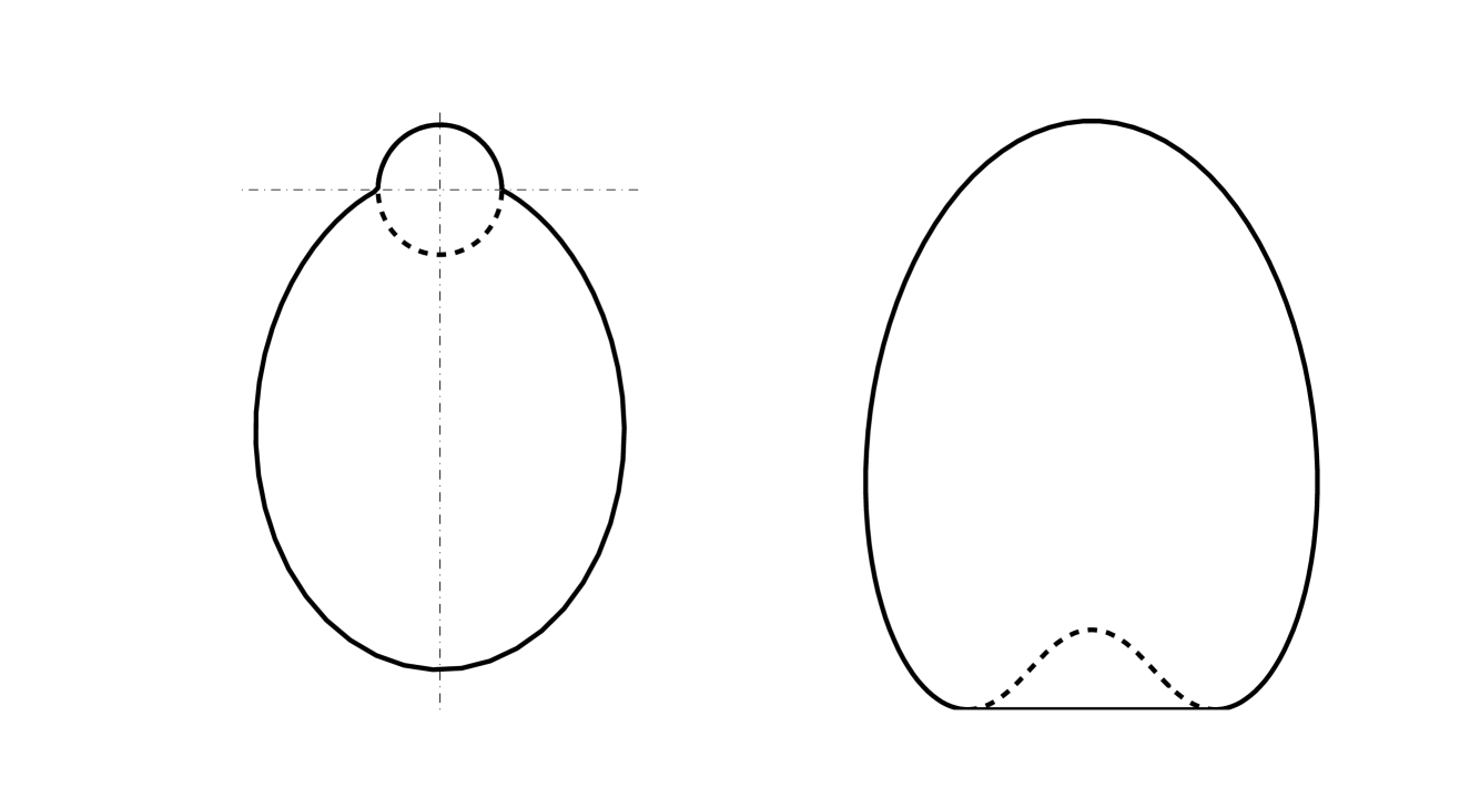
Figure 1. The unit disc, its envelope, and their image

Note the lower semicircle $x^{2}+y^{2}=1$, $y<0$, is mapped via $Z_{0}$ into the interior of $Z_{0}(D)$. Hence, any continuous solution in $D$ extends through the lower semicircle. In fact, the function $\rho$ (defined in (3.6)) in this case is given by $\rho(\theta)=\textrm{e}^{\lvert\sin\theta\rvert}$. The envelope $D_{L}$ of $D$ is the interior of the curve given by $\textrm{e}^{\left(\lvert\sin\theta\rvert-\sin\theta\right)}\,\textrm{e}^{i\theta}$ (see Figure 1.)

2. Let $k\in\mathbb{Z}^{+}$, $\mu\in\mathbb{R}^{+}+i\mathbb{R}$, and

$$L=r^{\lambda-1}\left[\partial_{\theta}-i\mu(1+k\cos k\theta)r\partial_{r}\right]\,.$$

The first integral is $Z_{\mu}=r^{1/\mu}\textrm{e}^{i(\theta+\sin(k\theta))}$ and the characteristic set $\Sigma$ consists of the $2k$ rays given by the roots of the equation $1+k\cos k\theta=0$. Note that $L$ does not satisfy $\mathrm{condition}\,(\mathcal{P})$ at any point of $\Sigma$. The image, via $Z_{\mu}$, of the unit disc $D$ is the unit disc. If follows that if $u\in C^{0}(D)$ solves $Lu=0$, then $u\in C^{\infty}(D\backslash\{0\})$.

3. Let

$$L=r^{\lambda-1}\left[\partial_{\theta}-i\left(2\cos 2\theta-2\sin 4\theta+i\right)r\partial_{r}\right]\,.$$

We have $\mu=i$ and the first integral is

$$Z_{i}=r^{1/i}\exp\left[\sin 2\theta+\frac{1}{2}\cos 4\theta\right]\,\textrm{e}^{i\theta}\,.$$

Figure 2. The annulus $\mathbb{A}(\textrm{e}^{-3/2},\textrm{e}^{3/4})$ and the image of the unit circle (dotted curve)

The characteristic set $\Sigma$ consists of eight rays:

$$\theta=\frac{\pi}{4};\ \frac{3\pi}{4};\ \frac{5\pi}{4};\ \frac{7\pi}{4};\ \frac{\pi}{12};\ \frac{5\pi}{12};\ \frac{13\pi}{12};\ \frac{17\pi}{12}\,.$$

The vector field $L$ does not satisfy $\mathrm{condition}\,(\mathcal{P})$ on any point of $\Sigma$. The function $\lvert Z_{i}\rvert$ reaches a maximum $\textrm{e}^{3/4}$ on the four rays $\displaystyle\theta=\frac{\pi}{12};\ \frac{5\pi}{12};\ \frac{13\pi}{12};\ \frac{17\pi}{12}$; and it reaches a minimum $\textrm{e}^{-3/2}$ on the two rays $\displaystyle\theta=\frac{3\pi}{4};\ \frac{7\pi}{4}$. We have then $Z_{i}(\mathbb{R}^{2}\backslash\{0\})=\mathbb{A}(\textrm{e}^{-3/2},\textrm{e}^{3/4})$. Hence, any $C^{0}$ solution of $Lu=0$ in a region containing an annulus $\mathbb{A}(r_{1},r_{2})$ with $r_{2}>r_{1}\textrm{e}^{2\pi}$ extends to a continuous solution $\widehat{u}$ in $\mathbb{R}^{2}\backslash\{0\}$. Furthermore, $\widehat{u}$ is $C^{\infty}$ everywhere except possibly on the rays where $\lvert Z_{i}\rvert$ reaches its extreme values. In particular, $\widehat{u}$ is $C^{\infty}$ on the rays $\displaystyle\theta=\frac{\pi}{4};\ \frac{5\pi}{4}$ even though $L$ does not satisfy $\mathrm{condition}\,(\mathcal{P})$ along these rays.

5. The equation $Lu=f$ with $f$ homogeneous

In this section, we consider the equation

(5.1) $$Lu=f$$

with $f$ a homogeneous function of degree $\sigma\in\mathbb{C}$. We have following theorem

Theorem 5.1.

Let $l\geq 0$ and $f\in C^{l}(\mathbb{R}^{2}\backslash\{0\})$ be $\sigma$-homogeneous with $\mathrm{Re}(\sigma)>0$. Let $\mu=\mu(L)$ and assume that

(5.2) $$\mu(\lambda-\sigma-1)\notin\mathbb{Z}\,.$$

Then equation $(5.1)$ has a distribution solution $u\in\mathcal{D}^{\prime}(\mathbb{R}^{2})$, with $u$ homogeneous with degree $\sigma+1-\lambda$ and such that $u\in C^{l+1}(\mathbb{R}^{2}\backslash\{0\})$. In particular, if $\mathrm{Re}(\sigma)>\mathrm{Re}(\lambda)-1$, then $u$ is Hölder continuous at 0.

Proof.

Since $f$ is homogeneous, then $f(r,\theta)=r^{\sigma}f_{0}(\theta)$ with $f_{0}\in C^{l}(\mathbb{S}^{1})$. Let

(5.3) $$\psi(\theta)=\int_{0}^{\theta}\frac{q(s)}{p(s)}\,ds$$

so that $\psi(2\pi)=2\pi\mu$. The function

(5.4) $$v(\theta)=\left[K+\int_{0}^{\theta}\frac{f_{0}(s)}{p(s)}\exp\left(-i(\sigma+1-\lambda)\psi(s)\right)\,ds\right]\exp\left(i(\sigma+1-\lambda)\psi(\theta)\right)$$

with $K\in\mathbb{C}$ is the general solution of the following ODE

(5.5) $$p(\theta)v^{\prime}(\theta)-i(\sigma+1-\lambda)q(\theta)v(\theta)=f_{0}(\theta)\,.$$

Since, $\textrm{e}^{2\pi i\mu(\sigma+1-\lambda)}\neq 1$ (by (5.2) and $\psi(2\pi)=2\pi\mu$), then the only periodic solution of (5.5) is obtained when

(5.6) $$K=\frac{1}{1-\textrm{e}^{2\pi i\mu(\sigma+1-\lambda)}}\int_{0}^{2\pi}\frac{f_{0}(s)}{p(s)}\exp\left(-i(\sigma+1-\lambda)\psi(s)\right)\,ds\,.$$

With this value of $K$, let

(5.7) $$u(r,\theta)=r^{\sigma+1-\lambda}v(\theta)\,.$$

Then, $u\in C^{l+1}(\mathbb{R}^{2}\backslash\{0\})$ and it is Hölder continuous at 0 if $\mathrm{Re}(\sigma)>\mathrm{Re}(\lambda)-1$. A simple calculation shows that $u$ solves (5.1) in $\mathbb{R}^{2}\backslash\{0\}$. Now we show that $u$ solves (5.1) in $\mathbb{R}^{2}$ in the sense of distributions. Observe that when $L$ is given by (1.2), then its transpose is

(5.8) $$\begin{array}[]{ll}{}^{t}L&=-(L+\mathrm{div}L)\\ \\ &=-r^{\lambda-1}\left[p(\theta)\partial_{\theta}-iq(\theta)r\partial_{r}-i(\lambda+1)q(\theta)+p^{\prime}(\theta)\right]\,.\end{array}$$

Consider the case $\mathrm{Re}(\sigma)>\mathrm{Re}(\lambda)-2$, so that $u\in L^{1}(\mathbb{R}^{2})$. Then, for $\Phi\in C_{0}^{\infty}(\mathbb{R}^{2})$ a test function, we have

(5.9) $$\begin{array}[]{ll}\langle Lu,\Phi\rangle&=\langle u,\,^{t}L\Phi\rangle\\ &=\displaystyle-\int_{0}^{\infty}\!\!\!\int_{0}^{2\pi}\!\!\!r^{\sigma+1}v\left(p\Phi_{\theta}-irq\Phi_{r}-i(\lambda+1)q\Phi+p^{\prime}\Phi\right)\,d\theta dr\,.\end{array}$$

We use integration by parts together with (5.5) to get

(5.10) $$\begin{array}[]{ll}\displaystyle\int_{0}^{2\pi}\!\!\!p(\theta)v(\theta)\Phi_{\theta}d\theta&=\displaystyle-\int_{0}^{2\pi}\!\!\!\left[p^{\prime}v+i(\sigma+1-\lambda)qv+f_{0}\right]\Phi\,d\theta\\ \\ \displaystyle\int_{0}^{\infty}\!\!\!r^{\sigma+2}\Phi_{r}dr&=\displaystyle-\int_{0}^{\infty}\!\!\!(\sigma+2)r^{\sigma+1}\Phi dr\,.\end{array}$$

After using (5.10) in (5.9), we obtain

(5.11) $$\langle Lu,\Phi\rangle=\int_{0}^{\infty}\!\!\!\int_{0}^{2\pi}\!\!\!r^{\sigma+1}f_{0}(\theta)\Phi(r,\theta)d\theta dr=\langle f,\Phi\rangle$$

The theorem is proved in this case.

Next, suppose that $0<\mathrm{Re}(\sigma)\leq\mathrm{Re}(\lambda)-2$. Let $k=[\mathrm{Re}(\lambda-\sigma)]$, where $[x]$ denotes the greatest integer $\leq x$. Define $u\in\mathcal{D}^{\prime}(\mathbb{R}^{2})$ by

(5.12) $$\langle u,\Phi\rangle=C_{0}\int_{0}^{\infty}\!\!\!\int_{0}^{2\pi}\!\!\!r^{k-(\lambda-\sigma)}v(\theta)\displaystyle\frac{\partial^{\,k-2}\Phi}{\partial r^{k-2}}\,d\theta dr\,,\quad\Phi\in C^{\infty}_{c}(\mathbb{R}^{2})$$

where

$$C_{0}=\frac{\Gamma(\lambda-\sigma-k)}{\Gamma(\lambda-\sigma-2)}$$

and $\Gamma$ is the gamma function. Since we are using derivatives with the polar coordinate, we need to verify that (5.12) indeed defines a distribution. We have

$$\frac{\partial^{\,n}}{\partial r^{n}}=\sum_{j=0}^{n}\Big{(}\,^{n}_{j}\Big{)}\cos^{n-j}\theta\sin^{j}\theta\displaystyle\frac{\partial^{\,n}}{\partial x^{n-j}\partial y^{j}}$$

(this formula can be established by induction), and for a compact set $K\subset\mathbb{R}^{2}$ with $\hbox{\rm supp\,}\Phi\subset K$, we have

$$\lvert\langle u,\Phi\rangle\rvert\,\leq\,C(K)\,\sum_{j=0}^{k-2}\sup_{K}\left|\displaystyle\frac{\partial^{k-2}\Phi}{\partial x^{k-2-j}\partial y^{j}}\right|$$

where $C(K)$ is a constant depending only on $K$, $v$, $\sigma$, and $\lambda$. To verify the homogeneity of $u$, define the distribution $u_{s}\in\mathcal{D}^{\prime}(\mathbb{R}^{2})$ (with $s>0$) by $\langle u_{s},\Phi\rangle=s^{-2}\langle u,\Phi(x/s,y/s)\rangle$. We have

$$\frac{\partial^{\,k-2}}{\partial r^{k-2}}\left(\Phi(\frac{r}{s},\theta)\right)=\frac{1}{s^{k-2}}\displaystyle\frac{\partial^{k-2}\Phi}{\partial r^{k-2}}\left(\frac{r}{s},\theta\right)$$

and the change of variable $\rho=r/s$ in the integral defining $u_{s}$ gives

$$\begin{array}[]{ll}\langle u_{s},\Phi\rangle&=\displaystyle s^{-2}C_{0}\int_{0}^{\infty}\!\!\!\int_{0}^{2\pi}\!\!\!s^{\sigma-\lambda+3}\rho^{k-(\lambda-\sigma)}v(\theta)\displaystyle\frac{\partial^{\,k-2}\Phi}{\partial\rho^{k-2}}(\rho,\theta)\,d\theta d\rho\\ &=s^{\sigma-\lambda+1}\langle u,\Phi\rangle\,.\end{array}$$

This shows the homogeneity of $u$. Now we verify that $u$ solves (5.1). The function ${}^{t}L\Phi$ has compact support and vanishes to order $\mathrm{Re}(\lambda)-1$ at the origin ($r=0$). We can use integration by parts to obtain

$$\begin{array}[]{ll}\langle Lu,\Phi\rangle&=\langle u,\,^{t}L\Phi\rangle=\displaystyle C_{0}\int_{0}^{\infty}\!\!\!\int_{0}^{2\pi}\!\!\!r^{k-(\lambda-\sigma)}v\displaystyle\frac{\partial^{\,k-2}{\,{}^{t}L\Phi}}{\partial r^{k-2}}\,d\theta dr\\ &=\displaystyle C_{1}\int_{0}^{\infty}\!\!\!\int_{0}^{2\pi}\!\!\!r^{k-(\lambda-\sigma)-1}v\displaystyle\frac{\partial^{\,k-3}{\,{}^{t}L\Phi}}{\partial r^{k-3}}\,d\theta dr\end{array}$$

with

$$C_{1}=(\lambda-\sigma-k)C_{0}=\frac{\Gamma(\lambda-\sigma-k+1)}{\Gamma(\lambda-\sigma-2)}\,.$$

In general after $j$ integrations by parts (with $j\leq k-2$) we get

$$\langle Lu,\Phi\rangle=\frac{\Gamma(\lambda-\sigma-k+j)}{\Gamma(\lambda-\sigma-2)}\,\int_{0}^{\infty}\!\!\!\int_{0}^{2\pi}\!\!\!r^{k-(\lambda-\sigma)-j}v\displaystyle\frac{\partial^{\,k-2-j}{\ {}^{t}L\Phi}}{\partial r^{k-2-j}}\,d\theta dr\,.$$

In particular, for $j=k-2$, we obtain

$$\langle Lu,\Phi\rangle=\int_{0}^{\infty}\!\!\!\int_{0}^{2\pi}\!\!\!r^{\sigma-\lambda+2}v(\theta)\,^{t}L\Phi\,d\theta dr\,.$$

Finally, a calculation similar to that carried out in the case $\mathrm{Re}(\sigma)>\mathrm{Re}(\lambda)-2$, gives

$$\langle Lu,\Phi\rangle=\int\!\!\int_{\mathbb{R}^{2}}f(x,y)\Phi(x,y)dxdy\,.$$

∎

When (5.2) does not hold, then equation (5.1) can still be solved, provided that $f$ satisfies a compatibility condition.

Theorem 5.2.

Suppose that $\mu(\sigma+1-\lambda)\in\mathbb{Z}$. If $f(r,\theta)=r^{\sigma}f_{0}(\theta)$ satisfies

(5.13) $$\int_{0}^{2\pi}\!\!\!\frac{f_{0}(s)}{p(s)}\exp\left[-i\mu(\sigma+1-\lambda)\psi(s)\right]\,ds=0\,,$$

where $\psi$ is given by $(5.3)$, then equation $(5.1)$ has a homogeneous distribution solution as that given in Theorem $5.1$.

The proof is identical to that of Theorem 5.1. This time we define $v$ by (5.4) with constant $K=0$.

Now, for a class of vector fields, we consider equation (5.1) when $f=\delta$, the Dirac distribution. More precisely, we have the following result.

Theorem 5.3.

Suppose that $\mathrm{div}L=0$; the homogeneity degree of $L$ is $\lambda=N\in\mathbb{Z}^{+}$; and that $\mu\neq 0$. Then, the distribution $u\in\mathcal{D}^{\prime}(\mathbb{R}^{2})$ given by

(5.14) $$\langle u,\Phi\rangle=\frac{1}{2\pi i\mu(N-1)!}\int_{0}^{\infty}\!\!\!\int_{0}^{2\pi}\!\!\!\frac{\ln r}{p(\theta)}\displaystyle\frac{\partial\,^{N}\Phi}{\partial r^{N}}\,d\theta dr\,,\quad\Phi\in C^{\infty}_{c}(\mathbb{R}^{2})$$

satisfies the equation $Lu=\delta$.

Proof.

For a test function $\Phi$, we have $r^{N}\Phi=O(r^{N})$ as $r\,\longrightarrow\,0$, and integration by parts gives

$$\int_{0}^{\infty}\!\!\!\ln r\,\displaystyle\frac{\partial\,^{N}(r^{N}\Phi)}{\partial r^{N}}\,dr=-\int_{0}^{\infty}\!\!\!r^{-1}\,\displaystyle\frac{\partial\,^{N-1}(r^{N}\Phi)}{\partial r^{N-1}}\,dr\,.$$

By repeated integration by parts, $N$ times, we get

(5.15) $$\int_{0}^{\infty}\!\!\!\ln r\,\displaystyle\frac{\partial\,^{N}(r^{N}\Phi)}{\partial r^{N}}\,dr=-(N-1)!\int_{0}^{\infty}\!\!\!\Phi(r,\theta)\,dr\,.$$

Since $\mathrm{div}L=0$, then $\langle Lu,\Phi\rangle=-\langle u,L\Phi\rangle$ and

(5.16) $$\langle Lu,\Phi\rangle=\displaystyle\frac{-1}{2\pi i\mu(N-1)!}\!\int_{0}^{\infty}\!\!\!\!\int_{0}^{2\pi}\!\!\!\ln r\displaystyle\frac{\partial\,^{N}(r^{N-1}\Phi_{\theta})}{\partial r^{N}}-i\frac{q(\theta)}{p(\theta)}\ln r\displaystyle\frac{\partial\,^{N}(r^{N}\Phi_{r})}{\partial r^{N}}\,d\theta dr$$

We have

(5.17) $$\int_{0}^{2\pi}\!\!\displaystyle\frac{\partial\,^{N}(r^{N-1}\Phi_{\theta})}{\partial r^{N}}\,d\theta=\int_{0}^{2\pi}\!\!\left(\displaystyle\frac{\partial\,^{N}(r^{N-1}\Phi)}{\partial r^{N}}\right)_{\theta}\,d\theta\,=0\,.$$

Expressions (5.15) and (5.17) give

(5.18) $$\int_{0}^{\infty}\!\!\!\ln r\displaystyle\frac{\partial\,^{N}(r^{N}\Phi_{r})}{\partial r^{N}}\,dr=-(N-1)!\int_{0}^{\infty}\!\!\!\Phi_{r}(r,\theta)dr=(N-1)!\Phi(0)\,.$$

After using (5.17) and (5.18), (5.16) becomes

$$\langle Lu,\Phi\rangle=\frac{1}{2\pi\mu}\int_{0}^{2\pi}\frac{q(\theta)}{p(\theta)}\Phi(0)d\theta=\Phi(0)\,.$$

∎

6. Equation $Lu=f$ with $f$ real analytic

In this section, we consider the equation

(6.1) $$Lu=f$$

with $f$ real analytic in a neighborhood of $0\in\mathbb{R}^{2}$. We show that this equation has a distribution solution which is smooth outside 0 when the numbers $\mu$ and $\lambda$ attached to $L$ satisfy a certain diophantine condition.

Let $\mu,\,\lambda\,\in\mathbb{C}$ be the numbers associated with $L$, with $\mathrm{Re}(\mu)\geq 0$ and $\mathrm{Re}(\lambda)>1$. We say that the pair $(\mu,\lambda)$ is resonant if $\mu\lambda\in\mu\mathbb{Z}^{+}+\mathbb{Z}$. That is, if there exist $l,k\in\mathbb{Z}$, with $l\geq 1$, such that $\mu\lambda=\mu l+k$. We call such a number $l$ a resonant integer for $(\mu,\lambda)$. Denote by $\mathbb{J}(\mu,\lambda)$ the set of resonant integers for $(\mu,\lambda)$. Note that when $f$ is a homogeneous function of degree $(j-1)$ and $j$ is a resonant integer for $(\mu,\lambda)$, then the equation $Lu=f$ does not have a homogeneous solution unless $f$ satisfies a compatibility condition.

Lemma 6.1.

Suppose that $(\mu,\lambda)$ is resonant. Then

• If $(\mu,\lambda)\not\in\mathbb{Q}^{+}\times\mathbb{Q}^{+}$, then $(\mu,\lambda)$ has a unique resonant integer.

• If $\mu\in\mathbb{Q}^{+}$ or if $\lambda\in\mathbb{Q}^{+}$, then $(\mu,\lambda)$ has infinitely many resonant integers.

Proof.

First note that since $(\mu,\lambda)$ is resonant, then if one of the numbers $\mu$ or $\lambda$ is in $\mathbb{Q}^{+}$, then so is the other. Let $(j_{0},k_{0})\in\mathbb{Z}^{+}\times\mathbb{Z}$ be such that $\mu\lambda=\mu j_{0}+k_{0}$. If $(j_{1},k_{1})\in\mathbb{Z}^{+}\times\mathbb{Z}$ is any other pair satisfying $\mu\lambda=\mu j_{1}+k_{1}$, then $\mu(j_{1}-j_{0})=k_{0}-k_{1}$ and $\mu\in\mathbb{Q}$. Conversely, if $\mu=m/n$ with $m,n\in\mathbb{Z}^{+}$ and $\gcd(m,n)=1$. $j=j_{0}+ln$, $k=k_{0}-lm$ satisfies $\mu\lambda=\mu j+k$ for any $l\in\mathbb{Z}$. ∎

Lemma 6.2.

Suppose that $\mathrm{div}L=0$. The associated pair $(\mu,\lambda)$ is resonant if and only if either $\mu=0$ or if $\lambda\in\mathbb{Q}^{+}$. In this case the pair has infinitely many resonant integers. In particular, if in addition $L$ is real analytic at 0 with homogeneous degree $\lambda=N\in\mathbb{Z}^{+}$, then $(\mu,N)$ is resonant with infinitely many resonant integers.

Proof.

Since $\mathrm{div}L=0$, then $\mu=p/(\lambda+1)$ for some $p\in\mathbb{Z}$, $p\geq 0$ (Remark 2.1). If $p=0$, the pair $(0,\lambda)$ is trivially resonant. Suppose that $p\geq 1$. If $(\mu,\lambda)$ is resonant, then there exists $(l_{0},k_{0})\in\mathbb{Z}^{+}\times\mathbb{Z}$ such that $p\lambda/(\lambda+1)=pl_{0}/(\lambda+1)\,+k_{0}$. Therefore, $\lambda(p-k_{0})=pl_{0}+k_{0}$ and $\lambda\in\mathbb{Q}^{+}$. Conversely, if $\lambda=m/n$ with $m,n\,\in\mathbb{Z}^{+}$ and $\gcd(m.n)=1$, then $\mu=p/(\lambda+1)=pn/(m+n)$. It can be verified that for every $s\in\mathbb{Z}^{+}$, $j=s(m+n)-1$ is $(\mu,\lambda)$-resonant with a corresponding $k=p(1-sn)$. ∎

Now we introduce a condition $(\mathcal{DC})$ for nonresonant pairs $(\mu,\lambda)$.

• : There exists $C>0$ such that for every $j\in\mathbb{Z}^{+}$

  $$\left|1-\textrm{e}^{2\pi i\mu(j-\lambda)}\right|\geq C^{j}$$

Proposition 6.1.

Suppose that $\mu\in\mathbb{C}$, $\mu\neq 0$, $\mathrm{Re}(\mu)\geq 0$ and $\lambda\in\mathbb{C}$, are such that $(\mu,\lambda)$ is nonresonant. Then,

• If $\mu\notin\mathbb{R}$, then $(\mu,\lambda)$ satisfies condition $(\mathcal{DC})$.

• If $\mu\in\mathbb{R}^{+}$ and $\lambda\notin\mathbb{R}$, then $(\mu,\lambda)$ satisfies condition $(\mathcal{DC})$.

• If $\mu,\,\lambda\,\in\mathbb{R}^{+}$, then condition$(\mathcal{DC})$ holds if and only if the following condition holds

  • : There exists $C>0$ such that for every $j\in\mathbb{Z}^{+}$ and $k\in\mathbb{Z}$

    $$\left|\mu(j-\lambda)-k\right|\geq C^{j}$$

Proof.

Let $\mu=\mu_{1}+i\mu_{2}$, $\lambda=\lambda_{1}+i\lambda_{2}$ with $\mu_{1},\mu_{2},\lambda_{1},\lambda_{2}\in\mathbb{R}$ and $\mu_{1},\lambda_{1}\geq 0$. Then for $j\in\mathbb{Z}^{+}$ we have

(6.2) $$\textrm{e}^{2\pi i\mu(j-\lambda)}=\textrm{e}^{2\pi(\mu_{1}\lambda_{2}+\mu_{2}\lambda_{1}-\mu_{2}j)}\,\textrm{e}^{2\pi i(\mu_{1}j-\mu_{1}\lambda_{1}+\mu_{2}\lambda_{2})}$$

and since $(\mu,\lambda)$ is nonresonant, then for every $j\in\mathbb{Z}^{+}$, $k\in\mathbb{Z}$,

(6.3) $$(\mu_{1}\lambda_{1}-\mu_{2}\lambda_{2}-j\mu_{1}-k)+i(\mu_{1}\lambda_{2}+\mu_{2}\lambda_{1}-j\mu_{2})\,\neq 0$$

Suppose that $\mu_{2}\neq 0$. If for every $j\in\mathbb{Z}^{+}$ $\mu_{1}\lambda_{2}+\mu_{2}\lambda_{1}-j\mu_{2}\neq 0$, then

(6.4) $$\min_{j\in\mathbb{Z}^{+}}\left|1-\textrm{e}^{2\pi(\mu_{1}\lambda_{2}+\mu_{2}\lambda_{1}-j\mu_{2})}\right|\,>0\,.$$

Consequently the pair $(\mu,\lambda)$ satisfies $(\mathcal{DC})$. If there exists $j_{0}\in\mathbb{Z}^{+}$ such that $\mu_{1}\lambda_{2}+\mu_{2}\lambda_{1}-j_{0}\mu_{2}=0$, then $\left|\textrm{e}^{2\pi i\mu(j_{0}-\lambda)}\right|=1$. It follows from (6.3) that, for every $k\in\mathbb{Z}$, we necessarily have $\mu_{1}\lambda_{1}-\mu_{2}\lambda_{2}-j_{0}\mu_{1}-k\neq 0$. Hence,

(6.5) $$\left|\textrm{e}^{2\pi i\mu(j_{0}-\lambda)}-1\right|>0$$

and we also have

(6.6) $$\min_{j\in\mathbb{Z}^{+},\,j\neq j_{0}}\left|1-\textrm{e}^{2\pi(\mu_{1}\lambda_{2}+\mu_{2}\lambda_{1}-j\mu_{2})}\right|\,>0\,.$$

Inequalities (6.5), (6.6) imply that the pair $(\mu,\lambda)$ satisfies $(\mathcal{DC})$, which proves part (a).

Next, suppose that $\mu=\mu_{1}\in\mathbb{R}^{+}$ and $\lambda_{2}\neq 0$. Then for every $j\in\mathbb{Z}$, $\left|\textrm{e}^{2\pi i\mu_{1}(j-\lambda)}\right|=\textrm{e}^{2\pi\mu_{1}\lambda_{2}}\neq 1$ and part (b) follows.

To prove part (c), suppose that $\mu=\mu_{1}>0$ and $\lambda=\lambda_{1}>0$. We need to show that conditions $(\mathcal{DC})$ and $(\mathcal{DC}^{\prime})$ are equivalent. If $(\mathcal{DC}^{\prime})$ does not hold, then for every $l\in\mathbb{Z}^{+}$, there exists $j_{l}\in\mathbb{Z}^{+}$ and $k_{l}\in\mathbb{Z}$ such that

(6.7) $$\left|\mu(j_{l}-\lambda)-k_{l}\right|\,<\,l^{-j_{l}}\,.$$

We have then

(6.8) $$\begin{array}[]{ll}\displaystyle\left|\textrm{e}^{2\pi i\mu(j_{l}-\lambda)}-1\right|^{2}&=\displaystyle\left|\textrm{e}^{2\pi i\left[\mu(j_{l}-\lambda)-k_{l}\right]}-1\right|^{2}\\ \\ &=\displaystyle 2\left(1-\cos\left[2\pi(\mu(j_{l}-\lambda)-k_{l})\right]\right)\\ \\ &=\displaystyle 4\pi\left[\mu(j_{l}-\lambda)-k_{l}\right]\,\sin\theta_{l}\end{array}$$

for some $\theta_{l}$. This, together with (6.7), give

(6.9) $$\left|\textrm{e}^{2\pi i\mu(j_{l}-\lambda)}-1\right|^{2}\,<\,4\pi l^{-j_{l}}$$

which means that $(\mathcal{DC})$ does not hold.

Conversely, suppose that $(\mathcal{DC})$ does not hold. Then for every $l\in\mathbb{Z}^{+}$, there exists $j_{l}\in\mathbb{Z}^{+}$ such that

(6.10) $$\left|\textrm{e}^{2\pi i\mu(j_{l}-\lambda)}-1\right|\,<\,l^{-j_{l}}\,.$$

Let $k_{l}=[\mu(j_{l}-\lambda)]$. Since $0\leq\mu(j_{l}-\lambda)-k_{l}<1$, it follows from (6.10) that $\displaystyle\lim_{l\to\infty}(\mu(j_{l}-\lambda)-k_{l})=0$. Consequently, after using $\lvert\textrm{e}^{i\alpha}-1\rvert^{2}=2(1-\cos\alpha)>\alpha^{2}$ (for $\alpha$ small), we obtain

$$l^{-2j_{l}}\,>\,\displaystyle\left|\textrm{e}^{2\pi i(\mu(j_{l}-\lambda)-k_{l})}-1\right|^{2}\,>\,\displaystyle 4\pi\left|\mu(j_{l}-\lambda)-k_{l}\right|^{2}$$

and therefore $(\mathcal{DC}^{\prime})$ does not hold. ∎

Theorem 6.1.

Let $L$ be a $\lambda$-homogeneous vector field with $\mu\neq 0$ and such that the pair $(\mu,\lambda)$ is nonresonant and satisfies condition $(\mathcal{DC})$. Then for every function $f(x,y)$ that is real analytic at $0\in\mathbb{R}^{2}$, there exist $\epsilon>0$ and a bounded function $w\in C^{\infty}(D(0,\epsilon)\backslash\{0\})$ such that $u=w/r^{\lambda-1}$ is a distribution solution of $(6.1)$ in the disc $D(0,\epsilon)$.

Proof.

We expand the real analytic function $f$ as

(6.11) $$f(x,y)=\sum_{j=0}^{\infty}P_{j}(x,y)\,\ \ \mathrm{with}\ \ P_{j}(x,y)=\sum_{k+l=j}\frac{1}{k!l!}\displaystyle\frac{\partial\,^{j}f}{\partial x^{k}\partial y^{l}}(0)\,x^{k}y^{l}\,.$$

Let

(6.12) $$P_{j}(x,y)=r^{j}f_{j}(\theta)\ \ \mathrm{with}\ \ f_{j}(\theta)=\sum_{k+l=j}\frac{1}{k!l!}\displaystyle\frac{\partial\,^{j}f}{\partial x^{k}\partial y^{l}}(0)\,\cos^{k}\theta\sin^{l}\theta$$

Let $R>0$ be such that the function $f(x,y)$ has a holomorphic extension $\widehat{f}(\widehat{x},\widehat{y})$ in an open neighborhood of the bidisc $D(0,R)^{2}\subset\mathbb{C}^{2}$. Let $\displaystyle M_{0}=\max_{\lvert\widehat{x}\rvert,\,\lvert\widehat{y}\rvert\,\leq R}\left|\widehat{f}(\widehat{x},\widehat{y})\right|$. It follows from the Cauchy integral formula that

$$\left|\displaystyle\frac{\partial\,^{j}f}{\partial x^{k}\partial y^{l}}(0)\right|\,\leq\,k!l!\,\frac{M_{0}}{R^{j}}\,.$$

Hence, we get the estimate

(6.13) $$\left|f_{j}(\theta)\right|\,\leq\,(j+1)\frac{M_{0}}{R^{j}}\qquad\forall\theta\,.$$

Let

(6.14) $$\psi(\theta)=\int_{0}^{\theta}\frac{q(s)}{p(s)}\,ds=\psi_{1}(\theta)+i\psi_{2}(\theta)$$

so that $\psi(2\pi)=2\pi\mu$. Define $v_{j}(\theta)\in C^{\infty}(\mathbb{R}^{2}\backslash\{0\})$ by

(6.15) $$v_{j}(\theta)=\left[K_{j}+\int_{0}^{\theta}\!\!\frac{f_{j}(s)}{p(s)}\,\textrm{e}^{-i(j+1-\lambda)\psi(s)}ds\right]\textrm{e}^{i(j+1-\lambda)\psi(\theta)}$$

with

(6.16) $$K_{j}=\frac{1}{1-\textrm{e}^{2\pi i\mu(j+1-\lambda)}}\int_{0}^{2\pi}\!\!\frac{f_{j}(s)}{p(s)}\,\textrm{e}^{-i(j+1-\lambda)\psi(s)}ds\,.$$

Note that the denominator in $K_{j}$ is not zero since the pair $(\mu,\lambda)$ is nonresonant. The function $v_{j}$ is a periodic solution of the differential equation

(6.17) $$p(\theta)v^{\prime}(\theta)-i(j+1-\lambda)q(\theta)v(\theta)=f_{j}(\theta)\,.$$

Therefore $r^{j+1-\lambda}v_{j}(\theta)$ is the homogeneous distribution solution of $Lu=P_{j}$ given in Theorem 5.1. Consider the series

(6.18) $$w(r,\theta)=\sum_{j=0}^{\infty}v_{j}(\theta)r^{j}\,.$$

We prove that $w$ is a $C^{\infty}$ function of $(r,\theta)$ for small $r$. Let $\lambda_{1}$ and $\lambda_{2}$ be the real and imaginary parts of $\lambda$. Then

$$\left|\textrm{e}^{-i(j+1-\lambda)\psi(s)}\right|=\textrm{e}^{-\lambda_{1}\psi_{2}(s)-\lambda_{2}\psi_{1}(s)}\left(\textrm{e}^{\psi_{2}(s)}\right)^{j+1}\,.$$

Set

$$M_{1}=\max_{0\leq s\leq 2\pi}\textrm{e}^{-\lambda_{1}\psi_{2}(s)-\lambda_{2}\psi_{1}(s)}\,;\ \ \displaystyle M_{2}=\max_{0\leq s\leq 2\pi}\textrm{e}^{\psi_{2}(s)}\,;\ \ \mathrm{and}\ \ \displaystyle p_{0}=\min_{0\leq s\leq 2\pi}\lvert p(s)\rvert\,.$$

Then, it follows from (6.13), that for $0\leq\theta\leq 2\pi$, we have

(6.19) $$\left|\int_{0}^{\theta}\!\!\frac{f_{j}(s)}{p(s)}\textrm{e}^{-i(j+1-\lambda)\psi(s)}\,ds\right|\,\leq\,\frac{2\pi M_{1}M_{0}(j+1)M_{2}^{j+1}}{p_{0}R^{j}}\,\leq\,C_{0}^{j}$$

for some constant $C_{0}$ depending only on $f$, $\lambda$, $p$ and $q$. Since $(\mu,\lambda)$ satisfies the diophantine condition $(\mathcal{DC})$, it follows from (6.16) and (6.19) that

(6.20) $$\lvert K_{j}\rvert\,\leq\,C_{1}^{j}\,\ \ \mathrm{with}\ \ C_{1}=\frac{C_{0}}{C}\,.$$

This inequality, together with (6.15) and (6.19), imply that

(6.21) $$\left|v_{j}(\theta)\right|\,\leq\,(C_{1}^{j}+C_{0}^{j})M_{1}M_{2}^{j+1}\,\leq\,C_{2}^{j}$$

with a constant $C_{2}>0$ depending only on $f$, $\lambda$, $p$ and $q$. This proves at once that the series defining $w$ given by (6.18) converges uniformly for $\theta\in[0,\ 2\pi]$ and $r\in[0,\ R_{0}]$ for any positive number $R_{0}<1/C_{2}$. Consequently, $w(r,\theta)$ is continuous, $2\pi$-periodic in $\theta$ and real analytic in $r$. The uniform convergence of the series of derivatives can be proved by a similar argument. For instance, since

$$v^{\prime}_{j}(\theta)=i(j+1-\lambda)\frac{q(\theta)}{p(\theta)}v_{j}(\theta)+\frac{f_{j}(\theta)}{p(\theta)}$$

then similar estimates show that $\sum v^{\prime}_{j}(\theta)r^{j}$ is again uniformly convergent and so $w\in C^{1}$ in the $(r,\theta)$ variables. This argument can be repeated for the successive derivatives leading to $w\in C^{\infty}([0,\ R_{0}]\times\mathbb{S}^{1})$.

Let $u=w/r^{\lambda-1}$. We can write

(6.22) $$u(r,\theta)=\sum_{j=0}^{[\mathrm{Re}(\lambda)]}\!v_{j}(\theta)r^{j+1-\lambda}+\sum_{j=[\mathrm{Re}(\lambda)]+1}^{\infty}\!\!v_{j}(\theta)r^{j+1-\lambda}\,.$$

The finite sum in (6.22) is a distribution solution of the equation
$Lg=\sum_{j=0}^{[\mathrm{Re}(\lambda)]}P_{j}\,$ and the infinite sum, which is a function of at least class $C^{1}$ at $0\in\mathbb{R}^{2}$, solves the equation $Lg=f-\sum_{j=0}^{[\mathrm{Re}(\lambda)]}P_{j}$. This completes the proof of the theorem. ∎

Remark 6.1.

Diophantine conditions such as the one used here appear in connection with the hypoellipticity and solvability. For instance in [2], [3], the analytic solvability in a neighborhood of a degeneracy curve of a vector field is controlled by a Diophantine condition.

Theorem 6.2.

Suppose that $(\mu,\lambda)$ is nonresonant, satisfies $(\mathcal{DC})$, and that $\mathrm{Re}(\mu)>0$. Let $f$ be a real analytic function in a neighborhood of $0\in\mathbb{R}^{2}$. If $u$ is a distribution solution of $(6.1)$ such that $u$ is continuous outside 0, then there exists $\epsilon>0$ such that $u\in C^{\infty}(D(0,\epsilon)\backslash\{0\})$.

Proof.

By Theorem 6.1, there exists a distribution solution $u_{0}$ of (6.1) with $u_{0}\in C^{\infty}(D(0,R)\backslash\{0\})$. If $u_{1}$ is any other solution, continuous outside 0, then $u_{0}-u_{1}$ satisfies $L(u_{0}-u_{1})=0$ and is continuous outside 0. Since, $\mathrm{Re}(\mu)>0$, then it follows from Theorem 3.3, that there exists $\epsilon>0$ such that $u_{0}-u_{1}\in C^{\infty}(D(0,\epsilon)\backslash\{0\})$. ∎

Remark 6.2.

If $L$ is real analytic in $\mathbb{R}^{2}\backslash\{0\}$, then the distribution solution constructed in Theorem 6.1 is real analytic in a punctured neighborhood of 0 and so is every solution if $\mathrm{Re}(\mu)>0$.

Now we consider the case when $(\mu,\lambda)$ is resonant. As was observed in section 5, the equation (6.1) with a homogeneous right hand side does not always have a homogeneous solution unless a compatibility condition is satisfied. A real analytic function $f(x,y)$ is $(\mu,\lambda)$-compatible if, its series expansion (6.11) satisfies

(6.23) $$\int_{0}^{2\pi}\!\!\frac{f_{j}(\theta)}{p(\theta)}\textrm{e}^{-i(j+1-\lambda)\psi(\theta)}\,d\theta=0\,,\quad\forall j\in\mathbb{J}(\mu,\lambda)$$

where $f_{j}$ is given by (6.12). Note that when $\mu\notin\mathbb{Q}$, then there is only one resonant integer and (6.23) reduces to a single condition, while if $\mu\in\mathbb{Q}$, then there are infinitely many conditions (see Lemma 6.1). In particular, if, in addition, $L$ is real analytic at $0\in\mathbb{R}^{2}$ and $\mathrm{div}L=0$, then there are infinitely many compatibility conditions (see Lemma 6.2).

Theorem 6.3.

Suppose that $(\mu,\lambda)$ is resonant and satisfies $(\mathcal{DC})$. Then for every $(\mu,\lambda)$-compatible, real analytic function $f$, equation $(6.1)$ has a distribution solution as in Theorem $6.1$

Remark 6.3.

Among the results contained in the recent papers [13], [14] are the solvability and hypoellipticity of vector fields

$$\left(a_{11}x+a_{12}y\right)\partial_{x}+\left(a_{21}x+a_{22}y\right)\partial_{y}$$

with $a_{ij}\in\mathbb{C}$. In particular, such vector fields are not hypoelliptic at 0. This lack of hypoellipticity is generalized in [8] in the real analytic category to vector fields with an isolated singularities.

7. Solvability when $L$ satisfies condition $(\mathcal{P})$

In this section we consider the equation $Lu=f$ with $f$ a $C^{\infty}$ function in a neighborhood of 0 under the assumption that $L$ satisfies $\mathrm{condition}\,(\mathcal{P})$ in $\mathbb{R}^{2}\backslash\{0\}$. We have the following theorem.

Theorem 7.1.

Suppose that the homogeneous vector field $L$ satisfies condition $(\mathcal{P})$ in $\mathbb{R}^{2}\backslash\{0\}$ and $(\mu,\lambda)$ is nonresonant. Then, for every $f\in C^{\infty}(\mathbb{R}^{2})$ there exist $\epsilon>0$ and a continuous function $w(r,\theta)$ in the cylinder $[0,\ \epsilon)\times\mathbb{S}^{1}$ such that $w(0,\theta)=0$ and $w\in C^{\infty}((0,\ \epsilon)\times\mathbb{S}^{1})$ and such that the function $u(x,y)$ defined in polar coordinates by $u=w/r^{\lambda-1}$ is a distribution solution of

(7.1) $$Lu=f\quad\mathrm{in}\quad D(0,\epsilon)\subset\mathbb{R}^{2}\,.$$

Proof.

Let $\sum_{j=0}^{\infty}P_{j}(x,y)$ be the Taylor series of $f$ at $0\in\mathbb{R}^{2}$, where $P_{j}=r^{j}f_{j}(\theta)$ is the homogeneous polynomial given by (6.12). Since the pair $(\mu,\lambda)$ is nonresonant, then for every $j\geq 0$, we can find $v_{j}\in C^{\infty}(\mathbb{S}^{1})$ such that $r^{j}v_{j}(\theta)/r^{\lambda-1}$ is a distribution solution of the equation $Lu=P_{j}$. By using Borel’s Extension Theorem, we can find a function $v(r,\theta)\in C^{\infty}([0,\ \epsilon)\times\mathbb{S}^{1})$, for some $\epsilon>0$, such that

(7.2) $$\frac{\partial\,^{j}v}{\partial r^{j}}(0,\theta)=j!v_{j}(\theta)\,,\quad\forall j\geq 0\,.$$

Then the $r$-Taylor series of the function

(7.3) $$g(r,\theta)=f(r,\theta)-L\left(\frac{v(r,\theta)}{r^{\lambda-1}}\right)$$

is identically zero. That is $\displaystyle\displaystyle\frac{\partial\,^{j}g}{\partial r^{j}}(0,\theta)=0$ for every $j\geq 0$. When considered as a function of $(x,y)$ in a neighborhood of $0\in\mathbb{R}^{2}$, the function $g$ vanishes to infinite order at $0$. Since $L$ satisfies $\mathrm{condition}\,(\mathcal{P})$ in $\mathbb{R}^{2}\backslash\{0\}$, then the vector field

(7.4) $$L_{0}=\partial_{\theta}-i\frac{q(\theta)}{p(\theta)}r\partial_{r}=\frac{L}{p(\theta)r^{\lambda-1}}$$

satisfies $\mathrm{condition}\,(\mathcal{P})$ in $\mathbb{R}\times\mathbb{S}^{1}$. Let

(7.5) $$\Sigma_{0}=\{\theta\in\mathbb{S}^{1}:\ \mathrm{Re}(q(\theta)\overline{p(\theta)})=0\}\,.$$

Since $\Sigma_{0}\subset\mathbb{S}^{1}$ is compact and $L_{0}$ satisfies $\mathrm{condition}\,(\mathcal{P})$, then we can find $\epsilon>0$ and $\theta_{1}\,,\cdots,\theta_{N}\in\mathbb{S}^{1}$ such that

(7.6) $$\begin{array}[]{c}\displaystyle\Sigma_{0}\subset\bigcup_{k=1}^{N}(\theta_{k}-\epsilon,\ \theta_{k}+\epsilon)\,,\\ \displaystyle(\theta_{k}-2\epsilon,\ \theta_{k}+2\epsilon)\cap(\theta_{l}-2\epsilon,\ \theta_{l}+2\epsilon)=\emptyset\ \mathrm{for}\ k\neq l\,.\end{array}$$

Moreover, for each $k=1,\cdots,N$ there exists $w_{k}\in C^{\infty}\left((-\epsilon,\ \epsilon)\times(\theta_{k}-2\epsilon,\ \theta_{k}+2\epsilon)\right)$ such that

(7.7) $$L_{0}w_{k}=\frac{g(r,\theta)}{p(\theta)r^{\lambda-1}}\,.$$

We can furthermore assume that $w_{k}(0,\theta)=0$. Let $w_{0}\in C^{\infty}\left((-\epsilon,\ \epsilon)\times\mathbb{S}^{1}\right)$ be such that

(7.8) $$w_{0}(r,\theta)=w_{k}(r,\theta)\ \ \mathrm{in}\ (-\epsilon,\ \epsilon)\times(\theta_{k}-\epsilon,\ \theta_{k}+\epsilon)\,,\ \ \mathrm{for}\ k=1,\cdots,N$$

Hence, $L_{0}w_{0}\in C^{\infty}\left((-\epsilon,\ \epsilon)\times\mathbb{S}^{1}\right)$ and

(7.9) $$L_{0}w_{0}(r,\theta)=\frac{g(r,\theta)}{p(\theta)r^{\lambda-1}}\ \ \mathrm{in}\ \ \bigcup_{k=1}^{N}(-\epsilon,\ \epsilon)\times(\theta_{k}-\epsilon,\ \theta_{k}+\epsilon)\,.$$

Consider the equation

(7.10) $$L_{0}w^{1}=h(r,\theta)=\frac{g(r,\theta)}{p(\theta)r^{\lambda-1}}-L_{0}w_{0}(r,\theta)\,.$$

Note that $h\equiv 0$ in $\bigcup_{k=1}^{N}(-\epsilon,\ \epsilon)\times(\theta_{k}-\epsilon,\ \theta_{k}+\epsilon)$. To solve (7.10), we use the first integral $Z_{\mu}$ of $L_{0}$ defined in (2.11). We have

(7.11) $$L_{0}\overline{Z_{\mu}(r,\theta)}=-\frac{2i}{\mu}\,\frac{\mathrm{Re}(q(\theta)\overline{p(\theta)})}{\lvert p(\theta)\rvert^{2}}\overline{Z_{\mu}(r,\theta)}\,.$$

It follows from (7.11) that the pushforward via $Z_{\mu}$ of the equation (7.10) in the region $0\leq r<\epsilon$ gives rise to the CR equation in a neighborhood of $0\in\mathbb{C}$

(7.12) $$-\frac{2i}{\mu}\,\frac{\mathrm{Re}(q(\theta)\overline{p(\theta)})}{\lvert p(\theta)\rvert^{2}}\,\overline{z}\,\displaystyle\frac{\partial\widehat{w}}{\partial\overline{z}}=\widehat{h}(z)\,,$$

with $\widehat{w}=w^{1}\circ Z_{\mu}^{-1}$ and $\widehat{h}=h\circ Z_{\mu}^{-1}$. Since $h$ is identically zero in a an open neighborhood of $(-\epsilon,\ \epsilon)\times\Sigma_{0}$ and $h(0,\theta)=0$, then the equation (7.12) can be written in the form

(7.13) $$\frac{\partial\widehat{w}}{\partial\overline{z}}=\frac{\lvert z\rvert^{a}}{\lvert z\rvert}\widetilde{h}(z)$$

with $\widetilde{h}\in C^{\infty}(D(0,\epsilon^{\prime})\backslash\{0\})\cap L^{\infty}(D(0,\epsilon^{\prime}))$ and $a=\left(\mathrm{Re}(1/\mu)\right)^{-1}>0$. Hence $\lvert z\rvert^{a-1}\widetilde{h}$ is an $L^{p}$ function with $p>2$. Equation (7.13) has a solution $\widehat{w}\in C^{\sigma}(D(0,\epsilon^{\prime}))$ with $\sigma=(p-2)/p$. We can assume that $\widehat{w}(0)=0$. Let $w^{1}=\widehat{w}\circ Z_{\mu}$. The function

(7.14) $$w(r,\theta)=r^{\lambda-1}\left(w^{1}(r,\theta)+w_{0}(r,\theta)\right)+v(r,\theta)$$

is $C^{\infty}$ for $0<r<\epsilon$, Hölder continuous on the circle $r=0$. Also, it follows from (7.3), (7.9), and (7.10), that $u(r,\theta)=w(r,ta)/r^{\lambda-1}$ is a distribution solution of equation (7.1) ∎

Equation (7.1) can be solved in the resonant case provided $f$ satisfies compatibility conditions.

Theorem 7.2.

Suppose that $L$ satisfies condition $(\mathcal{P})$ and $(\mu,\lambda)$ is resononant. Let $f$ be a $C^{\infty}$ function in a neighborhood of $0\in\mathbb{R}^{2}$ with Taylor series

(7.15) $$\sum_{m=0}^{\infty}P_{m}(x,y)=\sum_{m=0}^{\infty}r^{m}f_{m}(\theta)$$

where $P_{m}$ and $f_{m}$ are given by $(6.12)$. If

(7.16) $$\int_{0}^{2\pi}\!\!\frac{f_{j}(\theta)}{p(\theta)}\exp\left[-i(j+1-\lambda)\psi(\theta)\right]\,d\theta=0\,,\quad\forall j\in\mathbb{J}(\mu,\lambda)$$

then equation (7.1) has a distribution solution.

8. A boundary value problem for $L$

In this section, we consider an adaptation of the Riemann-Hilbert boundary value problem when the vector field $L$ satisfies $\mathrm{condition}\,(\mathcal{P})$. Throughout we assume that $\Omega\subset\mathbb{R}^{2}$ is a simply connected open set containing 0 and having a $C^{1}$ boundary. For simplicity, we will assume that $i^{\ast}(Bdx-Ady)\neq 0$, where $Bdx-Ady$ is the dual form of the vector field $L=A\partial_{x}+B\partial_{y}$ and $i\,:\,\partial\Omega\,\longrightarrow\,\mathbb{R}^{2}$ is the inclusion map.

Theorem 8.1.

Suppose that the vector field $L$ with numbers $(\mu,\lambda)$ satisfies condition $(\mathcal{P})$, $\Lambda\in C^{\sigma}(\partial\Omega,\mathbb{S}^{1})$ and $\Phi\in C^{\sigma}(\partial\Omega,\mathbb{R})$ with $0<\sigma<1$. Denote by $\kappa$ the winding number of $\Lambda$ with respect to $0$. If

(8.1) $$\kappa>-1-\frac{\mathrm{Re}(\lambda)-1}{\mathrm{Re}(1/\mu)}\,$$

then the Riemann-Hilbert boundary value problem

(8.2) $$\left\{\begin{array}[]{ll}Lu=0&\quad\mathrm{in}\ \ \Omega\,,\\ \mathrm{Re}\left(\Lambda u\right)=\Phi&\quad\mathrm{on}\ \ \partial\Omega\,.\end{array}\right.$$

has a solution

$$u\,\in\,\mathcal{D}^{\prime}(\Omega)\cap C^{\infty}(\Omega\backslash\{0\})\,.$$

Proof.

We will use the first integral $Z_{\mu}$ to convert problem (8.2) into the standard Riemann-Hilbert problem for the $\overline{\partial}$ in $\mathbb{C}$. We have

$$L\overline{Z_{\mu}}=-\frac{2i\mathrm{Re}(p\overline{q})}{\overline{\mu}\,\overline{p}}r^{\lambda-1}\overline{Z_{\mu}}\,,$$

$r=\lvert Z_{\mu}\rvert^{1/\mathrm{Re}(1/\mu)}$, and $L$ is hypocomplex in $\mathbb{R}^{2}\backslash\{0\}$. It follows that the equation $Lu=0$ in $\Omega$ is transformed via $Z_{\mu}$ into the equation

(8.3) $$\lvert z\rvert^{1+\mathrm{Re}(\lambda-1)/\mathrm{Re}(1/\mu)}\,\displaystyle\frac{\partial v}{\partial\overline{z}}=0\,.$$

with $u=v\circ Z_{\mu}$. Hence, the boundary value problem (8.2) transforms into

(8.4) $$\left\{\begin{array}[]{ll}\displaystyle\lvert z\rvert^{1+\mathrm{Re}(\lambda-1)/\mathrm{Re}(1/\mu)}\,\displaystyle\frac{\partial v}{\partial\overline{z}}=0&\quad\mathrm{in}\ Z_{\mu}(\Omega)\\ \mathrm{Re}\left(\Lambda_{1}v\right)=\Phi_{1}&\quad\mathrm{on}\ \partial Z_{\mu}(\Omega)\,,\end{array}\right.$$

with $\Lambda_{1}=\Lambda\circ Z_{\mu}^{-1}$ and $\Phi_{1}=\Phi\circ Z_{\mu}^{-1}$. Note that the presence of the term $\lvert z\rvert^{1+\mathrm{Re}(\lambda-1)/\mathrm{Re}(1/\mu)}$ allows us to seek solutions of the form

$$v(z)=\frac{H(z)}{z^{m}}$$

with $H$ holomorphic and $m\in\mathbb{Z}^{+}$ satisfying

$$m<1+\frac{\mathrm{Re}(\lambda-1)}{\mathrm{Re}(1/\mu)}\,.$$

We can get explicit solutions by reducing the problem to the unit disc. Let

$$\vartheta\,:\,Z_{\mu}(\Omega)\,\longrightarrow\,D(0,1)$$

be a conformal mapping with $\vartheta(0)=0$. The boundary problem for $w=v\circ\vartheta^{-1}$ is therefore

(8.5) $$\left\{\begin{array}[]{ll}\displaystyle\lvert z\rvert^{1+\mathrm{Re}(\lambda-1)/\mathrm{Re}(1/\mu)}\,\displaystyle\frac{\partial w}{\partial\overline{z}}=0&\quad\mathrm{in}\ D(0,1)\\ \mathrm{Re}\left(\Lambda_{2}w\right)=\Phi_{2}&\quad\mathrm{on}\ \partial D(0,1)\,,\end{array}\right.$$

with $\Lambda_{2}=\Lambda_{1}\circ\vartheta^{-1}$ and $\Phi_{2}=\Phi_{1}\circ\vartheta^{-1}$. Since on the boundary $\partial\Omega$ we have $i^{\ast}dZ_{\mu}\neq 0$, then $Z_{\mu}$ is a $C^{1}$-diffeomorphism from $\partial\Omega$ onto $\partial Z_{\mu}(\Omega)$ and, consequently, $\vartheta\circ Z_{\mu}$ is a diffeomorphism from $\partial\Omega$ onto the unit circle $\partial D(0,1)$. Hence, the functions $\Lambda_{2}$ and $\Phi_{2}$ are Hölder continuous on the unit circle.

The explicit solution of (8.5) can be obtained through the Schwarz operator as follows (see [1], [6], [9]). Let

(8.6) $$\begin{array}[]{l}\displaystyle\gamma(z)=\frac{1}{2\pi}\int_{0}^{2\pi}\!\!\left[\arctan\left(\frac{\mathrm{Im}(\Lambda_{2}(\tau))}{\mathrm{Re}(\Lambda_{2}(\tau))}\right)-\kappa\tau\right]\,\frac{\textrm{e}^{i\tau}+z}{\textrm{e}^{i\tau}-z}\,d\tau\\ \gamma(z)=\gamma_{1}(z)+i\gamma_{2}(z)\\ \displaystyle Q(z)=i\beta_{0}+\sum_{k=1}^{n}\left(c_{k}z^{k}-\overline{c_{k}}\,z^{-k}\right)\,\quad\beta_{0}\in\mathbb{R},\ \ c_{1},\cdots,c_{n}\,\in\mathbb{C}\\ n=\kappa+1+\left[\frac{\mathrm{Re}(\lambda)-1}{\mathrm{Re}(1/\mu)}\right]\,.\end{array}$$

The general solution of (8.5) is the meromorphic function with a possible pole at 0 given by

(8.7) $$w(z)=z^{\kappa}\textrm{e}^{i\gamma(z)}\left[\frac{1}{2\pi}\int_{0}^{2\pi}\!\!\textrm{e}^{i\gamma_{2}(\tau)}\Phi_{2}(\tau)\frac{\textrm{e}^{i\tau}+z}{\textrm{e}^{i\tau}-z}\,d\tau\,+\,Q(z)\right]$$

The distribution $\displaystyle u=w\circ\vartheta\circ Z_{m}\in\mathcal{D}^{\prime}(\Omega)\cap C^{\infty}(\Omega\backslash\{0\})$ solves (8.2) ∎

Theorem 8.2.

Assume that the vector field $L$ satisfies condition $(\mathcal{P})$ and that the associated pair $(\mu,\lambda)$ is nonresonant and satisfies the diophantine condition $(\mathcal{DC})$. Then, for every $f\in C^{\infty}(\overline{\Omega})$ there exists $u\in\mathcal{D}^{\prime}(\Omega)\cap C^{\infty}(\overline{\Omega}\backslash\{0\})$ such that

(8.8) $$Lu=f\,.$$

Proof.

Since $L$ satisfies $\mathrm{condition}\,(\mathcal{P})$ and $(\mu,\lambda)$ is non resonant and satisfies $(\mathcal{DC})$, then (Theorem 7.1) there exists $u\in\mathcal{D}^{\prime}(U_{0})\cap C^{\infty}(U_{0}\backslash\{0\})$, with $U_{0}=D(0,\epsilon)$, for some $\epsilon>0$, such that $u$ satisfies (8.8) in $U_{0}$. It follows from $\mathrm{condition}\,(\mathcal{P})$ that we can find open sets $U_{1},\cdots,U_{N}$ such that

$$\overline{\Omega}\backslash D(0,\epsilon)\,\subset\,\bigcup_{j=1}^{N}U_{j}$$

and functions $u_{j}\in C^{\infty}(U_{j})$ satisfying (8.8) in $U_{j}$ for $j=1,\cdots,N$. If $j,k\in\{0,\cdots,N\}$ are such that $U_{j}\cap U_{k}\neq\emptyset$, then $L(u_{j}-u_{k})=0$ in $U_{j}\cap U_{k}$ and, consequently, there exist $h_{jk}$ holomorphic in $Z_{\mu}(U_{j}\cap U_{k})=Z_{\mu}(U_{j})\cap Z_{\mu}(U_{k})$ such that $u_{j}-u_{k}=h_{jk}\circ Z_{\mu}$ (hypocomplexity of $L$). The collection $\{h_{jk}\}$ forms a cocycle relative to the covering $\{Z_{\mu}(U_{j})\}_{j=0}^{N}$. Hence, we can find holomorphic functions $h_{j}$ in $Z_{\mu}(U_{j})$ such that $h_{jk}=h_{j}-h_{k}$ in $Z_{\mu}(U_{j})\cap Z_{\mu}(U_{k})$. The distribution $u\in\mathcal{D}^{\prime}(\Omega)$ given by

$$u=u_{j}-h_{j}\circ Z_{\mu}\quad\mathrm{in}\ \ U_{j}$$

solves (8.8) ∎

Theorem 8.3.

Let $L$ and $(\mu,\lambda)$ be as in Theorem $(8.2)$ and $\Lambda$, $\Phi$ be as in Theorem $(8.1)$ with $\kappa=\mathrm{Ind}(\Lambda)$ satisfying $(8.1)$. Then for any $f\in C^{\infty}(\overline{\Omega})$, the Riemann-Hilbert problem

(8.9) $$\left\{\begin{array}[]{ll}Lu=f&\quad\mathrm{in}\ \ \Omega\\ \mathrm{Re}\left(\Lambda u\right)=\Phi&\quad\mathrm{on}\ \ \partial\Omega\end{array}\right.$$

has a solution $u\in\mathcal{D}^{\prime}(\Omega)\cap C^{\infty}(\Omega\backslash\{0\})$.

Proof.

Let $v\in\mathcal{D}^{\prime}(\Omega)\cap C^{\infty}(\overline{\Omega}\backslash\{0\})$ be such that $Lv=f$ (Theorem 8.2). Let $w$ be the solution of the problem (Theorem 8.1)

$$Lw=0\ \ \mathrm{in}\ \Omega\,,\quad\mathrm{Re}(\Lambda w)=\Phi-\mathrm{Re}(\Lambda v)\ \ \mathrm{on}\ \partial\Omega\,.$$

Then $u=w+v$ solves (8.9) ∎

References

- [1] H. Begehr, Complex analytic methods for partial differential equations. An introductory text, World Scientific Publishing Co., Inc., NJ (1994).
- [2] A. Bergamasco and A. Meziani, Semiglobal solvability of a class of planar vector fields of infinite type, Mat. Contemporânea, 18 (2000), 31-42.
- [3] A. Bergamasco and A. Meziani, Solvability near the characteristic set for a class of planar vector fields of infinite type, Ann. Inst. Fourier, 55, (1) (2005), 77-112
- [4] S. Berhanu, P. Cordaro, and J. Hounie, An introduction to involutive structures, New Math. Mono., 6, Cambridge University Press, Cambridge, (2008).
- [5] P. Cordaro and X. Gong, Normalization of complex-valued vector fields which degenerate along a real curve, Adv. Math., 184 (2004), 89-118.
- [6] F. Gakhov, Boundary Value Problems, Dover Publ. Inc., New York (1966).
- [7] A. Meziani, On planar elliptic structures with infinite type degenerecy, J. Funct. Analysis, 179 (2001), 333-373.
- [8] A. Meziani, On the hypoellipticity of singular differential forms with isolated singularities, Preprint.
- [9] N. Muskhelishvili, Singular Integral Equations, Dover Pbubl. Inc., New York (1992).
- [10] L. Nirenberg and F. Treves, Solvability of a first-order linear differential equation, Comm. Pure Appl. Math., 16 (1963), 331-351.
- [11] F. Treves, Hypo-Analytic Structures: Local Theory, Princeton Mathematical Series, 40, Princeton Univ. Press, NJ (1992).
- [12] F. Treves, On the solvability of vector fields with real linear coefficients, Proc. Amer. Math. Soc., 137 (2009), no. 12, 4209-4218
- [13] F. Treves, On the solvability of planar vector fields with complex linear coefficients, Tran. Amer. Math. Soc., To appear.
- [14] F. Treves, On the solvability and hypoellipticity of complex vector fields, Contemporary Math. Amer. Math. Soc., To appear.