The importance of distinct modeling strategies for gene and gene-specific treatment effects in hierarchical models for microarray data

Abstract

When analyzing microarray data, hierarchical models are often used to share information across genes when estimating means and variances or identifying differential expression. Many methods utilize some form of the two-level hierarchical model structure suggested by Kendziorski et al. [Stat. Med. (2003) 22 3899–3914] in which the first level describes the distribution of latent mean expression levels among genes and among differentially expressed treatments within a gene. The second level describes the conditional distribution, given a latent mean, of repeated observations for a single gene and treatment. Many of these models, including those used in Kendziorski’s et al. [Stat. Med. (2003) 22 3899–3914] EBarrays package, assume that expression level changes due to treatment effects have the same distribution as expression level changes from gene to gene. We present empirical evidence that this assumption is often inadequate and propose three-level hierarchical models as extensions to the two-level log-normal based EBarrays models to address this inadequacy. We demonstrate that use of our three-level models dramatically changes analysis results for a variety of microarray data sets and verify the validity and improved performance of our suggested method in a series of simulation studies. We also illustrate the importance of accounting for the uncertainty of gene-specific error variance estimates when using hierarchical models to identify differentially expressed genes.

T1Supported by the National Research Initiative of the USDA-CSREES Grant 2008-35600-18786.

and

1 Introduction

There are many analytic methods for microarray data that utilize a hierarchical model to share information across genes when estimating mean expression levels. A large subset of these methods model differences in expression levels from gene to gene and differences in expression levels caused by treatment effects with a single distribution. Canonical examples of such methods are implemented in the EBarrays package for R developed by Kendziorski et al. (2003). This work has been influential as indicated by a variety of recent methods that cite Kendziorski et al. (2003) and follow their modeling strategy. Examples include Newton et al. (2004), Yuan and Kendziorski (2006a, 2006b), Yuan (2006), Lo and Gottardo (2007), Keleş (2007), Wei and Li (2007, 2008), Wu et al. (2007), Jensen et al. (2009), and Rossell (2009).

The analytic methods provided in EBarrays are based on two-level hierarchical parametric models that can be used to analyze data from experiments with more than two treatment groups and produce posterior expression pattern probabilities, which can be used to assess the significance of and classify differential expression of genes. The first level of the hierarchical model describes the distribution of latent mean expression levels among genes and among differentially expressed (DE) treatments within a gene. The second level describes the conditional distribution, given a latent mean, of repeated observations for a single gene and treatment.

A necessary user input to models like those included in EBarrays is a list of possible expression patterns. In a two-treatment experiment, the only two expression patterns are equivalent expression and differential expression. In general, each pattern describes how to partition the experimental units into groups based on the experimental conditions or treatments associated with the experimental units. An analysis based on these models can yield a gene-specific posterior probability estimate for each pattern.

The application of hierarchical models to microarray data has many benefits: “sharing” information across genes compensates for having few replicates, users may define expression patterns of interest involving two or more experimental conditions, posterior probabilities assigned to expression patterns are easy to interpret and allow for easy classification or ranking, and simultaneous analysis of all genes in a data set greatly reduces the dimensionality of the inference problem. While the work of Kendziorski et al. (2003) lays a foundation for a powerful method of microarray analysis upon which many methods have been developed, there is room to relax assumptions and to improve the models described.

The main point of this paper concerns the assumption—implied by the modeling strategy of Kendziorski et al. (2003)—that expression changes across genes have the same distribution as expression changes caused by treatment effects. This assumption is convenient for computational reasons but has undesirable consequences. In particular, if expression differences from gene to gene tend to be larger than treatment effects, the power to identify differentially expressed genes will be reduced. Based on our experience with microarray data, we see no reason to believe that expression differences across genes have the same distribution as expression differences caused by treatment effects in all experiments. Thus, we propose to relax this assumption by adding an additional level to the hierarchy of Kendziorski’s et al. (2003) lognormal–normal (LNN) model. This creates a three-level hierarchical model that we will call the lognormal–normal–normal (LN³) model.

A secondary point of this paper concerns the assumption of a constant coefficient of variation used in Kendziorski’s et al. (2003) gamma–gamma (GG) and lognormal–normal (LNN) models, which, for the latter model, implies an error variance of log expression values that is common to all genes. This assumption is now widely regarded as untenable. To address this, Lo and Gottardo (2007) introduced a method to relax the assumption of the GG and LNN models, and many methods to estimate gene-specific error variances for microarray data have been developed. [See, e.g., Baldi and Long (2001), Lönnstedt and Speed (2002), Wright and Simon (2003), Cui et al. (2005).] Kendziorski’s et al. (2003) EBarrays package includes the LNN-moderated variance (LNNMV) method, which uses shrunken point estimates of gene-specific error variances similar to those described by Smyth (2004). We briefly demonstrate that using point estimates of gene-specific error variances without accounting for their uncertainty produces liberal posterior pattern probability estimates, which causes underestimation of the proportion of false positives on a list of significant genes. We propose a simple adaptation to the LNNMV method to account for the uncertainty in gene-specific variance estimates and demonstrate this corrects the liberal bias in the estimated expression pattern posterior probabilities. Finally, we combine our proposed three-level hierarchical modeling strategy with gene-specific error variance modeling to obtain a more general model denoted LN³MV.

We formally describe the four lognormal based models (LNN, LNNMV, LN³, and LN³MV) and corresponding analytic methods in Section 2. In Section 3 we present empirical evidence from two example microarray data sets that clearly supports our proposed three-level hierarchical modeling strategy. In Section 4 we demonstrate the practical impact of our suggested adaptations by analyzing data from the two microarray experiments with several methods. Section 5 describes a variety of simulation studies used to verify the validity and improved power of our suggested methods. For both real and simulated data sets, the use of our proposed three-level hierarchal model dramatically increases power to detect DE genes.

2 Model descriptions

Throughout this paper, we will use the term “group” to denote a set of equivalently expressed (EE) observations from a single gene. Consider a microarray data set with expression values for $J$ genes from each of $I$ experimental units divided among 2 experimental conditions. If for gene $j$ there is no difference between the expression distributions for experimental units under conditions 1 and 2, then the entire set of $I$ observations forms a single group. If for gene $j$ there is a difference between the expression distributions for experimental units under conditions 1 and 2, then the set of observations from experimental units under condition 1 forms one group and the set of observations from experimental units under condition 2 forms a second group. In general, there is at least one group for every gene and at most one group for every combination of gene and experimental condition.

Throughout this section, we will use $G_{p}(i)$ to denote the group (subset of EE observations) to which the $i$th experimental unit belongs under the $p$th expression pattern. For example, suppose there is an experiment with 6 experimental units distributed across 3 treatment groups labeled control, A, and B. If a researcher aims to compare each of treatments A and B to the control, then expression patterns of interest for each gene are $p=1$: control${}={}$A, control${}={}$B; $p=2$: control${}\not={}$A, control${}={}$B; $p=3$: control${}={}$A, control${}\not={}$B; and $p=4$: control${}\not={}$A, control${}\not={}$B. If experimental units 1 and 2 received the control treatment, 3 and 4 received treatment A, and 5 and 6 received treatment B; then $G_{1}(i)=1$ for $i=1,\ldots,6$; $G_{2}(i)=1$ for $i=1,2,5,6$ and 2 for $i=3,4$; $G_{3}(i)=1$ for $i=1,2,3,4$ and 2 for $i=5,6$; $G_{4}(i)=i/2$ rounded up to the nearest integer for all $i$. We will use $P$ to denote the number of expression patterns of interest and $n_{p}$ to denote the number of groups under expression pattern $p$. In the example above, $P=4$, $n_{1}=1$, $n_{2}=n_{3}=2$, and $n_{4}=3$.

In each model, the marginal density for $\mathbf{y}_{j}=(y_{j1},y_{j2},\ldots,y_{jI})^{\prime}$, the vector of observations from the $j$th gene for $I$ experimental units, is given by $f(\mathbf{y}_{j}|\bolds{\theta},\bolds{\pi})=\sum_{p=1}^{P}\pi_{p}f_{p}(\mathbf{y}_{j}|\bolds{\theta})$, where $\bolds{\pi}=(\pi_{1},\pi_{2},\ldots,\pi_{P})^{\prime}$, $\pi_{p}$ is the probability that a gene follows expression pattern $p$, $\bolds{\theta}$ is a vector of hyperparameters for the given model, and $f_{p}(\mathbf{y}_{j}|\bolds{\theta})$ is the density of $\mathbf{y}_{j}$ under pattern $p$ according to the given model. The marginal likelihood of the entire data set is given by $\prod_{j=1}^{J}f(\mathbf{y}_{j}|\bolds{\theta},\bolds{\pi})$, since observations between genes are considered independent under each of the discussed models. The posterior probability gene $j$ follows expression pattern $p$ given $\mathbf{y}_{j}$ is $\frac{\pi_{p}f_{p}(\mathbf{y}_{j}|\bolds{\theta})}{\sum_{p=1}^{P}\pi_{p}f_{p}(\mathbf{y}_{j}|\bolds{\theta})}$.

For each model, estimates of $\bolds{\pi}$ and $\bolds{\theta}$ that maximize the marginal likelihood can be obtained using the EM algorithm, treating expression pattern as the unknown variable. When used, gene-specific error variances are estimated and treated as fixed before using the EM algorithm to estimate other model parameters. Marginal densities and posterior probabilities are estimated by treating parameter estimates as the true parameter values in the formulas above.

In the following subsections, we formally define four models and seven methods of analysis. The distinguishing features of the seven methods are summarized in Table 1 for future reference.

Table 1: Legend for method and model acronyms

		Relies on distinct
		modeling strategies for	Uses	Accounts for
		differences across genes	gene-specific	uncertainty in
		and differences across	error variance	error variance
Method	Model	DE treatments	estimates	estimators
LNN	LNN
LNNMV	LNNMV		✓
LNNMV*	LNNMV		✓
LNNGV	LNNMV		✓	✓
LN3	LN3	✓
LN3MV*	LN3MV	✓	✓
LN3GV	LN3MV	✓	✓	✓

[]The methods with acronyms ending in MV* use point estimates of error variances that account for the degrees of freedom used when estimating treatment means (see Section 2.3).

2.1 The lognormal–normal model

The LNN model for the log scale observation for the $j$th gene from the $i$th experimental unit under expression pattern $p$ can be written as

$$y_{ji}=\mu+\tau_{jG_{p}(i)}+\varepsilon_{ji},$$

where

$$\tau_{j1},\ldots,\tau_{jn_{p}}\stackrel{{\scriptstyle\mathrm{i.i.d.}}}{{\sim}}N(0,\sigma_{\tau}^{2})\quad\mbox{and}\quad\varepsilon_{j1},\ldots,\varepsilon_{jI}\stackrel{{\scriptstyle\mathrm{i.i.d.}}}{{\sim}}N(0,\sigma^{2}).$$

In this expression, $\mu$ represents the average expression of all genes and groups, $\tau_{jG_{p}(i)}$ represents a random group effect for observations from the $G_{p}(i)$th group (under pattern $p$) in the $j$th gene, and $\varepsilon_{ji}$ represents a random error.

Under this model, $f_{p}(\mathbf{y}_{j}|\bolds{\theta})$ is the density from a multivariate normal distribution with mean vector $(\mu,\ldots,\mu)^{\prime}$ and pattern specific covariance matrix $\Sigma_{p}=\sigma^{2}\mathbf{I}+\sigma_{\tau}^{2}M_{p}$, where $\mathbf{I}$ is the identity matrix and $M_{p}$ is a symmetric matrix with element $[i,j]=1$ if experimental units $i$ and $j$ are in the same group under pattern $p$ and $[i,j]=0$ if experimental units $i$ and $j$ are in different groups. This model has hyperparameters $\bolds{\theta}=(\mu,\sigma^{2},\sigma_{\tau}^{2})$.

2.2 The lognormal–normal–normal model

To explicitly model gene effects separately from treatment effects, we propose a three-level hierarchical model, which we denote LN³. Under the LN³ model, the log scale observation from the $j$th gene and the $i$th experimental unit under expression pattern $p$ is modeled as

$$y_{ji}=\mu+\gamma_{j}+\tau_{jG_{p}(i)}+\varepsilon_{ji},$$

where

$$\displaystyle\gamma_{j}\stackrel{{\scriptstyle\mathrm{i.i.d.}}}{{\sim}}N(0,\sigma_{\gamma}^{2}),\qquad\tau_{j1},\ldots,\tau_{jn_{p}}\stackrel{{\scriptstyle\mathrm{i.i.d.}}}{{\sim}}N(0,\sigma_{\tau}^{2})\quad\mbox{and}$$

$$\varepsilon_{j1},\ldots,\varepsilon_{jI}\stackrel{{\scriptstyle\mathrm{i.i.d.}}}{{\sim}}N(0,\sigma^{2}).$$

In this expression, $\mu$ represents the average expression of all genes and groups, $\gamma_{j}$ represents a random gene effect for the $j$th gene, $\tau_{jG_{p}(i)}$ represents a random group effect for observations from the $G_{p}(i)$th group (under pattern $p$) in the $j$th gene, and $\varepsilon_{ji}$ represents a random error. Under expression pattern $p$, the density for the vector of log-scale observations for the $j$th gene, $f_{p}(\mathbf{y}_{j}|\bolds{\theta})$, is evaluated according to a multivariate normal distribution with mean vector $(\mu,\ldots,\mu)^{\prime}$ and pattern specific covariance matrix $\Sigma_{p}=\sigma^{2}\mathbf{I}+\sigma_{\gamma}^{2}\mathbf{J}+\sigma_{\tau}^{2}M_{p}$, where $\mathbf{I}$ is the identity matrix, $\mathbf{J}$ is a matrix of 1’s, and

$$M_{p}[i,j]=\cases{1,&\quad$\mbox{if $G_{p}(i)=G_{p}(j)$,}$\vspace*{2pt}\cr 0,&\quad$\mbox{otherwise}.$}$$

This model has hyperparameters $\bolds{\theta}=(\mu,\sigma^{2},\sigma_{\tau}^{2},\sigma_{\gamma}^{2})$ and is a generalization of the LNN model. That is, the LNN model is a special case of the LN³ model in which $\sigma_{\gamma}^{2}=0$.

2.3 The lognormal–normal model with gene-specific error variances

The LNN model assumes that all genes have a common error variance, $\sigma^{2}$. This assumption can be relaxed to allow each gene to have a unique error variance, $\sigma_{j}^{2}$, forming the LNNMV model. We consider three methods based on this model, including EBarrays’ LNNMV.

Under this model, the log scale observation for the $j$th gene from the $i$th experimental unit under expression pattern $p$ can be written as

$$y_{ji}=\mu+\tau_{jG_{p}(i)}+\varepsilon_{ji},$$

where

$$\tau_{j1},\ldots,\tau_{jn_{p}}\stackrel{{\scriptstyle\mathrm{i.i.d.}}}{{\sim}}N(0,\sigma_{\tau}^{2})\quad\mbox{and}\quad\varepsilon_{j1},\ldots,\varepsilon_{jI}\stackrel{{\scriptstyle\mathrm{i.i.d.}}}{{\sim}}N(0,\sigma_{j}^{2}).$$

This model has hyperparameters $\bolds{\theta}=(\mu,\sigma_{\tau}^{2},\bolds{\sigma}^{2})$, where $\bolds{\sigma}^{2}=(\sigma_{1}^{2},\sigma_{2}^{2},\ldots,\sigma_{J}^{2})$.

The LNNMV method from EBarrays places a scaled inverse chi-squared distribution on the gene-specific error variances. That is, $\sigma_{j}^{2}\sim$ inv-$\chi^{2}$ ($\mathrm{df}=\nu$, $\mathrm{scaling}=\Phi$), such that $\nu\Phi/\sigma_{j}^{2}\sim\chi^{2}_{\nu}$. Given estimates $\hat{\nu}$ and $\hat{\Phi}$, the gene-specific error variances are estimated by $\hat{\sigma}_{j}^{2}=\frac{\hat{\nu}\hat{\Phi}+(I-T)S_{j}^{2}}{\hat{\nu}+I-2}$, where $S_{j}^{2}$ is the ordinary sample variance estimator with $(I-T)$ degrees of freedom for the log-scale observations from the $j$th gene and $T$ is total number of experimental conditions.

The denominator of the LNNMV point estimator for $\sigma_{j}^{2}$ does not account for degrees of freedom used when estimating treatment means for each gene in the computation of $S_{j}^{2}$. Similar to MLEs for $\sigma^{2}$ in a traditional ANOVA analysis, this estimator systematically underestimates $\sigma_{j}^{2}$, resulting in liberal detection of differential expression. If one were to use a point estimator for $\sigma_{j}^{2}$, we would recommend the less liberal approach of using the posterior expectation $\hat{\sigma}_{j}^{2}=\hat{E}(\sigma_{j}^{2}|S_{j}^{2})=\frac{\hat{\nu}\hat{\Phi}+(I-T)S_{j}^{2}}{\hat{\nu}+(I-T)-2}$. We denote this approach as LNNMV*; however, this adjusted denominator does not provide a fully adequate solution.

The EBarrays methods estimate the posterior probability that gene $j$ follows expression pattern $p$ given $\mathbf{y}_{j}$ as $\frac{\hat{\pi}_{p}f_{p}(\mathbf{y}_{j}|\hat{\bolds{\theta}})}{\sum_{p=1}^{P}\hat{\pi}_{p}f_{p}(\mathbf{y}_{j}|\hat{\bolds{\theta}})}$, assuming all hyperparameter estimates are the true hyperparameter values. This expression is clearly sensitive to $\hat{\bolds{\theta}}$. Given that $\mu$ and $\sigma_{\tau}^{2}$ are assumed to be the same for all genes and there are typically thousands of genes in a microarray data set, the effective sample size for estimating these parameters is high so that there will generally be little uncertainty associated with the ML estimates $\hat{\mu}$ and $\hat{\sigma}_{\tau}^{2}$ obtained from the EM algorithm. Therefore, it may be reasonable to act as if $\hat{\mu}=\mu$ and $\hat{\sigma}_{\tau}^{2}=\sigma_{\tau}^{2}$ when estimating posterior pattern probabilities. Similarly, it may also be reasonable to ignore uncertainty in the estimator of $\sigma^{2}$ under the LNN and LN³ models. However, when $\sigma_{j}^{2}$ is allowed to vary from gene to gene, there will be nonnegligible uncertainty in the corresponding estimators $\hat{\sigma}_{j}^{2}$, which is not taken into account by assuming $\hat{\sigma}_{j}^{2}=\sigma_{j}^{2}$. Under a model allowing for gene-specific error variances, a better estimator of the posterior probability that gene $j$ follows expression pattern $p$ is $\frac{\hat{\pi}_{p}f_{p}(\mathbf{y}_{j}|\hat{\mu},\hat{\sigma}_{\tau}^{2},\hat{\nu},\hat{\Phi})}{\sum_{p=1}^{P}\hat{\pi}_{p}f_{p}(\mathbf{y}_{j}|\hat{\mu},\hat{\sigma}_{\tau}^{2},\hat{\nu},\hat{\Phi})}$, where $f_{p}(\mathbf{y}_{j}|\hat{\mu},\hat{\sigma}_{\tau}^{2},\hat{\nu},\hat{\Phi})=\int f_{p}(\mathbf{y}_{j}|\hat{\mu},\hat{\sigma}_{\tau}^{2},\sigma_{j}^{2})f(\sigma_{j}^{2}|\hat{\nu},\hat{\Phi})\,d\sigma_{j}^{2}$, where $f(\sigma_{j}^{2}|\hat{\nu},\hat{\Phi})$ is the empirically estimated inverse chi-squared prior distribution for $\sigma_{j}^{2}$.

Our suggested approach is to estimate $\hat{\nu}$ and $\hat{\Phi}$ using the method described by Smyth (2004) and compute shrunken estimates $\hat{\sigma}_{j}^{2}=\hat{E}(\sigma_{j}^{2}|S_{j}^{2})$ to use when fitting the EM algorithm to obtain estimates for $\mu,\sigma_{\tau}^{2},\mbox{ and }\bolds{\pi}$. Then when estimating the posterior expression pattern probabilities for each gene, we suggest empirically approximating $f_{p}(\mathbf{y}_{j}|\hat{\mu},\hat{\sigma}_{\tau}^{2},\hat{\nu},\hat{\Phi})$ as $\sum_{q=1}^{Q}f_{p}(\mathbf{y}_{j}|\hat{\mu},\hat{\sigma}_{\tau}^{2},\break\sigma*_{q}^{2})/Q$ where $\sigma*_{q}^{2}$ is the $q/(Q+1)$th quantile of $f(\sigma_{j}^{2}|\hat{\nu},\hat{\Phi})$ and $Q$ is a reasonably large number like 1000. We denote this method as LNNGV, which has hyperparameters $\bolds{\theta}=(\mu,\sigma_{\tau}^{2},\nu,\Phi)$. The effectiveness and impact of this suggestion are examined in Sections 4 and 5.

2.4 The lognormal–normal–normal model with gene-specific error variances

As with the LNN model, the LN³ model assumes that all genes have a common error variance, $\sigma^{2}$, and this assumption can be relaxed to form the LN³MV model, which allows for gene-specific error variances. For the LN³MV model, we consider two methods, denoted LN³MV* and LN³GV, which incorporate gene-specific error variances in exactly the same way as the LNNMV* and LNNGV methods, respectively. The LN³MV* (LN³GV) method is a generalization of the LNNMV* (LNNGV) method. That is, the LNNMV* (LNNGV) method is a special case of the LN³MV* (LN³GV) method in which $\sigma_{\gamma}^{2}=0$.

3 Evidence supporting need for three-level hierarchical models

Observations from a common gene are correlated for many reasons, even across differentially expressed treatments. Variability from gene to gene in several factors contributes to such correlation, including binding affinity of probe sets [Binder et al. (2004)], amount of florescent dye that binds to each cDNA fragment [Binder et al. (2004)], RNA transcription and degradation rate [Selinger et al. (2003)], and the function of genes’ corresponding proteins. These considerations imply that models for microarray data should contain gene effects like those present in the LN³ and LN³MV models but omitted from the models of Kendziorski et al. (2003).

The theoretical impact of gene effects when detecting DE genes can be demonstrated by comparing the modeled variance of differences between pairs of observations in two scenarios. The first scenario is when the observations in a pair come from different groups in a common gene. The second scenario is when the observations in a pair come from different genes. Under the LNN model, the variance of the difference for both scenarios is $2(\sigma_{\tau}^{2}+\sigma^{2})$. That is, the LNN model expects differences among same-gene observations from differentially expressed groups to “look like” differences among observations from different genes. However, when a gene effect is present, the variance for differences between observations from different genes is $2(\sigma_{\gamma}^{2}+\sigma_{\tau}^{2}+\sigma^{2})$, which is greater than the variance for differences between observations from different groups in a common gene, $2(\sigma_{\tau}^{2}+\sigma^{2})$. In this case, the LNN model expects within-gene differences due to differential expression to be more extreme than they actually are, which reduces the model’s power to detect differential expression. Creating a three-level hierarchical model by adding normally distributed gene effects is a tractable and effective method to correct this shortcoming. A similar argument can be made when considering models that accommodate gene-specific error variances.

If information about DE groups for each gene were known for real microarray data, we could check for evidence of gene effects by comparing the variance of between-gene differences to the variance of within-gene differences across DE groups. Because information about DE groups is unknown, such a simple strategy is not possible. However, we can fit three-level models to actual microarray data and examine the resulting estimates of $\sigma^{2}_{\gamma}$. Because the two-level models are special cases of three-level models with $\sigma^{2}_{\gamma}=0$, estimates of $\sigma^{2}_{\gamma}$ far from 0 provide evidence in favor of our proposed three-level hierarchy over the two-level hierarchy. The next section presents results of two example microarray experiments where the estimates of $\sigma^{2}_{\gamma}$ provide clear support for the three-level hierarchy. We describe this point in detail in the supplementary material [Lund and Nettleton (2012)].

As additional evidence of the inadequacy of models that omit gene effects, we compare the correlation structure implied by the LNN model to the correlation structure present in actual microarray data.

Under the LNN model,

$$\operatorname{cov}(y_{ji},y_{ji^{\prime}})=\cases{\sigma_{\tau}^{2},&\quad$\mbox{if $y_{ji}$ and $y_{ji^{\prime}}$ are EE,}$\vspace*{2pt}\cr 0,&\quad$\mbox{otherwise}.$}$$

For any two experimental units, under the LNN model, $\sum_{j=1}^{J}\operatorname{cov}(y_{ji},y_{ji^{\prime}})/\break J=\pi_{\mathrm{EE}}(i,i^{\prime})\sigma_{\tau}^{2}$, where $\pi_{\mathrm{EE}}(i,i^{\prime})$ is the proportion of genes that are EE between experimental units $i$ and $i^{\prime}$. If experimental units $i$ and $i^{\prime}$ correspond to the same experimental condition, an unbiased estimator of $\sigma_{\tau}^{2}$ is given by $\hat{\sigma}_{\tau}^{2}(i,i^{\prime})=\sum_{j=1}^{J}(y_{ji}-\bar{y}_{\cdot i})(y_{ji^{\prime}}-\bar{y}_{\cdot i^{\prime}})/(J-1)$, because $\pi_{\mathrm{EE}}(i,i^{\prime})=1$ in this case. It follows that $\bar{\sigma}_{\tau}^{2}$ is also an unbiased estimator of $\sigma^{2}_{\tau}$, where $\bar{\sigma}_{\tau}^{2}$ is the average of $\hat{\sigma}_{\tau}^{2}(i,i^{\prime})$ over all pairs of experimental units $(i,i^{\prime})$ such that the experimental condition associated with experimental units $i$ and $i^{\prime}$ is the same.

In practice, given an estimate $\hat{\pi}_{\mathrm{EE}}(i,i^{\prime})$, observed covariances between experimental units associated with different experimental conditions are often much larger than $\hat{\pi}_{\mathrm{EE}}(i,i^{\prime})\bar{\sigma}_{\tau}^{2}$. Table 2 summarizes this phenomenon for various treatment comparisons within two separate microarray data sets, which are described in Section 4. Each data set was analyzed with the LIMMA package for R developed by Smyth (2004). Estimates of $\pi_{\mathrm{EE}}(i,i^{\prime})$ were obtained by applying the method of Nettleton et al. (2006) to the distribution of $p$-values for each pairwise comparison. The final column provides estimates of between-treatment covariances, which were computed as the average of all the pairwise covariances involving one experimental unit from each of the two treatments. The LNN and LNNMV models imply the observed between-treatment covariances should closely match $\hat{\pi}_{\mathrm{EE}}\bar{\sigma}_{\tau}^{2}$, but Table 2 shows that the estimated between-treatment covariances were larger than $\hat{\pi}_{\mathrm{EE}}\bar{\sigma}_{\tau}^{2}$ for every treatment comparison.

Table 2: Empirical evidence for presence of gene effects

Dataset (conditions)	$\bolds{\hat{\pi}_{\mathrm{EE}}}$	$\bolds{\bar{\sigma}_{\tau}^{2}}$	$\bolds{\hat{\pi}_{\mathrm{EE}}\bar{\sigma}_{\tau}^{2}}$	Average across condition cov
DC3000 (NaCl, ctrl)	0.716	0.952	0.681	0.903
DC3000 (phen, ctrl)	0.693	0.977	0.677	0.910
DC3000 (PEG, ctrl)	0.352	0.914	0.322	0.838
DC3000 (H2O2, ctrl)	0.961	0.957	0.920	0.948
Mouse (Ch, FF)	0.874	0.281	0.245	0.280
Mouse (Ch, MP)	0.824	0.281	0.231	0.279
Mouse (FF, MP)	0.956	0.284	0.272	0.284

The additional covariance observed between experimental units from different experimental conditions is easily explained by the presence of gene effects. For any two experimental units, under the LN³ model, $\sum_{j=1}^{J}\operatorname{cov}(y_{ji},\break y_{ji^{\prime}})/J=\sigma_{\gamma}^{2}+\pi_{\mathrm{EE}}(i,i^{\prime})\sigma_{\tau}^{2}$ rather than $\pi_{\mathrm{EE}}(i,i^{\prime})\sigma_{\tau}^{2}$.

4 Data analysis

4.1 Data set descriptions

We analyzed a NimbleGen mRNA data set of 5608 genes from the DC3000 strain of the bacterial plant pathogen Pseudomonas syringae, resulting from an unpublished experiment conducted in the Department of Plant Pathology at Iowa State University. NimbleGen performed RMA normalization on the data [Irizarry et al. (2003)]. The experiment had two biological replicate samples grown in each of five different media: control (ctrl), phenol (phen), sodium chloride (NaCl), polyethylene glycol MW8000 (PEG), and hydrogen peroxide (H₂O₂). Before analyzing the data, the primary investigator suggested that any two noncontrol media will be EE only when they are also EE with the control, which reduces the number of expression patterns included in the analysis. Because each of the four treatments can be either EE or DE with the control, there are $2^{4}=16$ different expression patterns to consider.

The second data set we analyzed is a subset of the data used in Somel et al. (2008), available at the Gene Expression Omnibus (GEO) website as GDS3221. This experiment examined the impact of diet on the expression of 45,101 genes in mice. We analyzed data from nine Affymetrix GeneChips corresponding to three treatment groups of three mice each. Each treatment involved ad libidum feeding of one of the following diets: (1) vegetables, fruit, and yogurt identical to the diet fed to chimpanzees in their ape facility (Ch); (2) McDonald’s fast food (FF); (3) mouse pellets on which the mice were raised (MP). To keep the presentation simple, we have omitted data from a second batch of chips and a fourth diet group (cafeteria food), which produced expression profiles very similar to those from the McDonald’s diet. With the three included treatment groups, there are a total of five possible expression patterns: Ch${}={}$FF${}={}$MP; Ch${}={}$FF${}\neq{}$MP; Ch${}\neq{}$FF${}={}$MP; Ch${}={}$MP${}\neq{}$FF; and Ch${}\neq{}$FF, Ch${}\neq{}$MP, FF${}\neq{}$MP.

Table 3: Hyperparameter estimates and estimated proportion of null genes for DC3000 (top) and mouse diet (bottom) data from each of the models

	Model used to analyze
Parameter	GG	LNN	LNNGV	LN${}^{\bolds{3}}$	LN${}^{\bolds{3}}$GV
$\hat{\alpha}$	$69.8$	–	–	–	–
$\hat{\alpha}_{0}$	$1.54$	–	–	–	–
$\hat{\nu}$*	$0.0254$	–	–	–	–
$\hat{\mu}$	–	$0.501$	$0.419$	$0.277$	$0.264$
$\hat{\sigma}_{\tau}^{2}$	–	$0.982$	$0.878$	$0.151$	$0.101$
$\hat{\sigma}_{\gamma}^{2}$	–	–	–	$0.813$	$0.832$
$\hat{\sigma}^{2}$	–	$0.0129$	–	$0.0116$	–
$\hat{\Phi}$	–	–	$0.00509$	–	$0.00509$
$\hat{\nu}$	–	–	$3.546$	–	$3.546$
$\hat{\pi}_{\mathit{null}}$	$0.728$	$0.721$	$0.657$	$0.655$	$0.492$
$\hat{\alpha}$	$269.5$	–	–	–	–
$\hat{\alpha}_{0}$	$4.59$	–	–	–	–
$\hat{\nu}$*	$0.0187$	–	–	–	–
$\hat{\mu}$	–	$0.206$	$0.210$	$0.194$	$0.194$
$\hat{\sigma}_{\tau}^{2}$	–	$0.279$	$0.281$	$0.00468$	$0.00678$
$\hat{\sigma}_{\gamma}^{2}$	–	–	–	$0.278$	$0.275$
$\hat{\sigma}^{2}$	–	$0.00346$	–	$0.00331$	–
$\hat{\Phi}$	–	–	$0.00249$	–	$0.00249$
$\hat{\nu}$	–	–	$8.186$	–	$8.186$
$\hat{\pi}_{\mathit{null}}$	$0.958$	$0.954$	$0.931$	$0.802$	$0.840$

4.2 Analysis of real data

We analyzed these data sets with each of the eight methods and report the resulting parameter estimates from the GG, LNN, LNNGV, LN³, and LN³GV methods in Table 3. [The LNNMV*, LNNMV, and LN³MV* methods share theoretical models (and thus parameter estimates) with the LNNGV, LNNGV, and LN³GV methods, resp.] The parameter estimates in Table 3 are consistent with what we expected. For both data sets, when a random gene effect is accounted for in the model, the estimated treatment effect variance decreases drastically and the gene effect variance is estimated to be much larger than the treatment effect variance. This means the LN³ and LN³GV methods are able to detect smaller treatment effects than their respective two-level counterparts, LNN and LNNGV. It is not surprising then to see that for both data sets the LNN method estimates a larger proportion of genes following the null pattern than does the LN³ method, or that the LNNGV method estimates a larger proportion of genes following the null pattern than does the LN³GV method.

Rather than examining parameter estimates, researchers are often more interested in creating lists of genes that are likely to follow expression patterns of interest. To construct a list of DE genes, one would collect all genes with an estimated posterior probability of equivalent expression (ePPEE) less than a given threshold. When the ePPEE falls below the given threshold for many genes, not all identified potentially DE genes may be individually studied further. However, the size and contents of the entire list provide important information to researchers about the global effects of the treatments on gene expression. The composition of a long list of potentially DE genes forms the basis for popular gene set enrichment analyses that are commonly used to interpret the results of microarray experiments. To examine the practical differences between gene lists created by the methods, we begin by plotting the empirical CDF of the ePPEEs for each method for the two data sets in Figure 1. These plots quickly provide the observed size of a gene list for any PPEE cutoff, obtained by intersecting a vertical line at the desired PPEE cutoff with the curve for each method.

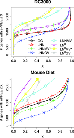
Figure 1: Comparison across methods of empirical ePPEE CDFs for DC3000 (top) and mouse diet (bottom) data.

The plots show substantial differences between the examined methods in the number of detected genes over a wide range of PPEE thresholds. For models with gene-specific error variances, incorporating uncertainty in estimated error variances greatly reduced the number of detected genes (LNNGV and LN³GV curves are lower than LNNMV* and LN³MV* curves, resp.). In the DC3000 data at a PPEE cutoff of 0.1, for example, the LNNMV, LNNMV*, and LNNGV methods would produce lists with 1983, 1498, and 893 genes, respectively. Incorporating gene effects greatly increased the number of detected genes (LN³, LN³MV*, and LN³GV curves are higher than LNN, LNNMV*, and LNNGV curves, resp.). In the mouse diet data at a PPEE cutoff of 0.1, for example, the LN³GV method identified almost three times as many DE genes as the LNNGV method (945 vs. 324 genes, resp.). These results indicate that differences between the methods’ ePPEEs are practically significant, and care should be taken when choosing among the suggested methods.

Constraints on time, money, material, and personnel resources limit the number of genes that researchers will follow up on with further study. Thus, the overlap between lists from each method containing a fixed number of the most significant genes is an important feature for assessing the similarity between methods’ results. Table 4 provides the size of pairwise intersections of lists containing the 200 most significant genes from each method for the DC3000 and mouse diet data sets, respectively. These results show substantial practical differences between rankings, as many lists overlap by roughly half their genes and most lists overlap by fewer than 150 genes.

Table 4: Overlap in lists of top 200 most significant DE genes for DC3000 (top) and mouse diet (bottom) data

Method	1	2	3	4	5	6	7
(1) GG	200
(2) LNN	187	200
(3) LNNMV	122	119	200
(4) LNNMV*	118	120	160	200
(5) LNNGV	130	127	185	162	200
(6) LN3	186	198	117	118	125	200
(7) LN3MV*	117	114	194	154	184	113	200
(8) LN3GV	077	081	137	149	133	079	135
(1) GG	200
(2) LNN	193	200
(3) LNNMV	108	107	200
(4) LNNMV*	125	124	152	200
(5) LNNGV	088	087	173	136	200
(6) LN3	193	197	109	124	089	200
(7) LN3MV*	093	092	181	134	184	094	200
(8) LN3GV	083	082	155	148	158	082	148

5 Simulation study

Here we briefly summarize our simulation study and its results. Detailed accounts of simulation procedures and results are presented in the supplementary material [Lund and Nettleton (2012)].

We conduct a variety of simulations to assess the accuracy and power of the considered methods. By “accuracy,” we refer to the property that for any given collection of genes the average estimated posterior probability for each pattern should closely match the proportion of genes in the collection that follow the given pattern. By “power,” we refer to a method’s ability to detect differential expression. We prefer the method that creates the largest list of genes for a given ePPEE threshold, provided that the method’s ePPEEs are accurate.

We simulated data from each of the five models (GG, LNN, LNNMV, LN³, and LN³MV) using the model parameters reported for the DC3000 data set in Table 3. In addition to these model-based simulations, we also conducted simulations using an HIV mRNA expression data set from the GEO website, named GDS1449. We analyzed each simulated data set with each method and recorded estimated posterior probabilities for each expression pattern for each gene.

The simulation results clearly support our claims that failing to distinctly model gene and gene-specific treatment effects reduces power and produces conservative results and that using point estimates of error variances produces liberal results. The LN³GV method stands out as the best method from these simulations. The LN³GV method was the only method to produce accurate ePPEEs in all simulation scenarios, and no method produced better average significance rankings (as seen in ROC curves) than those of the LN³GV method in any simulation scenario. The LN³GV method exhibited greater power than the LNNGV method, which was the only other method that did not produce liberal results in at least one simulation scenario.

6 Discussion

When modeling a data set that includes multiple observations from each of multiple genes, a conventional analysis would begin with a model that incorporates gene effects. One might decide to omit gene effects if, after looking, there was no evidence of gene effects or if results from an analysis were not affected by the omission of gene effects. We have demonstrated that gene effects are present in real data sets and provided generalizations of the methods based on lognormal two-level hierarchical models to include gene effects. These generalizations behave nearly identically to their two-level counterparts when analyzing data without gene effects and improve power and accuracy when data contain gene effects. These extensions serve as an example of how other hierarchical models that omit gene effects might be improved by more versatile modeling.

Using point estimates of gene-specific error variances without accounting for their uncertainty produces liberal ePPEEs. We have suggested a corrected approach that involves integration over an empirically estimated prior distribution for the error variances and demonstrated this adaptation yields accurate ePPEEs.

As noted in the Introduction, we have identified nearly a dozen methods that omit gene effects. There are far more methods in the microarray data analysis literature that do not suffer from this problem. Most published methods explicitly or implicitly include gene effects whose distribution is allowed to differ from the distribution of within gene treatment effects. Methods based on gene-specific linear models that make no attempt to borrow information across genes fall into this category, as do methods that borrow information across genes only for the purpose of improved error variance estimation. While we expect our LN³GV method to perform well when compared against the large collection of competing approaches, a broad comparison of methods is beyond the scope of this paper, and we make no claims of superiority here. Our main point is that the hierarchical modeling approach pioneered by Kendziorski et al. (2003) can be improved by the inclusion of both gene and gene-specific treatment effects. Given the influential nature of the original work of Kendziorski et al. (2003), we think this is an important point to make.

The development of the LNN and GG models by Kendziorski et al. (2003) represents groundbreaking work on the hierarchical modeling of gene expression data. We have shown how to improve on the original work by allowing for random gene effects and replacing gene-specific error variance point estimates without dramatically affecting computational costs. Adding random gene effects to a model increases the dimension of the parameter space across which the EM algorithm must optimize by one, but does not substantially increase computational costs. For any of the described methods, analyzing a data set with 5000 genes, 9 experimental units, and 4 expression patterns of interest takes less than 10 minutes using a single Linux machine and R code that calls a C routine to evaluate multivariate normal densities. We have developed the R package LN3GV (available at the CRAN webpage) to implement the LNNMV*, LNNGV, LN³, LN³MV*, and LN³GV methods discussed in this article. Throughout this paper, the GG, LNN, and LNNMV methods were implemented via the EBarrays package.

We have focused on the approach of Kendziorski et al. (2003) not only because of its influential nature but also because of its unique and elegant approach to inference for experiments with more than two treatments. The vast majority of competing approaches have been developed primarily for the case of two treatments. While it is easy to extend many of these methods to cover the case of more than two treatments, very few methods outside the Kendziorski et al. (2003) lineage provide an inherent natural strategy for classifying genes according to their pattern of expression across multiple treatments. Thus, we believe our efforts to improve the original work of Kendziorski et al. (2003) have been well spent.

Additional evidence supporting need for three-level hierarchy and simulation study details [doi]10.1214/12-AOAS535SUPP [url]http://lib.stat.cmu.edu/aoas/535/supplement.pdf .pdf The correlation across genes present in real microarray data makes directly testing the statistical significance of gene effect variance estimates intractable. We present a simulation study that demonstrates the gene effect variance estimates obtained when analyzing the DC3000 and mouse diet data sets are drastically greater than those that arise when analyzing data simulated without gene effects. We also provide detailed accounts of simulation procedures and results used to evaluate the considered methods. These simulations clearly support our claims regarding the importance of distinctly modeling gene and gene-specific treatment effects and accounting for uncertainty in error variance estimators.

References

- Baldi and Long (2001) {barticle}[author] \bauthor\bsnmBaldi, \bfnmPierre\binitsP. and \bauthor\bsnmLong, \bfnmAnthony D.\binitsA. D. (\byear2001). \btitleA Bayesian framework for the analysis of microarray expression data: Regularized -test and statistical inferences of gene changes. \bjournalBioinformatics \bvolume17 \bpages509–519. \bptokimsref \endbibitem
- Binder et al. (2004) {barticle}[author] \bauthor\bsnmBinder, \bfnmHans\binitsH., \bauthor\bsnmKirsten, \bfnmToralf\binitsT., \bauthor\bsnmLoeffler, \bfnmMarkus\binitsM. and \bauthor\bsnmStadle, \bfnmPeter F.\binitsP. F. (\byear2004). \btitleSensitivity of microarray oligonucleotide probes: Variability and effect of base composition. \bjournalThe Journal of Physical Chemistry B \bvolume108 \bpages18003–18014. \bptokimsref \endbibitem
- Cui et al. (2005) {barticle}[pbm] \bauthor\bsnmCui, \bfnmXiangqin\binitsX., \bauthor\bsnmHwang, \bfnmJ T Gene\binitsJ. T. G., \bauthor\bsnmQiu, \bfnmJing\binitsJ., \bauthor\bsnmBlades, \bfnmNatalie J.\binitsN. J. and \bauthor\bsnmChurchill, \bfnmGary A.\binitsG. A. (\byear2005). \btitleImproved statistical tests for differential gene expression by shrinking variance components estimates. \bjournalBiostatistics \bvolume6 \bpages59–75. \biddoi=10.1093/biostatistics/kxh018, issn=1465-4644, pii=6/1/59, pmid=15618528 \bptokimsref \endbibitem
- Irizarry et al. (2003) {barticle}[pbm] \bauthor\bsnmIrizarry, \bfnmRafael A.\binitsR. A., \bauthor\bsnmHobbs, \bfnmBridget\binitsB., \bauthor\bsnmCollin, \bfnmFrancois\binitsF., \bauthor\bsnmBeazer-Barclay, \bfnmYasmin D.\binitsY. D., \bauthor\bsnmAntonellis, \bfnmKristen J.\binitsK. J., \bauthor\bsnmScherf, \bfnmUwe\binitsU. and \bauthor\bsnmSpeed, \bfnmTerence P.\binitsT. P. (\byear2003). \btitleExploration, normalization, and summaries of high density oligonucleotide array probe level data. \bjournalBiostatistics \bvolume4 \bpages249–264. \biddoi=10.1093/biostatistics/4.2.249, issn=1465-4644, pii=4/2/249, pmid=12925520 \bptokimsref \endbibitem
- Jensen et al. (2009) {barticle}[mr] \bauthor\bsnmJensen, \bfnmShane T.\binitsS. T., \bauthor\bsnmErkan, \bfnmIbrahim\binitsI., \bauthor\bsnmArnardottir, \bfnmErna S.\binitsE. S. and \bauthor\bsnmSmall, \bfnmDylan S.\binitsD. S. (\byear2009). \btitleBayesian testing of many hypotheses many genes: A study of sleep apnea. \bjournalAnn. Appl. Stat. \bvolume3 \bpages1080–1101. \biddoi=10.1214/09-AOAS241, issn=1932-6157, mr=2750387 \bptokimsref \endbibitem
- Keleş (2007) {barticle}[mr] \bauthor\bsnmKeleş, \bfnmSündüz\binitsS. (\byear2007). \btitleMixture modeling for genome-wide localization of transcription factors. \bjournalBiometrics \bvolume63 \bpages10–21, 309. \biddoi=10.1111/j.1541-0420.2005.00659.x, issn=0006-341X, mr=2345570 \bptokimsref \endbibitem
- Kendziorski et al. (2003) {barticle}[author] \bauthor\bsnmKendziorski, \bfnmChristina M.\binitsC. M., \bauthor\bsnmNewton, \bfnmMichael\binitsM., \bauthor\bsnmLan, \bfnmH.\binitsH. and \bauthor\bsnmGould, \bfnmM. N.\binitsM. N. (\byear2003). \btitleOn parametric empirical Bayes methods for comparing multiple groups using replicated gene expression profiles. \bjournalStat. Med. \bvolume22 \bpages3899–3914. \bptokimsref \endbibitem
- Lo and Gottardo (2007) {barticle}[pbm] \bauthor\bsnmLo, \bfnmKenneth\binitsK. and \bauthor\bsnmGottardo, \bfnmRaphael\binitsR. (\byear2007). \btitleFlexible empirical Bayes models for differential gene expression. \bjournalBioinformatics \bvolume23 \bpages328–335. \biddoi=10.1093/bioinformatics/btl612, issn=1367-4811, pii=btl612, pmid=17138586 \bptokimsref \endbibitem
- Lönnstedt and Speed (2002) {barticle}[mr] \bauthor\bsnmLönnstedt, \bfnmIngrid\binitsI. and \bauthor\bsnmSpeed, \bfnmTerry\binitsT. (\byear2002). \btitleReplicated microarray data. \bjournalStatist. Sinica \bvolume12 \bpages31–46. \bidissn=1017-0405, mr=1894187 \bptokimsref \endbibitem
- Lund and Nettleton (2012) {barticle}[author] \bauthor\bsnmLund, \bfnmSteven P.\binitsS. P. and \bauthor\bsnmNettleton, \bfnmDan\binitsD. (\byear2012). \btitleSupplement to “The importance of distinct modeling strategies for gene and gene-specific treatment effects in hierarchical models for microarray data.” DOI:\doiurl10.1214/12-AOAS535SUPP. \bptokimsref \endbibitem
- Nettleton et al. (2006) {barticle}[author] \bauthor\bsnmNettleton, \bfnmDan\binitsD., \bauthor\bsnmHwang, \bfnmJ. T. Gene\binitsJ. T. G., \bauthor\bsnmCaldo, \bfnmRico A.\binitsR. A. and \bauthor\bsnmWise, \bfnmRoger P.\binitsR. P. (\byear2006). \btitleEstimating the number of true null hypotheses from a histogram of -values. \bjournalJ. Agric. Biol. Environ. Stat. \bvolume11 \bpages337–356. \bptokimsref \endbibitem
- Newton et al. (2004) {barticle}[pbm] \bauthor\bsnmNewton, \bfnmMichael A.\binitsM. A., \bauthor\bsnmNoueiry, \bfnmAmine\binitsA., \bauthor\bsnmSarkar, \bfnmDeepayan\binitsD. and \bauthor\bsnmAhlquist, \bfnmPaul\binitsP. (\byear2004). \btitleDetecting differential gene expression with a semiparametric hierarchical mixture method. \bjournalBiostatistics \bvolume5 \bpages155–176. \biddoi=10.1093/biostatistics/5.2.155, issn=1465-4644, pii=5/2/155, pmid=15054023 \bptokimsref \endbibitem
- Rossell (2009) {barticle}[mr] \bauthor\bsnmRossell, \bfnmDavid\binitsD. (\byear2009). \btitleGaga: A parsimonious and flexible model for differential expression analysis. \bjournalAnn. Appl. Stat. \bvolume3 \bpages1035–1051. \biddoi=10.1214/09-AOAS244, issn=1932-6157, mr=2750385 \bptokimsref \endbibitem
- Selinger et al. (2003) {barticle}[author] \bauthor\bsnmSelinger, \bfnmDouglas W.\binitsD. W., \bauthor\bsnmSaxena, \bfnmRini Mukherjee\binitsR. M., \bauthor\bsnmCheung, \bfnmKevin J.\binitsK. J., \bauthor\bsnmChurch, \bfnmGeorge M.\binitsG. M. and \bauthor\bsnmRoseno, \bfnmCarsten\binitsC. (\byear2003). \btitleGlobal RNA half-life analysis in Escherichia coli reveals positional patterns of transcript degradation. \bjournalGenome Research \bvolume13 \bpages216–223. \bptokimsref \endbibitem
- Smyth (2004) {barticle}[mr] \bauthor\bsnmSmyth, \bfnmGordon K.\binitsG. K. (\byear2004). \btitleLinear models and empirical Bayes methods for assessing differential expression in microarray experiments. \bjournalStat. Appl. Genet. Mol. Biol. \bvolume3 \bpagesArt. 3, 29 pp. (electronic). \biddoi=10.2202/1544-6115.1027, issn=1544-6115, mr=2101454 \bptokimsref \endbibitem
- Somel et al. (2008) {barticle}[pbm] \bauthor\bsnmSomel, \bfnmMehmet\binitsM., \bauthor\bsnmCreely, \bfnmHilliary\binitsH., \bauthor\bsnmFranz, \bfnmHenriette\binitsH., \bauthor\bsnmMueller, \bfnmUwe\binitsU., \bauthor\bsnmLachmann, \bfnmMichael\binitsM., \bauthor\bsnmKhaitovich, \bfnmPhilipp\binitsP. and \bauthor\bsnmPääbo, \bfnmSvante\binitsS. (\byear2008). \btitleHuman and chimpanzee gene expression differences replicated in mice fed different diets. \bjournalPLoS ONE \bvolume3 \bpagese1504. \biddoi=10.1371/journal.pone.0001504, issn=1932-6203, pmcid=2200793, pmid=18231591 \bptokimsref \endbibitem
- Wei and Li (2007) {barticle}[pbm] \bauthor\bsnmWei, \bfnmZhi\binitsZ. and \bauthor\bsnmLi, \bfnmHongzhe\binitsH. (\byear2007). \btitleA Markov random field model for network-based analysis of genomic data. \bjournalBioinformatics \bvolume23 \bpages1537–1544. \biddoi=10.1093/bioinformatics/btm129, issn=1367-4811, pii=btm129, pmid=17483504 \bptokimsref \endbibitem
- Wei and Li (2008) {barticle}[mr] \bauthor\bsnmWei, \bfnmZhi\binitsZ. and \bauthor\bsnmLi, \bfnmHongzhe\binitsH. (\byear2008). \btitleA hidden spatial–temporal Markov random field model for network-based analysis of time course gene expression data. \bjournalAnn. Appl. Stat. \bvolume2 \bpages408–429. \biddoi=10.1214/07–AOAS145, issn=1932-6157, mr=2415609 \bptokimsref \endbibitem
- Wright and Simon (2003) {barticle}[pbm] \bauthor\bsnmWright, \bfnmGeorge W.\binitsG. W. and \bauthor\bsnmSimon, \bfnmRichard M.\binitsR. M. (\byear2003). \btitleA random variance model for detection of differential gene expression in small microarray experiments. \bjournalBioinformatics \bvolume19 \bpages2448–2455. \bidissn=1367-4803, pmid=14668230 \bptokimsref \endbibitem
- Wu et al. (2007) {barticle}[mr] \bauthor\bsnmWu, \bfnmHaiyan\binitsH., \bauthor\bsnmYuan, \bfnmMing\binitsM., \bauthor\bsnmKaech, \bfnmSusan M.\binitsS. M. and \bauthor\bsnmHalloran, \bfnmM. Elizabeth\binitsM. E. (\byear2007). \btitleA statistical analysis of memory CD8 T cell differentiation: An application of a hierarchical state space model to a short time course microarray experiment. \bjournalAnn. Appl. Stat. \bvolume1 \bpages442–458. \biddoi=10.1214/07-AOAS118, issn=1932-6157, mr=2415750 \bptokimsref \endbibitem
- Yuan (2006) {barticle}[mr] \bauthor\bsnmYuan, \bfnmMing\binitsM. (\byear2006). \btitleFlexible temporal expression profile modelling using the Gaussian process. \bjournalComput. Statist. Data Anal. \bvolume51 \bpages1754–1764. \biddoi=10.1016/j.csda.2005.11.017, issn=0167-9473, mr=2307541 \bptokimsref \endbibitem
- Yuan and Kendziorski (2006a) {barticle}[mr] \bauthor\bsnmYuan, \bfnmMing\binitsM. and \bauthor\bsnmKendziorski, \bfnmChristina\binitsC. (\byear2006a). \btitleHidden Markov models for microarray time course data in multiple biological conditions. \bjournalJ. Amer. Statist. Assoc. \bvolume101 \bpages1323–1332. \biddoi=10.1198/016214505000000394, issn=0162-1459, mr=2307565 \bptokimsref \endbibitem
- Yuan and Kendziorski (2006b) {barticle}[mr] \bauthor\bsnmYuan, \bfnmMing\binitsM. and \bauthor\bsnmKendziorski, \bfnmChristina\binitsC. (\byear2006b). \btitleA unified approach for simultaneous gene clustering and differential expression identification. \bjournalBiometrics \bvolume62 \bpages1089–1098. \biddoi=10.1111/j.1541-0420.2006.00611.x, issn=0006-341X, mr=2297680 \bptokimsref \endbibitem