Abstract

We have conceived a supersymmetric Type II seesaw model at TeV scale, which has some additional particles consisting of scalar and fermionic triplet Higgs states, whose masses being around few hundred GeV. In this particular model, we have studied constraints on the masses of triplet states arising from the lepton flavor violating (LFV) processes, such as $\mu\to 3e$ and $\mu\to e\gamma$. We have analyzed the implications of these constraints on other observable quantities such as the muon anomalous magnetic moment and the decay patterns of scalar triplet Higgses. Scalar triplet Higgs states can decay into leptons and into supersymmetric fields. We have found that the constraints from LFV can effect these various decay modes.

Keywords: Supersymmetric models, Neutrino masses and mixing, Lepton flavor violation, Triplet Higgs states
PACS numbers: 12.60.Jv, 13.35.-r, 14.60.Pq

1 Introduction

The Standard Model (SM) has been a successful model and the only missing piece of it is the Higgs boson. In the recent experiment at the Large Hadron Collider (LHC), the discovery of a Higgs-like particle has been reported [1]. As of now the discovery at the LHC does not imply that it is a Higgs boson of the SM and it could even belong to the physics beyond the SM. On going studies at the LHC will confirm this in future. As for the physics beyond the SM, several motivations have been given [2]. The important motivations among these are the gauge hierarchy problem, smallness of neutrino masses, existence of dark matter, etc. Although there is a growing belief in the physics beyond the SM, the theoretical models in this category also have to deal with the constraints from the flavor violating processes. For a review on flavor violating processes, see Ref. [3]. The SM has been consistent with all the flavor violating processes due to the Glashow-Iliopoulos-Maiani cancellation mechanism, and this cancellation mechanism may not work in models of physics beyond the SM.

In this work, we have been motivated by arguments for physics beyond the SM [2], especially related to neutrino masses [4]. Among the various models for non-zero neutrino masses, Type II seesaw mechanism offers a viable model [5]. In this model, the scalar triplet Higgs with hypercharge $Y=1$ can give Majorana masses to neutrinos by acquiring a vacuum expectation value (vev) to the neutral component of the triplet Higgs. Due to the seesaw mechanism [5], the vev of neutral triplet Higgs can be as low as $\sim$ 1 eV, provided the masses of these states are ${\cal O}(10^{14})$ GeV. As a result of this, for ${\cal O}(1)$ Yukawa couplings the neutrino mass scale $m_{\nu}\sim$ 0.1 eV can be explained. Supersymmetry (SUSY) [6, 7] has been proposed to solve the gauge hierarchy problem and it is one of the main contenders for new physics. To explore the models among the physics beyond the SM, supersymmetrizing the Type II seesaw mechanism would be worth to do [8, 9]. In the supersymmetrized version of Type II seesaw model, both the scalar and fermionic states of triplet Higgses will have super heavy masses of ${\cal O}(10^{14})$ GeV. A positive aspect of having super heavy masses to triplet Higgs states is that the lepton flavor violating (LFV) processes in both the non-SUSY and SUSY versions of Type II seesaw model would be suppressed and they can be within the experimental limits. A negative point in these models is that these heavy triplet states cannot be produced at the LHC, and hence a direct detection is unlikely for the Type II seesaw mechanism. For indirect signals of super heavy triplet states, see Ref. [10]. Hence, for phenomenological studies at the LHC, we consider a specific version of SUSY Type-II seesaw model, where we conceive TeV scale masses for the triplet Higgs states.

In the Type II seesaw model, leptogenesis mechanism can be employed to explain the asymmetry between matter and anti-matter [8, 11]. In the non-SUSY version of Type II seesaw model, the recent indication of LHC experiment on the existence of Higgs boson [1] can also be accommodated [12]. In these models, the triplet Higgs states can induce LFV processes such as $\mu\to 3e$, $\tau\to 3\mu$, $\tau\to e2\mu$, etc at tree level, and at 1-loop level decays like $\mu\to e\gamma$, $\tau\to e\gamma$ and $\tau\to\mu\gamma$ can also happen. None of the above mentioned LFV decay processes have been observed in experiments and stringent experimental upper bounds have been put on the decay branching ratios of these processes [13]. In fact, in the SUSY version of Type II seesaw model, the above mentioned LFV processes can get additional radiative contributions which are induced by slepton fields. These additional contributions due to slepton fields also exist in the minimal supersymmetric standard model (MSSM). In the MSSM, the off-diagonal elements in soft masses of sleptons can generate LFV processes which are induced at 1-loop level. As a result of this, constraints on model parameters may be reduced in MSSM as compared to that in Type II seesaw model. Especially, we may expect stringent bounds in Type II seesaw model from processes such as $\mu\to 3e$ which take place at tree level.

In the literature, some work has already been done on the LFV processes in the non-SUSY version of Type II seesaw model at TeV scale [14, 15, 16]. Even in the SUSY version of Type II seesaw model at TeV scale, some work has been done in this direction [17]. However, in Ref. [17], a detailed study of constraints on model parameters arising from LFV processes has not been done. Moreover, in Ref. [17], the model has been motivated from high scale physics, and due to renormalization group effects, off-diagonal elements in the slepton mass matrices can become non-zero at low energy scale. As a result of this, processes like $\mu\to e\gamma$ can have additional contribution due to sletpon fields.

In this work, we have confined to the SUSY version of Type II seesaw model at the low energy scale and assume zero off-diagonal elements in charged slepton and sneutrino mass matrices. More precisely, we assume off-diagonal elements to be zero in the soft mass-squared terms and also in the soft $A$-terms of the slepton fields. This assumption makes our work to be different from that in Ref. [17]. Moreover, in our considered model, the LFV processes can happen only due to the non-diagonal Yukawa couplings of triplet Higgs field with the lepton doublets. Although we have neglected the contribution from slepton fields, the LFV processes in our work are clearly different from that of non-SUSY version of Type II seesaw model [14, 15, 16], since the fermionic partners of scalar triplet fields will give additional contribution to the LFV processes in our model.

The LFV processes in our model dominantly depend on neutrino Yukawa couplings and masses of triplet Higgs states. The Yukawa couplings can be determined from neutrino masses and mixing angles as well as from vev of scalar triplet Higgs. We will show later that the vev of scalar triplet Higgs can be around 1 eV in order to be compatible with neutrino oscillation data. Hence, by determining the Yukawa couplings, the experimental limits on LFV processes can put constraints on the masses of triplet Higgs states. We have studied implications of these constraints on other observable quantities such as the muon anomalous magnetic moment [18] and the decay patterns of scalar triplet Higgses. Since the triplet states have TeV scale masses, they can be pair produced at the LHC and their decay products give us experimental signals of this model. We have found that the constraints from LFV processes can effect the decay channels of these fields.

The organization of our paper is as follows. In the next section we give a brief description of SUSY version of Type-II seesaw model at TeV scale. In Sec. 3, we describe various possible LFV processes in this model and the expressions of their branching ratios. In Sec. 4, we have presented constraints due to the LFV processes on the masses of scalar and fermionic components of triplet Higgs states of this model. In the same section, we have also given results on the contribution of triplet states to the anomalous magnetic moment of the muon, $(g-2)_{\mu}$. In Sec. 5, we have described various decay channels of the scalar triplet Higgs states and their branching ratios. In Sec. 6, we have commented on phenomenological signals of this model in collider experiments. We conclude in Sec. 7. We have given total scalar potential of this model in Appendix A. Our conventions on neutralino and chargino mass matrices are described in Appendix B.

2 The Model

The gauge symmetry of the SUSY Type II seesaw model is SU(3)${}_{C}\times$SU(2)${}_{L}\times$U(1)_Y. The superpotential of this model can be written as [8, 9]

$$W = W_{\rm MSSM}+W_{\rm II},$$

$$W_{\rm MSSM} = Y_{u}^{jk}Q_{j}H_{u}D^{c}_{k}+Y_{d}^{jk}Q_{j}H_{d}D^{c}_{k}+Y_{e}^{jk}L_{j}H_{d}E^{c}_{k}+\mu H_{u}H_{d},$$

$$W_{\rm II} = Y_{\nu}^{jk}L_{j}i\sigma_{2}T_{1}L_{k}+\lambda_{1}H_{d}i\sigma_{2}T_{1}H_{d}+\lambda_{2}H_{u}i\sigma_{2}T_{2}H_{u}+M{\rm Tr}(T_{1}T_{2}).$$ (1)

In the above equation, $W_{\rm MSSM}$ is the superpotential of MSSM. Here, $j,k=1,2,3$ are the family indices and $\sigma_{j}$ are Pauli matrices. $Q$ and $L$ are the quark and lepton SU(2)_L doublet superfields, respectively. $U^{c}$, $D^{c}$ and $E^{c}$ are SU(2)_L singlet superfields which represent up-type, down-type quarks and charged lepton, respectively. $H_{u}$ and $H_{d}$ are the SU(2)_L doublet superfields with hypercharges $Y=\frac{1}{2}$ and $-\frac{1}{2}$, respectively. $\mu$ and $M$ are the only two mass parameters in the above equation. The terms in $W_{\rm II}$ contain SU(2)_L triplet superfields $T_{1}$ and $T_{2}$, whose hypercharges are $Y=1$ and $-1$, respectively. The forms of $T_{1}$ and $T_{2}$ are

$$T_{1}=\left(\begin{array}[]{cc}\frac{1}{\sqrt{2}}T_{1}^{+}&T_{1}^{++}\\ T_{1}^{0}&-\frac{1}{\sqrt{2}}T_{1}^{+}\end{array}\right),\quad T_{2}=\left(\begin{array}[]{cc}\frac{1}{\sqrt{2}}T_{2}^{-}&T_{2}^{0}\\ T_{2}^{--}&-\frac{1}{\sqrt{2}}T_{2}^{-}\end{array}\right).$$ (2)

The neutral part of scalar triplet Higgs in $T_{1}$ can acquire vev and it generates masses to neutrinos. The expression for neutrino mixing mass matrix is given below.

$$M_{\nu}^{jk}=2Y_{\nu}^{jk}v^{\prime}_{1},$$ (3)

where $\langle\phi_{1}^{0}\rangle=v^{\prime}_{1}$. The appearance of factor 2 in the above equation is due to the Majorana nature of neutrino fields. The vev of the neutral scalar part of $T_{2}$ is $\langle\phi_{2}^{0}\rangle=v^{\prime}_{2}$. From the naturalness of parameters we can expect $v^{\prime}_{1}\sim v^{\prime}_{2}$. Here, we use the convention that the scalar parts of triplet Higgs $T_{1}$ are denoted by $\phi_{1}$s and their supersymmetric counter parts are denoted by $\Delta_{1}$s. We follow the similar convention to denote the scalar and fermionic parts of $T_{2}$. To generate realistic neutrino masses, we can choose $Y_{\nu}\sim{\cal O}(1)$ and $v^{\prime}_{1}\sim$ 1 eV. By choosing $v_{1,2}^{\prime}\sim$ 1 eV, the upper limit ($\sim$ 1 GeV) on the vevs of scalar triplet Higgses, which arises from precision electroweak tests, can be satisfied. The Yukawa couplings can be uniquely determined in terms of neutrino masses and mixing angles, whose relations in a matrix format can be written as

$$Y_{\nu}=\frac{1}{2v^{\prime}_{1}}U^{*}_{\rm PMNS}M_{\rm diag}U^{\dagger}_{\rm PMNS},\quad M_{\rm diag}={\rm diag}(m_{1},m_{2},m_{3}),$$ (4)

where $m_{1,2,3}$ are the three neutrino mass eigenvalues and $U_{\rm PMNS}$ is the Pontecorvo-Maki-Nakagawa-Sakata unitary matrix. In the actual numerical analysis, we will see that either in the normal or inverted hierarchical mass pattern of neutrinos, the Yukawa couplings are $Y_{\nu}\sim 10^{-2}$ for $v^{\prime}_{1}\sim$ 1 eV. Unless there is a mechanism to justify the order 2 suppression in $Y_{\nu}$, we may take this as a natural value in the Type II seesaw mechanism.

In the non-SUSY version of Type II seesaw model, non-zero vev of scalar triplet Higgs arises due to the tri-linear coupling between triplet and doublet Higgs states [14, 15]. In the SUSY version of Type II seesaw model, this tri-linear coupling is equivalent to the $\lambda_{1,2}$-terms of Eq. (1). To realize the possibility of $v^{\prime}_{1,2}\sim$ 1 eV, we can take the dimensionless parameters $\lambda_{1,2}\sim{\cal O}(1)$ and the fermionic triplet Higgs mass $M\sim 10^{14}$ GeV [8, 9]. However, as explained before, in this case the masses of scalar and fermionic triplet Higgs states will be super heavy and a direct search for them at colliders is unlikely. Alternatively, we can consider another possibility where $\lambda_{1,2}\sim 10^{-10}$ and $M\sim$ 1 TeV [17]. In this later case, triplet Higgs states can be accessible at the on-going LHC experiment. The justification for the suppression of dimensionless couplings can be given if we embed the model in a high scale theory like supergravity [17]. Supergravity is a realistic scenario where supersymmetry breaking can be achieved through some gauge singlet fields known as hidden sector fields ($X$) [6, 7]. Hidden sector fields can break supersymmetry at an intermediate energy scale $\langle X\rangle=\Lambda\sim 10^{11}$ GeV, and as a result, the supersymmetric fields will have masses of the order of $\frac{\Lambda^{2}}{M_{P}}\sim$ 1 TeV. Here, $M_{P}$ is the Planck scale which is $\sim 10^{19}$ GeV. By embedding the model in a high scale theory, we may identify $\lambda_{1,2}\sim Y_{\nu}\frac{\langle X\rangle}{M_{P}}$, which gives the necessary suppression in the $\lambda_{1,2}$. Although a realistic construction for the above model can be made by embedding it in a high scale theory, it is beyond the scope of this work. We here, on the phenomenological grounds, consider a low energy setup of the above described SUSY Type II seesaw model.

The implications of supersymmetry breaking is to generate soft terms of scalar potential in the low energy regime. For full form of the scalar potential of this model, see Appendix A. Below we have given soft terms in the scalar potential which contain scalar triplet Higgs states.

$$V^{\rm triplet}_{\rm soft} = m_{\phi_{1}}^{2}Tr(\Phi_{1}^{\dagger}\Phi_{1})+m_{\phi_{2}}^{2}Tr(\Phi_{2}^{\dagger}\Phi_{2})+[B_{T}MTr(\Phi_{1}\Phi_{2})+(A_{\nu}Y_{\nu})^{jk}\tilde{L}_{j}i\sigma_{2}\Phi_{1}\tilde{L}_{k}$$ (5)

$$+(A_{\lambda_{1}}\lambda_{1})H_{d}i\sigma_{2}\Phi_{1}H_{d}+(A_{\lambda_{2}}\lambda_{2})H_{u}i\sigma_{2}\Phi_{2}H_{u}+{\rm h.c.}],$$

where the form of $\Phi_{1,2}$ is same as that of $T_{1,2}$ with its superfields being replaced by their scalar components. All the various mass parameters in the above equation would be at around 1 TeV. The term $Tr(\Phi_{1}\Phi_{2})$ gives mixing masses between the components of $\Phi_{1}$ and $\Phi_{2}$. In the following basis: $\psi_{++}=(\phi_{1}^{++},\left(\phi_{2}^{--}\right)^{*})^{\rm T}$, $\psi_{+}=(\phi_{1}^{+},\left(\phi_{2}^{-}\right)^{*})^{\rm T}$, $\psi_{0}=(\phi_{1}^{0},\left(\phi_{2}^{0}\right)^{*})^{\rm T}$, the mixing mass-squared terms of doubly charged, singly charged and neutral scalars can be written as

$$\psi_{++}^{\dagger}M_{++}^{2}\psi_{++},\quad\psi_{+}^{\dagger}M_{+}^{2}\psi_{+},\quad\psi_{0}^{\dagger}M_{0}^{2}\psi_{0}.$$ (6)

The form of $M_{++}^{2}$ is

$$M_{++}^{2}=\left(\begin{array}[]{cc}M^{2}+m_{\phi_{1}}^{2}+m_{++}^{2}&\left(B_{T}M\right)^{*}\\ B_{T}M&M^{2}+m_{\phi_{2}}^{2}-m_{++}^{2}\end{array}\right),$$ (7)

where $m_{++}^{2}=\frac{g^{2}-g^{\prime 2}}{2}\cos(2\beta)v^{2}$, which arises due to $D$-terms in the SUSY scalar potential (see Appendix A). By replacing $m_{++}^{2}$ with $m_{+}^{2}=-\frac{g^{\prime 2}}{2}\cos(2\beta)v^{2}$ and $m_{0}^{2}=-\frac{g^{2}+g^{\prime 2}}{2}\cos(2\beta)v^{2}$ in $M_{++}^{2}$, we get the corresponding forms for $M_{+}^{2}$ and $M_{0}^{2}$, respectively. Here, we have taken the electroweak scale as $v=174$ GeV and $\beta$ is defined as $\tan\beta=\langle H_{u}^{0}\rangle/\langle H_{d}^{0}\rangle$. $g,g^{\prime}$ are the gauge couplings of SU(2)_L and U(1)_Y gauge groups, respectively. Since the above mixing mass matrices ($M_{++}^{2}$, $M_{+}^{2}$, $M_{0}^{2}$) are hermitian, they can be diagonalized by unitary matrices which we denote by $U^{++}$, $U^{+}$ and $U^{0}$, respectively. For real parameters in the soft scalar potential, we can express $U^{++}$ in terms of model parameters, which is given below.

$$U^{++}=\left(\begin{array}[]{cc}\cos\theta^{++}&-\sin\theta^{++}\\ \sin\theta^{++}&\cos\theta^{++}\end{array}\right),\quad\sin 2\theta^{++}=\frac{2B_{T}M}{\sqrt{(m_{\phi_{1}}^{2}-m_{\phi_{2}}^{2}+2m_{++}^{2})^{2}+4(B_{T}M)^{2}}}.$$ (8)

Here, $\theta^{++}$ is the mixing angle between $\phi_{1}^{++}$ and $\left(\phi_{2}^{--}\right)^{*}$. Analogously, the elements of matrices $U^{+}$, $U^{0}$ can also be expressed in terms of model parameters.

Before concluding this section, we comment on the masses of fermionic triplet Higgs states. From the last term of $W_{\rm II}$, Eq. (1), we can see that the dominant contribution to the masses of these fields is $M$. However, after electroweak symmetry breaking, fermionic fields like $\Delta^{+}_{1}$, $\Delta^{-}_{2}$ and $\Delta^{0}_{1,2}$ will have some mixing masses with higgsinos, winos and bino. Because of this mixing, the neutralino and chargino mass matrices [6, 7] of MSSM will be extended to 6$\times$6 and 3$\times$3, respectively, in this model. The mixing masses can happen due to $\lambda_{1,2}$-terms of $W_{\rm II}$ and also due to gauge invariant kinetic $D$-terms of $T_{1,2}$ (See Sec. 5 for $D$-terms of $T_{1}$ and $D$-terms of $T_{2}$ can be analogously written). The corrections due to former terms are negligible due to the suppressed values of $\lambda_{1,2}$. The $D$-terms also give negligible corrections because these mixing masses are proportional to $v_{1,2}^{\prime}$. Since these corrections are $\sim$ 1 eV, we can safely take all the fermionic triplet Higgs states to be degenerate with a mass of $M$. As a result of this, in this work, we have taken both the neutralino and chargino mass matrices to be 4$\times$4 and 2$\times$2, respectively, which are described in Appendix B.

3 LFV processes

As described in Sec. 1, in our model, we assume vanishingly small off-diagonal elements in the soft mass-squared terms and also in $A$-terms of the slepton fields. As a result of this, in the lepton sector of our model, the Yukawa couplings in the first term of $W_{\rm II}$, Eq. (1), can only generate flavor changing processes, whose interaction terms in the Lagrangian are given below.

$${\cal L}=Y_{\nu}^{jk}\left[-2\nu_{L}^{j}\Delta_{1}^{0}\tilde{\nu}_{L}^{k}-\nu_{L}^{j}\nu_{L}^{k}\phi_{1}^{0}+\sqrt{2}\left(\nu_{L}^{j}\Delta^{+}_{1}\tilde{e}^{k}_{L}+e^{j}_{L}\Delta^{+}_{1}\tilde{\nu}_{L}^{k}+\nu_{L}^{j}e_{L}^{k}\phi^{+}_{1}\right)+2e_{L}^{j}\Delta^{++}_{1}\tilde{e}_{L}^{k}+e_{L}^{j}e_{L}^{k}\phi^{++}_{1}\right]+{\rm h.c.}$$ (9)

The last four terms in the above equation can drive LFV processes at tree level and and also at 1-loop level. Below we have described these processes.

3.1 LFV processes at tree level

The off-diagonal elements in the last term of Eq. (9) generate LFV processes at tree level such as $\mu^{-}\to e^{+}e^{-}e^{-}$, $\tau^{-}\to e^{+}e^{-}e^{-}$, $\tau^{-}\to\mu^{+}e^{-}\mu^{-}$, $\tau^{-}\to e^{+}\mu^{-}\mu^{-}$, $\tau^{-}\to e^{+}e^{-}\mu^{-}$, $\tau^{-}\to\mu^{+}e^{-}e^{-}$, $\tau^{-}\to\mu^{+}\mu^{-}\mu^{-}$. The experimental upper limit on $BR(\mu^{-}\to e^{+}e^{-}e^{-})$ is $10^{-12}$ [13] and the corresponding upper limits on the branching ratios of $\tau$-decays are about $\sim 10^{-8}$ [13]. These LFV processes are driven by the scalar field $\phi_{1}^{++}$. As explained in the previous section, in this model there is a mixing between $\phi_{1}^{++}$ and $\phi_{2}^{--}$. Hence, the contributions due to both these fields should be summed in the amplitudes of these processes. Below we have given expressions for branching ratios of the above mentioned decays.

$$BR(\mu^{-}\to e^{+}e^{-}e^{-}) = \frac{8|Y_{\nu}^{12}|^{2}|Y_{\nu}^{11}|^{2}}{g^{4}}m_{W}^{4}\left[\frac{|U^{++}_{11}|^{2}}{m_{\phi^{++}_{1}}^{2}}+\frac{|U^{++}_{12}|^{2}}{m_{\phi^{++}_{2}}^{2}}\right]^{2},$$

$$BR(\tau^{-}\to\ell_{j}^{+}\ell_{m}^{-}\ell_{l}^{-}) = S\frac{16|Y_{\nu}^{j3}|^{2}|Y_{\nu}^{lm}|^{2}}{g^{4}}m_{W}^{4}\left[\frac{|U^{++}_{11}|^{2}}{m_{\phi^{++}_{1}}^{2}}+\frac{|U^{++}_{12}|^{2}}{m_{\phi^{++}_{2}}^{2}}\right]^{2}BR(\tau^{-}\to\mu\bar{\nu}_{\mu}\nu_{\tau}),$$

where $m_{W}$, $m_{\phi^{++}_{1,2}}$ are the masses of $W$-boson and doubly charged $\phi$-fields, respectively. Here, $\ell_{1}=e$ and $\ell_{2}=\mu$ (Here, the muon field ($\mu$) is different from $\mu$-parameter of Eq. (1)). $S$ is a symmetric factor which equals to $\frac{1}{2}$ if $l=m$, otherwise it equals to 1. The branching ratio of $\tau^{-}\to\mu\bar{\nu}_{\mu}\nu_{\tau}$ is $\approx 0.17$. The elements of $Y_{\nu}$ can be computed from Eq. (4) by knowing the neutrino masses and mixing angles. The values of $U_{11}^{++}$ and $U_{12}^{++}$ can be computed from model parameters through Eq. (8), for real soft mass parameters.

In the previous section, we have motivated our model in such a way that in order to explain the smallness of neutrino masses, a natural parameter space is $v_{1}^{\prime}\sim$ 1 eV so that the elements of $Y_{\nu}$ are nearly unsuppressed. Hence, for this choice of parameter space, the above mentioned LFV processes can give lower bounds on the masses of doubly charged scalar fields. As explained before that due to similarity in the form of matrices $M_{++}^{2},M_{+}^{2},M_{0}^{2}$, the above mentioned bounds on the doubly charged fields will translate into similar lower bounds on the masses of singly charged and neutral scalar triplet fields. Hence, we can conclude that in our scenario the LFV processes at tree level can constrain the masses of scalar components of the triplet states.

3.2 Radiative LFV processes

The last four terms of Eq. (9) can generate LFV processes at 1-loop level. These are $\mu\to e\gamma$, $\tau\to e\gamma$ and $\tau\to\mu\gamma$. The experimental upper limit on $BR(\mu\to e\gamma)$ is $2.4\times 10^{-12}$ at 90$\%$ C.L. [20], and the corresponding upper limits on $BR(\tau\to e\gamma,\mu\gamma)$ are about $10^{-8}$ [13]. We will show later that the upper bounds on the branching ratios of radiative LFV processes can put lower bounds on the masses of fermionic triplet Higgs states.

Let us consider the decay process $\ell_{j}(p)\to\ell_{i}(p^{\prime})+\gamma(q)$, which takes place at one loop level. Here, $i,j=1,2,3$ are family indices. $\ell_{i}$ and $\ell_{j}$ are some negatively charged leptons with 4-momenta $p^{\prime}$ and $p$, respectively. The outgoing $\gamma$ has 4-momenta $q=p-p^{\prime}$. Below we present the decay width for $\ell_{j}(p)\to\ell_{i}(p^{\prime})+\gamma(q)$, where we have neglected the left-right mixing of charged sleptons. The decay width of the above process is governed by the amplitude which has the following form, where there is no summation on the indices $i,j$.

$$i{\cal M}=ie\bar{u}_{i}(p^{\prime})\left[A^{ij}_{R}\frac{1+\gamma_{5}}{2}+A^{ij}_{L}\frac{1-\gamma_{5}}{2}\right]i\sigma^{\mu\nu}q_{\nu}\epsilon_{\mu}^{*}(q)u_{j}(p).$$ (11)

Here, $u_{i}$ and $u_{j}$ are the Dirac spinors of the charge leptons $\ell_{i}$ and $\ell_{j}$, respectively, and $\epsilon_{\mu}(q)$ is the polarization of photon. The forms of $A^{ij}_{R}$ and $A^{ij}_{L}$ are given below, where there is no summation on the indices $i,j$.

$$A^{ij}_{R}=A_{ij}m_{\ell_{j}},\quad A^{ij}_{L}=A_{ij}m_{\ell_{i}},$$

$$A_{ij}=\sum_{k=1}^{3}\left\{-\frac{\left(Y_{\nu}^{ki}\right)^{*}Y_{\nu}^{kj}}{12\pi^{2}}\left[\left(\frac{|U^{++}_{11}|^{2}}{m_{\phi^{++}_{1}}^{2}}+\frac{|U^{++}_{12}|^{2}}{m_{\phi^{++}_{2}}^{2}}\right)+\frac{1}{8}\left(\frac{|U^{+}_{11}|^{2}}{m_{\phi^{+}_{1}}^{2}}+\frac{|U^{+}_{12}|^{2}}{m_{\phi^{+}_{2}}^{2}}\right)\right]\right.$$

$$\left.+\frac{\left(Y_{\nu}^{ki}\right)^{*}Y_{\nu}^{kj}}{16\pi^{2}M^{2}}\left[2f_{1}(x_{k}^{++})+4f_{2}(x_{k}^{++})+f_{2}(x_{k}^{+})\right]\right\},$$ (12)

$$x_{k}^{++}=\frac{m_{\tilde{l}_{k}}^{2}}{M^{2}},\quad x_{k}^{+}=\frac{m_{\tilde{\nu}_{k}}^{2}}{M^{2}},$$

$$f_{1}(x)=\frac{1}{(1-x)^{4}}\left[\frac{1}{3}+\frac{x}{2}-x^{2}+\frac{x^{3}}{6}+x\log(x)\right],$$

$$f_{2}(x)=\frac{1}{(1-x)^{4}}\left[\frac{1}{6}-x+\frac{x^{2}}{2}+\frac{x^{3}}{3}-x^{2}\log(x)\right].$$ (13)

Here, $m_{\ell_{i}}$, $m_{\tilde{l}_{k}}$ and $m_{\tilde{\nu}_{k}}$ are the masses of charged lepton, charged slepton and sneutrino fields, respectively. The decay width of $\mu\to e\gamma$ is given by

$$\Gamma(\mu\to e\gamma)=\frac{e^{2}}{16\pi}\left(|A^{12}_{R}|^{2}+|A^{12}_{L}|^{2}\right)\frac{(m_{\mu}^{2}-m_{e}^{2})^{3}}{m_{\mu}^{3}}.$$ (14)

After neglecting the electron mass, the branching ratio of $\mu\to e\gamma$ is

$$Br(\mu\to e\gamma)=\frac{\Gamma(\mu\to e\gamma)}{\Gamma(\mu\to e\bar{\nu}_{e}\nu_{\mu})}=\frac{48\alpha\pi^{3}}{G_{F}^{2}}\left(A_{12}\right)^{2},$$ (15)

where $\alpha=\frac{e^{2}}{4\pi}$ and $G_{F}=1.166\times 10^{-5}$ GeV^-2. The branching ratio of $\tau\to e\gamma$ can be computed from

$$Br(\tau\to e\gamma)=\frac{48\alpha\pi^{3}}{G_{F}^{2}}\left(A_{13}\right)^{2}BR(\tau\to\mu\bar{\nu}_{\mu}\nu_{\tau}).$$ (16)

In the above expression by replacing $A_{13}\to A_{23}$, we can get the expression for branching ratio of $\tau\to\mu\gamma$. In these expressions we have applied the approximation $m_{\mu}^{2}\ll m_{\tau}^{2}$.

The expression for the muon anomalous magnetic moment, $(g-2)_{\mu}$ [18], can be found from the same amplitude of $\ell_{j}\to\ell_{i}+\gamma$, which is described above. By identifying $\ell_{i}=\ell_{j}=\mu$, the necessary amplitude for the $(g-2)_{\mu}$ can be written as

$$i{\cal M}=ie\bar{u}_{\mu}(p^{\prime})\left[A^{22}_{R}\frac{1+\gamma_{5}}{2}+A^{22}_{L}\frac{1-\gamma_{5}}{2}\right]i\sigma^{\mu\nu}q_{\nu}\epsilon^{*}_{\mu}(q)u_{\mu}(p),$$ (17)

where $u_{\mu}$ is the Dirac spinor of the muon. From the above amplitude, we can read the contribution to the $(g-2)_{\mu}$ due to the triplet Higgs states, whose expression is given below.

$$\Delta a^{\rm T}_{\mu}=\left(A^{22}_{R}+A^{22}_{L}\right)2m_{\mu}=2A_{22}m_{\mu}^{2}.$$ (18)

Here we comment on our results on the decay branching ratios of flavor changing processes with the previously work done in the non-SUSY [15] and SUSY [17] versions of the Type II seesaw model. The LFV processes at tree level are driven by the doubly charged scalar triplet fields. In the limit $B_{T}=0$, the mixing between the fields $\phi^{++}_{1},\phi^{--}_{2}$ will vanish and the branching ratios of these processes reduce to the expressions as they are given in Ref. [15]. The amplitudes for radiative decay processes, such as $\mu\to e\gamma$, get contribution from scalar (1st line of Eq. (12)) as well as from fermionic (2nd line of Eq. (12)) components of triplet Higgs. Again, in the limit $B_{T}=0$, the contribution from first line of Eq. (12) reduces to the expression as it is given in Ref. [15], while the fermionic triplet contribution of Eq. (12) has a similar form to the corresponding expression given in Ref. [17]. However, the sign proportional to the $f_{1}(x^{++}_{k})$-term is given with a minus sign in Ref. [17].

4 Constraints from the LFV processes

Before explaining constraints from the LFV processes, we here make brief comments on relaxing constraints from the tree level LFV processes. Among these, we can expect stringent limits from $BR(\mu\to 3e)$. To suppress limits from $BR(\mu\to 3e)$, we can fine tune the Yukawa couplings $Y_{\nu}^{12},Y_{\nu}^{11}$ to be vanishingly small [14, 15, 16]. However, it has been reported in Ref. [21] that to achieve $Y_{\nu}^{12}=0$, the neutrino mixing angle $\theta_{13}$ will have to be too small which is not consistent with the recently measured value of $\theta_{13}$ at the Double Chooz, Daya Bay and RENO experiments [22]. Nevertheless, here our motivation is that we choose generic values for neutrino masses and mixing angles, and study bounds on the masses of triplet Higgs states.

The six neutrino Yukawa couplings in this model, Eq. (4), are determined by the neutrino masses and mixing angles. The mixing angles are incorporated in the unitary matrix $U_{\rm PMNS}$, and we have parametrized this matrix according to the convention in Ref. [13]. Here, without loss of generality, we have chosen the CP violating phase $\delta$ and the two Majorana phases to be zero. We have taken the neutrino mass-squared differences as [23]: $m_{\rm solar}^{2}=m_{2}^{2}-m_{1}^{2}=7.62\times 10^{-5}~{}{\rm eV}^{2}$ and $m_{\rm atm}^{2}=m_{3}^{2}-m_{1}^{2}=2.53(-2.4)\times 10^{-3}~{}{\rm eV}^{2}$. Here, the term in bracket gives inverted hierarchical mass pattern for neutrinos. To be consistent with the above neutrino mass-squared values, we can choose three different hierarchical mass patterns, which are described below.

$${\rm Normal~{}hierarchy~{}(NH)}:m_{1}=0,\quad m_{2}=m_{\rm solar},\quad m_{3}=m_{\rm atm}$$

$${\rm Inverted~{}hierarchy~{}(IH)}:m_{3}=0,\quad m_{1}=m_{\rm atm},\quad m_{2}=\sqrt{m_{\rm solar}^{2}+m_{1}^{2}}$$

$${\rm Degenerate~{}Neutrinos~{}(DN)}:m_{1}=0.3~{}{\rm eV},\quad m_{2}=\sqrt{m_{\rm solar}^{2}+m_{1}^{2}},\quad m_{3}=\sqrt{m_{\rm atm}^{2}+m_{1}^{2}}$$

As for the mixing angles, we have taken them as: $\sin\theta_{12}=\frac{1}{\sqrt{3}}$, $\sin\theta_{23}=\frac{1}{\sqrt{2}}$ and $\sin\theta_{13}=0.1737$. Here $\theta_{13}=10^{\rm o}$ and the other two angles are fitted to the tri-bimaximal values [24]. All these values are consistent with the global fitting to the neutrino oscillation data, done in Ref. [23].

After determining the Yukawa couplings, $BR(\mu\to 3e)$ can put limits on $m_{\phi^{++}_{1}}$ and $m_{\phi^{++}_{2}}$. However in this analysis, we also have to know the values of $U^{++}_{11},U^{++}_{12}$. It can be seen from Eq. (8) that for generic SUSY parameter space, where $B_{T}M\sim M^{2}\sim m^{2}_{\phi_{1,2}}$, $U^{++}_{11},U^{++}_{12}\sim{\cal O}(1)$. Hence the lower bound on $m_{\phi^{++}_{1}}$ would be nearly the same as on $m_{\phi^{++}_{2}}$. Alternatively, to simplify this task, we may choose the soft parameters $B_{T}=0$ and $m_{\phi_{1}}^{2}\sim m_{\phi_{2}}^{2}$. In this case, $\phi^{++}_{1}$ and $\phi^{--}_{2}$ will be decoupled away from each other and we get lower bound on $m_{\phi^{++}_{1}}$ from $BR(\mu\to 3e)$. From Eq. (7), it can be noticed that for $\tan\beta\sim 10$, the electroweak corrections to the triplet Higgses would be at most $\sim$10 GeV. Hence, the lower bound on $m_{\phi^{++}_{1}}$ will put nearly the same lower bound on $m_{\phi^{++}_{2}}$. In fact, the arguments given below Eq. (7) would suggest that similar amount of lower bounds will apply on the singly charged and neutral triplet scalar fields. Hence from the above argument of simplicity we choose $B_{T}=0$ in this section.

In Tab. 1 we have presented lower bounds on the mass of $\phi^{++}_{1}$ which arise from $BR(\mu\to 3e)<10^{-12}$.

	NH	IH	DN
$v^{\prime}_{1}$	$m_{\phi^{++}_{1}}$	$m_{\phi^{++}_{1}}$	$m_{\phi^{++}_{1}}$
1.0 eV	631.8 GeV	1.71 TeV	1.32 TeV
0.5 eV	1.26 TeV	3.41 TeV	2.64 TeV
0.1 eV	6.32 TeV	17.07 TeV	13.21 TeV

Table 1: Lower bounds on the mass of $\phi^{++}_{1}$ arising from $BR(\mu\to 3e)<10^{-12}$, for different values of $v^{\prime}_{1}$. These lower bounds are given in all the three hierarchical mass patterns of neutrinos.

We have checked that the lower bounds on $m_{\phi^{++}_{1}}$ due to $BR(\mu\to 3e)<10^{-12}$ will simultaneously satisfy the experimental limits on the branching ratios of $\tau$ decays such as $\tau\to 3e$, $\tau\to e2\mu$, etc. The lower bounds in Tab. 1 can be compared to the lower bound of about 400 GeV on $m_{\phi^{++}}$ by the CMS collaboration of the LHC experiment [25]. From Tab. 1, we can notice that the lower bounds in the case of NH are much lower compared to that in IH and DN cases. The product $Y_{\nu}^{12}\times Y_{\nu}^{11}$, which determines $BR(\mu\to 3e)$, is lower in the case of NH as compared to that in IH and DN cases. However, if we look at numerical values, for $v^{\prime}_{1}=$ 1.0 eV, in both the NH and IH cases the elements of $Y_{\nu}$ are $\sim 10^{-3}$, whereas, in the case of DN the diagonal and off-diagonal elements of $Y_{\nu}$ are around 0.1 and $10^{-4}$ respectively. The lower bound on $m_{\phi^{++}_{1}}$ increases with decreasing $v^{\prime}_{1}$, since from Eq. (4) we see that $Y_{\nu}\sim\frac{1}{v^{\prime}_{1}}$. In fact, from Tab. 1, for $v^{\prime}_{1}=$ 0.1 eV, the masses of scalar triplets are so high that there is very less chance of their detection at the current LHC experiment.

Now, by inputting the lower bounds of the masses of scalar triplet Higgses in the radiative LFV processes, such as $\mu\to e\gamma$, we can derive lower bounds on the masses of fermionic triplet Higgs states. From the expressions of decay branching ratios of $\ell_{j}\to\ell_{i}\gamma$, which are given in the previous section, we can notice that the masses of charged slepton and sneutrino fields will also contribute to these radiative processes. For simplicity, we have chosen degenerate masses for the three charged sleptons ($m_{\tilde{l}}$) and for the three sneutrino fields ($m_{\tilde{\nu}}$). Regarding the masses of scalar components of triplet Higgses, as explained previously, the electroweak corrections can be at most $\sim$10 GeV, and so in our numerical analysis we have taken $m_{\phi^{++}_{1}}\approx m_{\phi^{+}_{1}}$. Moreover, in our analysis, we have fixed the values of $m_{\phi^{++}_{1}}$ to the lower limits as they are given in Tab. 1, and we comment below on what may happen if we increase its value. From the experimental limits on radiative LFV decays [13, 20], we expect stringent constraints on model parameters from $BR(\mu\to e\gamma)$. As a result of this, in the analysis, for some fixed values of $m_{\tilde{l}}$ and $m_{\tilde{\nu}}$, we first check if the constraints from $BR(\tau\to e\gamma,\mu\gamma)$ are satisfied and then compute $BR(\mu\to e\gamma)$ as a function of fermionic triplet Higgs mass, $M$.

In Fig. 1, in the case of NH, we have given constraints on $M$ from the above mentioned radiative LFV processes.

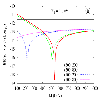
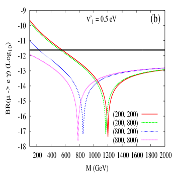
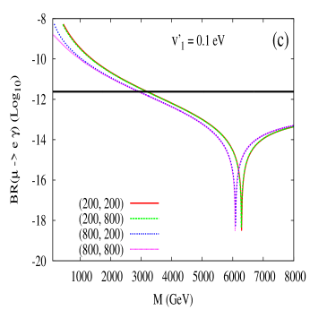
Figure 1: In the normal hierarchy, $\log_{10}(BR(\mu\to e\gamma))$ has been plotted against the mass of fermionic triplet Higgs. The three plots are for $v^{\prime}_{1}=$ 1.0, 0.5 and 0.1 eV. In each of these plots, the four lines are for different values of charged slepton and sneutrino masses, which are represented in the format $(m_{\tilde{l}},m_{\tilde{\nu}})$ in GeV units. The horizontal line in these plots indicate $BR(\mu\to e\gamma)=2.4\times 10^{-12}$, and the area below this line is allowed. The lower limit on the x-axis is 100 GeV.

In Fig. 1(a), we have fixed $v^{\prime}_{1}=1.0$ eV and plotted $BR(\mu\to e\gamma)$ versus $M$ for four different combinations of $(m_{\tilde{l}},m_{\tilde{\nu}})$. Among these four different combinations, $(m_{\tilde{l}},m_{\tilde{\nu}})$ = (200 GeV, 200 GeV) has given stringent lower limit on $M$ which is about 200 GeV. The next stringent limit on $M$ has come from the other combination of $(m_{\tilde{l}},m_{\tilde{\nu}})$ = (200 GeV, 800 GeV), which sets $M\geq$ 180 GeV. Whereas, the other two combinations such as $(m_{\tilde{l}},m_{\tilde{\nu}})$ = (800 GeV, 200 GeV) and (800 GeV, 800 GeV) have put no limits on $M$. In Figs. 1(b) and 1(c), we have decreased $v^{\prime}_{1}$ to 0.5 eV and 0.1 eV, respectively. In these two plots we can observe that the lower limits on $M$ will be stringent from the combination $(m_{\tilde{l}},m_{\tilde{\nu}})$ = (200 GeV, 200 GeV) as compared to the other three combinations which we have mentioned above. The stringent lower limits on $M$ in Figs. 1(b) and 1(c) are about 550 GeV and 3190 GeV, respectively. From these observations we can conclude that $BR(\mu\to e\gamma)$ has greater sensitivity on $m_{\tilde{l}}$ as compared to that on $m_{\tilde{\nu}}$, and lower the value of $m_{\tilde{l}}$ the greater would be the lower limit on $M$. The lower bounds on $M$ increases with decreasing $v^{\prime}_{1}$, since the elements of $Y_{\nu}$ will increase. Another point to notice from the plots of Fig. 1 is that $BR(\mu\to e\gamma)$ decreases with $M$ and goes to a dip at a certain value of $M$, and then for a large value of $M$ it becomes saturate. The reason for this is as follows. From the amplitude of the process $\ell_{j}\to\ell_{i}+\gamma$, Eq. (12), we can notice that there is a relative minus sign between the contributions of scalar and fermionic components of triplet Higgs. Moreover, as explained before, in the numerical analysis, we have fixed the contribution from scalar components by fixing their masses. Hence, due to the above mentioned relative minus sign, at a certain value of $M$ the amplitude for $\ell_{j}\to\ell_{i}+\gamma$ will become zero, and then goes to the saturation for large value of $M$, since the amplitude is $\propto\frac{1}{M^{2}}$. Since we have fixed the masses of scalar components of triplet Higgs to the lower limits presented in Tab. 1, we here comment on what happens if we increase their masses. Again, due to the above mentioned relative minus sign, we can easily understand that the lower bound on $M$ increases with $m_{\phi_{1}^{++}}$. A final comment on the plots of Fig. 1 is that the bounds from the decays $\tau\to e\gamma,\mu\gamma$ can be seen in the case of $v^{\prime}_{1}$ = 0.1 eV but not in the cases of $v^{\prime}_{1}$ = 1.0 eV and 0.5 eV. In Fig. 1(c) there are no points for $M<$ 450 GeV and for $(m_{\tilde{l}},m_{\tilde{\nu}})$ = (200 GeV, 200 GeV), because these points are are not satisfied by the experimental limits on $Br(\tau\to e\gamma,\mu\gamma)$.

In Figs. 2(a) and 2(b) we have given constraints on $M$ in the cases of IH and DN, respectively.

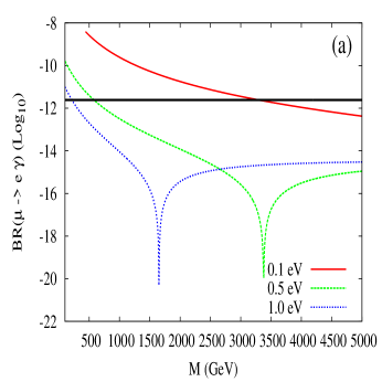
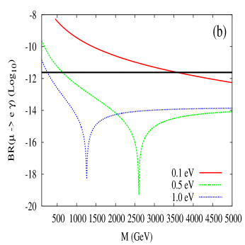
Figure 2: In the left and right plots, $\log_{10}(BR(\mu\to e\gamma))$ has been plotted against the mass of fermionic triplet Higgs, in the cases of IH and DN, respectively. In both of these plots, charged slepton and sneutrino masses have been taken to be 200 GeV each. The three lines in each of the above plots are for different values of $v^{\prime}_{1}$ in eV units. The horizontal line in these plots indicate $BR(\mu\to e\gamma)=2.4\times 10^{-12}$, and the area below this line is allowed. The lower limit on the x-axis is 100 GeV.

In both of these cases, we have noticed that the dependence of $BR(\mu\to e\gamma)$ on the $m_{\tilde{l}}$ and $m_{\tilde{\nu}}$ is same as that described around Fig. 1. Hence, in both the plots of Fig. 2 we have fixed $m_{\tilde{l}}$ and $m_{\tilde{\nu}}$ to a lower value of 200 GeV, which should give stringent limits on $M$. We have varied $v^{\prime}_{1}$ in both the plots of Fig. 2. In the case of IH(DN) the lower limits on $M$ for $v^{\prime}_{1}$ = 1.0 eV, 0.5 eV and 0.1 eV are 210(240) GeV, 570(630) GeV, 3300(3580) GeV, respectively. Comparing these limits with the limits presented in the previous paragraph, the lower bound on $M$ in the case of IH are intermediate between NH and DN cases, and that the limits in the case of DN are stronger. In both of the plots of Fig. 2, we can notice constraints arising from $BR(\tau\to e\gamma,\mu\gamma)$ in the case of $v^{\prime}_{1}$ = 0.1 eV, where points for $M<$ 450 GeV are not satisfied by them.

In Tab. 2, we have summarized the lower limits on $M$ for different values of $v^{\prime}_{1}$ and in different hierarchical mass patterns of neutrinos.

	NH	IH	DN
$v^{\prime}_{1}$	$M$	$M$	$M$
1.0 eV	204 GeV	216 GeV	248 GeV
0.5 eV	557 GeV	579 GeV	639 GeV
0.1 eV	3.20 TeV	3.31 TeV	3.59 TeV

Table 2: Lower bound on $M$ arising from $BR(\mu\to e\gamma)<2.4\times 10^{-12}$, for different values of $v^{\prime}_{1}$. These lower bounds are given in all the three hierarchical mass patterns of neutrinos and for $(m_{\tilde{l}},m_{\tilde{\nu}})$ = (200 GeV, 200 GeV). See text, for more details.

These lower bounds are given for $(m_{\tilde{l}},m_{\tilde{\nu}})$ = (200 GeV, 200 GeV), in which case the limits on $M$ would be stringent. Moreover, while computing the lower bounds on $M$, we have fixed $m_{\phi_{1}^{++}}\approx m_{\phi_{1}^{+}}$ to the values mentioned in Tab. 1. By comparing the limits in Tab. 1 with that in Tab. 2, we can notice that the lower bounds on $M$ are less than that on $m_{\phi^{++}_{1}}$. The reason for this is that the bounds on $M$ and $m_{\phi^{++}_{1}}$ are coming from LFV processes induced at 1-loop level and tree level, respectively.

After discussing the limits on the masses of scalar and fermionic triplet Higgs states, which arise from LFV processes, we now discuss the contribution of these triplet fields to the muon anomalous magnetic moment, $(g-2)_{\mu}$ [18]. The current discrepancy between the SM and the experimental value of $(g-2)_{\mu}$ can be taken as $\Delta a_{\mu}=a_{\mu}^{\rm EXP}-a_{\mu}^{\rm SM}=(29\pm 9)\times 10^{-10}$ [18], where $a_{\mu}=\frac{(g-2)_{\mu}}{2}$. The $(g-2)_{\mu}$ is a good observable quantity in the study of new physics. In our model of SUSY Type II seesaw at TeV scale, neutralino$-$charged slepton and chargino$-$sneutrino loops will give contribution to the $(g-2)_{\mu}$ [26], and the above discrepancy can be easily fitted. On top of this loop contribution, the scalar and fermionic triplet Higgs states will also give additional contribution to the $(g-2)_{\mu}$, which is given in Eq. (18). From the relation in Eq. (18), we can notice that the scalar and fermionic triplet Higgs states give negative and positive contributions, respectively. Since the current discrepancy in $\Delta a_{\mu}$ is strictly positive, the non-SUSY Type II seesaw model, where the contribution is from scalar triplet Higgses, cannot explain this discrepancy [16]. In our present model, the fermionic triplet Higgs states give positive contribution, so it is interesting to see how large can this contribution be to the $(g-2)_{\mu}$. The contribution of $\Delta a^{\rm T}_{\mu}$, Eq. (18), greatly depends on the sizes of Yukawa couplings. As mentioned before, in the cases of NH and IH, for $v^{\prime}_{1}$ = 0.1 eV the Yukawa couplings are $\sim 10^{-2}$. Since these couplings are very small, we do not expect appreciable amount to $\Delta a^{\rm T}_{\mu}$, in the cases of NH and IH. Whereas, in the case of DN, the diagonal and off-diagonal Yukawa couplings are around 1.5 and $\sim 10^{-3}$, respectively, for $v^{\prime}_{1}$ = 0.1 eV. Hence, at least from the diagonal Yukawa coupling $Y_{\nu}^{22}$ we can expect an enhancement to the $\Delta a^{\rm T}_{\mu}$.

In Fig. 3 we have plotted $\Delta a^{\rm T}_{\mu}$ versus $M$ in the case of DN.

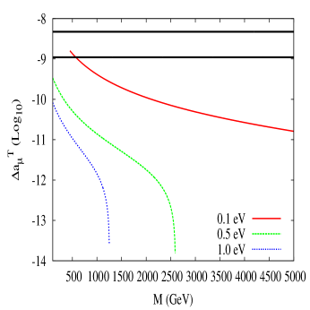
Figure 3: The contribution of triplet Higgs states to $\log_{10}(\Delta a_{\mu}^{\rm T})$ has been plotted against $M$, in the case of DN. The masses of charged slepton and sneutrino have been fixed to 200 GeV each. The three lines in this plot are for different values of $v^{\prime}_{1}$, expressed in eV units. The horizontal lines represent the lower and upper end of the $2\sigma$ limit of $\Delta a_{\mu}$, see text for details.

In this figure, we have kept the masses of scalar triplet Higgses to the lower limits of Tab. 1, and also included the constraints from $\tau\to e\gamma,\mu\gamma$. The lower and upper horizontal lines in Fig. 3 represent the 2$\sigma$ limits of the discrepancy in $\Delta a_{\mu}$, which can be taken as $1.1\times 10^{-9}$ and $4.7\times 10^{-9}$, respectively. The area between these lines is allowed from the $(g-2)_{\mu}$. For $v^{\prime}_{1}$ = 1.0 eV and 0.5 eV the Yukawa couplings are so small that the discrepancy in the $(g-2)_{\mu}$ cannot be fitted by the triplet Higgses. Whereas for $v^{\prime}_{1}$ = 0.1 eV, there is a chance to fit this discrepancy for a low value of $M$. However, the constraint from $\mu\to e\gamma$ puts a lower limit on $M$ to be around 3600 GeV. Hence, after including the constraints from LFV processes the maximum contribution to the $(g-2)_{\mu}$ from triplet Higgses in this model is found to be $3.4\times 10^{-11}$ for $v^{\prime}_{1}$ = 0.1 eV, or 0.5 eV, or 1.0 eV. This contribution is two orders smaller than the required amount. Hence, in the SUSY Type II seesaw model, the discrepancy in $(g-2)_{\mu}$ can be fitted with the loop induced diagrams of neutralino-charged slepton and chargino-sneutrino. The reason for discontinuity of lines in Fig. 3 is that after a certain large value of $M$ the scalar contribution to $\Delta a^{\rm T}_{\mu}$ will be dominant which is negative, and we have plotted $\Delta a^{\rm T}_{\mu}$ in the units of $\log_{10}$. The amount of this negative value is so small that it gives negligible contribution to the $(g-2)_{\mu}$.

5 Decays of scalar triplet Higgses

The detection of components of triplet Higgs at the LHC can give validity to our model. At the LHC or an $e^{+}e^{-}$ collider, through the $\gamma$ and $Z$ mediated processes, both the charged as well as the neutral components of triplet Higgses can be pair produced. The production process for fermionic triplet Higgs states ($\Delta$s) at a collider experiment is similar to the corresponding production of charginos of the MSSM. For the production of scalar triplet Higgses at collider experiments, see Refs. [28, 29, 30]. Here, we study the decay products of scalar triplet Higgses, through which the detection of these fields can be done at collider experiments. The decays of fermionic triplet Higgs states in a left-right SUSY model can be found in Ref. [31].

Among the scalar components of the triplet Higgs, decays of $\phi^{++}_{1}$, $\phi^{+}_{1}$ and $\phi^{0}_{1}$ are interesting to study, since these states are analogs of scalar triplet states in the non-SUSY version of Type II seesaw model at TeV scale. As mentioned before that for $B_{T}\neq 0$, the above mentioned $\phi_{1}$s will have mixing with the $\phi_{2}$s, and hence $\phi_{2}$s can decay in the same way as $\phi_{1}$s do. Apart from this, from gauge couplings and from $D$-terms in the SUSY scalar potential (see Appendix A), there can also be decays like $\phi^{++}_{1,2}\to\phi^{+}_{2,1}W^{+}$, $\phi^{++}_{1,2}\to\phi^{+}_{1,2}W^{+}$, $\phi^{++}_{1,2}\to\phi^{+}_{1,2}H^{+}$, etc, where $H^{+}$ is the charged component of the doublet Higgs boson. To simplify the many possible decays of scalar triplet Higgses, we choose $B_{T}=0$ in our study here, which forbids decays of the form $\phi^{++}_{1,2}\to\phi^{+}_{2,1}W^{+}$. Also, as explained before, for $B_{T}=0$ mass splittings among various charged components of $\phi_{1}$ and $\phi_{2}$ can be at most $\sim$ 10 GeV. Hence, decays of the form $\phi^{++}_{1,2}\to\phi^{+}_{1,2}H^{+}$, $\phi^{++}_{1,2}\to\phi^{+}_{1,2}W^{+}$, etc are kinematically forbidden. After this simplification is done, we can examine the distinction between non-SUSY and SUSY versions of Type II seesaw model by studying the decay patterns of $\phi_{1}$s.

The scalar $\phi_{1}$ states can decay into charged leptons and neutrinos, and the interaction terms for these processes can be read out from Eq. (9). The components of $\phi_{1}$ can also decay into scalar states containing charged sleptons and sneutrinos. These decays are driven by the $(A_{\nu}Y_{\nu})$-term of Eq. (5). From the gauge invariant kinetic term of the superfield $T_{1}$, the $\phi_{1}$s can also decay into supersymmetric fields, whose interaction terms can be obtained from

$${\cal L} = \left(T_{1}^{\dagger}e^{2gT^{a}W^{a}+2g^{\prime}B}T_{1}\right)_{D},$$ (20)

$$\ni -\sqrt{2}\left(\phi^{++}_{1}\right)^{*}\left[(g\tilde{W}^{3}+g^{\prime}\tilde{B})\Delta^{++}_{1}+g\tilde{W}^{+}\Delta^{+}_{1}\right]-\sqrt{2}\left(\phi^{+}_{1}\right)^{*}\left[g\tilde{W}^{-}\Delta^{++}_{1}+g^{\prime}\tilde{B}\Delta^{+}_{1}+g\tilde{W}^{+}\Delta^{0}_{1}\right]$$

$$-\sqrt{2}\left(\phi^{0}_{1}\right)^{*}\left[g\tilde{W}^{-}\Delta^{+}_{1}+(-g\tilde{W}^{3}+g^{\prime}\tilde{B})\Delta^{0}_{1}\right]+{\rm h.c.}.$$

Here, $T^{a}$ are generators of the SU(2)_L group in the triplet representation, which are given in Appendix A. According to this representation, the form of $T_{1}$ in the above equation should be $T_{1}=(T_{1}^{++},T_{1}^{+},T_{1}^{0})^{\rm T}$. $W^{a},B$ are gauge superfields of the SU(2)_L and U(1)_Y groups, respectively. $\tilde{W}^{\pm}=\frac{1}{\sqrt{2}}(\tilde{W}^{1}\mp i\tilde{W}^{2})$. In the above equation, terms involving $\tilde{B}$ and $\tilde{W}^{3}$ give interactions with the neutralinos, $N_{k}$, $k=1,\cdots,4$. Similarly, terms containing $\tilde{W}^{\pm}$ give interactions with the charginos, $\chi^{\pm}_{k}$, $k=1,2$. Our convention for the neutralino and chargino mass matrices and their diagonalizing unitary matrices are given in Appendix B. In Appendix B, we have taken $V^{N}$ and $V^{\chi},U^{\chi}$ as the diagonalizing unitary matrices for neutralino and chargino mass matrices, respectively.

The decay widths of $\phi_{1}$s into leptonic and into SUSY fermionic particles will have the following form.

$$\Gamma(\phi_{1}\to AB)=\frac{1}{8\pi m_{\phi_{1}}^{3}}C_{\phi_{1},A,B}\sqrt{\lambda(m_{\phi_{1}},m_{A},m_{B})}(m_{\phi_{1}}^{2}-m_{A}^{2}-m_{B}^{2}),$$

$$\lambda(m_{\phi_{1}},m_{A},m_{B})=m_{\phi_{1}}^{4}+m_{A}^{4}+m_{B}^{4}-2m_{\phi_{1}}^{2}m_{A}^{2}-2m_{A}^{2}m_{B}^{2}-2m_{\phi_{1}}^{2}m_{B}^{2}.$$ (21)

Whereas, the decay widths of $\phi_{1}$s into a pair of scalar states involving charged sleptons or sneutrinos will have the following form.

$$\Gamma(\phi_{1}\to AB)=\frac{1}{16\pi m_{\phi_{1}}^{3}}C_{\phi_{1},A,B}\sqrt{\lambda(m_{\phi_{1}},m_{A},m_{B})}.$$ (22)

Here, $A$ and $B$ are the product particles with masses $m_{A}$ and $m_{B}$, respectively. $m_{\phi_{1}}$ is the mass of the parent particle $\phi_{1}$. In the above Eqs. (21) and (22), the factor $C_{\phi_{1},A,B}$ depends on the coupling strength of the parent particle to the product particles, whose expressions are given in Tab. 3.

$\phi_{1}\to AB$	$C_{\phi_{1},A,B}$	$\phi_{1}\to AB$	$C_{\phi_{1},A,B}$
$\phi^{++}_{1}\to\ell^{+}_{j}\ell^{+}_{k}$	$2S|Y_{\nu}^{jk}|^{2}$	$\phi^{++}_{1}\to\tilde{\ell}^{+}_{j}\tilde{\ell}^{+}_{k}$	$S|(A_{\nu}Y_{\nu})^{jk}|^{2}$
$\phi^{++}_{1}\to\Delta^{++}_{1}N_{k}$	$|gV^{N}_{2k}+g^{\prime}V^{N}_{1k}|^{2}$	$\phi^{++}_{1}\to\Delta^{+}_{1}\chi^{+}_{k}$	$g^{2}|V^{\chi}_{1k}|^{2}$
$\phi^{+}_{1}\to\nu_{j}\ell^{+}_{k}$	$|Y_{\nu}^{jk}|^{2}$	$\phi^{+}_{1}\to\tilde{\nu}^{*}_{j}\tilde{\ell}^{+}_{k}$	$\frac{1}{2}|(A_{\nu}Y_{\nu})^{jk}+(A_{\nu}Y_{\nu})^{kj}|^{2}$
$\phi^{+}_{1}\to\Delta^{+}_{1}N_{k}$	$g^{\prime 2}|V^{N}_{1k}|^{2}$	$\phi^{+}_{1}\to\Delta^{++}_{1}\chi^{-}_{k}$	$g^{2}|U^{\chi}_{1k}|^{2}$
$\phi^{+}_{1}\to\Delta^{0}_{1}\chi^{+}_{k}$	$g^{2}|V^{\chi}_{1k}|^{2}$
$\phi^{0}_{1}\to\nu_{j}\nu_{k}$	$2S|Y_{\nu}^{jk}|^{2}$	$\phi^{0}_{1}\to\tilde{\nu}^{*}_{j}\tilde{\nu}^{*}_{k}$	$S|(A_{\nu}Y_{\nu})^{jk}|^{2}$
$\phi^{0}_{1}\to\Delta^{0}_{1}N_{k}$	$|gV^{N}_{2k}-g^{\prime}V^{N}_{1k}|^{2}$	$\phi^{0}_{1}\to\Delta^{+}_{1}\chi^{-}_{k}$	$g^{2}|U^{\chi}_{1k}|^{2}$

Table 3: Various decay modes of $\phi_{1}$s and the factors $C_{\phi_{1},A,B}$, which are needed in Eqs. (21) and (22). In the decay modes into leptons and into sleptons, $S$ is a symmetric factor which equals to $\frac{1}{2}$ if $j=k$, otherwise it equals to 1.

In this work we have considered the dominant tree level decays of triplet scalar fields and have neglected loop induced decay processes. At the tree level, there can also be additional decays of $\phi_{1}$s into: (i) di-gauge bosons, (ii) a pair of third family SM fermions, (iii) a pair involving components of doublet Higgses, (iv) gauge boson and a component of doublet Higgs. Some of the representative processes of these additional decays are as follows: $\phi^{++}_{1}\to W^{+}W^{+}$, $\phi^{+}_{1}\to t\bar{b}$, $\phi^{0}_{1}\to H^{+}H^{-}$, $\phi^{+}_{1}\to W^{+}H^{0}$. Except the decays in the category of (i), the decays in (ii)$-$(iv) are driven due to the mixing between doublet and triplet scalar Higgses [32]. However, coupling strengths of all the decays in (i)$-$(iv) are proportional to $v^{\prime}_{1}$, which in our case is very small, and hence the branching ratios of these decays are negligible. Due to this, we have neglected the above mentioned decays in our analysis.

The decay widths for $\phi_{1}$s into SUSY fermionic particles depend on their SUSY masses as well as their coupling strengths, which can be uniquely determined by the following set of parameters: $M_{1}$, $M_{2}$, $\mu$ and $\tan\beta$. Here, $M_{1,2}$ are the soft masses of $\tilde{B}$ and $\tilde{W}^{a}$ fields, respectively. In this work, we have chosen these parameters as: $M_{1}=$ 200 GeV, $M_{2}=$ 300 GeV, $\mu=$ 400 GeV, $\tan\beta=$ 10. This set of parameters give neutralino masses as: 195 GeV, 275 GeV, 405 GeV, 434 GeV, and the same set of parameters fix the chargino masses as: 274 GeV and 433 GeV. The above choice of parameters is only for illustration. The qualitative conclusions on the branching ratios of $\phi_{1}$s do not change much with a different set of values. We also have to fix the parameters $(A_{\nu}Y_{\nu})^{jk}$ which drive the decays of $\phi_{1}$s into charged sleptons and sneutrinos. For simplicity, we take $(A_{\nu}Y_{\nu})^{jk}=A_{\nu}(Y_{\nu})^{jk}$ and we fix $A_{\nu}=$ 500 GeV. As for the masses of charged sleptons and sneutrinos, we keep their masses to 200 GeV each.

Below we have presented branching ratios of $\phi_{1}$s in the case of NH. The choice of mass spectrum of neutrinos fix the Yukawa couplings, which drive the decays of $\phi_{1}$s into leptons and into sleptons, and this would effect the overall coefficients of their branching ratios. Hence the qualitative features of the branching ratios of $\phi_{1}$s would be similar in the other cases of IH and DN.

Decay modes of the scalar field $\phi^{++}_{1}$ are as follows: same sign charged dilepton ($\ell^{+}_{j}\ell^{+}_{k}$), same sign charged di-slepton ($\tilde{l}^{+}_{j}\tilde{l}^{+}_{k}$), doubly charged fermionic triplet and neutralino ($\Delta^{++}_{1}N_{k}$), singly charged fermionic triplet and chargino ($\Delta^{+}_{1}\chi^{+}_{k}$). The branching ratios of $\phi^{++}_{1}$ as function of its mass, in the case of NH, are given in Fig. 4.

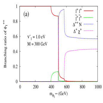
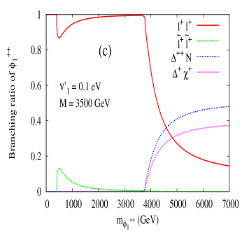
Figure 4: Branching ratios of $\phi^{++}_{1}$ decay modes. In all the decay modes we have summed over the generation index of product particles, see text for details.

While plotting the branching ratios, we have summed over the indices $j,k$. For instance, the branching ratio of $\phi^{++}_{1}$ into same sign charged dileptons is taken as $Br(\phi^{++}_{1}\to\ell^{+}\ell^{+})=\frac{\sum_{j,k=1}^{3}\Gamma(\phi^{++}_{1}\to\ell^{+}_{j}\ell^{+}_{k})}{\Gamma_{\phi^{++}_{1}}}$, where $\Gamma_{\phi^{++}_{1}}$ is the total decay width of $\phi^{++}_{1}$. Similarly, the three charged sleptons, the four neutralinos and the two charginos are summed in the decay modes of $\phi^{++}_{1}\to\tilde{l}^{+}\tilde{l}^{+}$, $\phi^{++}_{1}\to\Delta^{++}_{1}N$ and $\phi^{++}_{1}\to\Delta^{+}_{1}\chi^{+}$, respectively. In the plots of Fig. 4, we can notice that both the dilepton and di-slepton modes will be suppressed as soon as the modes into SUSY fermionic particles are kinematically accessible. The reason for this is as follows. Apart from coupling strengths, in the limit of large mass of $\phi^{++}_{1}$, the decay widths of $\phi^{++}_{1}$ into charged dilepton and into SUSY fermionic particles vary as $\sim m_{\phi^{++}_{1}}$, while the corresponding decay width for $\phi^{++}_{1}$ into charged di-slepton is $\sim\frac{A_{\nu}^{2}}{m_{\phi^{++}_{1}}}$. From the above forms of decay widths, in the limit $m_{\phi^{++}_{1}}\to\infty$, it is clear that the decay mode into charged di-slepton cannot stand against decay modes into dilepton and into SUSY fermionic particles. The decay modes into charged dileptons are driven by Yukawa couplings, which are about $\sim 10^{-3}$ for $v^{\prime}_{1}=$ 1.0 eV. Here the Yukawa couplings are far less than the gauge couplings which drive the decay modes into SUSY fermionic particles, and hence these modes are dominant over the charged dileptons.

In Fig. 4(a) we have chosen $v^{\prime}_{1}=$ 1.0 eV and the mass of fermionic triplet is 300 GeV which satisfies the flavor constraints described in the previous section. For $M=$ 300 GeV, the SUSY modes involving the neutralinos and charginos are kinematically accessible at about $m_{\phi^{++}_{1}}\sim$ 500 and 575 GeV, respectively. As argued in the previous section, the LFV processes have put a lower bound on $m_{\phi^{++}_{1}}$ to be about 630 GeV. Hence, in the case of Fig. 4(a), the scalar field $\phi^{++}_{1}$ can be detected in a collider experiment through its decays into SUSY fermionic particles, because both the charged dilepton and charged di-slepton modes are suppressed for $m_{\phi^{++}_{1}}>$ 630 GeV. However, in Fig. 4(b) we have increased $M$ to 600 GeV so that the SUSY fermionic modes are kinematically accessible at about $m_{\phi^{++}_{1}}\sim$ 800 GeV. Now, in this case, there is an appreciable branching ratio of $\sim$ 90$\%$ to detect $\phi^{++}_{1}$ in the charged dilepton mode for $m_{\phi^{++}_{1}}$ between about 630 to 800 GeV. In the same mass range of $m_{\phi^{++}_{1}}\sim$ 630$-$800 GeV, the probability of detecting $\phi^{++}_{1}$ in the charged di-slepton mode is hardly about 10$\%$. However, by increasing $A_{\nu}$ from 500 GeV to 1 TeV, this probability can be enhanced to 30$\%$, while at the same time the probability into the charged dilepton mode will decrease to about 70$\%$. In Fig. 4(c) we have decreased $v^{\prime}_{1}$ to 0.1 eV and have taken $M=$ 3500 GeV. In this case, there will be enhancement in the Yukawa couplings compared to the previous cases, and the lower limit on $m_{\phi^{++}_{1}}$ from the LFV processes is about 6300 GeV. Because of the enhancement of the Yukawa couplings, the decay mode into charged dilepton is still significant with a branching ratio of $\sim 17\%$ for $m_{\phi^{++}_{1}}>$ 6300 GeV.

We can compare the results of Fig. 4 with that in the non-SUSY version of Type II seesaw model at TeV scale. In the non-SUSY version, only the decay modes into dilepton and di-gauge boson will be present [32]. However, as argued previously, the decay mode into di-gauge boson will be suppressed in our context. The best channel to detect a scalar triplet Higgs is in the decay $\phi^{++}_{1}\to\ell^{+}\ell^{+}$, which has less background in a collider experiment. However, in this model, this channel is restricted by the decay modes into SUSY particles as well as by constraints from the LFV processes. Whereas, in the non-SUSY version of Type II seesaw model, even after imposing the constraints from LFV processes, due to non-existence of decay modes into SUSY particles, we would still have high branching ratio for the decay $\phi^{++}_{1}\to\ell^{+}\ell^{+}$, provided $v^{\prime}_{1}<$ 0.1 MeV [32].

Decay modes of the scalar field $\phi^{+}_{1}$ are as follows: neutrino and charged lepton ($\nu_{j}\ell^{+}_{k}$), anti-sneutrino and charged slepton ($\tilde{\nu}^{*}_{j}\tilde{l}^{+}_{k}$), singly charged fermionic triplet and neutralino ($\Delta^{+}_{1}N_{k}$), doubly charged fermionic triplet and chargino ($\Delta^{++}_{1}\chi^{-}_{k}$), neutral fermionic triplet and chargino ($\Delta^{0}_{1}\chi^{+}_{k}$). The branching ratios of $\phi^{+}_{1}$ as function of its mass are given in Fig. 5, in the case of NH.

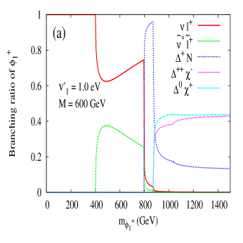
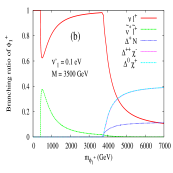
Figure 5: Branching ratios of $\phi^{+}_{1}$ decay modes. In all the decay modes we have summed over the generation index of product particles, see text for details.

As explained around Fig. 4, here also, in the branching ratios of $\phi_{1}^{+}$ into leptons and into supersymmetric particles, we have summed over the indices $j,k$ of the leptons, sleptons, neutralinos and charginos. Like what happened in the case of $\phi^{++}_{1}$ decays, in Fig. 5 we can observe that the decay modes into leptons and into sleptons cannot stand against the modes into SUSY fermionic particles. Unlike in the case of $\phi^{++}_{1}$, the decay $\phi^{+}_{1}\to\nu\ell^{+}$ which is driven by Yukawa couplings is not useful for detecting the scalar triplet, since the neutrino is hard to detect in a collider experiment. Hence for detecting the scalar field $\phi^{+}_{1}$, the modes into SUSY fermionic particles are the best ones. The decay channel into $\tilde{\nu}^{*}\tilde{l}^{+}$ can be used for the detection $\phi_{1}^{+}$ only for a certain choice of parametric values. In Fig. 5(a) where $v^{\prime}_{1}=$ 1.0 eV and $M=$ 600 GeV, the decay mode into $\tilde{\nu}^{*}\tilde{l}^{+}$ can be detected in the experiments with a branching ratio of nearly 30$\%$ for $m_{\phi^{+}_{1}}\sim$ 630$-$800 GeV. However, as explained around Fig. 4, by decreasing $M$ below about 450 GeV and for $v^{\prime}_{1}=$ 1.0 eV, the decay channel into $\tilde{\nu}^{*}\tilde{l}^{+}$ would be suppressed. In Fig. 5(b) we have taken $v^{\prime}_{1}=$ 0.1 eV and $M=$ 3500 GeV. In this plot both the decay modes involving chargino particles give approximately the same branching ratio. By comparing the plots between Figs. 4 and 5, we can notice that for a large value of $m_{\phi_{1}}$, the branching ratio of $\phi_{1}\to\Delta N$ has higher value compared to that of $\phi_{1}\to\Delta\chi$ in Fig. 4, whereas it is vice-versa in Fig. 5. We believe the reason for this is that the coupling of $\phi^{++}_{1}(\phi^{+}_{1})$ to $\Delta^{++}_{1}N_{k}(\Delta^{+}_{1}N_{k})$ is proportional to $gV^{N}_{2k}+g^{\prime}V^{N}_{1k}(g^{\prime}V^{N}_{1k})$. Since $g>g^{\prime}$, that would explain the above mentioned observation.

Decay modes of the scalar field $\phi^{0}_{1}$ are as follows: pair of neutrinos ($\nu_{j}\nu_{k}$), pair of anti-sneutrinos ($\tilde{\nu}^{*}_{j}\tilde{\nu}^{*}_{k}$), neutral fermionic triplet and neutralino ($\Delta^{0}_{1}N_{k}$), singly charged fermionic triplet and chargino ($\Delta^{+}_{1}\chi^{-}_{k}$). The branching ratios of $\phi^{0}_{1}$ as function of its mass are given in Fig. 6, in the case of NH.

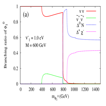
Figure 6: Branching ratios of $\phi^{0}_{1}$ decay modes. In all the decay modes we have summed over the generation index of product particles, see text for details.

Similar to what we have done in Figs. 4 and 5, here also we have summed over the indices $j,k$. As in the case for $\phi_{1}^{+}$, the detection of $\phi^{0}_{1}$ can be mainly found from its decays into SUSY fermionic particles. Also, for some specific choices of $v^{\prime}_{1}$ and $M$, we can use the decay channel into a pair of anti-sneutrinos for the detection of $\phi^{0}_{1}$. In Fig. 6(a), the branching ratio for the decay channel into $\tilde{\nu}^{*}\tilde{\nu}^{*}$ is not larger than 10$\%$ in the allowed region of $m_{\phi^{0}_{1}}\sim$ 630$-$800 GeV. However, this branching ratio can be increased by increasing the value of $A_{\nu}$ from its input value of 500 GeV.

A final comment on the decay branching ratios of $\phi^{+}_{1}$ and $\phi^{0}_{1}$, which are described in Figs. 5 and 6, are as follows. In the littlest Higgs model with SU(5) symmetry [33], both the doublet and triplet scalar states of the gauged SU(2)_L will be put into one single SU(5) multiplet. As a result of this, we can see that the decay branching ratios of $\phi^{+}\to t\bar{b}$ and $\phi^{0}\to t\bar{t}$ are significant [34] in the littlest Higgs model. However, as explained before, in our model, the above mentioned decay processes are suppressed due to small admixture between doublet and triplet scalar fields. Hence, in a collider experiment, the decays of $\phi_{1}^{+}$ and $\phi_{1}^{0}$ can be used to distinguish the Type II seesaw model at TeV scale and the littlest Higgs model.

So far we have dealt with the decays of $\phi_{1}$s and in this model there is another scalar triplet $\phi_{2}$ with a hypercharge of $-1$. As explained before, to simplify the decay channels of scalar triplets, we have chosen $B_{T}=0$. As a result of this, the charged and neutral components of $\phi_{2}$ will dominantly decay into the modes involving SUSY fermionic particles such as fermionic triplet Higgses, neutralinos and charginos. The expressions for the decay widths of these modes are similar to the corresponding $\phi_{1}$ decay modes, Eq. (21). The decay modes of $\phi_{2}$ have no competing channels involving dilepton, and hence the branching ratios of $\phi_{2}$ will be constant in the limit of large masses of these fields.

6 Detection prospects of low energy SUSY Type II seesaw model

As explained in the previous section, one way of probing the low energy Type II seesaw model is to look for signals of scalar triplet Higgs fields in collider experiments. The decay modes of scalar triplet fields which are driven by the Yukawa couplings should be looked at collider experiments in order to verify the neutrino mass mechanism. In this regard, the decay channel $\phi_{1}^{++}\to\ell^{+}\ell^{+}$ is the best mode to probe in experiments. At the LHC, doubly charged scalar triplets can be pair produced through Drell-Yan process. It has been reported in Ref. [30] that the cross section for this pair production is about 1 to 0.1 fb for $m_{\phi^{++}}$ between about 600 to 1000 GeV. In the case of Drell-Yan process, the final signal would be 4 leptons of the form $\ell^{+}\ell^{+}\ell^{-}\ell^{-}$. One can also singly produce $\phi^{\pm\pm}$ at the LHC through the process $q^{\prime}\bar{q}\to W^{*}\to\phi^{\pm\pm}\phi^{\mp}$ [29]. It has been claimed in Ref. [29] that the cross section for the single production of $\phi^{\pm\pm}$ can be enhanced by about a factor of 2 compared to the Drell-Yan case. In the case of single production of $\phi^{\pm\pm}$, the final signal would be 3 leptons of the form $\ell^{\pm}\ell^{\pm}\ell^{\mp}$. In the previous section, we have described that the decay modes of scalar triplets into leptons will compete with decay modes into supersymmetric particles. In Figs. 4(b) and 5(a), $\phi^{++}_{1}\to\ell^{+}\ell^{+}$ and $\phi^{+}_{1}\to\ell^{+}\nu$ have appreciable branching ratios of $\sim$0.9 and $\sim$0.7, respectively, for $m_{\phi^{++}_{1}}$ between 630 to 800 GeV. Assuming an integrated luminosity of 100 fb^-1 at the LHC in future, we can observe about 8 to 80 events for $m_{\phi^{++}_{1}}$ between 630 to 800 GeV, in the case of 4-lepton signal. In the case of 3-lepton signal, about 12 to 120 events can be observed at the LHC. However, these event numbers are calculated without including background processes and simulation cuts, and a detailed analysis should be done in order to detect the scalar triplet fields at the LHC. Apart from the above described 4-lepton and 3-lepton signals, there can be other possibilities in our model. In either of the processes $q\bar{q}(\bar{q}^{\prime})\to\phi^{++}\phi^{--}(\phi^{-})$, one doubly charged scalar triplet can decay into dilepton, whereas, the other scalar triplet can decay into SUSY particles. In these processes, there can be flavor violating decays $\phi^{--}\to e\mu,\mu\tau$, etc at the LHC.

We comment on the detection prospects of our model compared to the Type II seesaw models where the triplet fields are super heavy. As already described before, in our model the triplet fields have masses around 1 TeV and we have assumed that off-diagonal entries in the soft masses of sleptons are zero. However, in models where triplet fields are super heavy, due to renormalization effects, slepton mass matrix can acquire non-zero off-diagonal elements. In fact, in this class of models [9, 10], it has been shown that various LFV processes are correlated by the same model parameters, and flavor violating decays of staus and neutralinos can be observed at the LHC [10]. In our model these processes are absent, however, LFV decays of charged triplet fields of this model can be observed at the LHC. We have commented on one such possibility in the previous paragraph.

In our model the flavor violation is driven by the off-diagonal elements of Yukawa couplings, $Y_{\nu}$. Hence, flavor violation in our model can be probed at LHC in the decay modes of $\phi_{1}^{++}$ into charged leptons, which are presented in Fig. 4. Since the Yukawa couplings in different hierarchical patterns of neutrinos would be different, $BR(\phi_{1}^{++}\to\ell\ell)$ would be different in these different cases, which should offer different signal strength at the LHC. Moreover, as described before, the elements of $Y_{\nu}$ are nearly $\sim 10^{-3}$ for $v^{\prime}_{1}$ = 1 eV in the cases of NH and IH. Whereas, in the case of DN, the diagonal and off-diagonal elements of $Y_{\nu}$ are $\sim$0.1 and $\sim 10^{-4}$, respectively, for $v^{\prime}_{1}$ = 1 eV. The difference in Yukawa couplings give different values for, say $BR(\phi_{1}^{++}\to e^{+}e^{+})$ and $BR(\phi_{1}^{++}\to e^{+}\mu^{+})$, which should be probed at LHC to distinguish the case of DN from NH and IH.

Apart from accelerator based experiments, neutrinoless double beta decay ($0\nu\beta\beta$) experiments offer alternative probes for new physics models where neutrinos are Majorana particles. In the Type II seesaw model at TeV scale, the scalar triplet Higgses, through a sub-process $W^{-}W^{-}\to\phi^{--}\to\ell^{-}\ell^{-}$, can give additional contribution to $0\nu\beta\beta$ [35]. But due to small couplings and heavy masses of these fields, this additional contribution is highly negligible, and hence the amplitude for $0\nu\beta\beta$ is dominantly contributed by the Majorana neutrinos [35].

7 Conclusions

In this work we have focused on the phenomenological implications of supersymmetric Type II seesaw model at TeV scale. In this model, there are two triplet superfields with hypercharges $Y=+1,-1$, whose scalar and fermionic components will have masses at around TeV scale. Also, the smallness of neutrino masses can be naturally explained in this model, provided the vevs of the neutral scalar triplet fields are around 1 eV. In this scenario, the Yukawa couplings of the triplet field ($Y=+1$) to the lepton doublets are unsuppressed and these couplings can drive LFV processes. We have focused on a particular parameter space of the model where the loop induced processes due to charged slepton and sneutrino fields give negligible contribution to the LFV processes. Another simplified assumption we have made is that we have neglected the mixing between scalar components of the two different triplet superfields.

After making the above assumptions, the branching ratios of LFV processes in the Type II seesaw model depend dominantly on the Yukawa couplings and masses of the triplet fields. The Yukawa couplings in this model are determined by the neutrino oscillation data and the scalar triplet vev $v_{1}^{\prime}$. Specifically, we have found that among the various possible LFV processes, the current experimental upper limits on the branching ratios of $\mu\to 3e$ and $\mu\to e\gamma$ can put lower limits on the masses of triplet Higgs states. The masses of scalar ($m_{\phi}$) and fermionic ($M$) triplet Higgs states should be at least 630 and 200 GeV, respectively. We have tabulated the lower limits on the masses of these fields in Tabs. 1 and 2. The lower limits on $m_{\phi}$ and $M$ depend on the hierarchical mass pattern of neutrinos and also on $v_{1}^{\prime}$. The bounds on $M$ also depend on the masses of sleptons. For slepton masses as low as 200 GeV we get stringent bounds on $M$, which are displayed in Tab. 2.

Next, we have addressed the implications of the constraints from LFV processes on observable quantities such as the muon anomalous magnetic moment, $(g-2)_{\mu}$. In the case of degenerate mass pattern of neutrinos, the contribution to the $(g-2)_{\mu}$ from the scalar and fermionic triplet Higgses can fit the current discrepancy in it. However, after applying the constraints from the above described LFV processes, this contribution will be at most $3.4\times 10^{-11}$, which is two orders less than the required amount.

We have also studied the detection of scalar triplet fields in a collider experiment, and for this we have studied decay patterns of these fields. While studying these decay processes, we have applied the same assumptions which we have applied in our study on the LFV processes, which are described above. As a result of this, the scalar triplet fields ($\phi_{1}$s) which have hypercharge $Y=+1$ can decay into leptonic as well as supersymmetric particles. Whereas, the scalar triplet fields which have hypercharge $Y=-1$ can decay only into supersymmetric fields. The golden channel to detect any of these scalar triplet Higgses is $\phi^{++}_{1}\to\ell^{+}\ell^{+}$, and we have addressed how this channel will be affected due to the presence of decay modes involving supersymmetric particles. Our study suggests that the above mentioned golden channel may not compete against the decay modes into supersymmetric particles. However, for some suitable choice of model parameters, where $M$ = 600 GeV and for $m_{\phi}$ between about 630 to 800 GeV, $BR(\phi^{++}_{1}\to\ell^{+}\ell^{+})$ can be as high as 90$\%$. Similarly, after applying the constraints from LFV and depending on the choice of parameter space, the singly charged ($\phi^{+}_{1}$) and neutral ($\phi^{0}_{1}$) scalar triplet Higgses can be detected in the modes involving supersymmetric fields.

Flavor violation in our model can take place through decays such as $\phi^{--}\to e\mu,\mu\tau,$ etc. Probing such flavor violation in the LHC can not only test the Type II seesaw mechanism of our model but also can be used to distinguish different hierarchical mass patterns of neutrinos.

Appendix

A) Scalar potential

The scalar potential of the SUSY Type II seesaw model at TeV scale will have the following form.

$$V = \sum_{Y}\left|\frac{\partial W}{\partial Y}\right|^{2}+\frac{1}{2}\sum_{a=1}^{3}D^{a}D^{a}+\frac{1}{2}D^{Y}D^{Y}+V_{\rm soft}^{\rm MSSM}+V_{\rm soft}^{\rm triplet},$$ (23)

$$D^{a} = -g\left(H_{d}^{\dagger}\frac{\sigma^{a}}{2}H_{d}+H_{u}^{\dagger}\frac{\sigma^{a}}{2}H_{u}+\Phi_{1}^{\dagger}T^{a}\Phi_{1}+\Phi_{2}^{\dagger}T^{a}\Phi_{2}\right),$$

$$D^{Y} = -\frac{g^{\prime}}{2}\left(H^{\dagger}_{u}H_{u}-H^{\dagger}_{d}H_{d}\right)-g^{\prime}\left(\Phi_{1}^{\dagger}\Phi_{1}-\Phi^{\dagger}_{2}\Phi_{2}\right).$$

The first term in Eq. (23) is the $F$-term contribution where the summation over the fields $Y$ run over the superfields of $W$ of Eq. (1). The second and third terms of Eq. (23) are $D$-term contributions due to SU(2)_L and U(1)_Y gauge groups, respectively. The last two terms of Eq. (23) are soft terms of MSSM and of fields involving triplet scalar fields. The form of $V_{\rm soft}^{\rm MSSM}$ can be found in Ref. [6, 7]. The $V_{\rm soft}^{\rm triplet}$ is given in Eq. (5). The triplet representation of SU(2) generators, which are needed in $D^{a}$ of Eq. (23), are

$$T^{1}=\frac{1}{\sqrt{2}}\left(\begin{array}[]{ccc}0&1&0\\ 1&0&1\\ 0&1&0\end{array}\right),\quad T^{2}=\frac{1}{\sqrt{2}}\left(\begin{array}[]{ccc}0&-i&0\\ i&0&-i\\ 0&i&0\end{array}\right),\quad T^{3}=\left(\begin{array}[]{ccc}1&0&0\\ 0&0&0\\ 0&0&-1\end{array}\right).$$ (24)

For computing $D$-terms, the forms of the scalar fields are as follows: $H_{u}=(H^{+}_{u},H^{0}_{u})^{\rm T}$, $H_{d}=(H^{0}_{d},H^{-}_{d})^{\rm T}$, $\Phi_{1}=(\phi_{1}^{++},\phi^{+}_{1},\phi^{0}_{1})^{\rm T}$, $\Phi_{2}=(\phi_{2}^{0},\phi^{-}_{2},\phi^{--}_{2})^{\rm T}$. We have described the $D$-terms of doublet and of triplet Higgses, but the $D$-terms for other scalar fields of the model can be analogously written.

B) Conventions of neutralino and chargino mass matrices and their diagonalizing matrices

Our conventions regarding neutralino and chargino mass matrices are same as in [7]. In the basis $\Psi^{0}=(\tilde{B},\tilde{W}^{3},\tilde{H}_{d},\tilde{H}_{u})^{\rm T}$, the mixing mass matrix of neutralinos can be written as ${\cal L}_{N}=-\frac{1}{2}\left(\Psi^{0}\right)^{\rm T}M_{N}\Psi^{0}+{\rm h.c.}$. The form of $M_{N}$ is same as Eq. (8.2.2) of Ref. [7]. The physical neutralino states are defined from $\Psi^{0}_{j}=\sum_{k=1}^{4}V^{N}_{jk}N_{k}$, where the unitary matrix $V^{N}$ diagonalizes $M_{N}$ as

$$\left(V^{N}\right)^{\rm T}M_{N}V^{N}={\rm diag}(m_{N1},m_{N2},m_{N3},m_{N4}).$$ (25)

In the basis: $\Psi^{-}=(\tilde{W}^{-},\tilde{H}^{-}_{d})^{\rm T}$, $\Psi^{+}=(\tilde{W}^{+},\tilde{H}^{+}_{u})^{\rm T}$, the mixing mass terms for charginos can be written as ${\cal L}_{c}=-\left(\Psi^{-}\right)^{\rm T}M_{C}\Psi^{+}+{\rm h.c.}$. The matrix $M_{C}$ is same as Eq. (8.2.14) of Ref. [7]. The physical chargino states are defined from: $\Psi^{-}_{j}=\sum_{k=1}^{2}U^{\chi}_{jk}~{}\chi^{-}_{k}$, $\Psi^{+}_{j}=\sum_{k=1}^{2}V^{\chi}_{jk}~{}\chi^{+}_{k}$. The unitary matrices $U^{\chi}$ and $V^{\chi}$ diagonalize $M_{C}$ as

$$\left(U^{\chi}\right)^{\rm T}M_{C}V^{\chi}={\rm diag}(m_{C1},m_{C2}).$$ (26)

References

- [1] G. Aad et al. [ATLAS Collaboration], Phys. Lett. B 716, 1 (2012) [arXiv:1207.7214 [hep-ex]]; S. Chatrchyan et al. [CMS Collaboration], Phys. Lett. B 716, 30 (2012) [arXiv:1207.7235 [hep-ex]].
- [2] M. E. Peskin, In *Carry-le-Rouet 1996, High-energy physics* 49-142 [hep-ph/9705479]; G. Altarelli, Nucl. Instrum. Meth. A 518, 1 (2004) [hep-ph/0306055]; C. Quigg, hep-ph/0404228; J. Ellis, Nucl. Phys. A 827, 187C (2009) [arXiv:0902.0357 [hep-ph]].
- [3] T. Mori, eConf C 060409, 034 (2006) [hep-ex/0605116]; J. M. Yang, Int. J. Mod. Phys. A 23, 3343 (2008) [arXiv:0801.0210 [hep-ph]]; A. J. Buras, Acta Phys. Polon. Supp. 3, 7 (2010) [arXiv:0910.1481 [hep-ph]]; Y. Nir, CERN Yellow Report CERN-2010-001, 279-314 [arXiv:1010.2666 [hep-ph]].
- [4] For a review on neutrino masses and mixing, see R. N. Mohapatra, hep-ph/0211252; Y. Grossman, hep-ph/0305245; A. Strumia and F. Vissani, hep-ph/0606054.
- [5] M. Magg and C. Wetterich, Phys. Lett. B 94, 61 (1980); J. Schechter and J. W. F. Valle, Phys. Rev. D 22, 2227 (1980); R. N. Mohapatra and G. Senjanovic, Phys. Rev. D23, 165 (1981); G. Lazarides, Q. Shafi and C. Wetterich, Nucl. Phys. B 181, 287 (1981).
- [6] H. P. Nilles, Phys. Rept. 110, 1 (1984); H. E. Haber and G. L. Kane, Phys. Rept. 117, 75 (1985); M. Drees, R. Godbole and P. Roy, Theory and Phenomenology of Sparticles, (World Scientific, 2004); P. Binetruy, Supersymmetry (Oxford University Press, 2006); H. Baer and X. Tata, Weak Scale Supersymmetry: From Superfields to Scattering Events, (Cambridge University Press, 2006).
- [7] S. P. Martin, arXiv:hep-ph/9709356.
- [8] T. Hambye, E. Ma and U. Sarkar, Nucl. Phys. B 602, 23 (2001) [hep-ph/0011192].
- [9] A. Rossi, Phys. Rev. D 66, 075003 (2002) [hep-ph/0207006].
- [10] M. Hirsch, S. Kaneko and W. Porod, Phys. Rev. D 78, 093004 (2008) [arXiv:0806.3361 [hep-ph]]; J. N. Esteves, J. C. Romao, A. Villanova del Moral, M. Hirsch, J. W. F. Valle and W. Porod, JHEP 0905, 003 (2009) [arXiv:0903.1408 [hep-ph]].
- [11] S. Antusch and S. F. King, Phys. Lett. B 597, 199 (2004) [hep-ph/0405093]; E. J. Chun and S. Scopel, Phys. Lett. B 636, 278 (2006) [hep-ph/0510170]; M. Senami and K. Yamamoto, Int. J. Mod. Phys. A 21, 1291 (2006) [hep-ph/0305202].
- [12] A. G. Akeroyd and S. Moretti, Phys. Rev. D 86, 035015 (2012) [arXiv:1206.0535 [hep-ph]].
- [13] J. Beringer et al. (Particle Data Group), Phys. Rev. D 86, 010001 (2012).
- [14] E. J. Chun, K. Y. Lee and S. C. Park, Phys. Lett. B 566, 142 (2003) [hep-ph/0304069]; M. Kakizaki, Y. Ogura and F. Shima, Phys. Lett. B 566, 210 (2003) [hep-ph/0304254]; E. K. .Akhmedov and W. Rodejohann, JHEP 0806, 106 (2008) [arXiv:0803.2417 [hep-ph]]; W. Rodejohann, Pramana 72, 217 (2009) [arXiv:0804.3925 [hep-ph]].
- [15] A. G. Akeroyd, M. Aoki and H. Sugiyama, Phys. Rev. D 79, 113010 (2009) [arXiv:0904.3640 [hep-ph]].
- [16] T. Fukuyama, H. Sugiyama and K. Tsumura, JHEP 1003, 044 (2010) [arXiv:0909.4943 [hep-ph]].
- [17] M. Senami and K. Yamamoto, Phys. Rev. D 69, 035004 (2004) [hep-ph/0305203].
- [18] For a review on the muon , see, Z. Zhang, arXiv:0801.4905 [hep-ph]; F. Jegerlehner and A. Nyffeler, Phys. Rept. 477, 1 (2009) [arXiv:0902.3360 [hep-ph]].
- [19] R. S. Hundi, S. Pakvasa and X. Tata, Phys. Rev. D 79, 095011 (2009) [arXiv:0903.1631 [hep-ph]].
- [20] J. Adam et al. [MEG Collaboration], Phys. Rev. Lett. 107, 171801 (2011) [arXiv:1107.5547 [hep-ex]].
- [21] J. Chakrabortty, P. Ghosh and W. Rodejohann, arXiv:1204.1000 [hep-ph].
- [22] Y. Abe et al. [DOUBLE-CHOOZ Collaboration], Phys. Rev. Lett. 108, 131801 (2012) [arXiv:1112.6353 [hep-ex]]; F. P. An et al. [DAYA-BAY Collaboration], Phys. Rev. Lett. 108, 171803 (2012) [arXiv:1203.1669 [hep-ex]]; J. K. Ahn et al. [RENO Collaboration], Phys. Rev. Lett. 108, 191802 (2012) [arXiv:1204.0626 [hep-ex]].
- [23] D. V. Forero, M. Tortola and J. W. F. Valle, arXiv:1205.4018 [hep-ph].
- [24] P. F. Harrison, D. H. Perkins and W. G. Scott, Phys. Lett. B 530, 167 (2002) [hep-ph/0202074].
- [25] S. Chatrchyan et al. [CMS Collaboration], arXiv:1207.2666 [hep-ex].
- [26] T. Moroi, Phys. Rev. D 53, 6565 (1996) [Erratum-ibid. D 56, 4424 (1997)] [hep-ph/9512396]; S. P. Martin and J. D. Wells, Phys. Rev. D 64, 035003 (2001) [hep-ph/0103067].
- [27] R. S. Hundi, Phys. Rev. D 83, 115019 (2011) [arXiv:1101.2810 [hep-ph]].
- [28] J. F. Gunion, R. Vega and J. Wudka, Phys. Rev. D 42, 1673 (1990); R. Godbole, B. Mukhopadhyaya and M. Nowakowski, Phys. Lett. B 352, 388 (1995) [hep-ph/9411324]; K. -m. Cheung, R. J. N. Phillips and A. Pilaftsis, Phys. Rev. D 51, 4731 (1995) [hep-ph/9411333]; M. Muhlleitner and M. Spira, Phys. Rev. D 68, 117701 (2003) [hep-ph/0305288]; E. J. Chun and P. Sharma, JHEP 1208, 162 (2012) [arXiv:1206.6278 [hep-ph]].
- [29] A. G. Akeroyd and M. Aoki, Phys. Rev. D 72, 035011 (2005) [hep-ph/0506176].
- [30] T. Han, B. Mukhopadhyaya, Z. Si and K. Wang, Phys. Rev. D 76, 075013 (2007) [arXiv:0706.0441 [hep-ph]].
- [31] D. A. Demir, M. Frank, D. K. Ghosh, K. Huitu, S. K. Rai and I. Turan, Phys. Rev. D 79, 095006 (2009) [arXiv:0903.3955 [hep-ph]].
- [32] A. G. Akeroyd and H. Sugiyama, Phys. Rev. D 84, 035010 (2011) [arXiv:1105.2209 [hep-ph]].
- [33] N. Arkani-Hamed, A. G. Cohen, E. Katz and A. E. Nelson, JHEP 0207, 034 (2002) [hep-ph/0206021].
- [34] T. Han, H. E. Logan, B. Mukhopadhyaya and R. Srikanth, Phys. Rev. D 72, 053007 (2005) [hep-ph/0505260].
- [35] W. Rodejohann, Int. J. Mod. Phys. E 20, 1833 (2011) [arXiv:1106.1334 [hep-ph]].