Clustering, Bias and the Accretion Mode of X-ray selected AGN

Abstract

We present the spatial clustering properties of 1466 X-ray selected AGN compiled from the Chandra CDF-N, CDF-S, eCDF-S, COSMOS and AEGIS fields in the $0.5-8$ keV band. The X-ray sources span the redshift interval $0<z<3$ and have a median value of $\bar{z}=0.976$. We employ the projected two-point correlation function to infer the spatial clustering and find a clustering length of $r_{0}=7.2\pm 0.6h^{-1}$ Mpc and a slope of $\gamma=1.48\pm 0.12$, which corresponds to a bias of $b(\bar{z})=2.26\pm 0.16$. Using two different halo bias models, we consistently estimate an average dark-matter host halo mass of $M_{\rm h}\simeq 1.3(\pm 0.3)\times 10^{13}h^{-1}M_{\odot}$. The X-ray AGN bias and the corresponding dark-matter host halo mass, are significantly higher than the corresponding values of optically selected AGN (at the same redshifts). The redshift evolution of the X-ray selected AGN bias indicates, in agreement with other recent studies, that a unique dark-matter halo mass does not fit well the bias at all the different redshifts probed. Furthermore, we investigate if there is a dependence of the clustering strength on X-ray luminosity. To this end we consider only 650 sources around $z\sim 1$ and we apply a procedure to disentangle the dependence of clustering on redshift. We find indications for a positive dependence of the clustering length on X-ray luminosity, in the sense that the more luminous sources have a larger clustering length and hence a higher dark-matter halo mass. In detail we find for an average luminosity difference of $\delta\log_{10}L_{x}\simeq 1$ a halo mass difference of a factor of $\sim$3.

These findings appear to be consistent with a galaxy-formation model where the gas accreted onto the supermassive black hole in intermediate luminosity AGN comes mostly from the hot-halo atmosphere around the host galaxy.

1 Introduction

One of the most remarkable astonomical findings of the last decade is the discovery of the scaling relations between the mass of supermassive black holes (BHs) and the properties of the large-scale environment of their host galaxies. In particular, observations suggest that there is a tight correlation between the BH mass and the bulge velocity dispersion, stellar mass and luminosity of the spheroidal component of the host galaxy (e.g., Ferrarese & Ford, 2005; Magorrian et al., 1998), Häring & Rix (2004); Gültekin et al. (2009). These observational relations indicate that the cosmic growth of BH mass is strongly coupled to the evolution of the host spheroid. However, the physical mechanism that shapes these relations is still unknown.

In most semi-analytic models of galaxy formation (e.g., Croton et al., 2006; Bower et al., 2006; Lagos et al., 2008), Somerville et al. (2008) it is assumed that the active galactic nucleus (AGN) associated with accreting black hole regulates the formation of new stars. The mechanisms adopted by semi-analytical models for triggering AGN activity include major galaxy mergers for the most luminous AGN (Di Matteo et al., 2005; Hopkins et al., 2006; Marulli et al., 2009), while it is possible that in the lowest luminosity AGN regime secular disk instabilities or minor interactions play the key role (Hopkins & Hernquist, 2006; Bournaud et al., 2011). These different AGN fueling modes make diverse predictions for the environment of the galaxies that host AGN (Shankar et al., 2009). For example, in the major-merger scenario, only weak luminosity dependence on clustering is expected (Hopkins et al., 2005; Lidz et al., 2006; Bonoli et al., 2009). Hence, observational studies of AGN clustering and its dependence on luminosity can place valuable constraints on the AGN fueling modes and consequently on the AGN–galaxy co-evolution models.

The clustering of AGN has been studied with excellent statistics mainly in the optical and particularly in large area surveys, such as the 2QZ (2dF QSO Redshift Survey Croom et al., 2005; Porciani & Norberg, 2006) and the SDSS (Sloan Digital Sky Survey, Li et al., 2006; Shen et al., 2009; Ross et al., 2009). These surveys found no evidence for a strong dependence of clustering on luminosity (e.g., Croom et al., 2005; Myers et al., 2006; da Ângela et al., 2008) although Shen et al. (2009) detect an excess of clustering for their 10% brightest quasars. However, optical QSO may represent only the tip of the iceberg of the AGN population. Very deep X-ray surveys find a surface density of about 10,000 deg^-2 (Xue et al., 2011), which is about two orders of magnitude higher than that found in optical QSO surveys (Wolf et al., 2003). Several studies have explored the angular clustering of AGN in X-ray wavelengths (Vikhlinin & Forman, 1995; Akylas et al., 2000; Yang et al., 2003), (Basilakos et al., 2004, 2005), Gandhi et al. (2006), Puccetti et al. (2006), Carrera et al. (2007), Miyaji et al. (2007), Plionis et al. (2008), Ebrero et al. (2009), Elyiv et al. (2012). These studies measure the projected angular clustering and then via Limber’s equation (Peebles, 1980) derive the corresponding spatial clustering length. However, in this method an a priori knowledge of the redshift distribution $dN/dz$ is needed and thus, the uncertainties may be appreciable. Plionis et al. (2008) first reported strong indications for a luminosity dependent clustering of X-ray AGN in the CDF fields for both soft and hard bands in the sense that X-ray luminous AGN lie in more massive dark-matter (DM) halos compared to the less luminous ones.

Recently, several studies have attempted to measure the spatial correlation function of X-ray selected AGN by employing spectroscopic redshifts to estimate their correct distances (Mullis et al., 2004; Gilli et al., 2005; Yang et al., 2006), (Gilli et al., 2009; Hickox et al., 2009; Coil et al., 2009), Krumpe et al. (2010), (Cappelluti et al., 2010; Miyaji et al., 2011), (Starikova et al., 2011; Allevato et al., 2011). These studies show that X-ray AGN are typically hosted in DM halos with mass of the order of $12.5<\log_{10}(M_{\rm h}/[h^{-1}M_{\odot}])<13.5$, at a redshift $z\sim 1$. On the issue of luminosity dependent clustering the results are contentious. Yang et al. (2006) did not detect strong correlation between X-ray luminosity and the clustering amplitude for Chandra sources. Gilli et al. (2009) performed a similar investigation in the XMM-COSMOS field dividing the sample below and above $L_{x}(0.5-10{\rm keV})=10^{44}~{}\rm{erg~{}s}^{-1}$ and did not find any luminosity dependence. Similarly, Starikova et al. (2011), using 1282 Chandra/Bootes sources, did not find a significant dependence of clustering on luminosity.

On the other hand, Coil et al. (2009) using AGN in the redshift range $z=0.7-1.4$ from the AEGIS field found a weak evidence for a luminosity dependent clustering, but not at a statistically significant level. In addition, Krumpe et al. (2010) using low redshift ($z\sim 0.25$) AGN, selected from the ROSAT all-sky survey and cross matched with the SDSS, found that $L_{x}>10^{44}~{}\rm{erg~{}s}^{-1}$ sources are clustered more strongly than lower luminosity sources. In another recent study, Cappelluti et al. (2010) using a sample of 199 Swift-BAT sources in the $15-55~{}\rm{keV}$ band, found a marginally significant luminosity dependent clustering.

In this paper we use a sample of $1466$ sources selected in the $0.5-8~{}\rm{keV}$ band from a variety of deep Chandra X-ray surveys, to estimate the spatial correlation function and typical DM host halo mass of X-ray selected AGN. Our aim is to investigate whether there is a luminosity dependence on clustering, but also to obtain insight into the black-hole fueling mechanisms, using the largest X-ray selected AGN sample used so far for this scope. The paper is organized as follows. In Section 2, we briefly discuss the X-ray surveys we consider in this paper and in Section 3, we describe the methodology of our clustering analysis. In Section 4, we present our findings for the AGN correlation function as estimated by the joint and individual X-ray samples. In Section 5, we calculate the bias of AGN and its redshift evolution, and estimate the average mass of the DM halos hosting X-ray AGN. In Section 6, we investigate the dependence of the halo mass on X-ray luminosity and compare our findings with theoretical galaxy formation models for the evolution of accreting BHs. Finally, we present in Section 7 our conclusions. For comparison reasons with previous works we adopt, unless otherwise stated, a flat cosmology with a present-day matter density parameter $\Omega_{m}=0.3$, a cosmological constant $\Omega_{\rm{\Lambda}}=0.7$ and baryon density $\Omega_{b}=0.04$. The Hubble constant is expressed in units of $h$ as $H_{0}=100~{}h$ km s^-1 Mpc ^-1.

2 AGN CATALOGS

We make use of X-ray data coming from the five deepest X-ray surveys, namely the Chandra Deep Field South and North (CDF-S and CDF-N), the AEGIS, the extended Chandra Deep Field South (ECDF-S) and the COSMOS survey. These cover a variety of exposures (from $4~{}\rm{Ms}$ down to $40~{}\rm{ksec}$) and surveyed area and thus, cover extensively the luminosity-redshift space. Moreover, these fields contain excellent quality spectroscopic observations and therefore good quality redshifts, which are essential in this project. Below we present briefly the main characteristics of the X-ray surveys used in this work.

2.1 CHANDRA DEEP FIELD NORTH

The deep pencil beam CDF-N survey covers an area of $448~{}\rm{arcmin}^{2}$, is centered at $a=12^{h}36^{m}49^{s},\delta=+62^{\circ}12^{,}58^{,,}$ and consists of 20 individual ACIS-I (Advanced CCD Imaging Spectrometer) pointings. The combined observations provide the deepest X-ray sample currently available together with the CDF-S. Here, we use the X-ray $2~{}\rm{Ms}$ source catalogue of Alexander et al. (2003), with a sensitivity of $\sim 10^{-17}$ erg cm^-2 s^-1, which consists of 503 sources in the $0.5-8$ keV band. Spectroscopic redshifts were used for 243 X-ray sources in the redshift interval $z=0-3$ from Trouille et al. (2008, and references therein).

2.2 CHANDRA DEEP FIELD SOUTH

The deep pencil beam CDF-S survey covers an area of 436 arcmin² and the average aim point is $\rm{a=03^{h}32^{m}28^{s}8,\delta=-27^{\circ}48^{,}23^{,,}(J2000)}$. The analysis of all 23 observations is presented in (Luo et al., 2008). We use the 2Ms X-ray source catalogue of Luo et al. (2008), which consists of 462 X-ray sources. Spectroscopic redshifts were used for 219 X-ray sources in the redshift interval $z=0-3$ from Luo et al. (2010).

2.3 AEGIS

The ultra deep field survey comprises of pointings at 8 separate positions, each with nominal exposure of $200$ ks, covering a total area of approximately $0.67~{}\rm{deg}^{2}$ centered at $a=14^{h}17^{m},\delta=+52^{\circ}30^{,}$ in a strip of length $2~{}\rm{deg}$. The flux limit of the survey is $S\sim 10^{-16}$ erg s^-1cm^-2 in the full band. We use the X-ray source catalogue of Laird et al. (2009), which consists of 1325 sources. Spectroscopic redshifts were used for 392 X-ray sources in the redshift interval $z=0-3$ from DEEP2 (Davis et al., 2001, 2003; Coil et al., 2009).

2.4 COSMOS

The Chandra COSMOS Survey covers the central $0.5~{}\rm{deg}^{2}$ area of the COSMOS field with an effective exposure of $\thicksim 160\rm{ks}$ and the rest of the field with an effective exposure of $\thicksim 80\rm{ks}$. The limiting source detection depths are $5.7\times 10^{-16}$ erg s^-1 cm^-2 in the full band. We use the source catalog of Elvis et al. (2009), which consists of 1761 sources. Spectroscopic redshifts were used for 417 X-ray sources from Brusa et al. (2010).

2.5 EXTENDED CHANDRA DEEP FIELD SOUTH

The ECDF-S survey consists of 4 Chandra $250~{}\rm{ks}$ ACIS-I pointings covering $\sim 0.3$ deg² and surrounding the original CDF-S. Source detection has been performed by Lehmer et al. (2005) and Virani et al. (2006). Here we use the source detection of Lehmer et al. (2005) in which $762$ sources have been detected. The flux limit of ECDF-S is $S\sim 10^{-16}$ erg s^-1cm^-2. Spectroscopic redshifts were used for $288$ sources in the redshift interval $z=0-3$ from Silverman et al. (2010). When combining all fields, we exclude sources that are detected both in ECDF-S and CDF-S and keep only those detected in the ECDF-S.

3 METHODOLOGY

3.1 Theoretical Considerations

The main statistic used to measure the clustering of extragalactic sources is the two-point correlation function $\xi(r)$. $\xi(r)$ describes the excess probability over random of finding a pair with one object in an elemental volume $dV_{1}$ and the second in the elemental volume $dV_{2}$, separated by a distance $r$ (e.g., Peebles, 1980). Its mathematical description is given by $dP=\langle n\rangle^{2}[1+\xi(s)]dV_{1}dV_{2}$, where $\langle n\rangle$ is the mean space density of the sources under study and $s=cz$. When measuring $\xi$ directly from redshift catalogues of sources, we include the distorting effect of peculiar velocities, since the true distance of a source is $r=(s-{\bf v}_{p}\cdot{\bf r})/H_{0}$, where ${\bf v}_{p}\cdot{\bf r}$ is the component of the peculiar velocity of the source along the line of sight. In order to avoid such effects one can either measure the angular clustering, which is not hampered by the effects of $z$-distortions, and then, under some assumptions, infer the spatial correlation function through the Limber’s integral equation (Limber, 1953). Alternatively one can use the redshift information to measure the so-called projected correlation function, $w_{p}(r_{p})$ (e.g., Davis & Peebles, 1983) and then infer the spatial clustering.

To this end, one deconvolves the redshift-based distance of a source, $s$, in two components, one parallel ($\pi$) and one perpendicular ($r_{p}$) to the line of sight, i.e., $s=(r_{p}^{2}+\pi^{2})^{1/2}$, and thus the redshift-space correlation function can be written as $\xi(s)=\xi(r_{p},\pi)$. Since redshift space distortions affect only the $\pi$ component, one can estimate the free of $z$-space distortions projected correlation function, $w_{p}(r_{p})$, by integrating $\xi(r_{p},\pi)$ along $\pi$:

$$w_{p}(r_{p})=2\int_{0}^{\infty}\xi(r_{p},\pi)\mathrm{d}\pi.$$ (1)

Once we estimate the projected correlation function, $w_{p}(r_{p})$, we can recover the real space correlation function, since the two are related according to (Davis & Peebles, 1983)

$$w_{p}(r_{p})=2\int_{0}^{\infty}\xi(\sqrt{r_{p}^{2}+\pi^{2}}){\rm d}\pi=2\int_{r_{p}}^{\infty}\frac{r\xi(r)\mathrm{d}r}{\sqrt{r^{2}-r_{p}^{2}}}\;.$$ (2)

Modelling $\xi(r)$ as a power law, $\xi(r)=\left(r/r_{0}\right)^{-\gamma}$ one obtains,

$$w_{p}(r_{p})=A_{\gamma}r_{p}\left(\frac{r_{0}}{r_{p}}\right)^{\gamma},$$ (3)

with

$$A\gamma=\Gamma\left(\frac{1}{2}\right)\Gamma\left(\frac{\gamma-1}{2}\right)/\Gamma\left(\frac{\gamma}{2}\right),$$ (4)

where $\Gamma$ is the usual gamma function.

However, it should be noted that although Eq. (3) strictly holds for $\pi_{\rm max}=\infty$, practically we always impose a cutoff $\pi_{\rm max}$ (for reasons discussed in the next subsection). This introduces an underestimation of the underlying correlation function, which is an increasing function of separation $r_{p}$. For a power law correlation function this underestimation is easily inferred from Eq. (2) and is given by (e.g., Starikova et al., 2011)

$$C_{\gamma}(r_{p})=\frac{\int_{0}^{\pi_{\rm max}}(r^{2}-\pi^{2})^{-\gamma/2}d\pi}{\int_{0}^{\infty}(r^{2}-\pi^{2})^{-\gamma/2}d\pi}\;.$$ (5)

Thus, by taking into account the above statistical correction, and under the assumption of the power-law correlation function, one can recover the corrected spatial correlation function, $\xi(r_{p})$, from the fit to the measured $w_{p}(r_{p})$ according to (which provides also the value of $\gamma$):

$$\xi(r_{p})=\frac{1}{A_{\gamma}C_{\gamma}(r_{p})}\frac{w_{p}(r_{p})}{r_{p}}\;.$$ (6)

However, at large separations the correction factor increasingly dominates over the signal and thus it constitutes the correction procedure unreliable. Alternatively, as can be easily shown using Eqs. (3) and (6), a crude estimate of the corrected spatial correlation length can be provided by:

$$r_{o,c}=r_{0}C_{\gamma}(r_{0})^{-1/\gamma}\;,$$ (7)

where $r_{0}$ and $\gamma$ are derived from fitting the data to Eq. (3).

3.2 Correlation Function Estimator

As a first step we calculate $\xi(r_{p},\pi)$ using the estimator (cf., Kerscher et al., 2000)

$$\xi(r_{p},\pi)=\frac{N_{R}}{N_{D}}\frac{DD(r_{p},\pi)}{DR(r_{p},\pi)}\;,$$ (8)

where $N_{D}$ and $N_{R}$ are the number of data and random sources, respectively, while $DD(r_{p},\pi)$ and $DR(r_{p},\pi)$ are the number of data-data and data-random pairs, respectively. We then estimate the redshift-space correlation function, $\xi(s)$, in the range $s=0.16-40~{}h^{-1}$ Mpc and the projected correlation function, $w_{p}(r_{p})$, in the separation range $r_{p}=0.16-20~{}h^{-1}$ Mpc. Note that large separations in the $\pi$ direction add mostly noise to the above estimator and therefore the integration is truncated for separations larger than $\pi_{\rm max}$. The choice of $\pi_{\rm max}$ is a compromise between having an optimal signal to noise ratio for $\xi$ and reducing the excess noise from high $\pi$ separations. The majority of studies in the literature usually assume $\pi_{\rm max}\in[5,30]~{}h^{-1}$ Mpc.

The correlation function uncertainty is estimated according to

$$\sigma_{w_{p}}=\sqrt{3}(1+w_{p})/\sqrt{DD}\;,$$ (9)

which corresponds to that expected by the bootstrap technique (Mo et al., 1992). In this work, we bin the source pairs in logarithmic intervals of $\delta\log_{10}(r_{p},\pi)=0.15$ and $\delta\log_{10}(s)=0.17$ for the $w_{p}(r_{p})$ and $\xi(s)$ correlation functions respectively. Finally, we use a $\chi^{2}$ minimization procedure between data and the power-law model for either type of the correlation function to derive the best fit $r_{0}$ and $\gamma$ parameters. We carefully choose the range of separations in order to obtain the best power-law fit to the data and we impose a lower separation limit of $r_{p}\sim 1.5~{}h^{-1}$ Mpc to minimize non-linear effects.

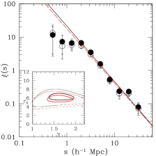
Figure 1: Comparison of the correlation function results based on the G05 random construction method (filled symbols) with that of the standard ‘sensitivity map’ method (empty symbols), applied on the AEGIS full band (0.5-8 keV) catalog. Uncertainties correspond to $1\sigma$ Poisson errors. The best fit power laws are shown as black lines for the G05 method and as dashed red lines for the sensitivity map method. In the inset panels we show the likelihood $1\sigma,2\sigma,3\sigma$ contours in the 2-parameter solution space. Right Panel: Redshift space correlation function, $\xi(s)$. Left Panel: Projected correlation function, $w_{p}(r_{p})$.

3.3 Random Catalogue Construction

To estimate the spatial correlation function of a sample of sources one needs to construct a large mock comparison sample with a random spatial distribution within the survey area, which also reproduces all the systematic biases that are present in the source sample (i.e., instrumental biases due to the Point Spread Function variation, vignetting, etc). Also special care has to be taken to reproduce any biases that enter through the optical counterpart spectroscopic observations strategy (cf., due to the positioning of the masks within the field of view and of the slits within the masks, etc).

To this end we will follow the random catalogue construction procedure of Gilli et al. (2005, hereafter G05), which is based on reshuffling only the source redshifts, smoothing the corresponding redshift distribution, while keeping the angular coordinates unchanged. We will test the efficiency of this method by comparing the outcome correlation function results with those of the standard method that takes into account the details of the sensitivity maps of each XMM pointing. We further test the two methods using N-body simulations for the underlying DM density field.

3.3.1 Random redshift reshuffling method

In order to assign random redshifts to the mock sample, the source redshift distribution is smoothed using a Gaussian kernel with a smoothing length of $\sigma_{z}=0.3$. This offers a compromise between scales that are either too small, and thus may reproduce the $z$-space clustering, or too large and thus over-smooth the observed redshift distribution. We verified that our results do not change significantly when using a smoothing length in the range $\sigma_{z}=0.2-0.4$.

3.3.2 Standard ‘sensitivity map’ method

According to the standard method of producing random catalogs, each simulated source is placed at a random position on the sky, with a flux randomly extracted from the observed source $\log N-\log S$ (source number-flux distribution). If the flux is above the value allowed by the sensitivity map at that position, the simulated source is kept in the random sample and a random redshift is also assigned to it from the observed source redshift distribution $N(z)$ (optimally taking into account the variation of $N(z)$ as a function of flux). The disadvantage of this method is that it does not take into account any unknown inhomogeneities and systematics of the follow-up spectroscopic observations.

3.3.3 Testing the efficiency of the two methods

In order to test the efficiency of the two random catalogue construction methods we use the AEGIS survey, consisting of 8 fields. To construct the standard method random catalogue we use the sensitivity maps of (Laird et al., 2009) and we compute the projected and redshift-space 2-point correlation functions. The best fit correlation length found is $r_{0}=4.28\pm 0.14~{}h^{-1}$ Mpc for $\gamma=1.8$ which is in excellent agreement with the results based on the G05 method: $r_{0}=4.13\pm 0.14~{}h^{-1}$ Mpc. In Fig. 1 we compare the correlation functions for the two random construction methods.

3.3.4 A further test using simulations

We use a 500 $h^{-1}$ Mpc cube simulation of a flat $\Omega_{m}=0.3$ and $\sigma_{8}=0.9$ cosmology with $512^{3}$ particles (Ragone-Figueroa & Plionis, 2007), to further test the robustness of the G05 random sample construction method. In order to have a relatively wide redshift range we replicate randomly the box to get an effective volume of $1500^{3}~{}h^{-3}$ Mpc³. To obtain a relatively large but manageable source density, we selected DM halos with $M_{\rm h}>1.5\times 10^{14}~{}h^{-1}M_{\odot}$, which resulted in a total number of haloes within our large simulation volume of $N=9\times 2312$.

We estimate the actual halo correlation function according to the direct method, which entails counting the number of DM halo pairs within spherical shells around a given halo. The corresponding number of random pairs is estimated by $\langle n\delta\rangle V$, with $\langle n\rangle$ the mean number density of halos in the whole simulation volume and $\delta V$ the volume of the spherical shell i.e. $4/3\pi\delta r^{3}$, with $\delta r$ being the width of the spherical shell.

We also estimate the halo correlation function using the G05 method, for which we transform the halo Cartesian coordinates into spherical coordinates, determining also their distance distribution. The clustering results of the two methods are in excellent agreement providing $\gamma=1.72(\pm 0.05)$ and $1.68(\pm 0.12)$ as well as $r_{0}=13.9(\pm 0.3)$ and $13.2(\pm 0.5)~{}h^{-1}$ Mpc, for the direct and G05 correlation function estimations, respectively.

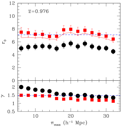
Figure 2: The resulting amplitude $r_{0}$, and slope $\gamma$, of the correlation function analysis as a function of the value of the $\pi_{\rm max}$ cutoff. The filled circles correspond to the results based on $w_{p}(r_{p})$, while the red squares on the results of $\xi(r_{p})$. The continuous red line corresponds to the crude estimation of the corrected spatial amplitude based on Eq. (7), while the dashed blue line correspond to the finally adopted results (which corresponds to the $\pi_{\rm max}=10~{}h^{-1}$ Mpc case).

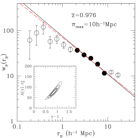
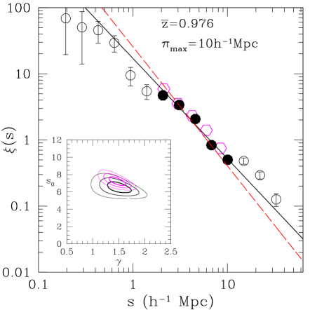
Figure 3: Correlation functions of the joint X-ray point-source sample: The projected correlation function, $w_{p}(r_{p})$ is shown in the upper panel, and the $z$-space correlation function, $\xi(s)$, is shown in the lower panel. The filled points indicate the range over which a power-law fit was applied (black line corresponds to a fit with free $\gamma$, while the red line to that for $\gamma=1.8$). The real-space correlation function, $\xi(r_{p})$ (via Eq. 6) is indicated in the lower panel by magenta pentagons. The inset panels show the 1, 2 and 3$\sigma$ likelihood contours in the 2-parameter plane of the power-law fit solutions.

4 RESULTS

4.1 The Joint X-ray Sample

Combining all five fields, we obtain in total 1466 X-ray sources with spectroscopic redshifts. The median redshift of the source sample is $\bar{z}=0.976$. In order to estimate the joint sample correlation function we generate random catalogs for each field separately and then combine them together. Note that we take care to count only once the sources that are common in both the CDF-S and eCDF-S fields.

We remind the reader that we fit a power-law to the measured correlation function over a range of separations for which such a model represents well the data. In order to avoid non-linear effects we use a lower separation limit, $r_{p}\simeq 1.5~{}h^{-1}$ Mpc, for the fit of $s$. We also impose an upper separation limit ($\simeq 10~{}h^{-1}$ Mpc) since we find a change above this scale in the slope of both projected and $z$-space correlation functions.

We now investigate the sensitivity of the correlation function on the cutoff separation along the line of sight, $\pi_{\rm max}$, which we vary in the range $[5,30]~{}h^{-1}$ Mpc. For $\pi_{\rm max}>30~{}h^{-1}~{}\rm{Mpc}$ the noise introduced by uncorrelated pairs reduces significantly the correlation function amplitude and slope. In Fig. (2) we show how the amplitude $r_{0}$ and the slope $\gamma$ of the projected correlation function, $w_{p}(r_{p})$ (open circles), and the corresponding real-space correlation function, $\xi(r_{p})$ (red squares), depend on $\pi_{\rm max}$. It is clear that both $r_{0}$ and $\gamma$ are relatively constant in the investigated $\pi_{\rm max}$ range. Our best fitting values for $r_{0}$ and $\gamma$ are those indicated by the dashed-blue line (see Table 1), which corresponds to $\pi_{\rm max}=10~{}h^{-1}$ Mpc.

Our main clustering results, based on the joint X-ray AGN sample, are shown in Fig. 3. The upper panel presents the projected correlation function, while the lower panel presents the redshift-space correlation function (circular points) as well as the inferred real-space correlation function, $\xi(r_{p})$, (magenta pentagons). The filled circular points are those which have been used to fit the power-law model correlation function, which is shown as a black continuous line (the dashed red line is the power-law fit for a fixed slope $\gamma=1.8$). The corresponding best fit values for the slope $\gamma$ and the correlation length are shown in Table 1. The uncertainty of $r_{0}$, indicated in Table 1, does not include the effects of cosmic variance, which can be estimated analytically, assuming a power-law correlation function, according to: $\sigma^{2}_{cv}\simeq J_{2}(\gamma)(r_{0}/r)^{\gamma}$, with $J_{2}(\gamma)=72/[(3-\gamma)(4-\gamma)(6-\gamma)2^{\gamma}]$ (Peebles, 1980). We find $\sigma_{cv}\simeq 0.3$, which is smaller although of the same order as the fitting uncertainty indicated in Table 1.

We can single out three important results from the clustering analysis of the joint X-ray point-source sample:

1. the inferred spatial correlation length, from the power-law model fit to Eq.  (6) or directly from Eq.  (7), is $\sim 20-25\%$ larger than that estimated from the projected correlation function, a fact which is attributed to the correlation function underestimation imposed by the necessary cutoff along the $\pi$ direction in the projected correlation function measure,

2. it appears that redshift-space distortions do not significantly affect the $z$-space correlation function, since $\xi(s)\simeq\xi(r_{p})$, and

3. the real-space correlation function, at a median redshift of 0.976, has a slope $\gamma\simeq 1.5$ and a correlation length $r_{0}\simeq 7.2~{}h^{-1}$ Mpc.

Table 1: Clustering results for the joint sample of all 5 fields (1466 sources). The clustering length units are $h^{-1}$ Mpc. The results correspond to $\pi_{\rm max}=10~{}h^{-1}$ Mpc, but they are very similar over the whole indicated $\pi_{\rm max}$ range, but more so for $5\raise-3.0pt\hbox{\hbox to0.0pt{\hbox{$\sim$}\hss}\raise 4.0pt\hbox{$<$}\ }\pi_{\rm max}\raise-3.0pt\hbox{\hbox to0.0pt{\hbox{$\sim$}\hss}\raise 4.0pt\hbox{$<$}\ }16~{}h^{-1}$ Mpc, as can be seen from Fig. 2. The cosmic variance is estimated to give a further $\sim 0.3$ uncertainty in $r_{0}$.

	$\gamma$	$r_{0}$	$r_{0}$ ($\gamma=1.8$)
$w_{p}(r_{p})$	1.84$\pm 0.07$	5.2$\pm 0.5$	$5.2\pm 0.5$
$\xi(s)$	1.49$\pm 0.20$	6.6$\pm 1.0$	$6.0\pm 0.8$
$\xi(r_{p})$	1.48$\pm 0.12$	7.2$\pm 0.6$	$6.5\pm 0.4$

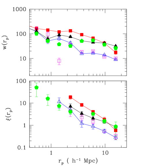
Figure 4: Correlation function of the individual X-ray surveys: CDF-N (green pentagons), CDF-S (red filled squares), eCDF-S (black filled triangles), COSMOS (magenta empty squares), AEGIS (blue empty triangles) for redshift interval $0<z<3$). Upper Panel: Projected correlation function. Lower Panel: The resulting spatial correlation function.

4.2 The Individual Field Correlation functions

We now perform the clustering analysis from the previous section in each individual field and compare our results to those from the original studies. To this end we use the redshift interval $0<z<3$ and sources with luminosities $L_{x}\geq 10^{41}$ erg s^-1, in order to avoid the gross contamination of our X-ray AGN sample by normal galaxies. We estimate the projected and $z$-space correlation functions in ten logarithmic intervals of width $\delta\log_{10}(r_{p},\pi)=0.175$ and $\delta\log_{10}(s)=0.2$, respectively. With the exception of the CDF-N field (see below), the power-law model fit was performed for $r_{p}\gtrsim 1.5~{}h^{-1}$ Mpc in order to avoid the non-linear contributions to the correlation function.

Table 2: Parameters of the power-law fits to the different survey correlation functions. The results of the projected correlation function, $w_{p}(r_{p})$, are shown in columns 4 and 5 and of the inferred real-space correlation function, $\xi(r_{p})$, in columns 6 and 7. Finally column 8 shows the correlation length of $\xi(r_{p})$ for the average value of the slope, $\gamma=1.44$ (which is practically equal to the slope of the joint sample, see Table 1). In all cases, except for the CDF-N, the power-law fits have been applied to the correlation function data, excluding the non-linear regime ($\raise-3.0pt\hbox{\hbox to0.0pt{\hbox{$\sim$}\hss}\raise 4.0pt\hbox{$<$}\ }1.5~{}h^{-1}$ Mpc). Since the CDF-N $w_{p}(r_{p})$ shows a knee around $r_{p}\sim 3.5~{}h^{-1}$ Mpc, we present power-law fits for data below and above this scale. Correlation lengths and $\pi_{\rm max}$ are in $h^{-1}$ Mpc.

Survey	$\#$	$\pi_{\rm max}$	$\gamma$	$r_{0}$	$\gamma_{c}$	$r_{0,c}$	$r^{\gamma=1.44}_{0,c}$
CDF-N1	243	20	$1.72\pm 0.30$	$4.6\pm 0.7$	$1.66\pm 0.16$	5.1$\pm 0.6$	6.0$\pm 0.8$
CDF-N2	243	20	$1.80\pm 0.23$	$9.9\pm 3.9$	$1.46\pm 0.22$	13.3$\pm 4.3$	13.3$\pm 4.3$
CDF-S	219	25	$1.90\pm 0.08$	$10.6\pm 1.4$	$1.72\pm 0.08$	12.8$\pm 1.1$	15.1$\pm 2.1$
AEGIS	392	20	$1.59\pm 0.09$	$4.3\pm 0.6$	$1.22\pm 0.20$	5.5$\pm 1.0$	5.7$\pm 0.8$
COSMOS	417	25	$1.65\pm 0.08$	$5.5\pm 0.8$	$1.36\pm 0.15$	6.8$\pm 1.0$	7.0$\pm 0.8$
eCDF-S	288	10	$1.46\pm 0.07$	$7.6\pm 1.0$	$1.23\pm 0.16$	12.4$\pm 2.2$	11.1$\pm 1.8$

• ¹ $r_{p}\raise-3.0pt\hbox{\hbox to0.0pt{\hbox{$\sim$}\hss}\raise 4.0pt\hbox{$<$}\ }3.5~{}h^{-1}$ Mpc

• ² $r_{p}>3.5~{}h^{-1}$ Mpc

In Fig. 4 we show the projected (upper panel) and the inferred via Eq. (6) spatial (lower panel) correlation function of the individual fields, color coded, while in Table 2 we summarize their best power-law fit parameters $\gamma$ and $r_{0}$. It is evident that the individual determinations of the correlation function are hampered by cosmic variance. It is also interesting to note that the results of the largest survey (COSMOS with $\sim 1$ deg² area) are consistent with those of the Joint sample (see Table 1).

We find small differences with respect to the results of the original studies, which are mostly due to the slightly different sample definitions and different choices of $\pi_{\rm max}$. For example, for the CDF-S field we use the $2~{}\rm{Msec}$ catalog rather than the $1~{}\rm{Msec}$ catalog used by Gilli et al. (2005), while for the CDF-N (Gilli et al., 2005) and for the AEGIS (Coil et al., 2009) samples, the corresponding authors used sources with $L_{x}\geq 10^{42}$ erg s^-1. When using the latter luminosity limit and the original value of $\pi_{\rm max}$, we recover the original clustering results. The only field for which it was not possible to fit a power-law correlation function in the linear scales is the CDF-N field, which presents a knee at $r_{p}\sim 3.5~{}h^{-1}$ Mpc. Therefore, we have performed a power-law fit in the two ranges where such is exhibited (i.e., for $r_{p}\raise-3.0pt\hbox{\hbox to0.0pt{\hbox{$\sim$}\hss}\raise 4.0pt\hbox{$<$}\ }3.5$ and $>3.5~{}h^{-1}$ Mpc, respectively).

The largest clustering amplitude is observed for the CDF-S, a fact which has been attributed to the existence of a large supercluster at $z\simeq 0.7$ (Gilli et al., 2003), and which appears to affect also the corresponding amplitude of the eCDF-S field, the correlation function of which is estimated here for the first time. However, inspecting Fig. 4 and Table 2, it is interesting to note that while the small-scale ($r_{p}\raise-3.0pt\hbox{\hbox to0.0pt{\hbox{$\sim$}\hss}\raise 4.0pt\hbox{$<$}\ }3.5~{}h^{-1}$ Mpc) correlation function of CDF-N is consistent with that of both the COSMOS and AEGIS fields, its large-scale correlation function ($r_{p}>3.5~{}h^{-1}$ Mpc) seems to be consistent with that of the CDF-S and eCDF-S fields. This suggests that either there is some unique structure affecting also the clustering pattern in the CDF-N (although at a lesser extent than in the CDF-S) or there is some unknown systematic affecting both CDF’s.

4.3 Luminosity Dependence of Clustering

We now wish to investigate the possibility of an X-ray luminosity dependent AGN clustering, as suggested by Plionis et al. (2008). Interestingly, Cappelluti et al. (2010), have found a dependence of clustering on the X-ray luminosity in the sample of local ($\langle z\rangle=0.05$) X-ray selected AGN from the SWIFT/BAT survey. Similarly, Krumpe et al. (2010) have also found such indications in the X-ray AGN sample from the ROSAT-All-sky-survey.

The five X-ray surveys that we have analysed in the previous sections, although they cover a similar redshift range, have X-ray luminosity distributions which are quite different. To disentangle the luminosity and redshift dependence of clustering, we construct a low-$L_{x}$ and a high-$L_{x}$ X-ray luminosity sub-sample for each survey. We also impose them to have the same redshift distribution. This is achieved by first splitting the sources according to the selected luminosity limit and then matching their binned redshift distribution in the common area. We do so by randomly selecting sources from the most abundant $L_{x}$ subsample so as to reproduce exactly the shape of the binned redshift distribution of the less abundant subsample. The bin size used is $\delta z=0.05$. This random selection process is performed eight times and the final results are the average over these eight realizations.

As an example of our procedure we show in Fig. 5 the redshift distribution of the whole AEGIS field (black thick line), dividing it also in its two luminosity subsamples, i.e., the low-$L_{x}$ with $L_{x}<10^{43}$ erg s^-1 (black dense-shaded histogram) and a high-$L_{x}$ with $L_{x}\geq 10^{43}$ erg s^-1 (red sparse-shaded histogram). In the inset panel we also show the X-ray luminosity distribution of the AEGIS field, were a clear division can be observed at $L_{x}\simeq 10^{43}$ erg s^-1. Finally, the left panel of Fig. 6 shows the redshift distribution of the low-$L_{x}$ and high-$L_{x}$ subsamples in the common redshift range ($0.5<z<1.5$), while in the right panel we present one random realization of the matched $z$-distributions of the two subsamples, which are those finally used to estimate the correlation function of the low-$L_{x}$ and high-$L_{x}$ subsamples. It is evident that our procedure has managed to create subsamples that have a common redshift distribution, therefore surpressing any redshift dependent effect in the comparison of the clustering results of the low and high-$L_{x}$ AGN subsamples.

Table 3: Correlation function results from the X-ray luminosity separated subsamples for each individual X-ray survey. Note that due to the small samples involved we have used different bin sizes for each sample, in order to minimize the intrinsic scatter. Note also that the following redshift intervals were used: CDF-N $0.5<z<1.2$; CDF-S $0.7<z<1.4$; AEGIS $0.5<z<1.5$; COSMOS $0.6<z<1.8$; eCDF-S $0.7<z<1.6$. The last two columns list the slope (averaged over the two luminosity sub-samples) and amplitude of the power-law fit to the spatial correlation function, $\xi(r_{p})$, of Eq. (6).

$\log_{10}L_{x}$	$\#$	$\bar{z}$	$\pi_{\rm max}$	$\gamma$	$r_{0}$	$\gamma_{c}$	$r_{0,c}$
CDF-N
$\leq 42.2$	73	0.84	10	$1.74\pm 0.15$	$3.4\pm 0.4$	1.36	$4.7\pm 0.7$
$>42.2$	79	0.96	10	$1.42\pm 0.16$	$4.5\pm 1.1$	1.36	$7.2\pm 1.1$
CDF-S
$\leq 42.5$	53	0.95	10	$1.97\pm 0.20$	$10.0\pm 2.5$	1.54	$16.5\pm 2.3$
$>42.5$	44	1.02	10	$1.65\pm 0.15$	$9.3\pm 2.3$	1.54	$13.6\pm 2.6$
AEGIS
$\leq 43$	90	0.83	20	$2.03\pm 0.29$	$4.6\pm 1.5$	1.83	$5.1\pm 1.3$
$>43$	63	0.82	20	$1.90\pm 0.30$	$5.7\pm 2.1$	1.83	$6.4\pm 1.8$
COSMOS
$\leq 43.5$	72	1.06	30	$2.00\pm 0.13$	$6.6\pm 1.3$	1.85	$7.6\pm 1.5$
$>43.5$	51	1.07	30	$2.00\pm 0.23$	$10.3\pm 3.0$	1.85	$11.9\pm 3.0$
eCDF-S
$\leq 43.2$	51	1.04	30	$1.91\pm 0.36$	$5.9\pm 2.5$	1.85	$6.3\pm 2.5$
$>43.2$	30	1.02	30	$1.98\pm 0.28$	$7.7\pm 3.0$	1.85	$8.6\pm 3.0$

We then use the $\chi^{2}$ minimization procedure to fit a power-law model to the measured $w_{p}(r_{p})$ of the low-$L_{x}$ and high-$L_{x}$ sub-samples, typically in the projected separation range $r_{p}\in[0.16-10]~{}h^{-1}$ Mpc. Note that it is not possible to exclude in this analysis the non-linear scales ($\raise-3.0pt\hbox{\hbox to0.0pt{\hbox{$\sim$}\hss}\raise 4.0pt\hbox{$<$}\ }1.5~{}h^{-1}$ Mpc) due to the small number of sources involved and the consequent noisy correlation function. Furthermore, and in order to be able to compare the different results on an equal footing, we present the inferred spatial correlation length, based on a power-law fit to the $\xi(r_{p})$ (Eq. 6) for a common slope, which is the mean of the low and high-$L_{x}$ sub-sample $\xi(r_{p})$ slopes.

The results of the correlation function analysis for the low and high-$L_{x}$ subsamples of the individual X-ray surveys can be found in Table 3. In Fig. 7 we present the inferred spatial clustering length, $r_{0,c}$, as a function of the X-ray luminosity. There are indications of a luminosity dependent clustering in all X-ray surveys, except for the CDF-S in which the correlation lengths for both low and high-$L_{x}$ subsamples are atypically very high (probably due to the dominance of a known supercluster, Gilli et al., 2003). Although the luminosity dependent clustering indications in each of the four remaining X-ray field are rather weak, there is an overall suggestive and systematic trend with the high $L_{x}$ subsamples being more strongly clustered than the lower $L_{x}$ ones. A linear least square fit to the data of Fig. 7, taking into account the uncertainties in both axes and excluding the CDF-S, provides the following dependence $r_{0,c}/(h^{-1}{\rm Mpc})\simeq 2.4\log_{10}L_{x}-94.7$. This is indicated by the thick continuous line in Fig. 7. The relatively strong trend implied by this relation, although the individual survey luminosity-dependence results are not that significant, is due to the fact that in each field a different high and low luminosity range is sampled, increasing the X-ray luminosity dynamical range.

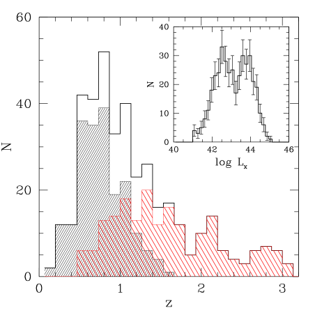
Figure 5: The redshift distribution of the AEGIS sources (thick black line histogram) divided also in the two luminosity subsamples (low-$L_{x}$: black dense-shaded histogram, and high-$L_{x}$: red sparse-shaded histogram). The inset panel shows the X-ray luminosity distribution. The trough between the two apparent peaks, at $L_{x}\simeq 10^{43}$ erg s^-1, defines the division value between the low-$L_{x}$ and high-$L_{x}$ subsamples.

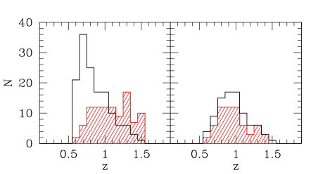
Figure 6: Left Panel: Redshift distribution at the common interval $z=0.5-1.5$ of the Low-$L_{x}$ (black line) and High-$L_{x}$ (red shade) subsamples. Right Panel: The matched redshift distributions of the further reduced subsamples, according to method described in the text imposed in order to cancel redshift dependent effects in their correlation function comparison.

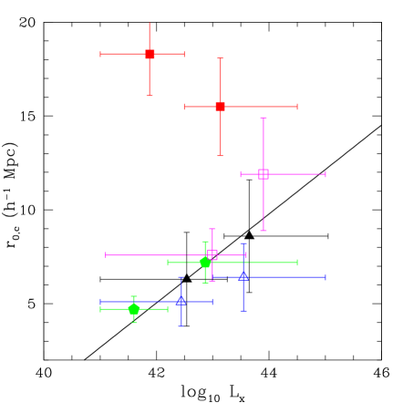
Figure 7: Spatial clustering length, $r_{0,c}$, estimated from Eq. (6), as a function of X-ray luminosity for the different surveys: The color code and symbols are the same as in Fig. 4. The black line is the best linear fit to the data, excluding the CDF-S (red circles) results.

5 BIAS AND HOST HALO MASS

It is well established that the extragalactic sources are biased tracers of the underlying mass fluctuation field (e.g., Kaiser, 1987; Bardeen et al., 1986). The parameter that encapsulates this fact is the so-called linear bias factor, $b$, defined as the ratio of the fluctuations of some mass tracer, here the AGN ($\delta_{\rm AGN}$), to those of the underlying DM mass ($\delta_{\rm DM}$),

$$b=\frac{\delta_{\rm AGN}}{\delta_{\rm DM}}\;.$$ (10)

Since the correlation function is generally defined as $\xi(r)=\langle\delta({\bf x})\delta({\bf x}+{\bf r})\rangle$ (the so-called Poisson-process definition), an equivalent definition of the bias parameter is the square root of the ratio of the two-point correlation function of AGN to that of the underlying mass,

$$b=\left(\frac{\xi_{\rm AGN}}{\xi_{\rm DM}}\right)^{1/2}.$$ (11)

Another related definition, which is the one that will be used in the current work, is as the ratio of the variances of the AGN and underlying mass density fields, smoothed at some linear scale,

$$b=\frac{\sigma_{8,\rm AGN}}{\sigma_{8,\rm DM}};,$$ (12)

where $\sigma_{8,\rm AGN}$ is the rms fluctuations of the AGN density distribution within spheres of a co-moving radius of $8~{}h^{-1}$ Mpc, given under the assumption of power-law correlations, by Peebles (1980),

$$\sigma_{8,\rm AGN}=J_{2}(\gamma)^{\frac{1}{2}}\left(\frac{r_{0}}{8}\right)^{\frac{\gamma}{2}}\;,$$ (13)

and $\sigma_{8,\rm DM}$ is the variance of the DM density fluctuation field which evolves according to (e.g., Peebles 1993):

$$\sigma_{8,\rm DM}(z)=\sigma_{8}\frac{D(z)}{D(0)}\;,$$ (14)

with $D(z)$ the linear growth factor, which for the concordance $\Lambda$ cosmology is given by (Peebles 1993)

$$D(z)=\frac{5\Omega_{m}E(z)}{2}\int_{z}^{\infty}\frac{(1+y)}{E^{3}(y)}\mathrm{d}y\;.$$ (15)

Combining Eqs. (12), (13), (14), we obtain the cosmological evolution of biasing as a function of the power-law clustering parameters,

$$b(z)=\left(\frac{r_{0}}{8}\right)^{\frac{\gamma}{2}}J_{2}^{\frac{1}{2}}\left(\frac{\sigma_{8}D(z)}{D(0)}\right)^{-1}.$$ (16)

Finally, an alternative approach to estimate the bias, free of the power-law clustering assumption, is provided by the square-root of the ratio of the projected AGN correlation function to the two-halo term of the theoretical projected correlation function, based on the Fourier transform of the linear CDM power-spectrum (eg., Allevato et al. 2011; Krumpe et al. 2012). These authors have used both of the latter two apporaches to estimate the bias and have shown that they provide mutually consistent results.

The CDM structure formation scenario predicts that the bias factor is determined by the mass of the DM halo within which the extragalactic mass tracer forms (e.g., Mo & White, 1996). In order to assign a characteristic DM halo mass to the estimated bias factors we use two bias evolution models, the Tinker et al. (2010) (hereafter TRK) and the Basilakos et al. (2008) model (hereafter BPR). The former, an improvement of the original Sheth & Tormen (1999) model, belongs to the so-called galaxy merging bias family, which is based on the Press & Schechter (1974) formalism, the peak-background split (Bardeen et al., 1986) and the spherical collapse model (e.g., Sheth & Tormen, 1999; Valageas, 2009, 2011). The latter is an extension of the so-called galaxy conserving bias models, and uses linear perturbation theory, and the Friedmann-Lemaitre solutions to derive a second-order differential equation for the evolution of bias, assuming that the tracer and the underlying mass share the same dynamics. Furthermore, the model includes the contribution of an evolving DM halo population, due to processes like merging. Details of these models, as well as a comparison among five current bias evolution models can be found in Papageorgiou et al. (2012).

5.1 X-ray AGN Bias

Table 4: The bias corresponding to the clustering of the Joint sample (1466 sources) and of the luminosity divided subsamples for each individual X-ray survey studied. The corresponding values of the halo mass, in units of $\log_{10}(M_{\rm h}/[h^{-1}M_{\odot}])$, are estimated using a WMAP7 cosmology, i.e., $\sigma_{8}=0.81$ and $\Omega_{m}=0.273$ and are based on the BPR (4th column) and TRK (5th column) bias evolution model.

$\log_{10}L_{x}$	$\overline{\log_{10}L_{x}}$	$\bar{z}$	$b(\bar{z})$	BPR	TRK
JOINT
		0.98	$2.26\pm 0.16$	$13.06^{+0.12}_{-0.14}$	$13.19^{+0.07}_{-0.09}$
CDF-N
$\leq 42.2$	41.84	0.84	$1.52\pm 0.17$	$12.38^{+0.29}_{-0.40}$	$12.26^{+0.23}_{-0.30}$
$>42.2$	43.18	0.96	$2.15\pm 0.24$	$12.99^{+0.20}_{-0.24}$	$12.79^{+0.19}_{-0.21}$
CDF-S
$\leq 42.5$	42.19	0.95	$4.22\pm 0.47$	$14.07^{+0.15}_{-0.17}$	$13.86^{+0.11}_{-0.12}$
$>42.5$	43.45	1.02	$3.75\pm 0.56$	$13.80^{+0.20}_{-0.25}$	$13.52^{+0.17}_{-0.21}$
AEGIS
$\leq 43$	42.75	0.89	$1.74\pm 0.41$	$12.65^{+0.45}_{-0.84}$	$12.49^{+0.39}_{-0.64}$
$>43$	43.86	0.89	$2.14\pm 0.55$	$13.09^{+0.41}_{-0.68}$	$12.87^{+0.35}_{-0.57}$
COSMOS
$\leq 43.5$	43.30	1.07	$2.72\pm 0.50$	$13.24^{+0.27}_{-0.36}$	$13.04^{+0.24}_{-0.33}$
$>43.5$	44.21	1.07	$4.12\pm 0.96$	$13.86^{+0.29}_{-0.39}$	$13.59^{+0.24}_{-0.34}$
eCDF-S
$\leq 43.2$	42.86	1.03	$2.25\pm 0.83$	$12.96^{+0.54}_{-1.16}$	$12.79^{+0.47}_{-0.97}$
$>43.2$	43.97	1.03	$3.00\pm 0.97$	$13.46^{+0.42}_{-0.70}$	$13.22^{+0.37}_{-0.62}$

When applying the above analysis to the clustering results of our Joint X-ray sample (with a median redshift $\langle z\rangle\simeq 0.98$), we find a bias factor of $b\simeq 2.26\pm 0.16$. This value corresponds to a DM halo mass of $\log_{10}(M_{\rm h}/h^{-1}M_{\odot})\simeq 13.06(\pm 0.13)$ and 13.19$(\pm 0.08)$ for the BPR and TRK models, respectively (the first raw of Table 4). We also extend the same analysis to the low-$L_{x}$ and high-$L_{x}$ AGN subsamples in each X-ray field separately. As expected by the dependence of the correlation function on luminosity that we presented in Section 4.3, the high-$L_{x}$ subsamples provide larger bias factors and correspondingly larger DM halo masses (for both the BPR and TRK bias models) than those of the low-$L_{x}$ subsamples. An exception is the CDF-S field, which as we have already discussed, is hampered by the presence of a large supercluster; Gilli et al. (2003). Thus, the data seem to suggest that high-$L_{x}$ sources inhabit more massive DM halos than low-$L_{x}$ sources. The results listed in Table 4 indicate that for an average luminosity difference of $\langle\delta\log_{10}L_{x}\rangle\simeq 1$ between the high and low-$L_{x}$ AGN subsamples, the corresponding average DM halo mass of the former sample is a factor of $\sim 3$ larger than that of the latter.

Similar results have been found by Cappelluti et al. (2010), for a sample of X-ray selected AGN from the SWIFT/BAT survey. The authors derive for AGN with $\rm L_{x}<10^{44}\rm{~{}erg~{}s}^{-1}$ a DM host halo mass of $\log_{10}(M_{\rm h}/[h^{-1}M_{\odot}])\approx 10^{12}M_{\odot}$, while for AGN with $L_{x}\geq 10^{44}\rm{~{}erg~{}s}^{-1}$ they find a DM host halo mass of $\sim 10^{14}~{}h^{-1}M_{\odot}$. Krumpe et al. (2010) also find evidence for luminosity dependence in a sample of the ROSAT-All-sky-survey AGN. In particular, they find $\log_{10}(M_{\rm h}/[h^{-1}M_{\odot}])=11.83$ and $13.10$ for their low and high X-ray luminosity AGN sources (below and above $L_{0.1-2.4{\rm keV}}=10^{44.3}\rm{~{}erg~{}s}^{-1}$), respectively.

5.2 Bias Evolution

Table 5: The values of the X-ray AGN bias factor in redshift bins. Above $z=2$ the correlation function was extremely noisy and impossible to determine. The halo mass shown are estimated using a WMAP7 cosmology, i.e., $\sigma_{8}=0.81$ and $\Omega_{m}=0.273$ and for three different models of bias evolution (see also Papageorgiou et al. 2012).

$\#$	$z$-range	$\bar{z}$	$b(\bar{z})$	$\log_{10}(M_{\rm~{}h}/h^{-1}M_{\odot})$
				BPR	TRK
353	0.00 - 0.67	0.488	$1.71\pm 0.23$	$13.37^{+0.27}_{-0.36}$	$13.00^{+0.21}_{-0.29}$
354	0.67 - 0.96	0.787	$2.46\pm 0.25$	$13.52^{+0.16}_{-0.19}$	$13.22^{+0.14}_{-0.16}$
352	0.96 - 1.38	1.123	$2.46\pm 0.23$	$13.00^{+0.16}_{-0.18}$	$12.90^{+0.10}_{-0.22}$
200	1.38 - 2.00	1.613	$3.85\pm 1.55$	$13.09^{+0.48}_{-0.88}$	$13.00^{+0.43}_{-0.82}$

In order to investigate the redshift evolution of the bias factor we split the whole sample in four redshift bins. The resulting values of the bias factor in each bin, as well the typical DM halo masses, based on the two previously mentioned models, are shown in Table 5. Fig. 8 (left panel) shows our determination of the bias in the different redshift bins together with the corresponding results of the XMM-COSMOS (Allevato et al., 2011), the XBOOTES (Starikova et al., 2011), the ROSAT (Krumpe et al., 2010) and SWIFT/BAT (Cappelluti et al. (2010)) surveys. The increase of the bias factor with increasing redshift is evident, as well as the consistency of the derived bias values of the different studies at the corresponding redshifts.

Allevato et al. (2011) has argued that models of bias evolution based on a single host halo mass cannot explain their results, but rather there are indications for different halo masses hosting X-ray AGN at the different redshifts. We check their suggestion by applying the previously mentioned bias-evolution models, and attempting to fit a single halo mass jointly to all the previously mentioned bias data. Indeed no such model can fit adequately well the results (the resulting reduced $\chi^{2}$ is $\raise-3.0pt\hbox{\hbox to0.0pt{\hbox{$\sim$}\hss}\raise 4.0pt\hbox{$>$}\ }1.6$). The cause of this failure is mostly the deviant bias values around $z\sim 0.75$. If this redshift bin is excluded, then the bias data can indeed be fitted by a single host halo mass with $\log_{10}(M_{\rm h}/[h^{-1}M_{\odot}])\simeq 13.06\pm 0.04$, $\chi^{2}$/df$=0.24$ and a present epoch bias of $b(0)=1.1$ (black continuous line in Fig. 8) for the BPR model. For the TRK model we find $\log_{10}(M_{\rm h}/[h^{-1}M_{\odot}])\simeq 12.94\pm 0.05$, $\chi^{2}$/df$=0.48$ and $b(0)=1.18$ (black dashed line in Fig. 8). If we use however, only the three deviant bias values around $z\simeq 0.75$, we find $\log_{10}(M_{\rm h}/[h^{-1}M_{\odot}])\simeq 13.56\pm 0.09$, $\chi^{2}$/df$=0.29$ and $b(0)=1.24$ (magenta continuous line) for the BPR model, and $\log_{10}(M_{\rm h}/[h^{-1}M_{\odot}])\simeq 13.28\pm 0.10$, $\chi^{2}$/df$=0.29$ and $b(0)=1.39$ (magenta dashed line) for the TRK model. It is interesting to point out that the bias values of the current study (red pentagons), when excluding the deviant point, provide exactly the same fit as the one obtained previously, using all the determinations of the bias evolution values (again excluding the deviant points). However, the uncertainty is, as expected, larger (for example, for the BPR model we obtain $\log_{10}(M_{\rm h}/[h^{-1}M_{\odot}])\simeq 13.08\pm 0.14$ with a $\chi^{2}$/df$=0.48$).

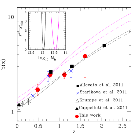
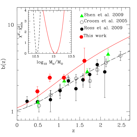
Figure 8: Left Panel: Comparison of the redshift evolution of the bias parameter of our Joint X-ray sample (red pentagons), with that of other X-ray surveys. The point and color coding of the results based on different surveys is indicated by the corresponding labels. The theoretical bias evolution models, fitted to the data for a single DM halo mass, are shown as continuous or dashed lines: The black continuous line is the best fit BPR bias evolution model to all the bias data, excluding the deviant points at $z\sim 0.75$, while the dashed line is the corresponding best fit TRK model. The magenta continuous and dashed lines are the fits of the corresponding two models to the bias values around $z\sim 0.75$. In the inset panel we show the best fit DM halo mass value as a function of $\chi^{2}-\chi_{min}^{2}$ for the BPR model. A value of $\chi^{2}-\chi_{min}^{2}=1$ or 4 correspond to the 1 and 2$\sigma$ uncertainty in the fitted parameter (for the case of one free parameter). Right Panel: Comparison of the redshift evolution of the bias parameter of the Joint X-ray sample (red pentagons), to that of optical QSOs. The point and color coding of the results based on different surveys is indicated by the corresponding labels. The curves correspond to the BPR bias evolution model fitted to the X-ray data (red continuous line) and to the optical QSO (black dashed line). Note that the plotted bias values are rescaled to the WMAP7 cosmology, as in Papageorgiou et al. (2012).

5.3 X-ray versus Optically selected AGN

We also compare in the right panel of Fig. 8 our X-ray AGN results with the bias of optically selected QSO, based on the 2dF spectroscopic sample of 20000 QSOs (Croom et al., 2005), on an SDSS (DR5) QSO sample of $\sim$30000 spectroscopic QSO with $z\raise-3.0pt\hbox{\hbox to0.0pt{\hbox{$\sim$}\hss}\raise 4.0pt\hbox{$<$}\ }2.2$ (Ross et al., 2009) and on a homogeneous sample of $\sim$38000 SDSS QSOs with $0.1\leq z\leq 5$ (Shen et al., 2009). Since the X-ray data do not extend to such high redshifts and in order to consistently compare optical and X-ray bias data, we choose to exclude the very high-$z$ (3$<z<4.5$) optical bias data of Shen et al. Note also that since each of the optical QSO studies have used a slightly different flat $\Lambda$CDM background cosmology, the bias values shown in Fig. 8 have been scaled to the WMAP7 cosmology, following the prescription of Papageorgiou et al. (2012). The results of each of the different studies are indicated in the Figure with distinct colours and symbol types.

The BPR model that fits simultaneously all the optical QSO bias data, provides a DM halo mass of $\log_{10}(M_{\rm h}/[h^{-1}M_{\odot}])\simeq 12.50\pm 0.05$ with $\chi^{2}/$df$=0.68$. The corresponding values for the TRK bias model are practically the same: $\log_{10}(M_{\rm h}/[h^{-1}M_{\odot}])\simeq 12.49\pm 0.04$ with $\chi^{2}/$df$=0.64$. It is therefore evident that the X-ray selected AGN bias values, and the corresponding DM halo masses, are significantly larger than those of the optical QSO, indicating that they probably constitute separate families of AGN, each probably having a distinct BH fueling mechanism. Allevato et al. (2011) also conclude that the DM halos in which X-ray selected AGN reside are more massive than those of optically selected QSOs. Further below we will provide a tentative explanation for such a difference between the host halos of optical and X-ray selected AGN.

6 Comparison with AGN accretion models

Our analysis provides new insights into the host DM halos of moderate luminosity X-ray selected AGN. By fitting two different bias evolution models, we find that the AGN in our samples inhabit DM halos with masses of $\log_{10}(M_{\rm h}/[h^{-1}M_{\odot}])\simeq 13.1\pm 0.1$. The estimated halo mass is significantly higher than the typical halo mass of optically selected QSO [$\log_{10}(M_{\rm h}/[h^{-1}M_{\odot}])\sim 12.5$; see Fig. 8]. Similar results are also found in other X-ray studies (e.g. Coil et al., 2009; Starikova et al., 2011), (Allevato et al., 2011; Mountrichas & Georgakakis, 2012) and therefore the DM halos masses estimated in most X-ray surveys are consistent mostly with those of elliptical/red galaxies. This implies that the fueling mechanism of the moderate luminosity X-ray selected AGN and the more luminous optically selected QSOs is different.

Semi-analytic models that assume major mergers as the main mechanism for triggering AGN activity predict that the mass of DM halos that host AGN is lower than that estimated from observations of moderate luminosity X-ray AGN (e.g., Marulli et al., 2009; Bonoli et al., 2009). The theoretical predictions from these models are more consistent with the halo mass of optically selected QSOs. Additional evidence against the major mergers scenario in moderate luminosity X-ray AGN comes from the morphological analysis of AGN in the AEGIS and COSMOS surveys (Georgakakis et al., 2009; Silverman et al., 2009). These authors find that X-ray selected AGN span a large range of environments and morphologies with roughly equal numbers of bulges, spirals and morphologically disturbed galaxies (see also Schawinski et al., 2011; Kocevski et al., 2012; Cisternas et al., 2011). Also stochastic accretion models (Hopkins & Hernquist, 2006) cannot explain large DM halos for moderate luminosity AGN. According to these models, disc instabilities and minor interactions feed at high accretion rates relatively small black holes. These models predict that moderate luminosity AGN reside in low density environments, similar to those of blue star-forming galaxies.

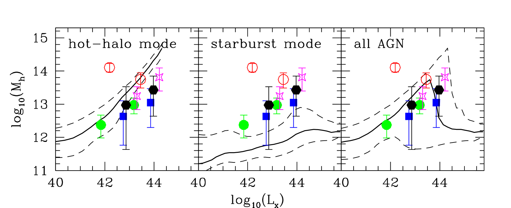
Figure 9: The median X-ray luminosity (0.5-8 keV) of the luminosity separated subsamples (from Table 4) vs. the DM halo mass predicted by the TRK bias model. The color coding is same as in Fig.  4. For comparison we show the theoretical predictions of the Fanidakis et al. (2012) black hole model at $z=0.5-1.5$. Solid lines indicate the median of the $\log L_{\rm x}-\log M_{\rm h}$ correlation for AGN accreting from the hot halo (hot-halo mode; left panel), or during disc instabilities and mergers (starburst mode; middle panel) and all AGN in their model (right panel). The dashed lines indicate the $10-90$ percentiles around the median.

Regarding the luminosity dependence of the clustering of X-ray selected AGN (and consequent luminosity dependence of the host halo mass) various theoretical models of black hole and galaxy co-evolution predict only a weak dependence of AGN clustering on luminosity, (e.g., Lidz et al., 2006; Hopkins et al., 2005; Hopkins & Hernquist, 2006). In these models, both the bright and faint AGN reside in similar mass halos. The bright AGN correspond to black holes that radiate at their peak luminosities, i.e. at accretion rates close to the Eddington ones. In contrast, the faint end of the AGN luminosity function consists of AGN in dimmer (late) phases in their evolution.

Our derived DM halo masses of X-ray selected AGN could suggest, as Mountrichas & Georgakakis (2012) also point out, a fueling mechanism similar to that of Ciotti & Ostriker (2001). The authors suggest that stellar winds in early-type galaxies provide the gas supply to the black hole (see also Kauffmann & Heckman 2009). Alternatively, another plausible model is that of Bower et al. (2006), where gas is accreted onto BHs directly from the hot halo of the galaxy. Fanidakis et al. (2012), recently presented a calculation for accreting black holes within the Bower et al. (2006) semi-analytic model, where AGN activity is coupled to the evolution of the host galaxy. The authors assume that black holes grow via accretion triggered by galaxy mergers and disk instabilities (starburst mode), as well as accretion of hot gas from the halo of the galaxy (hot-halo mode). In Fig.9, we compare our halo mass estimates for the individual subsamples in Table 5 with the predictions of the Fanidakis et al. (2012) model for the $L_{x}-M_{h}$ correlation at $z=0.5-1.5$. Their calculations assume a flat cosmology with $\Omega_{m}=0.25$, $\Omega_{b}=0.045$, $\sigma_{8}=0.9$ and $h=0.7$, and for consistency, we re-estimated the DM halo mass values according to their adopted cosmology.

As illustrated by the left panel of Fig.  9, the Fanidakis et al. model predicts a strong X-ray luminosity – halo mass correlation for AGN accreting in the hot-halo mode. In contrast, the halo mass of AGN in the starburst mode shows a very modest increase to X-ray luminosities of $L_{\rm X}\simeq 10^{44}\rm{ergs^{-1}}$, beyond which it remains constant and approximately equal to $10^{12}\rm{M_{\odot}}$ (middle panel). When considering all the AGN in the model, the shape of the correlation is dominated by the hot-halo mode in the low-luminosity and by the starburst mode in the high-luminosity regime (right panel). Thus, the resulting correlation increases steeply in the moderate luminosity regime and then sharply declines and flattens for the brightest luminosities. Our X-ray selected AGN results appear to be in very good agreement with the predictions of the Fanidakis et al. model. The data lie in the region of the $L_{\rm X}-M_{\rm h}$ plane, which is dominated by the hot-halo mode. This suggests that intermediate luminosity AGN are preferentially powered by accretion of gas from the hot halo. Their model further proposes that sources with $L_{\rm X}\gtrsim 10^{44}\rm{ergs^{-1}}$, expected to be visible as QSOs, live in haloes with masses of $\sim 10^{12}M_{\odot}$ as suggested by clustering studies of optically selected QSOs (see Fig. 8, right panel).

The distinctive environmental dependence of the starburst and hot-halo mode in the Fanidakis et al. model is linked to the cooling properties of the gas in DM haloes (White & Frenk, 1991). In the starburst mode, disc instabilities and galaxy mergers take place in gas rich environments. In the standard $\Lambda$CDM paradigm, this corresponds to intermediate mass DM haloes, where gas cools rapidly. In more massive haloes, the gas is in quasi-hydrostatic equilibrium and therefore characterized by a significant lower cooling efficiency. In addition, in this mass regime AGN feedback reheats the gas in the halo, shutting off the cooling completely. AGN activity maximizes at the transition between the rapid-cooling and quasi-hydrostatic regime, which in the Fanidakis et al. model is found to take place at $M_{\rm h}\sim 10^{12}M_{\odot}$. In haloes more massive than $\sim 10^{12}M_{\odot}$, black holes accrete low-density gas directly from the hot halo. In this case, the authors assume that the amount of gas that is accreted onto the BH is determined by, and in fact is proportional to the cooling luminosity of the gas in the halo (see Bower et al., 2006; Fanidakis et al., 2011). Since the cooling luminosity increases with increasing halo mass, their model predicts a strong correlation between accretion luminosity and DM halo mass. The good agreement of the predictions of these accretion prescriptions with our analysis, but also with the clustering results of optically selected QSOs, strengthens the idea of two distinct fueling modes; the hot-halo mode in moderate X-ray AGN and the starburst mode in the more luminous optical QSOs.

7 SUMMARY

We use 1466 X-ray selected AGN in the 0.5-8 keV band with spectroscopic redshifts spanning the redshift interval $0<z<3$, with a median of $\bar{z}=0.976$. We derive a spatial clustering length of $r_{0}=7.2\pm 0.6h^{-1}$ Mpc and a slope of $\gamma=1.47\pm 0.12$. The corresponding clustering length for the nominal slope of $\gamma=1.8$ is $r_{0}=6.5\pm 0.4~{}h^{-1}$ Mpc. The above clustering length corresponds to a bias of $b(\bar{z})=2.26\pm 0.16$, translating to a mass of the host DM halo of $M_{\rm h}\sim 1.3\times 10^{13}~{}h^{-1}M_{\odot}$. The derived bias and the corresponding host halo mass of X-ray selected AGN is significantly higher than that of optically selected AGN. This may imply a different fueling mechanism for X-ray selected AGN in comparison to optically selected AGN. We also find indications for a dependence of the clustering strength on the X-ray luminosity, when we consider AGN at a redshift of $z\sim 1$. The more X-ray luminous the sources are the larger, typically, the clustering length and hence the higher the DM host halo mass is. For an average luminosity difference of $\langle\delta\log_{10}L_{x}\rangle\simeq 1$, between the high and low-$L_{x}$ AGN subsamples, the corresponding average DM halo mass of the former sample is a factor of $\sim 3$ larger than that of the latter.

The luminosity-dependent clustering that we find seems to be in favor of a black hole accretion model where moderate luminosity X-ray AGN, at $z\sim 1$, are fueled mostly by accretion from the hot halo around the host galaxy. The good agreement of the model predictions with similar studies in the optical further suggests that luminous quasar activity is triggered in lower-mass halo (and gas-rich) environments by disk instabilities and galaxy mergers.

References

- Akylas et al. (2000) Akylas A., Georgantopoulos I., Plionis M., 2000, MNRAS, 318, 1036
- Alexander et al. (2003) Alexander D. M., Bauer F. E., Brandt W. N., Schneider D. P., Hornschemeier A. E., Vignali C., Barger A. J., Broos P. S., Cowie L. L., Garmire G. P., Townsley L. K., Bautz M. W., Chartas G., Sargent W. L. W., 2003, AJ, 126, 539
- Allevato et al. (2011) Allevato V., Finoguenov A., Cappelluti N., Miyaji T., Hasinger G., Salvato M., Brusa M., Gilli R., Zamorani G., Shankar F., James J. B., McCracken H. J., Bongiorno A., Merloni A., Peacock J. A., Silverman J., Comastri A., 2011, ApJ, 736, 99
- Bardeen et al. (1986) Bardeen J. M., Bond J. R., Kaiser N., Szalay A. S., 1986, ApJ, 304, 15
- Basilakos et al. (2004) Basilakos S., Georgakakis A., Plionis M., Georgantopoulos I., 2004, ApJ, 607, L79
- Basilakos et al. (2005) Basilakos S., Plionis M., Georgakakis A., Georgantopoulos I., 2005, MNRAS, 356, 183
- Basilakos et al. (2008) Basilakos S., Plionis M., Ragone-Figueroa C., 2008, ApJ, 678, 627
- Bonoli et al. (2009) Bonoli S., Marulli F., Springel V., White S. D. M., Branchini E., Moscardini L., 2009, MNRAS, 396, 423
- Bournaud et al. (2011) Bournaud F., Dekel A., Teyssier R., Cacciato M., Daddi E., Juneau S., Shankar F., 2011, ApJ, 741, L33
- Bower et al. (2006) Bower R. G., Benson A. J., Malbon R., Helly J. C., Frenk C. S., Baugh C. M., Cole S., Lacey C. G., 2006, MNRAS, 370, 645
- Brusa et al. (2010) Brusa M., Civano F., Comastri A., Miyaji T., Salvato M., Zamorani G., Cappelluti N., Fiore F., Hasinger G., Mainieri V., Merloni A., Bongiorno A., Capak P., Elvis M., Gilli, 2010, ApJ, 716, 348
- Cappelluti et al. (2010) Cappelluti N., Ajello M., Burlon D., Krumpe M., Miyaji T., Bonoli S., Greiner J., 2010, ApJ, 716, L209
- Carrera et al. (2007) Carrera F. J., Ebrero J., Mateos S., Ceballos M. T., Corral A., Barcons X., Page M. J., Rosen S. R., Watson M. G., Tedds J. A., Della Ceca R., Maccacaro T., Brunner H., Freyberg M., Lamer G., Bauer F. E., Ueda Y., 2007, A&A, 469, 27
- Ciotti & Ostriker (2001) Ciotti L., Ostriker J. P., 2001, ApJ, 551, 131
- Cisternas et al. (2011) Cisternas M., Jahnke K., Inskip K. J., Kartaltepe J., Koekemoer A. M., Lisker T., Robaina A. R., Scodeggio M., Sheth K., Trump J. R., Andrae R., Miyaji T., Lusso E., Brusa M., Capak P., Cappelluti N., Civano F., Ilbert O., Impey C. D., Leauthaud A., Lilly S. J., Salvato M., Scoville N. Z., Taniguchi Y., 2011, ApJ, 726, 57
- Coil et al. (2009) Coil A. L., Georgakakis A., Newman J. A., Cooper M. C., Croton D., Davis M., Koo D. C., Laird E. S., Nandra K., Weiner B. J., Willmer C. N. A., Yan R., 2009, ApJ, 701, 1484
- Croom et al. (2005) Croom S. M., Boyle B. J., Shanks T., Smith R. J., Miller L., Outram P. J., Loaring N. S., Hoyle F., da Ângela J., 2005, MNRAS, 356, 415
- Croton et al. (2006) Croton D. J., Springel V., White S. D. M., De Lucia G., Frenk C. S., Gao L., Jenkins A., Kauffmann G., Navarro J. F., Yoshida N., 2006, MNRAS, 365, 11
- da Ângela et al. (2008) da Ângela J., Shanks T., Croom S. M., Weilbacher P., Brunner R. J., Couch W. J., Miller L., Myers A. D., Nichol R. C., Pimbblet K. A., de Propris R., Richards G. T., Ross N. P., Schneider D. P., Wake D., 2008, MNRAS, 383, 565
- Davis et al. (2003) Davis M., Faber S. M., Newman J., Phillips A. C., Ellis R. S., Steidel C. C., Conselice C., Coil A. L., Finkbeiner, 2003, in Society of Photo-Optical Instrumentation Engineers (SPIE) Conference Series, Vol. 4834, Society of Photo-Optical Instrumentation Engineers (SPIE) Conference Series, Guhathakurta P., ed., pp. 161–172
- Davis et al. (2001) Davis M., Newman J. A., Faber S. M., Phillips A. C., 2001, in Deep Fields, Cristiani S., Renzini A., Williams R. E., eds., p. 241
- Davis & Peebles (1983) Davis M., Peebles P. J. E., 1983, ApJ, 267, 465
- Di Matteo et al. (2005) Di Matteo T., Springel V., Hernquist L., 2005, in Growing Black Holes: Accretion in a Cosmological Context, Merloni A., Nayakshin S., Sunyaev R. A., eds., pp. 340–345
- Ebrero et al. (2009) Ebrero J., Mateos S., Stewart G. C., Carrera F. J., Watson M. G., 2009, A&A, 500, 749
- Elvis et al. (2009) Elvis M., Civano F., Vignali C., Puccetti S., Fiore F., Cappelluti N., Aldcroft T. L., Fruscione A., Zamorani G., Comastri, 2009, ApJ, 184, 158
- Elyiv et al. (2012) Elyiv A., Clerc N., Plionis M., Surdej J., Pierre M., Basilakos S., Chiappetti L., Gandhi P., Gosset E., Melnyk O., Pacaud F., 2012, AAP, 537, A131
- Fanidakis et al. (2011) Fanidakis N., Baugh C. M., Benson A. J., Bower R. G., Cole S., Done C., Frenk C. S., 2011, MNRAS, 410, 53
- Fanidakis et al. (2012) Fanidakis N., Baugh C. M., Benson A. J., Bower R. G., Cole S., Done C., Frenk C. S., Hickox R. C., Lacey C., Del P. Lagos C., 2012, MNRAS, 419, 2797
- Ferrarese & Ford (2005) Ferrarese L., Ford H., 2005, SSR, 116, 523
- Gandhi et al. (2006) Gandhi P., Garcet O., Disseau L., Pacaud F., Pierre M., Gueguen A., Alloin D., Chiappetti L., Gosset E., Maccagni D., Surdej J., Valtchanov I., 2006, A&A, 457, 393
- Georgakakis et al. (2009) Georgakakis A., Coil A. L., Laird E. S., Griffith R. L., Nandra K., Lotz J. M., Pierce C. M., Cooper M. C., Newman J. A., Koekemoer A. M., 2009, MNRAS, 397, 623
- Gilli et al. (2003) Gilli R., Cimatti A., Daddi E., Hasinger G., Rosati P., Szokoly G., Tozzi P., Bergeron J., Borgani S., Giacconi R., Kewley L., Mainieri V., Mignoli M., Nonino M., Norman C., Wang J., Zamorani G., Zheng W., Zirm A., 2003, ApJ, 592, 721
- Gilli et al. (2005) Gilli R., Daddi E., Zamorani G., Tozzi P., Borgani S., Bergeron J., Giacconi R., Hasinger G., Mainieri V., 2005, A&A, 430, 811
- Gilli et al. (2009) Gilli R., Zamorani G., Miyaji T., Silverman J., Brusa M., Mainieri V., Cappelluti N., Daddi E., Porciani C., Pozzetti L., Civano F., Comastri, 2009, A&A, 494, 33
- Gültekin et al. (2009) Gültekin K., Richstone D. O., Gebhardt K., Lauer T. R., Tremaine S., Aller M. C., Bender R., Dressler A., Faber S. M., Filippenko A. V., Green R., Ho L. C., Kormendy J., Magorrian J., Pinkney J., Siopis C., 2009, ApJ, 698, 198
- Häring & Rix (2004) Häring N., Rix H.-W., 2004, ApJL, 604, L89
- Hickox et al. (2009) Hickox R. C., Jones C., Forman W. R., Murray S. S., Kochanek C. S., Eisenstein D., Jannuzi B. T., Dey A., Brown M. J. I., Stern D., Eisenhardt P. R., Gorjian V., Brodwin M., Narayan R., Cool R. J., Kenter A., Caldwell N., Anderson M. E., 2009, ApJ, 696, 891
- Hopkins & Hernquist (2006) Hopkins P. F., Hernquist L., 2006, ApJS, 166, 1
- Hopkins et al. (2005) Hopkins P. F., Hernquist L., Cox T. J., Di Matteo T., Robertson B., Springel V., 2005, ApJ, 630, 716
- Hopkins et al. (2006) —, 2006, ApJS, 163, 1
- Kaiser (1987) Kaiser N., 1987, MNRAS, 227, 1
- Kerscher et al. (2000) Kerscher M., Szapudi I., Szalay A. S., 2000, ApJL, 535, L13
- Kocevski et al. (2012) Kocevski D. D., Faber S. M., Mozena M., Koekemoer A. M., Nandra K., Rangel C., Laird E. S., Brusa M., Wuyts S., Trump J. R., Koo D. C., Somerville R. S., Bell E. F., Lotz J. M., Alexander D. M., Bournaud F., Conselice C. J., Dahlen T., Dekel A., Donley J. L., Dunlop J. S., Finoguenov, 2012, ApJ, 744, 148
- Krumpe et al. (2010) Krumpe M., Miyaji T., Coil A. L., 2010, ApJ, 713, 558
- Lagos et al. (2008) Lagos C. D. P., Cora S. A., Padilla N. D., 2008, MNRAS, 388, 587
- Laird et al. (2009) Laird E. S., Nandra K., Georgakakis A., Aird J. A., Barmby P., Conselice C. J., Coil A. L., Davis M., Faber S. M., Fazio G. G., Guhathakurta P., Koo D. C., Sarajedini V., Willmer C. N. A., 2009, ApJ, 180, 102
- Lehmer et al. (2005) Lehmer B. D., Brandt W. N., Alexander D. M., Bauer F. E., Schneider D. P., Tozzi P., Bergeron J., Garmire G. P., Giacconi R., Gilli, 2005, ApJ, 161, 21
- Li et al. (2006) Li C., Kauffmann G., Wang L., White S. D. M., Heckman T. M., Jing Y. P., 2006, MNRAS, 373, 457
- Lidz et al. (2006) Lidz A., Hopkins P. F., Cox T. J., Hernquist L., Robertson B., 2006, ApJ, 641, 41
- Limber (1953) Limber D. N., 1953, ApJ, 117, 134
- Luo et al. (2008) Luo B., Bauer F. E., Brandt W. N., Alexander D. M., Lehmer B. D., Schneider D. P., Brusa M., Comastri A., Fabian A. C., Finoguenov, 2008, ApJ, 179, 19
- Luo et al. (2010) Luo B., Brandt W. N., Xue Y. Q., Brusa M., Alexander D. M., Bauer F. E., Comastri A., Koekemoer A., Lehmer B. D., Mainieri V., Rafferty D. A., Schneider D. P., Silverman J. D., Vignali C., 2010, ApJ, 187, 560
- Magorrian et al. (1998) Magorrian J., Tremaine S., Richstone D., Bender R., Bower G., Dressler A., Faber S. M., Gebhardt K., Green R., Grillmair C., Kormendy J., Lauer T., 1998, AJ, 115, 2285
- Marulli et al. (2009) Marulli F., Bonoli S., Branchini E., Gilli R., Moscardini L., Springel V., 2009, MNRAS, 396, 1404
- Miyaji et al. (2011) Miyaji T., Krumpe M., Coil A. L., Aceves H., 2011, ApJ, 726, 83
- Miyaji et al. (2007) Miyaji T., Zamorani G., Cappelluti N., Gilli R., Griffiths R. E., Comastri A., Hasinger G., Brusa M., 2007, ApJ, 172, 396
- Mo et al. (1992) Mo H. J., Jing Y. P., Boerner G., 1992, ApJ, 392, 452
- Mo & White (1996) Mo H. J., White S. D. M., 1996, MNRAS, 282, 347
- Mountrichas & Georgakakis (2012) Mountrichas G., Georgakakis A., 2012, MNRAS, 420, 514
- Mullis et al. (2004) Mullis C. R., Henry J. P., Gioia I. M., Böhringer H., Briel U. G., Voges W., Huchra J. P., 2004, ApJ, 617, 192
- Myers et al. (2006) Myers A. D., Brunner R. J., Richards G. T., Nichol R. C., Schneider D. P., Vanden Berk D. E., Scranton R., Gray A. G., Brinkmann J., 2006, ApJ, 638, 622
- Papageorgiou et al. (2012) Papageorgiou A., Plionis M., Basilakos S., Ragone-Figueroa C., 2012, MNRAS, 422, 106
- Peebles (1980) Peebles P. J. E., 1980, The Large-Scale Structure of the Universe, Princeton University Press
- Plionis et al. (2008) Plionis M., Rovilos M., Basilakos S., Georgantopoulos I., Bauer F., 2008, ApJ, 674, L5
- Porciani & Norberg (2006) Porciani C., Norberg P., 2006, MNRAS, 371, 1824
- Press & Schechter (1974) Press W. H., Schechter P., 1974, ApJ, 187, 425
- Puccetti et al. (2006) Puccetti S., Fiore F., D’Elia V., Pillitteri I., Feruglio C., Grazian A., Brusa M., Ciliegi P., Comastri A., Gruppioni C., Mignoli M., Vignali C., Zamorani G., La Franca F., Sacchi N., Franceschini A., Berta S., Buttery H., Dias J. E., 2006, A&A, 457, 501
- Ragone-Figueroa & Plionis (2007) Ragone-Figueroa C., Plionis M., 2007, MNRAS, 377, 1785
- Ross et al. (2009) Ross N. P., Shen Y., Strauss M. A., Vanden Berk D. E., Connolly A. J., Richards G. T., Schneider D. P., Weinberg D. H., Hall P. B., Bahcall N. A., Brunner R. J., 2009, ApJ, 697, 1634
- Schawinski et al. (2011) Schawinski K., Treister E., Urry C. M., Cardamone C. N., Simmons B., Yi S. K., 2011, ApJ, 727, L31
- Shankar et al. (2009) Shankar F., Weinberg D. H., Miralda-Escudé J., 2009, ApJ, 690, 20
- Shen et al. (2009) Shen Y., Strauss M. A., Ross N. P., Hall P. B., Lin Y.-T., Richards G. T., Schneider D. P., Weinberg D. H., Connolly A. J., Fan X., Hennawi J. F., Shankar F., Vanden Berk D. E., Bahcall N. A., Brunner R. J., 2009, ApJ, 697, 1656
- Sheth & Tormen (1999) Sheth R. K., Tormen G., 1999, MNRAS, 308, 119
- Silverman et al. (2009) Silverman J., Lilly S., Kovac K., Lamareille F., Hasinger G., Mainieri V., Brusa M., Maier C., Knobel C., Cappelluti N., Peng Y., zCOSMOS, XMM/COSMOS, COSMOS, 2009, in Bulletin of the American Astronomical Society, Vol. 41, American Astronomical Society Meeting Abstracts, p. 361.04
- Silverman et al. (2010) Silverman J. D., Mainieri V., Salvato M., Hasinger G., Bergeron J., Capak P., Szokoly G., Finoguenov A., Gilli R., Rosati P., Tozzi P., Vignali C., Alexander, 2010, ApJ, 191, 124
- Somerville et al. (2008) Somerville R. S., Hopkins P. F., Cox T. J., Robertson B. E., Hernquist L., 2008, MNRAS, 391, 481
- Starikova et al. (2011) Starikova S., Cool R., Eisenstein D., Forman W., Jones C., Hickox R., Kenter A., Kochanek C., Kravtsov A., Murray S. S., Vikhlinin A., 2011, ApJ, 741, 15
- Tinker et al. (2010) Tinker J. L., Robertson B. E., Kravtsov A. V., Klypin A., Warren M. S., Yepes G., Gottlöber S., 2010, ApJ, 724, 878
- Trouille et al. (2008) Trouille L., Barger A. J., Cowie L. L., Yang Y., Mushotzky R. F., 2008, ApJ, 179, 1
- Valageas (2009) Valageas P., 2009, AAP, 508, 93
- Valageas (2011) —, 2011, AAP, 525, A98
- Vikhlinin & Forman (1995) Vikhlinin A., Forman W., 1995, ApJ, 455, L109
- Virani et al. (2006) Virani S. N., Treister E., Urry C. M., Gawiser E., 2006, AJ, 131, 2373
- White & Frenk (1991) White S. D. M., Frenk C. S., 1991, ApJ, 379, 52
- Wolf et al. (2003) Wolf C., Wisotzki L., Borch A., Dye S., Kleinheinrich M., Meisenheimer K., 2003, AAP, 408, 499
- Xue et al. (2011) Xue Y. Q., Luo B., Brandt W. N., Bauer F. E., Lehmer B. D., Broos P. S., Schneider D. P., Alexander D. M., Brusa M., Comastri A., Fabian A. C., Gilli R., Hasinger G., Hornschemeier A. E., Koekemoer A., Liu T., Mainieri V., Paolillo M., Rafferty D. A., Rosati P., Shemmer O., Silverman J. D., Smail I., Tozzi P., Vignali C., 2011, APJS, 195, 10
- Yang et al. (2006) Yang Y., Mushotzky R. F., Barger A. J., Cowie L. L., 2006, ApJ, 645, 68
- Yang et al. (2003) Yang Y., Mushotzky R. F., Barger A. J., Cowie L. L., Sanders D. B., Steffen A. T., 2003, ApJ, 585, L85