Detecting mutations in mixed sample sequencing data using empirical Bayes

Abstract

We develop statistically based methods to detect single nucleotide DNA mutations in next generation sequencing data. Sequencing generates counts of the number of times each base was observed at hundreds of thousands to billions of genome positions in each sample. Using these counts to detect mutations is challenging because mutations may have very low prevalence and sequencing error rates vary dramatically by genome position. The discreteness of sequencing data also creates a difficult multiple testing problem: current false discovery rate methods are designed for continuous data, and work poorly, if at all, on discrete data.

We show that a simple randomization technique lets us use continuous false discovery rate methods on discrete data. Our approach is a useful way to estimate false discovery rates for any collection of discrete test statistics, and is hence not limited to sequencing data. We then use an empirical Bayes model to capture different sources of variation in sequencing error rates. The resulting method outperforms existing detection approaches on example data sets.

, , , and t1Supported in part by an NSF VIGRE Fellowship. t2Supported in part by the National Institutes of Health Grants RC2HG005570, R21CA140089. t3Supported in part by the National Institutes of Health Grants P01HG000205 RC2HG005570, R21CA140089, U01CS151920. Also supported by the Howard Hughes Medical Foundation Early Career Grant. t4Supported in part by the National Institutes of Health Grants P01HG000205, RC2HG005570, R21CA140089, U01CS151920. Also supported by the Howard Hughes Medical Foundation Early Career Grant and The Doris Duke Charitable Foundation. t5Supported in part by NIH R01 HG006137-01 and NSF DMS Grant ID 1043204.

1 Introduction

Highly-multiplex sequencing technologies have made DNA sequencing orders of magnitude faster and cheaper [Shendure and Ji (2008)]. One promising application of next generation sequencing technologies is detecting changes in the DNA of genetically mixed samples. Examples of this detection problem include searching for somatic mutations in tumor tissue contaminated by normal stroma, finding single nucleotide variants by pooled sequencing of multiple samples, and detecting low-prevalence mutations in evolving virus populations. Our goal is to find genome positions at which a fraction of the cells or viruses in the sample have mutated. The studies we consider are exploratory in nature, so any mutations we detect will be tested further using more laborious methods.

Shendure and Ji (2008) describe the typical sequencing experiment. DNA from the sample is extracted and fragmented. The fragments are used to form a DNA library, possibly after amplification and size selection. The ends of the fragments in the DNA library are sequenced to obtain fixed-length DNA segments called reads. Aligning the reads to a reference genome yields counts of the number of times each base $(A,C,G,T)$ is observed at each reference position. If every cell or virus in the sample has the same base as the reference genome at a given position, any observed base different from the reference base must be due to error. Such errors can be caused by errors in sequencing or alignment.

We define the observed error rate as the proportion of bases observed at a given position that are not equal to the reference base. For example, if the reference base at a position were $A$ and we observed $8$ $A$’s and $2$ $C$’s at the position, the observed error rate would be $20\%$. Mutations appear in sequencing data as unusually high observed error rates. For example, suppose we know that the true error rate at a given genome position is exactly $1\%$. If we observe an error rate of $2\%$ at that position, and if the total count of all bases observed for that position is sufficiently high to dismiss sampling noise, then we can infer that roughly $1\%$ of the cells in the sample carry a mutation. In practice, we do not know the true error rate, which varies widely across positions and is affected by many steps in the sequencing experiment. Also, in most sequencing experiments, a large proportion of the positions have few counts, making it important to account for sampling noise. Distinguishing true mutations from uninteresting randomness requires statistical modeling and analysis.

The discrete nature of sequencing data makes the mixed sample detection problem particularly challenging. It is difficult to detect small, continuous changes using discrete data. In addition, sequencing depth—the total number of $\{A,C,T,G\}$ counts—varies dramatically across positions. For example, in targeted resequencing, the sequencing depth can vary over two to three orders of magnitude [Natsoulis et al. (2011), Porreca et al. (2007)]. Any method must work for both low and high depth positions, which rules out convenient large-sample approximations.

The discreteness of sequencing data also makes it difficult to tackle multiple testing issues. False discovery rate $(\mathit{fdr})$ methods are a standard approach to controlling type I error in exploratory studies; these methods can be interpreted as empirical Bayes versions of Bayesian hypothesis tests [Benjamini and Hochberg (1995), Efron et al. (2001), Efron (2004)]. Current $\mathit{fdr}$ methods, however, are designed for continuous data, and work poorly on discrete data.

In this paper, we develop an empirical Bayes approach to detect mutations in mixed samples. First, in Section 2, we show continuous $\mathit{fdr}$ methods can be applied to discrete data. Our basic idea is to replace traditional discrete $p$-values with randomized $p$-values that behave continuously, and then use continuous $\mathit{fdr}$ methods. It is easy to show that the resulting method preserves the empirical Bayes interpretation of false discovery rates. Our approach is a useful way to estimate false discovery rates for any collection of discrete test statistics, and is not limited to sequencing data.

Next, in Section 3, we present an empirical Bayes model for sequencing error rates. Mutations appear in the data as unusually high error rates, so to detect mutations accurately, we need to estimate the position-wise error distribution under the null hypothesis of no mutation. We use a hierarchical model to separate the variation in observed error rates into sampling variation due to finite depth, variation in error rate at a fixed position across samples, and variation in error rate across positions. This model shares information across samples and across genome positions to estimate the sequencing error rate at each position. We use the position- and sample-specific null distributions from this model to screen for mutations.

Finally, in Section 4, we apply our methods to two very different mutation detection problems. The first problem is motivated by the detection of emerging mutations in virus samples. We use a synthetic data set created by Flaherty et al. (2012), where the truth is known, to evaluate the accuracy of our method and to make comparisons. The second problem is the analysis of sequencing data from tumor samples with matched normal samples. We use this larger and more complex data set to illustrate the general applicability of our methods.

2 Multiple testing tools for discrete data

In this section, we show how continuous false discovery methods can be applied on discrete data. We begin by briefly reviewing the basic steps in a standard empirical $\mathit{fdr}$ analysis as described by Efron (2004), and showing that none of the steps can be directly applied to discrete data. We then use a randomization technique to translate each step to the discrete setting.

2.1 A continuous false discovery rate analysis

Consider the following multiple testing problem. We observe continuous valued data $x_{i},i=1,\ldots,P$, and, based on a model for the null hypothesis, we have a null distribution $F_{i}$ for each $x_{i}$. We think that most $x_{i}$ are null, and we want to find the few that are not. For example, our nulls could be normal, $F_{i}=\mathcal{N}(0,\sigma_{i}^{2})$, and we could be searching for unusually large $x_{i}$s. Typically, we use the null distributions to form a $p$-value for each case:

$$p_{i}=F_{i}(z_{i}).$$

The $p_{i}$’s all have the same distribution under the null, since if $x_{i}\sim F_{i}$, $p_{i}\sim\operatorname{Unif}(0,1)$.

An $\mathit{fdr}$ analysis as outlined by Efron (2004) proceeds in three major steps. First, we check the validity of our null distributions. If our nulls are correct, and most $x_{i}$ are null, then most $x_{i}\sim F_{i}$. This means that if our nulls are correct, most $p_{i}\sim\operatorname{Unif}(0,1)$. We can thus use the distribution of the $p_{i}$ to check if our nulls are correct. If they are, the $p$-value histogram should be uniform through most of the unit interval, possibly with some extra mass near $0$ and $1$ from truly nonnull $x_{i}$s. If the $p$-value histogram has this form, our nulls are at least correct on average [Gneiting, Balabdaoui and Raftery (2007) make this precise].

Often, however, the $p$-value histogram reveals that our null distributions are wrong. If this happens, our next step is to correct our null distributions. One way to do this is to estimate the null using the data [Efron (2004)]. When our null distributions are wrong, Efron suggests modeling the null $p$-values as still having a common distribution, but fitting that distribution using the data instead of assuming it is $\operatorname{Unif}(0,1)$. Since most of our hypotheses presumably are null, we can estimate such an “empirical null” by fitting the distribution of the center of the data. We then use that fitted null distribution to make better $p$-values. If $H:[0,1]\mapsto[0,1]$ is the cdf of the fitted null $p$-value distribution, this correction changes our null distributions $F_{i}$ to $H\circ F_{i}$ and our $p$-values $p_{i}$ to $H(p_{i})$.

Finally, once our nulls have been corrected, we can proceed to the final step of estimating the local false discovery rate

$$\mathit{fdr}(x_{i})=P(H_{i0}|x_{i}),$$

where $H_{i0}$ is the event that the $i$th null hypothesis is true. Using Bayes’ rule, and the one-to-one relationship between $x_{i}$ and the transformed $p$-values, we can express the false discovery rate as

$$\mathit{fdr}(x_{i})=\frac{P(H_{i0})f_{\mathrm{null}}(p_{i})}{f(p_{i})},$$ (1)

where $f_{\mathrm{null}}(p_{i})$ and $f(p_{i})$ are the null and marginal distributions of the $p$-values. Note that we can reasonably model the $p$-values as having the same marginal distribution because they all have the same distribution under the null.

We estimate the false discovery rate by estimating each of the three quantities on the right side of (1). Because we think that most hypotheses are null, we can simply bound $P(H_{i0})$ by 1, and since we have corrected our null distributions, we know that $f_{\mathrm{null}}$ is the uniform density. Last, we can estimate the marginal distribution $f$ using the observed $p$-values. Substituting these quantities into (1) yields an estimated $\mathit{fdr}$, which we can use to find nonnull hypotheses based on the magnitudes of the $x_{i}$’s.

2.2 Discrete data problems

The three core steps in our continuous false discovery rate analysis are checking the null distributions, possibly estimating an empirical null, and estimating $\mathit{fdr}$’s. Each step relies on the assumption that if we knew the correct null distributions of our test statistics, the null $p$-values would be uniform. This assumption fails for discrete data: even when all of our null distributions are correct, the $p$-values corresponding to the truly null hypotheses will still not be uniform, and, in general, will have different distributions.

For example, suppose we observe data $x_{i}$, $i=1,\ldots,P$, and we think that each $x_{i}$ has the same null distribution $F_{i}=\operatorname{Poisson}(10)$. We can form $p$-values $p_{i}=F_{i}(x_{i})$ as before. Figure 1 shows that even though our null distributions are correct, the $p$-values are far from $\operatorname{Unif}(0,1)$. Furthermore, if the null distributions $F_{i}$ are $\operatorname{Poisson}(\mu_{i})$ with $\mu_{i}$ varying across $i$, then it is not hard to see that the $p_{i}$ will have different null distributions. Checking the uniformity of the $p$-values does not tell us if our null distribution is correct or wrong, and it is not clear how to transform the $p_{i}$ to be uniform. Because the $p$-values are not uniform under the correct null, we cannot use the uniformity of the $p$-values to check our nulls. And since each $p$-value can have a different null distribution even when our model is correct, it makes little sense to model the $p$-values as having the same null or marginal distributions. This means that we cannot use existing methods for estimating empirical nulls and computing $\mathit{fdr}$’s on discrete data.

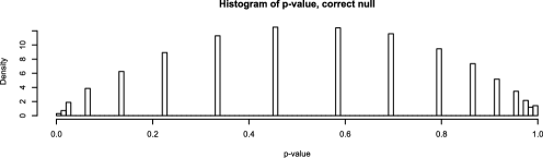
Figure 1: $p$-values $p_{i}=F_{i}(x_{i})$, where $x_{i}\sim F_{i}=\operatorname{Poisson}(10)$.

2.3 Randomized $p$-values

One way to fix this problem is to randomize the $p$-values to make them continuous. Randomized $p$-values are familiar from classical hypothesis testing [Lehmann and Romano (2005)], and have long been used in the forecasting literature to assess predictive distributions for discrete data [Brockwell (2007), Czado, Gneiting and Held (2009), Kulinskaya and Lewin (2009)] recently used randomized $p$-values to construct versions of the Bonferroni and Benjamini–Hochberg multiple testing procedures for discrete data. Their approach, however, has drawbacks that make it unsuitable for our purposes. It offers no way to check the nulls, to fit an empirical null, or to use existing continuous $\mathit{fdr}$ methods. More seriously, it produces a “probability of rejection” for each case, not a false discovery rate, and is too computationally expensive to apply to even moderately large data sets.

We propose using existing continuous false discovery rate methods on randomized $p$-values. Let

$$r_{i} = F_{i}^{-}(x_{i})+U_{i}\bigl{(}F(x_{i})-F_{i}^{-}(x_{i})\bigr{)}$$

$$= P_{F_{i}}(X<x_{i})+U_{i}P_{F_{i}}(X=x_{i}),$$

where $F_{i}^{-}=P(X_{i}<x_{i})$ denotes the left-limit function of the cdf $F_{i}$, $U_{i}$ are i.i.d. $\operatorname{Unif}(0,1)$ independent of all the $x_{i}$, and $P_{F_{i}}$ denotes probability under $X\sim F_{i}$. In other words, we use $r_{i}\sim\operatorname{Unif}(F_{i}^{-}(x_{i}),F_{i}(x_{i}))$ instead of $p_{i}=F_{i}(x_{i})$.

The key property of $r_{i}$ is that if our null distribution $F_{i}$ is correct, then $r_{i}\sim\operatorname{Unif}(0,1)$ under the null. This modification (of $p_{i}$ to $r_{i}$) allows us to apply continuous $\mathit{fdr}$ methods to the $r_{i}$. Theorem 2.1 makes this property more precise: The closer $r_{i}$ is to uniform, the closer our true null distribution is to the assumed null $F_{i}$, and vice versa. The theorem (proved in the Appendix) also holds for the nonrandom discrete $p$-value functions proposed by Czado, Gneiting and Held (2009), which can be used instead of our randomized $p$-values in everything that follows.

Theorem 2.1

Let $x$ be a discrete random variable, $F$ be our predicted distribution for $x$, and $G$ be the true distribution of $x$. Let $r=F^{-}(x)+U(F(x)-F^{-}(x))$ be our constructed randomized $p$-value, with density $h(r)$, cdf $H(r)$, and let $h_{\mathrm{unif}}(t)=1$, $H_{\mathrm{unif}}(t)=t$ be the uniform density and cdf.

Then

$$D_{\mathrm{KL}}(H_{\mathrm{unif}}\|H) = D_{\mathrm{KL}}(G\|F),$$

$$D_{\mathrm{KL}}(H\|H_{\mathrm{unif}}) = D_{\mathrm{KL}}(F\|G),$$

$$\sup_{r\in[0,1]}|H(r)-H_{\mathrm{unif}}(r)| = \sup_{x}|F(x)-G(x)|,$$

where for two distribution functions $P$ and $Q$, $D_{\mathrm{KL}}(P\|Q)=\int\log(\frac{dP}{dQ})\,dP$ is the Kullback–Liebler divergence. In particular, $r\sim\operatorname{Unif}(0,1)$ if and only if $F=G$.

Theorem 2.1 says that if our null distribution $F_{i}$ is correct, then $r_{i}$ is uniform under the null. Moreover, if our null distribution is close to the true null in the Kullback–Liebler or Kolmogorov distance, then $r$ is close to uniform in the same sense under the null. Consider our previous example, where $x_{i}\sim\operatorname{Poisson}(10)$. Figure 2 shows that $r_{i}$ are uniform if we use the correct $\operatorname{Poisson}(10)$ null. If we use the wrong null, $\operatorname{Poisson}(5)$, then $r_{i}$ are clearly not uniform. The distance between the distribution of $r_{i}$ and the uniform distribution is exactly the distance between the assumed null $\operatorname{Poisson}(5)$ and the correct null $\operatorname{Poisson}(10)$.

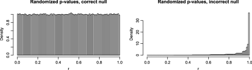
Figure 2: Histograms of randomized $p$-values $r_{i}$ under the correct $\operatorname{Poisson}(10)$ null (left) and the incorrect $\operatorname{Poisson}(5)$ null (right). The Kolmogorov distance between the distribution of $r_{i}$ under the incorrect null and the uniform distribution is $0.6464$, exactly the Kolmogorov distance between $\operatorname{Poisson}(5)$ and $\operatorname{Poisson}(10)$. The distance from the empirical cdf of the realized $r_{i}$ in the histogram to the uniform distribution is $0.6465$, which is different only because of the randomness in $x$ and $r$.

Theorem 2.1 lets us check our null distributions, fit empirical null distributions, and estimate false discovery rates using tools developed for continuous data. Consider the first problem, checking the null distributions. We know that most $x_{i}$ each come from their null distribution, and that if we have assumed the correct null distributions, $r_{i}\sim\operatorname{Unif}(0,1)$ under the null. We can check for systematic departures from the assumed null distributions by assessing the $r_{i}$ histogram just as we checked our nulls using the $p$-value histogram for continuous data, using any model assessment tool from the continuous $\mathit{fdr}$ literature.

Next, consider estimating an empirical null distribution. We can use continuous empirical null methods to fit a null distribution $H$ to $r_{i}$. Just as in the continuous case, we can then use $H$ to fix our null distributions, changing $F_{i}$ to $\tilde{F}_{i}=H\circ F_{i}$, and substituting $\tilde{F}$ in place of $F$ in (2.3) to make new randomized $p$-values $\tilde{r}_{i}$. Theorem 2.1 says that if $\tilde{r}_{i}$ is approximately uniform, $\tilde{F}_{i}$ is close to the true null distribution.

Finally, consider estimating $\mathit{fdr}$. Using Bayes’ rule, we can write

$$\mathit{fdr}(x_{i})=\frac{P(H_{i0})P_{\mathrm{null}}(x_{i})}{P_{\mathrm{marg}}(x_{i})},$$

where $P_{\mathrm{null}}$ and $P_{\mathrm{marg}}$ are the null and marginal distributions of $x_{i}$. Rewriting in terms of $\tilde{r}_{i}$, this is,

$$\mathit{fdr}(x_{i})=\frac{P(H_{i0})P_{\mathrm{null}}(\tilde{r}_{i}\in[\tilde{F}_{i}^{-}(x_{i}),\tilde{F}_{i}(x_{i})])}{P_{\mathrm{marg}}(\tilde{r}_{i}\in[\tilde{F}_{i}^{-}(x_{i}),\tilde{F}_{i}(x_{i})])}.$$ (3)

As before, we bound $P(H_{i0})$ by $1$, and since $\tilde{r}_{i}$ are uniform under the null,

$$P_{\mathrm{null}}\bigl{(}\tilde{r}_{i}\in[\tilde{F}_{i}^{-}(x_{i}),\tilde{F}_{i}(x_{i})]\bigr{)}=\tilde{F}_{i}(x_{i})-\tilde{F}_{i}^{-}(x_{i}).$$

We can model the $\tilde{r}_{i}$ as having approximately the same marginal distribution since they are all $\operatorname{Unif}(0,1)$ under the assumed null distribution. This lets us use the distribution of $\tilde{r}_{i}$ to estimate the marginal probability in the denominator of (3). Substituting these three values into (3) gives us an estimated false discovery rate. Randomization thus lets us translate the three key steps in a continuous $\mathit{fdr}$ analysis to the discrete setting.

It is important to note that although we use randomized $p$-values, the variability in the randomization does not significantly affect our final $\mathit{fdr}$ estimates. Given $\tilde{F}$, the false discovery rate in (3) is a deterministic function of the data $x$, so the randomization step affects our $\mathit{fdr}$ estimate only through the estimated empirical null $\tilde{F}$ and the marginal distribution of $\tilde{r}_{i}$. These quantities depend on the empirical distribution of all or most of the $\tilde{r}_{i}$’s, and do not depend strongly on any individual $\tilde{r}_{i}$. For large $P$, the empirical distribution of $\tilde{r}_{i}$ will be close to its true distribution, which is a deterministic function of the $x_{i}$’s. Thus, for large $P$, the variability in the randomization will have little effect on our $\mathit{fdr}$ estimates. For small $P$, if the extra variability from randomization is a concern, we can substitute the nonrandom $p$-value functions proposed by Czado, Gneiting and Held (2009) with essentially no change to our analysis.

3 Modeling sequencing error rates

In this section, we turn to the application of detecting DNA mutations and present an empirical Bayes model for sequencing error rates. Mutations appear in the data as unusually high observed error rates, so detecting mutations accurately requires understanding the normal variation in error rates. We begin by describing two example data sets and summarizing the existing approaches. Then, we describe a hierarchical model for observed error rates that accounts for sample effects, genome position, and finite depth. Our model shares information across positions and samples to estimate error rates and quantify their variability.

3.1 Example data sets: Virus and tumor

Our first example is motivated by the problem of detecting rare mutations in virus and microbial samples. Deep, targeted sequencing has been used to identify mutations that are carried by a very small proportion of individuals in the sample. Detecting these rare mutations is important, because they represent quasispecies that may expand after vaccine treatment. We use the synthetic DNA admixture data from Flaherty et al. (2012), in which a reference and a mutant version of a synthetic 281 base sequence are mixed at varying ratios. The mutant differs from the reference at 14 known positions. This data set contains six samples, 3 of which are 100$\%$ reference, the other 3 contain a 0.1$\%$ mixture of the mutant sequence. These samples were sequenced on an Illumina GAIIx platform. The reads were then aligned to the reference sequence, yielding nonreference counts (“errors”) $x_{ij}$ and depth $N_{ij}$ for each position ($i=1,\ldots,P=281$, $j=1,\ldots,S=6$) [see Flaherty et al. (2012) for more details]. Our goal is to find the mutations, which appear in the data as unusually large error rates $x_{ij}/N_{ij}$.

Our second example is a comparison of normal and tumor tissue in $S=28$ lymphoma patients, plus tissue from one healthy individual sequenced twice as a control. A set of regions containing a total of $P=309\mbox{,}474$ genome positions was extracted from each sample and sequenced on the Illumina GAIIx platform, yielding nonreference counts $x_{ij},y_{ij}$ and depths $N_{ij},M_{ij}$ for the normal and tumor tissues. Our goal is to find positions that show biologically interesting differences between the normal and tumor samples, such as positions that are mutated in the tumor or variant positions in the normal that have seen a loss of heterozygosity. These appear in the data as significant differences between the error rates $x_{ij}/N_{ij}$ and $y_{ij}/M_{ij}$.

The two detection problems pose different challenges. Since virus genomes are short, they can be sequenced to uniformly high depth. For example, the synthetic virus data from Flaherty et al. (2012) has depth in the hundreds of thousands. Human tissue, however, is usually sequenced to a lower, more variable depth. The tumor data has a median depth of $171$, but the depth varies over five orders of magnitude, from $0$ to over $100\mbox{,}000$. Discreteness is thus a more serious problem for the tumor application than it is for the virus application. The tumor data also exhibits much more variation in error rates, from less than $0.1\%$ to over $20\%$, because the human genome is harder to target and map.

Analyzing the virus data is difficult primarily because we are interested in very rare mutations. A mutation carried by $0.1\%$ of the viruses may be biologically interesting, but one carried by $0.1\%$ of the tumor cells is typically less interesting, since biologists usually are interested in mutations present in a substantial fraction of the tumor cells. Despite the high sequencing depth, it is difficult to detect such a small change in base proportions using discrete counts.

3.2 Existing approaches

Most current methods for variant detection in sequencing data are designed to analyze samples of DNA from pure, possibly diploid, cells. In pure diploid samples, variants are present at levels of either $50\%$ or $100\%$ of the sample, and are thus much easier to detect than variants in mixed samples, where they may be present at continuous fractions. Nearly all existing methods, including the widely used methods of Li, Ruan and Durbin (2008) and McKenna et al. (2010), rely on sequencing quality scores from the Illumina platform and mapping quality metrics to identify and filter out high-error positions. Storing and processing these quality metrics is computationally intensive, and methods utilizing these metrics are not portable across experimental platforms.

Muralidharan et al. (2012) proposed a method to detect single nucleotide variants in normal diploid DNA. Their method uses a mixture model with mixture components corresponding to different possible genotypes, and pools data across samples to estimate the null distribution of sequencing errors at each position. They showed that this approach, which avoids using quality metrics, outperforms existing quality metric based approaches.

A different approach to variant detection was proposed by Natsoulis et al. (2011), who use techniques based on domain knowledge, such as repeat masking (see Section 4.2) and double-strand confirmation (evidence for the variant must be present in both the forward and reverse reads covering the position) to identify high-error positions and eliminate false calls. This method can also be used to call mutations in tumors using matched normal samples.

Although most current methods for variant detection are designed for pure diploid samples, a few methods for detecting rare variants in virus data have recently been proposed. Hedskog et al. (2010) find simple upper confidence limits for the error rate and use them to test for variants. Flaherty et al. (2012) use a Beta-Binomial model, that is, less conservative but much more powerful. Their model for sequencing error rates is similar in form to ours, but uses a Beta distribution for error rates that we find does not fit the data. Hedskog et al. (2010) and Flaherty et al. (2012) also do not account for the effects of sample preparation on the error rates. Finally, both papers simply use a Bonferroni bound to avoid multiple testing concerns. This is reasonable since the data they analyze have only a few hundred positions, but it makes their methods inapplicable to large genomic regions where multiple testing is a more serious problem.

3.3 Sequencing error rate variation

Sequencing error rates show three types of variation. The first type of error rate variation comes from finite depth. Consider a nonmutated position, where all nonreference counts are truly errors. Given the depth and an error rate, we can model the nonreference counts as binomial,

$$x\sim\operatorname{Binomial}(N,p).$$ (4)

Because $N$ is finite, the observed error rate $x/N$ will vary around the true error rate $p$. This type of variation is easily handled by the binomial model.

Figure 3: Observed error rates $\operatorname{logit}(x/N)$ for two reference samples in the virus data. The solid green line is the $x=y$ diagonal. The error rates for the second sample are slightly but significantly biased upward. The dashed blue line shows the diagonal shifted to account for this bias.

The second type of variation is positional: as shown by Muralidharan et al. (2012) and Flaherty et al. (2012), different positions in the genome have different error rates. This means that each position has its own error rate $p$ in our binomial model (4). Suppose we have extremely large depth, so that the binomial variation in the observed error rate $x/N$ is negligible. A large observed error rate at a given position is still not enough to report a mutation, because that position may simply be noisy. We can account for the positional variation in error rates by aggregating data across samples to estimate the baseline sequencing error $p$ at each position.

The last type of variation is variation across samples. Small differences in sample preparation and sequencing, such as the sample’s lane assignment on the Illumina chip, can create differences in the sequencing error rate at each position, even when the sample contains no mutations. For example, suppose that we have extremely large depth, that we have estimated the positional error rate $p$ perfectly, and that we observe an error rate $x/N$, that is, higher than $p$. We still cannot conclude that the position is mutated, because the difference between $x/N$ and $p$ may be due to sample preparation. We can account for cross-sample variation by aggregating data across positions to estimate sample effects.

Figure 3 illustrates these three sources of variation. It plots, on the logit scale, observed error rates $x/N$ for two reference samples from the synthetic data of Flaherty et al. (2012). Each point in the plot represents a position. There are no mutant positions, so all points represent null observed error rates. The figure shows that error rates in the two samples are highly correlated and depend strongly on genome position. The binomial variation due to finite depth causes some of the spread around the diagonal. Sample variation also causes spread around the diagonal, as well as a systematic bias-error rates for the second sample are slightly but significantly higher than error rates in the first. These two samples were actually sequenced in the same lane; we observed stronger sample effects when comparing data from different lanes. We also saw similar behavior on the tumor data.

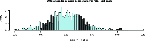
Figure 4: Differences between observed error rate $x/N$ and positional error rate $\mu$ for the three reference samples, on the logit scale. The mean error rate $\mu$ was estimated by averaging $\operatorname{logit}(x/N)$ for each position over the reference samples.

3.4 Modeling the variation

Figure 3 also suggests a model for sequencing error rates—when plotted on the logit scale, the error rates are dispersed evenly around a shifted diagonal. Figure 4 shows that the dispersion in error rates is roughly normal. Accordingly, we can model the logit sequencing error rate in each sample as a sum of a positional error rate, sample bias, and normally distributed sample noise. Given the error rate, we observe binomial counts. This model makes sense biologically: sample preparation for these two data sets includes PCR amplification, an exponential process, so it is plausible that differences in sample preparation produce additive effects on the logit scale.

This formulation yields the following hierarchical model for the unmatched mutation detection problem such as in the virus application:

$$\operatorname{logit}p_{ij} \sim \mathcal{N}(\operatorname{logit}\mu_{i}+\delta_{j},\sigma_{j}^{2}),$$

$$x_{ij}|p_{ij} \sim \operatorname{Binomial}(N_{ij},p_{ij}),$$

where $\mu_{i}$ is the positional error rate, $\delta_{j}$ is a sample-specific error rate bias (constant across positions), and $\sigma_{j}$ measures the sample specific noise in error rates. Fitting $\mu$, $\delta$, and $\sigma$ provides information on the positional error rates, sample biases, and cross-sample variability in our data.

This model allows us to test whether an observed error rate is unusual enough to be a mutation. For example, consider applying the model to the virus data. Once we fit the parameters, as described in Section 3.4.1, the model gives a null distribution for the observed error rate at each position. We can then compare the observed error rates for each position in a clinical sample to its null distribution and use the false discovery rate methods from Section 2 to find mutated positions.

Next, consider tumor data with matched normals. We model the normal tissue error rates as in (3.4), and introduce extra parameters to account for additional error rate variation between normal and tumor tissue from the same patient:

$$\operatorname{logit}p_{ij} \sim \mathcal{N}(\operatorname{logit}\mu_{i}+\delta_{j},\sigma_{j}^{2}),$$

$$\operatorname{logit}q_{ij}|p_{ij} \sim \mathcal{N}(\operatorname{logit}p_{ij}+\eta_{j},\tau_{j}^{2}),$$

$$x_{ij}|p_{ij},q_{ij} \sim \operatorname{Binomial}(N_{ij},p_{ij}),$$

$$y_{ij}|p_{ij},q_{ij} \sim \operatorname{Binomial}(N_{ij},q_{ij}),$$

where $p_{ij}$, $q_{ij}$ are the normal and tumor error rates, respectively; $\delta_{j},\eta_{j}$ are sample effects, $\sigma_{j}$ is the noise variance for the normal tissue, and $\tau_{j}$ is the noise variance for the difference between tumor and normal tissue. After fitting the parameters as described in Section 3.4.1, we use this model to find the conditional null distribution for the tumor error rates, given the observed normal error rates. That is, we use the model to find null distributions for

$$\frac{y_{ij}}{M_{ij}}\bigg{|}\frac{x_{ij}}{N_{ij}},$$

and then use the false discovery rate approach in Section 2 to find mutated positions.

The logit-normal model naturally handles the discreteness and wide range of depths in our data. It separates the observed error rate variation into depth, positional variation, and sample effects, and combines the different sources of variation to give the appropriate null distribution in each case.

3.4.1 Fitting

The best way to fit our model will depend on the data set, so we will discuss the fitting in only general terms.

Estimating $\mu,\delta$, and $\eta$ is usually straightforward. For example, in the virus data set, we use the median of the observed error rates for each position over all of the reference samples to estimate $\mu$, then estimate $\delta$ using all of the positions in each sample,

$$\hat{\delta}_{j}=\operatorname{median}\biggl{(}\operatorname{logit}\frac{x_{ij}}{N_{ij}}-\operatorname{logit}\hat{\mu}_{i}\biggr{)}.$$

Similar ideas can also be applied to estimate these parameters for the tumor data.

Estimating the sample error rate variances $\sigma$ and $\tau$ can be more difficult. The simplest and fastest approach is to use the method of moments as an approximate version of maximum likelihood. This works well if depths are large, as in the virus data. If depths are small, as in the tumor data, the method of moments works badly and it is better to use the maximum likelihood.

The tumor data also has extra sources of variability, which we discuss briefly to illustrate how our method can be adapted to the specific characteristics of a data set. Because of genetic variation between people, not all normal samples have the same base at each position. For example, at single nucleotide polymorphic positions (SNPs), heterozygous samples have an observed “error rate” close to $0.5$ against the reference genome, while homozygous samples have an observed error rate close to $0$. We account for SNP positions by using a simple mixture model to genotype the samples and estimating $\mu_{i}$ separately for each genotype. We also increase $\sigma_{j}^{2}$ for positions with multiple genotypes to account for the extra uncertainty due to possibly incorrect genotyping.

Another source of extra variability comes from the technology used to generate our data set: The 309,474 genome positions are regions of the genome that have been targeted by primers and amplified. We observe empirically that regions treated with some primers have more variable error rates across samples. These regions can be identified using extra data generated by the sequencer. We account for this extra variability by fitting different error variances $\sigma_{j}$ and $\tau_{j}$ for each genomic region, and using a high quantile of the region-wise variabilities as our $\sigma_{j}$.

The logit-normal prior for $p$ makes it difficult to calculate the marginal distributions of counts, find predictive distributions, and fit $\sigma,\tau$ by maximum likelihood. We approximate the logit-normal distribution with a Beta distribution. If

$$p\sim\operatorname{Beta}\biggl{(}\frac{1}{\sigma^{2}(1-\mu)},\frac{1}{\sigma^{2}\mu}\biggr{)},$$

then it is easy to show using Stirling’s formula that $\operatorname{logit}p$ has approximate mean $\operatorname{logit}\mu$, variance $\sigma^{2}$, skewness

$$\sigma\bigl{(}\mu^{3}-(1-\mu)^{3}\bigr{)},$$

and excess kurtosis

$$2\sigma^{2}\bigl{(}\mu^{4}+(1-\mu)^{4}\bigr{)}.$$

If $\sigma$ is small and $\mu$ is close to $0$ or $1$, as they are in our data, then $\operatorname{logit}p$ is approximately $\mathcal{N}(\operatorname{logit}\mu,\sigma^{2})$. This Beta approximation makes it much easier to calculate marginal and posterior distributions.

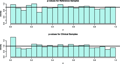
Figure 5: Histogram of $p$-values for the virus data, reference samples (top plot) and clinical samples (bottom plot).

Table 1: Detection results on clinical samples of the synthetic virus data

	Our method,	Our method,
	$\bolds{\hat{\mathit{fdr}}\leq 0.1}$	$\bolds{\hat{\mathit{fdr}}\leq 0.01}$	Flaherty et al.
True positives (of 42)	420	3900	420
False positives	.1	00	100
Power	100%	93%	100%
False positive rate	0000.2.32%	00%	000.19.23%

4 Results

4.1 Virus data

We first tested our method by applying it to the virus data, described in Section 3.1. In this synthetic data, we know the locations of the 14 variant positions, and we know that the mutant base is present in $0.1\%$ of the viruses in each case. We did not use any information about the mutations’ location or prevalence when fitting our model. Thus, we can use this data to evaluate our method’s power and specificity.

Our model fits the data reasonably well. Figure 5 shows the $p$-values histograms for the reference and clinical samples; randomization is unnecessary since the depth is so high (the median depth is $775\mbox{,}681$, and $95\%$ of positions have depth between $271\mbox{,}192$ and $1\mbox{,}689\mbox{,}977$). The $p$-values are fairly uniform for the reference samples, and also uniform in the clinical samples except for a spike near $0$ that indicates that some positions are truly nonnull. Since our null distributions fit the data accurately enough, we did not need to estimate an empirical null. We used the log-spline $\mathit{fdr}$ estimation method proposed by Efron (2004) to estimate the false discovery rate $\hat{\mathit{fdr}}_{ij}$ for each position in each sample. Finally, we declared any position with $\hat{\mathit{fdr}}$ less than a given threshold to be a mutation.

Table 1 compares our results to the method of Flaherty et al. (2012). Our method produces fewer false discoveries while maintaining excellent power. If we use an $\hat{\mathit{fdr}}$ threshold of $10\%$, our method detects all $42$ mutations (14 in each clinical sample) and makes $1$ false discovery, for a false positive rate of $2.3\%$. A more stringent $\mathit{fdr}$ threshold of $1\%$ eliminates all false discoveries, at the cost of missing $3$ mutations. Our method’s high power and low false discovery rate is especially notable given that the mutation is only present at $0.1\%$ within the sample.

4.2 Tumor data

Next, we applied our method to the tumor data, also described in Section 3.1. Our model fits the data relatively well, but not as accurately as it fits the virus data. We can assess the model by examining the last sample pair, which actually consists of a healthy person’s normal tissue that was sequenced twice as though it were normal and tumor tissue.

Figure 6 shows the histogram of randomized and unrandomized $p$-values for the last sample pair. The randomized $p$-values $r_{ij}$ are uniform through most of the unit interval, indicating that most of our fitted null distributions are close to the true null distributions. In contrast, the unrandomized $p$-value histogram tells us next to nothing about our null distributions.

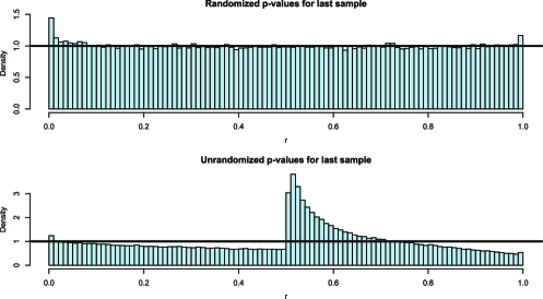
Figure 6: Randomized $r_{ij}$ (top plot) and unrandomized $p_{ij}$ (bottom plot) values for the last normal tumor pair (actually the same normal tissue sequenced twice).

Our null distributions do not give a perfect fit: the $r_{ij}$ appear to be enriched near $0$ and $1$, so if we thought the null were uniform, our false discovery rates would be misleadingly small near $0$ and $1$. Empirical nulls are not very helpful here, because they are fit to the center of the distribution rather than the tails. Inspecting the sample reveals that the null distribution is enriched near $0$ and $1$ because the error rates $p$ and $q$ are more variable very close to $0$ and $1$ than our normal model predicts. We will discuss this issue a bit more later.

Although our null distributions are mostly correct for the last sample, they are not as good on some other samples. Figure 7 shows the randomized $p$-value histogram for the seventh sample pair, which shows the most deviation from uniformity. The underdispersion in Figure 7 means that our null distributions are systematically too wide on that sample.

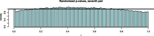
Figure 7: Randomized $p$-values $r_{i}$ for the seventh normal tumor pair. This sample had the least uniform $r_{i}$.

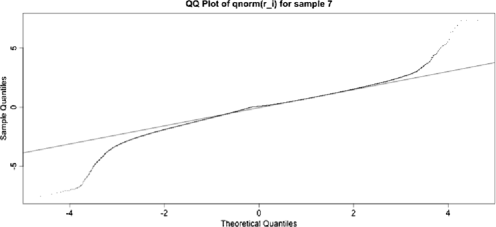
Figure 8: Normal QQ plot of $z_{ij}=\Phi^{-1}(r_{ij})$ for sample $7$.

We fit empirical nulls to correct our null distributions. Figure 8 shows a normal quantile–quantile plot of randomized $p$-values for sample $7$, transformed to the normal scale by $z_{ij}=\Phi^{-1}(r_{ij})$. The QQ plot is straight through the bulk of the data, indicating that our null can be corrected by centering and scaling on the normal scale. Our corrected null will still be too light-tailed in the far tails, but, as for the last sample, these points correspond to very small changes in error rate very close to $0$ and $1$, which we will discuss later. Accordingly, we used the median and a robust estimator of scale [$S_{n}$, described by Rousseeuw and Croux (1993)] on $z_{ij}$ to estimate a location and scale for our empirical null in each sample. Figure 9 shows that this yielded much more uniform randomized $p$-values.

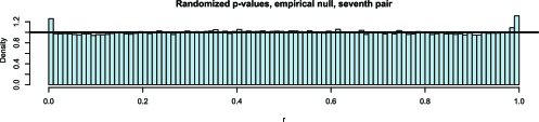
Figure 9: Empirical null randomized $p$-values $\tilde{r}_{i}$ for the seventh normal tumor pair. The empirical null yields much more uniform $p$-values (compare to Figure 7).

Finally, we estimated the density of the empirical null adjusted randomized $p$-values using a log-spline. We then estimated the $\mathit{fdr}$. To ease computation, we approximated the $\mathit{fdr}$ expression in equation (3). Instead of estimating

$$P_{\mathrm{marg}}\bigl{(}\tilde{r}_{i}\in[\tilde{F}_{i}^{-}(x_{i}),\tilde{F}_{i}(x_{i})]\bigr{)},$$

we fit $f_{\mathrm{marg}}$ and used the approximation

(6)

Substituting (LABEL:fmarg) into (3) yields an estimate of the false discovery rate $\hat{\mathit{fdr}}_{ij}$ for each position in each sample.

As mentioned, many positions had a low $\hat{\mathit{fdr}}$ while being biologically uninteresting due to the heavier tail of the null $p$-value distribution around 0 and 1. Our model looks at differences between normal and tumor error rates on the logit scale, which exaggerates differences near $0$ and $1$; for example, on the logit scale, $0.001$ and $0.003$ are as far from each other as $0.5$ and $0.75$. Such small changes near $0$ and $1$ are also more likely to be false positives, since null error rates are more variable very near $0$ and $1$ than our model predicts. Even if they were real, mutations present at such small fractions in tumor tissue are too rare to be biologically interesting. For most tumor analysis scenarios, we want to find mutations that are present in a fairly large fraction of the cells in the tumor tissue, with the prevalence threshold determined by the biologist.

To find such mutations, we estimated the change in error rate at each position for each sample using a very simple “spike and slab” model. We supposed that either the normal and tumor error rates were the same, or they were different, in which case we knew nothing about either. Under this model, the expected error rate difference given the data is

$$\Delta_{ij} = E(q_{ij}-p_{ij}|x,y)$$

$$= P(q_{ij}\neq p_{ij}|x,y)\biggl{(}\frac{y_{ij}}{M_{ij}}-\frac{x_{ij}}{N_{ij}}\biggr{)},$$

which we can estimate by

$$\hat{\Delta}_{ij}=\hat{\mathit{fdr}}_{ij}\biggl{(}\frac{y_{ij}}{M_{ij}}-\frac{x_{ij}}{N_{ij}}\biggr{)}.$$

We required a position to have a large $\hat{\Delta}$ ($|\hat{\Delta}|\geq 0.25$) as well as a low $\hat{\mathit{fdr}}$ $(\hat{\mathit{fdr}}\leq 0.1)$ to be called a biologically interesting mutation.

Thresholding for both false discovery rate and estimated effect size yielded 427 mutation calls on the clinical samples. Assessing these calls is difficult. Unlike for the synthetic data, we do not know which positions are truly mutated or null for the tumor data. Since all putative mutations in the tumor samples are new changes, and would be unique to each sample, we cannot assess our mutation calls using databases of known variants. Also, targeted deep resequencing is currently the best technology for variant detection, so, short of resequencing the entire genomic region at even higher depth, we cannot use some other gold-standard experimental method to validate our calls.

We therefore use a simple domain-knowledge based proxy, enrichment in repetitive regions, as a crude check that our method gives useful results. Repetitive regions are segments of DNA that repeat themselves with high sequence similarity at multiple places in the genome. They confuse the DNA targeting, extraction, and mapping steps in the experiment, and have been a major source of false calls for previous variant detection methods. Because of this, most existing variant detection methods use repeat detection algorithms to find repetitive regions, and then use the output of these algorithms to refine their calls. The most common approach has been to simply ignore calls in regions that are designated as repetitive, since otherwise the calls would be dominated by false calls in these regions.

Masking repetitive regions has some disadvantages. First, different repeat detection algorithms often disagree, so the choice of repeat detection method and associated parameters can substantially impact the final list of calls. Second, many functional areas of the genome, such as exons, contain repeated genetic material. For example, roughly $8.5\%$ of our tumor data, which consists almost entirely of exons, lie in repetitive regions (the exact percentage depends on the repeat detector and parameters used). If we simply ignore mutation calls in repetitive regions, we may miss important mutations in functional regions.

Our approach does not rely on any information about whether a position lies in a repetitive region. The high error rates in repetitive regions are reproducible across samples, and thus by modeling the error rate as a function of genome position, we can account for the higher error rates in repetitive regions without using any explicit information about repetitiveness.

Of the $427$ mutations found in the tumor data by our method, $95$ ($22.1\%$) lie in repetitive regions. In comparison, Natsoulis et al. (2011) make $1305$ calls before their final repeat masking step, $470$ ($36\%$) of which are in repetitive regions. Although our calls are somewhat enriched in repetitive regions, they are less enriched than the calls made by Natsoulis et al. (2011) before repeat masking, despite not using any domain knowledge explicitly. This is a rough indication that our positional error-rate model is estimating higher error rates in repetitive regions.

Our method makes more calls than Natsoulis et al. (2011) in low depth regions. We make a $233$ gain of allele calls, $47$ ($20.1\%$) of which are in repetitive regions. Of the $186$ calls we make outside of repetitive regions, $103$ are among the $165$ gain of allele calls made by Natsoulis et al. (2011). Nearly half of the $83$ calls made by our method outside repetitive regions and not made by Natsoulis et al. (2011) are in low depth regions of the genome. We would like to think that this indicates our method is able to achieve higher power in low depth regions by pooling data across samples to estimate the null distribution of the error rates. We cannot know the truth, however, without a rigorous validation experiment.

4.3 Summary

In this paper, we have shown that empirical Bayes ideas can be usefully applied to detect mutations in high throughput sequencing data from mixed DNA samples. We used a hierarchical model to account for different sources of variation in sequencing error rates. This model let us weigh the different sources against one another, and naturally accommodates the discreteness and depth variation in our data. We also adapted continuous $\mathit{fdr}$ methods to discrete data using a simple randomization scheme. Combining the new multiple testing methods with the empirical null distributions for sequencing error rates yielded a powerful, statistically sound way to detect mutations in mixed samples.

Appendix

We prove Theorem 2.1, which justifies the use of randomized $p$-values. From the construction of $r$, we have that

$$r|x\sim\operatorname{Unif}(F^{-}(x),F(x)).$$

Thus, the unconditional density of $r$ is

$$h(r)=\sum_{x}\frac{P_{G}(x)}{P_{F}(x)}I_{r\in[F^{-}(x),F(x)]},$$

where $P_{F}$ and $P_{G}$ denote probability under $F$ and $G$ respectively. This means that

$$D_{\mathrm{KL}}(H_{\mathrm{unif}}\|hH) = \int\log\biggl{(}\frac{h(r)}{h_{\mathrm{unif}}(r)}\biggr{)}h(r)\,dr$$

$$= \sum_{x}\int_{F^{-}(x)}^{F(x)}\frac{P_{G}(x)}{P_{F}(x)}\log\biggl{[}\frac{P_{G}(x)}{P_{F}(x)}\biggr{]}\,dr$$

$$= \sum_{x}P_{G}(x)\log\frac{P_{G}(x)}{P_{F}(x)}$$

$$= D_{\mathrm{KL}}(G\|F).$$

The other Kullback–Liebler equality is proved similarly.

For the Kolmogorov distance, note that the cdf of $r$, $H$, is piecewise linear, and the uniform cdf $H_{\mathrm{unif}}(r)=r$ is also linear. This means that $|H-H_{\mathrm{unif}}|$ reaches its maximum at one of the knots of $H$, and these are $0$, $1$, and $F(x)$ for all possible values of $x$. Since $H(0)=H_{\mathrm{unif}}(0)=0$ and $H(1)=H_{\mathrm{unif}}(1)=1$, the maximum has to occur at some $F(x)$. At these points, though,

$$H(F(x)) = P_{G}\bigl{(}r\leq F(x)\bigr{)}$$

$$= \sum_{x^{*}\leq x}\bigl{(}F(x^{*})-F^{-}(x^{*})\bigr{)}\frac{P_{G}(x^{*})}{P_{F}(x^{*})}$$

$$= G(x)$$

so

$$\sup_{r}|H(r)-H_{\mathrm{unif}}(r)| = \sup_{x}|H(F(x))-F(x)|$$

$$= \sup_{x}|G(x)-F(x)|.$$

References

- Benjamini and Hochberg (1995) {barticle}[mr] \bauthor\bsnmBenjamini, \bfnmYoav\binitsY. and \bauthor\bsnmHochberg, \bfnmYosef\binitsY. (\byear1995). \btitleControlling the false discovery rate: A practical and powerful approach to multiple testing. \bjournalJ. Roy. Statist. Soc. Ser. B \bvolume57 \bpages289–300. \bidissn=0035-9246, mr=1325392 \bptokimsref \endbibitem
- Brockwell (2007) {barticle}[mr] \bauthor\bsnmBrockwell, \bfnmA. E.\binitsA. E. (\byear2007). \btitleUniversal residuals: A multivariate transformation. \bjournalStatist. Probab. Lett. \bvolume77 \bpages1473–1478. \biddoi=10.1016/j.spl.2007.02.008, issn=0167-7152, mr=2395595 \bptokimsref \endbibitem
- Czado, Gneiting and Held (2009) {barticle}[mr] \bauthor\bsnmCzado, \bfnmClaudia\binitsC., \bauthor\bsnmGneiting, \bfnmTilmann\binitsT. and \bauthor\bsnmHeld, \bfnmLeonhard\binitsL. (\byear2009). \btitlePredictive model assessment for count data. \bjournalBiometrics \bvolume65 \bpages1254–1261. \biddoi=10.1111/j.1541-0420.2009.01191.x, issn=0006-341X, mr=2756513 \bptokimsref \endbibitem
- Efron (2004) {barticle}[mr] \bauthor\bsnmEfron, \bfnmBradley\binitsB. (\byear2004). \btitleLarge-scale simultaneous hypothesis testing: The choice of a null hypothesis. \bjournalJ. Amer. Statist. Assoc. \bvolume99 \bpages96–104. \biddoi=10.1198/016214504000000089, issn=0162-1459, mr=2054289 \bptokimsref \endbibitem
- Efron et al. (2001) {barticle}[mr] \bauthor\bsnmEfron, \bfnmBradley\binitsB., \bauthor\bsnmTibshirani, \bfnmRobert\binitsR., \bauthor\bsnmStorey, \bfnmJohn D.\binitsJ. D. and \bauthor\bsnmTusher, \bfnmVirginia\binitsV. (\byear2001). \btitleEmpirical Bayes analysis of a microarray experiment. \bjournalJ. Amer. Statist. Assoc. \bvolume96 \bpages1151–1160. \biddoi=10.1198/016214501753382129, issn=0162-1459, mr=1946571 \bptokimsref \endbibitem
- Flaherty et al. (2012) {bmisc}[author] \bauthor\bsnmFlaherty, \bfnmPatrick\binitsP., \bauthor\bsnmNatsoulis, \bfnmGeorges\binitsG., \bauthor\bsnmMuralidharan, \bfnmOmkar\binitsO., \bauthor\bsnmBuenrostro, \bfnmJason\binitsJ., \bauthor\bsnmBell, \bfnmJohn\binitsJ., \bauthor\bsnmZhang, \bfnmNancy\binitsN. and \bauthor\bsnmJi, \bfnmHanlee\binitsH. (\byear2012). \bhowpublishedUltrasensitive detection of rare mutations using next-generation targeted resequencing. Nucleic Acids Res. 40 (electronic). \bptokimsref \endbibitem
- Gneiting, Balabdaoui and Raftery (2007) {barticle}[mr] \bauthor\bsnmGneiting, \bfnmTilmann\binitsT., \bauthor\bsnmBalabdaoui, \bfnmFadoua\binitsF. and \bauthor\bsnmRaftery, \bfnmAdrian E.\binitsA. E. (\byear2007). \btitleProbabilistic forecasts, calibration and sharpness. \bjournalJ. R. Stat. Soc. Ser. B Stat. Methodol. \bvolume69 \bpages243–268. \biddoi=10.1111/j.1467-9868.2007.00587.x, issn=1369-7412, mr=2325275 \bptokimsref \endbibitem
- Hedskog et al. (2010) {barticle}[pbm] \bauthor\bsnmHedskog, \bfnmCharlotte\binitsC., \bauthor\bsnmMild, \bfnmMattias\binitsM., \bauthor\bsnmJernberg, \bfnmJohanna\binitsJ., \bauthor\bsnmSherwood, \bfnmEllen\binitsE., \bauthor\bsnmBratt, \bfnmGöran\binitsG., \bauthor\bsnmLeitner, \bfnmThomas\binitsT., \bauthor\bsnmLundeberg, \bfnmJoakim\binitsJ., \bauthor\bsnmAndersson, \bfnmBjörn\binitsB. and \bauthor\bsnmAlbert, \bfnmJan\binitsJ. (\byear2010). \btitleDynamics of HIV-1 quasispecies during antiviral treatment dissected using ultra-deep pyrosequencing. \bjournalPLoS ONE \bvolume5 \bpagese11345. \biddoi=10.1371/journal.pone.0011345, issn=1932-6203, pmcid=2898805, pmid=20628644 \bptokimsref \endbibitem
- Kulinskaya and Lewin (2009) {barticle}[mr] \bauthor\bsnmKulinskaya, \bfnmElena\binitsE. and \bauthor\bsnmLewin, \bfnmAlex\binitsA. (\byear2009). \btitleOn fuzzy familywise error rate and false discovery rate procedures for discrete distributions. \bjournalBiometrika \bvolume96 \bpages201–211. \biddoi=10.1093/biomet/asn061, issn=0006-3444, mr=2482145 \bptokimsref \endbibitem
- Lehmann and Romano (2005) {bbook}[mr] \bauthor\bsnmLehmann, \bfnmE. L.\binitsE. L. and \bauthor\bsnmRomano, \bfnmJoseph P.\binitsJ. P. (\byear2005). \btitleTesting Statistical Hypotheses, \bedition3rd ed. \bpublisherSpringer, \baddressNew York. \bidmr=2135927 \bptokimsref \endbibitem
- Li, Ruan and Durbin (2008) {barticle}[pbm] \bauthor\bsnmLi, \bfnmHeng\binitsH., \bauthor\bsnmRuan, \bfnmJue\binitsJ. and \bauthor\bsnmDurbin, \bfnmRichard\binitsR. (\byear2008). \btitleMapping short DNA sequencing reads and calling variants using mapping quality scores. \bjournalGenome Res. \bvolume18 \bpages1851–1858. \biddoi=10.1101/gr.078212.108, issn=1088-9051, pii=gr.078212.108, pmcid=2577856, pmid=18714091 \bptokimsref \endbibitem
- McKenna et al. (2010) {barticle}[pbm] \bauthor\bsnmMcKenna, \bfnmAaron\binitsA., \bauthor\bsnmHanna, \bfnmMatthew\binitsM., \bauthor\bsnmBanks, \bfnmEric\binitsE., \bauthor\bsnmSivachenko, \bfnmAndrey\binitsA., \bauthor\bsnmCibulskis, \bfnmKristian\binitsK., \bauthor\bsnmKernytsky, \bfnmAndrew\binitsA., \bauthor\bsnmGarimella, \bfnmKiran\binitsK., \bauthor\bsnmAltshuler, \bfnmDavid\binitsD., \bauthor\bsnmGabriel, \bfnmStacey\binitsS., \bauthor\bsnmDaly, \bfnmMark\binitsM. and \bauthor\bsnmDePristo, \bfnmMark A.\binitsM. A. (\byear2010). \btitleThe genome analysis toolkit: A MapReduce framework for analyzing next-generation DNA sequencing data. \bjournalGenome Res. \bvolume20 \bpages1297–1303. \biddoi=10.1101/gr.107524.110, issn=1549-5469, pii=gr.107524.110, pmcid=2928508, pmid=20644199 \bptokimsref \endbibitem