A two-way regularization method for MEG source reconstruction

Abstract

The MEG inverse problem refers to the reconstruction of the neural activity of the brain from magnetoencephalography (MEG) measurements. We propose a two-way regularization (TWR) method to solve the MEG inverse problem under the assumptions that only a small number of locations in space are responsible for the measured signals (focality), and each source time course is smooth in time (smoothness). The focality and smoothness of the reconstructed signals are ensured respectively by imposing a sparsity-inducing penalty and a roughness penalty in the data fitting criterion. A two-stage algorithm is developed for fast computation, where a raw estimate of the source time course is obtained in the first stage and then refined in the second stage by the two-way regularization. The proposed method is shown to be effective on both synthetic and real-world examples.

, ,
and au1Supported in part by the University of Houston New Faculty Research Program. au2Supported in part by NCI (CA57030), NSF (DMS-09-07170, DMS-10-07618) and King Abdullah University of Science and Technology (KUS-CI-016-04). au3Supported in part by NIDA (1 RC1 DA029425-01) and NSF (CMMI-0800575, DMS-11-06912).

1 Introduction

Magnetoencephalography (MEG) is a noninvasive neurophysiological technique that measures the magnetic field generated by neural activity of the brain using a collection of sensors outside the scalp [Papanicolaou (1995)]. When information is being processed at some regions of the brain, small currents will flow in the neural system, producing a small electric field, which in turn produces an orthogonally oriented small magnetic field according to Maxwell’s Equations. The MEG inverse problem refers to recovering neural activity by means of measurements of the magnetic field. The neural activities are usually represented by magnetic dipoles, which are closed circulations of electric currents, that is, loops with some constant current flowing through. Each dipole has a position, an orientation, and a magnitude. The inverse problem then becomes determining the position, orientation, and magnitude (or amplitude) of the dipoles.

One challenge of the MEG inverse problem is that it does not have a unique solution and so it is ill-posed [von Helmholtz (1853); Nunez (1981); Sarvas (1987)]. As early as in the 19th century, von Helmholtz demonstrated theoretically that general inverse problems, such as those aiming at identifying the sources of electromagnetic fields outside a volume conductor, have an infinite number of solutions [von Helmholtz (1853)]. Hence, to derive a practically meaningful solution from the infinitely many mathematically correct solutions, one has to introduce constraints to the solution and/or use prior knowledge about the brain activity.

Existing approaches for the MEG inverse problem can be grouped into two major classes that differ in how they impose constraints on the source signals. Within the first class, the dipole fitting [Scherg and Von Cramon (1986); Hämäläinen et al. (1993); Yamazaki et al. (2000); Jun et al. (2005)] and scanning methods [Sorrentino et al. (2009); Schmidt (1986); Mosher, Lewis and Leahy (1992); Veen and Buckley (1988); VanVeen et al. (1997); Dogandžić and Nehorai (2000)] assume that there exist a limited number of dipoles as point sources of the magnetic field in the brain. By constraining the number of sources, the locations of these dipoles are estimated by least squares fitting [Lu and Kaufman (2003)] or iterative computing [Baillet et al. (2001)]. Dipole orientations and amplitudes can be effectively estimated within these locations. However, estimating the source locations involves solving a difficult nonlinear optimization problem which has multiple local optima [Darvas et al. (2004)].

Our proposed method belongs to the second class, which contains various imaging methods. Different from the first class, imaging methods assume that there are a large number of potential dipole locations evenly distributed all over the cortex. By dividing the cortical region into a fine grid and attaching a dipole at each grid, imaging methods model the orientations and magnitudes for all the potential dipoles simultaneously. Dipoles with nonzero magnitudes are identified as the source dipoles. Imaging methods are based on the theory that the primary sources can be represented as linear combinations of neuron activities [Barlow (1994)]. One can express the inverse problem using a linear model

$${\mathbf{Y}}={\mathbf{X}}{\mathbf{B}}+{\mathbf{E}},$$ (1)

where ${\mathbf{Y}}$ is an $n\times s$ matrix containing MEG time courses measured by $n$ sensors at $s$ time points, recording the amplitudes of the magnetic field. Without loss of generality, it is assumed that the $s$ measurements for each time course are sampled at the same evenly-spaced time points. The known $n\times p$ design matrix ${\mathbf{X}}$ links the source signals to the sensor measurements, and is computed using a boundary element model prior to application of Model (1) [Mosher, Leahy and Lewis (1999)]. The $p\times s$ matrix ${\mathbf{B}}$ represents the unknown dipole activities in the form of $p$ unobservable source time courses. The $n\times s$ matrix ${\mathbf{E}}$ contains some additive noise. The amplitudes and orientations of the signal for each dipole at a time point can be decomposed into three components in the $x,~{}y,~{}z$ coordinate system. Therefore, $p$ represents the total number of the dipole components, and it is three times that of the number of grid cells. In a typical MEG study, $s$ is usually from a few hundred to a few thousand, $n$ is a few hundred, but $p$ is as large as over 10,000, and so $p\gg n$.

Defining the matrix Frobenius norm as $\|{\mathbf{B}}\|_{F}=\sqrt{\operatorname{tr}({\mathbf{B}}^{T}{\mathbf{B}})}$. To recover ${\mathbf{B}}$, one can solve a penalized least squares problem

$$\min_{{\mathbf{B}}}\{\|{\mathbf{Y}}-{\mathbf{X}}{\mathbf{B}}\|_{F}^{2}+\lambda\operatorname{pen}({\mathbf{B}})\},$$ (2)

where $\operatorname{pen}(\cdot)$ is a penalty function that promotes certain desirable properties on ${\mathbf{B}}$.

In the literature of MEG source reconstruction, spatial focality and temporal smoothness are two valid assumptions. That is, the source signals are smooth in time, and only a small number of compact areas are responsible for the recordings [Bolstad, Veen and Nowak (2009)]. Many of the imaging methods focus on either the first assumption or the second. Earlier methods using the smoothness assumption usually adopt the $L_{2}$-norm penalty, $\operatorname{pen}({\mathbf{B}})=\|{\mathbf{W}}{\mathbf{B}}\|_{F}^{2}$ for certain weighting matrix ${\mathbf{W}}$. The simplest such method is the minimum norm estimate (MNE) [Hämäläinen and Ilmoniemi (1994)] which uses ${\mathbf{W}}={\mathbf{I}}$. The LORETA methods [Pascual-Marqui, Michel and Lehmann (1994); Pascual-Marqui (2002)] set ${\mathbf{W}}$ to be the discrete spatial Laplacian operator. Two advantages of the $L_{2}$-penalty based methods are the computational efficiency and the less-spiky property in the time domain. Nevertheless, the $L_{2}$-penalty lowers the spatial resolution and causes the well-known “blurring effect” in the spatial domain. Utilizing the $L_{2}$-penalty, the FOCUSS method [Gorodnitsky and Rao (1997)] reduces the blurring effect by reinforcing the strong signals while weakening the weak ones using an iterative algorithm to update ${\mathbf{W}}$. However, it is noticed that FOCUSS is very sensitive to noise [Ou, Hämäläinen and Golland (2009)]. Many hierarchical Bayesian approaches induce the temporal smoothness by employing smoothing priors which penalize discontinuities [see, e.g., Baillet and Garnero (1997); Daunizeau et al. (2006); Nummenmaa et al. (2007a)].

An alternative penalty is the $L_{1}$-norm, $\operatorname{pen}({\mathbf{B}})=|{\mathbf{B}}|=\sum_{i}^{p}\sum_{j}^{s}|b_{ij}|$, which promotes the focality of the recovered signals. Related work includes the minimum current estimate (MCE) [Matsuura and Okabe (1995); Uutela, Hämäläinen and Somersalo (1999); Lin et al. (2006)] and the sparse source imaging method [Ding and He (2008)]. In contrast to the $L_{2}$-penalty, the $L_{1}$-penalty causes “spiky” discontinuities of the recovered signals in both temporal and spatial domains. Bayesian methods developed by Baillet and Garnero (1997), Friston et al. (2008), Nummenmaa et al. (2007b) take into account the spatial focality by employing anatomic sparse priors. However, these methods have similar problems as methods based on the $L_{1}$-penalty.

To prevent the spiky property from the $L_{1}$-penalty and the blurry property from the $L_{2}$-penalty, some $L_{l}$-norm methods with $0<l<1$ and $1<l<2$ have been introduced [Auranen et al. (2005); Jeffs, Leahy and Singh (1987)]. However, the optimization problems associated with $L_{l}$-penalties are more difficult to solve than with $L_{1}$ and $L_{2}$ penalties.

More recently, some spatio-temporal regularization methods have been proposed, which take into account both the smoothness and focality properties by combining basis representation with penalization. The $L_{1}L_{2}$-regularization discussed by Ou, Hämäläinen and Golland (2009) first projects ${\mathbf{B}}$ onto a temporal basis and then imposes the $L_{1}$-penalty on the spatial domain and the $L_{2}$-penalty on the temporal domain. The event sparse penalty procedure [Bolstad, Veen and Nowak (2009)] divides the brain surface into several patches based on its anatomic features and uses temporal basis functions to represent source time courses within each patch. One drawback of both methods is that it is not straightforward to choose the basis. Both methods have some shortcomings. The former makes the assumption that the source temporal basis can be extracted perfectly from the MEG recordings. The latter utilizes comprehensive prior information of the experiment task and the brain geometry. In addition, the use of basis representation can potentially cause information loss, since information orthogonal to the basis set can not be recovered after the projection to the basis set is done.

The goal of this paper is to develop an innovative two-way regularization method (TWR) for solving the MEG inverse problem that promotes both spatial focality and temporal smoothness of the reconstructed signals. The proposed method is a two-stage procedure. The first stage produces a raw estimate of ${\mathbf{B}}$ using a fast minimum norm algorithm. The second stage refines the raw estimate in a penalized least squares matrix decomposition framework. A sparsity-inducing penalty and a roughness penalty are employed to encourage spatial focality and temporal smoothness, respectively.

The proposed TWR has three major advantages over the existing methods. First, TWR regularizes in both spatial and temporal domains, and simultaneously takes into account both focality and smoothness properties. Hence, it should be superior to one-way regularization methods (e.g., MNE and MCE). Second, unlike some aforementioned spatio-temporal methods, TWR does not rely on the choice of basis functions. Hence, it avoids the information loss due to basis approximation. Third, the two-stage procedure is computationally efficient. The advantages of our method are well illustrated in the empirical studies, which show clearly that TWR outperforms one-way regularization methods that focus either on the focality or the smoothness alone, and some existing two-way spatio-temporal methods as well.

Two-way regularization techniques for matrix reconstruction have been studied in other contexts. Huang, Shen and Buja (2009) present a two-way regularized singular value decomposition for analyzing two-way functional data that imposes separate roughness penalties on the two domains. Witten, Tibshirani and Hastie (2009) and Lee et al. (2010) develop sparse singular value decomposition methods that impose separate sparsity-inducing penalties on the two domains. However, to the best of our knowledge, a two-way regularization with the sparsity penalty on one domain and the roughness penalty on the other domain of the data matrix has not appeared in the literature. This paper provides a novel application of the two-way regularization method in solving the highly ill-posed MEG inverse problem, where different types of penalties are naturally used to meet the dual requirements of spatial focality and temporal smoothness on the unknown source signals.

The rest of the paper is organized as follows. Section 2 presents the details of the TWR methodology including the computational algorithm. Through a synthetic example, Section 3 shows advantages of the TWR over some existing methods for solving the MEG inverse problem. Section 4 applies the TWR to a real-world MEG source reconstruction problem. Section 5 concludes the paper with some discussion about an alternative one-step approach and related complications.

2 Methodology

We propose a two-way regularization (TWR) method to regularize the recovered signals in both spatial and temporal domains. We adopt a penalized least squares formulation that uses suitable penalty functions to ensure the spatial focality and the temporal smoothness of the recovered signals. TWR is implemented in a two-stage procedure where the first stage produces a rough estimate of the source signals and the second stage refines the initial rough estimate using regularization.

2.1 Stage 1

The goal of Stage 1 is to obtain a rough estimate of the location and the shape of the source signals. At this stage, source information in the data is retained as much as possible. It is natural to obtain such a rough estimate by solving the following minimization problem:

$$\min_{{\mathbf{B}}}\|{\mathbf{Y}}-{\mathbf{X}}{\mathbf{B}}\|_{F}^{2}.$$ (3)

Note that the forward operator ${\mathbf{X}}$ contains the information of positions and orientations of the dipoles, and how they are represented at the sensor level. This information can be decomposed by applying a singular value decomposition (SVD) to ${\mathbf{X}}$, that is, ${\mathbf{X}}={\mathbf{U}}{\mathbf{D}}{\mathbf{V}}^{T}$, where ${\mathbf{U}}\in\mathbb{R}^{n\times n}$ is an orthogonal matrix and ${\mathbf{V}}\in\mathbb{R}^{p\times n}$ is a thin (since $p\gg n$) orthonomal matrix, such that ${\mathbf{U}}^{T}{\mathbf{U}}={\mathbf{U}}{\mathbf{U}}^{T}={\mathbf{I}}$ and ${\mathbf{V}}^{T}{\mathbf{V}}={\mathbf{I}}$. Then the objective function in the optimization problem (3) becomes

$$\|{\mathbf{Y}}-{\mathbf{U}}{\mathbf{D}}{\mathbf{V}}^{T}{\mathbf{B}}\|_{F}^{2}=\|{\mathbf{U}}^{T}{\mathbf{Y}}-{\mathbf{D}}{\mathbf{V}}^{T}{\mathbf{B}}\|_{F}^{2}.$$

Let $\tilde{{\mathbf{Y}}}={\mathbf{U}}^{T}{\mathbf{Y}}$ and ${\mathbf{C}}={\mathbf{V}}^{T}{\mathbf{B}}$. The minimization problem (3) is equivalent to

$$\min_{{\mathbf{B}}}\|\tilde{{\mathbf{Y}}}-{\mathbf{D}}{\mathbf{C}}\|_{F}^{2}.$$ (4)

Let $\tilde{{\mathbf{y}}}_{i}^{T}$ and ${\mathbf{c}}_{i}^{T}$ be the $i$th row of $\tilde{{\mathbf{Y}}}$ and the $i$th row of ${\mathbf{C}}$, respectively. Since ${\mathbf{D}}$ is a diagonal matrix, the minimization problem (4) can be obtained by separately solving for each $i$,

$$\min_{{\mathbf{c}}_{i}}\{\|\tilde{{\mathbf{y}}}_{i}-d_{i}{\mathbf{c}}_{i}\|^{2}\},$$

where $d_{i}$ is the $i$th diagonal element in ${\mathbf{D}}$. This problem has a unique solution $\hat{{\mathbf{c}}}_{i}=\tilde{{\mathbf{y}}}_{i}/d_{i}$. Then the estimated matrix $\hat{{\mathbf{C}}}$ with $\hat{{\mathbf{c}}}_{i}^{T}$ in the $i$th row can be obtained. Thus, a rough estimate of ${\mathbf{B}}$ can be obtained by solving

$$\hat{{\mathbf{C}}}={\mathbf{V}}^{T}{\mathbf{B}}.$$ (5)

Note that $\hat{{\mathbf{C}}}$ is $n\times s$, ${\mathbf{V}}$ is $p\times n$, and ${\mathbf{B}}$ is $p\times s$. Since $p\gg n$ and $p\gg s$, equation (5) does not have a unique solution for ${\mathbf{B}}$. Any solution of (5) can be written as ${\mathbf{B}}^{\dagger}={\mathbf{V}}\hat{\mathbf{C}}+{\mathbf{V}}^{\perp}{\mathbf{F}}$, where ${\mathbf{V}}^{\perp}$ is a $p\times(p-n)$ orthonormal matrix whose columns are orthogonal to the columns of ${\mathbf{V}}$ and ${\mathbf{F}}$ is a $(p-n)\times s$ matrix. We pick the minimum norm solution, which is $\hat{{\mathbf{B}}}={\mathbf{V}}\hat{{\mathbf{C}}}$. In fact, $\hat{{\mathbf{B}}}$ solves the following optimization problem:

$$\min_{{\mathbf{B}}}\|{\mathbf{B}}\|_{F}^{2}\qquad\mbox{subject to }\|{\mathbf{Y}}-{\mathbf{X}}{\mathbf{B}}\|_{F}=0.$$

We can see this by noticing that $\|{\mathbf{B}}^{\dagger}\|_{F}^{2}=\|{\mathbf{V}}\hat{\mathbf{C}}\|_{F}^{2}+\|{\mathbf{V}}^{\perp}{\mathbf{F}}\|^{2}_{F}\geq\|\hat{\mathbf{B}}\|^{2}_{F}$ and the equality holds when ${\mathbf{F}}$ is a matrix of zeros.

We call this $\hat{{\mathbf{B}}}$ the raw estimate. Note that the raw estimate can only recover information that lies in the column space of ${\mathbf{V}}$, and thus any information orthogonal to the columns of ${\mathbf{V}}$ is lost. Since the columns of ${\mathbf{V}}$ are the right singular vectors of ${\mathbf{X}}$, the column space of ${\mathbf{V}}$ is equivalent to the row space of ${\mathbf{X}}$. This information loss can also be understood by viewing the forward operator ${\mathbf{X}}$ as a filter that maps the source ${\mathbf{B}}$ to the space of the observations, ${\mathbf{Y}}$, and so the information in the columns of ${\mathbf{B}}$ that is orthogonal to the rows of ${\mathbf{X}}$ can not be recovered. Since all imaging methods are based on Model (1), information loss is a common problem to these methods. This is the limitation of the MEG technology. Fortunately, according to our experience, most important information still remains in many real-world applications, as we will see in our real data example. Note that the methods that require basis representation may cause additional information loss, since any information in the columns of ${\mathbf{B}}$ that is orthogonal to the basis chosen will also be lost.

2.2 Stage 2

It is obvious that the raw estimate, $\hat{{\mathbf{B}}}$, can be noisy. The purpose of Stage 2 is to polish the raw estimate by incorporating the smoothness and focality assumptions. The polished solution from this stage is denoted as $\tilde{\mathbf{B}}$. As we will see in the simulation study in Section 3, the shapes of the time courses in the rows of $\hat{{\mathbf{B}}}$ are noisy but usually follow the shapes of the true curves, and $\hat{{\mathbf{B}}}$ may suggest a broader range of active regions. In a penalized least squares framework, we apply a roughness penalty to smooth the recovered time courses and apply a sparsity-inducing $L_{1}$ penalty to refine the active regions.

In order to apply two penalty functions to ${\mathbf{B}}$, we first use the two-way structure of the raw estimate and decompose it into spatial-only and temporal-only components. Specifically, we write $\hat{{\mathbf{B}}}$ as

$$\hat{{\mathbf{B}}}={\mathbf{A}}{\mathbf{G}}^{T},$$ (6)

where the matrix ${\mathbf{G}}\in\mathbb{R}^{s\times q}~{}(q\leq s)$ contains only the temporal features of $\hat{\mathbf{B}}$, and ${\mathbf{A}}\in\mathbb{R}^{p\times q}$ can be treated as the spatial coefficients. When $q<s$, the decomposition (6) suggests a reduced-rank representation of $\hat{{\mathbf{B}}}$. Our empirical studies, however, suggest that any reduced-rank representation would lead to information loss and thus the full rank model is needed in practice. We shall focus on the full rank model ($q=s$) for the rest of the paper. For identification purposes, we require that ${\mathbf{G}}$ is an orthogonal matrix, that is, ${\mathbf{G}}^{T}{\mathbf{G}}={\mathbf{G}}{\mathbf{G}}^{T}={\mathbf{I}}$.

Note that when the full rank model is used, the reconstruction error of using ${\mathbf{A}}{\mathbf{G}}^{T}$ to represent $\hat{\mathbf{B}}$, $\|\hat{\mathbf{B}}-{\mathbf{A}}{\mathbf{G}}^{T}\|_{F}^{2}$, is exactly zero. We propose to introduce focality and smoothness requirements on ${\mathbf{A}}$ and ${\mathbf{G}}$ respectively at the cost of allowing some errors in reconstructing $\hat{\mathbf{B}}$. In particular, we consider the following penalized least squares problem:

$$\min_{{\mathbf{A}},{\mathbf{G}}}\{\|\hat{{\mathbf{B}}}-{\mathbf{A}}{\mathbf{G}}^{T}\|_{F}^{2}+\mu_{1}\operatorname{pen}_{1}({\mathbf{A}})+\mu_{2}\operatorname{pen}_{2}({\mathbf{G}})\},$$ (7)

where $\operatorname{pen}_{1}({\mathbf{A}})$ and $\operatorname{pen}_{2}({\mathbf{G}})$ are appropriate penalty functions, and $\mu_{1}$ and $\mu_{2}$ are the corresponding penalty parameters.

To ensure the spatial focality of the recovered source signals, we employ a sparsity-inducing penalty on ${\mathbf{A}}$ so that the estimated ${\mathbf{A}}$ is a sparse matrix, that is, a large proportion of its entries are zero. Note that if a row of ${\mathbf{A}}$ has all zero entries, then the corresponding row of $\hat{\mathbf{B}}$ has all zero entries, indicating no signal or an inactive location. Although other choices are possible, we use the $L_{1}$ penalty $\operatorname{pen}_{1}({\mathbf{A}})=|{\mathbf{A}}|=\sum_{i=1}^{p}\sum_{j=1}^{q}|a_{ij}|$ to serve our purpose. On the other hand, to induce smoothness to the time course of the recovered source signals, we apply a roughness penalty to the columns of ${\mathbf{G}}$ so that each column of ${\mathbf{G}}$ is a smooth function of time. Let ${\mathbf{g}}=(g_{1},\ldots,g_{s})^{T}$ represent a generic vector representing a column of ${\mathbf{G}}$. One choice of the roughness penalty is the squared second order difference penalty, defined as $\operatorname{pen}({\mathbf{g}})=\sum_{l=2}^{s-1}(g_{l-1}-2g_{l}+g_{l+1})^{2}$. This penalty is a quadratic form and can be written as ${\mathbf{g}}^{T}\bm{\Omega}{\mathbf{g}}$ for a nonnegative definite roughness penalty matrix, $\bm{\Omega}$. The overall penalty on ${\mathbf{G}}$ is the summation of the penalty on each column, $\operatorname{pen}_{2}({\mathbf{G}})=\operatorname{tr}({\mathbf{G}}^{T}\bm{\Omega}{\mathbf{G}})=\sum_{j=1}^{s}{\mathbf{g}}^{T}_{j}\bm{\Omega}{\mathbf{g}}_{j}$. Using the penalties defined above, the penalized least squares problem (7) becomes

$$\min_{{\mathbf{A}},{\mathbf{G}}}\{\|\hat{{\mathbf{B}}}-{\mathbf{A}}{\mathbf{G}}^{T}\|_{F}^{2}+\mu_{1}|{\mathbf{A}}|+\mu_{2}\operatorname{tr}({\mathbf{G}}^{T}\bm{\Omega}{\mathbf{G}})\}.$$ (8)

2.3 Algorithm

We propose an iterative algorithm to solve (8) that alternates the optimization with respect to ${\mathbf{A}}$ and ${\mathbf{G}}$. The algorithm starts with setting the initial ${\mathbf{G}}$ to be the orthonormal matrix of the right singular vectors from the SVD of $\hat{{\mathbf{B}}}$. That is, let $\hat{{\mathbf{B}}}={\mathbf{LTR}}^{T}$, where ${\mathbf{L}}$ and ${\mathbf{R}}$ are orthonormal matrices, and we set the initial ${\mathbf{G}}={\mathbf{R}}$.

Fix ${\mathbf{G}}$, update ${\mathbf{A}}$. When ${\mathbf{G}}$ is fixed as $\hat{{\mathbf{G}}}$, the roughness penalty term in the objective function (8) is irrelevant to the optimization of ${\mathbf{A}}$. Thus, updating ${\mathbf{A}}$ reduces to solving the problem

$$\min_{{\mathbf{A}}}\{\|\hat{{\mathbf{B}}}-{\mathbf{A}}\hat{{\mathbf{G}}}^{T}\|_{F}^{2}+\mu_{1}|{\mathbf{A}}|\}.$$ (9)

This is similar to one step of the iterative algorithm for the sparse principal component analysis as formulated by Shen and Huang (2008). Express ${\mathbf{A}}\hat{{\mathbf{G}}}^{T}$ as a summation of a serial of rank-one terms

$${\mathbf{A}}\hat{{\mathbf{G}}}^{T}=\sum^{s}_{j=1}{\mathbf{a}}_{j}\hat{{\mathbf{g}}}_{j}^{T},$$ (10)

where ${\mathbf{a}}_{j}$ and $\hat{{\mathbf{g}}}_{j}$ are the $j$th column of ${\mathbf{A}}$ and $\hat{{\mathbf{G}}}$, respectively. Since simultaneous extracting of all the rank-one terms is computationally expensive, we propose to obtain them sequentially.

For the first rank-one term $(j=1)$, we solve for fixed $\hat{\mathbf{g}}_{1}$

$$\min_{{\mathbf{a}}_{1}}\{\|\hat{{\mathbf{B}}}-{\mathbf{a}}_{1}\hat{{\mathbf{g}}}^{T}_{1}\|_{F}^{2}+\mu_{1}|{\mathbf{a}}_{1}|\}.$$ (11)

This problem has a closed-from solution which is given below. For the sake of notational simplicity, we drop the subscripts for now and express the objective function of (11) as

$$\|\hat{{\mathbf{B}}}-{\mathbf{a}}\hat{{\mathbf{g}}}^{T}\|_{F}^{2}+\mu_{1}|{\mathbf{a}}|$$

(12)

$$\qquad=\sum^{p}_{i=1}\Biggl{\{}a_{i}^{2}\sum^{s}_{l=1}\hat{g}_{l}^{2}-2a_{i}\sum^{s}_{l=1}\hat{b}_{il}\hat{g}_{l}+\sum^{s}_{l=1}b^{2}_{il}+\mu_{1}|a_{i}|\Biggr{\}},$$

where $\hat{b}_{il}$ is the $(i,l)$th element in $\hat{\mathbf{B}}$, and $a_{i}$, $i=1,\ldots,p$, are the elements of the vector ${\mathbf{a}}$. The minimization of (2.3) is equivalent to independently solving $p$ optimization problems

$$\min_{a_{i}}\Biggl{(}a_{i}^{2}\sum^{s}_{l=1}g_{l}^{2}-2a_{i}\sum^{s}_{l=1}\hat{b}_{il}g_{l}+\mu_{1}|a_{i}|\Biggr{)},\qquad i=1,\ldots,p.$$ (13)

According to Lemma 2 of Shen and Huang (2008), the minimizer of each objective function in (13) is the soft thresholding rule

$$\hat{a}_{i}=\operatorname{sign}(r_{i})(|r_{i}|-\lambda)_{+},$$ (14)

where $r_{i}=\sum^{s}_{l=1}\hat{b}_{il}\hat{g}_{l}/\sum^{s}_{l=1}\hat{g}_{l}^{2}$, and $\lambda={\mu_{1}}/(2\sum^{s}_{l=1}\hat{g}_{l}^{2})$. The $p$-vector ${\mathbf{a}}$ that minimizes (2.3) is $\hat{\mathbf{a}}=(\hat{a}_{1},\ldots,\hat{a}_{p})^{T}$.

After the first rank-one term $\hat{{\mathbf{a}}}_{1}\hat{{\mathbf{g}}}_{1}^{T}$ is obtained, we find the second rank-one term by solving the following minimization problem, while fixing $\hat{{\mathbf{g}}}_{2}$:

$$\min_{{\mathbf{a}}_{2}}\{\|(\hat{{\mathbf{B}}}-\hat{{\mathbf{a}}}_{1}\hat{{\mathbf{g}}}^{T}_{1})-{\mathbf{a}}_{2}\hat{{\mathbf{g}}}_{2}^{T}\|_{F}^{2}+\mu_{1}|{\mathbf{a}}_{2}|\}.$$

This is the same problem as (11) except that the $\hat{\mathbf{B}}$ in (11) is replaced by the residual $\hat{\mathbf{B}}_{\mathrm{res},1}=\hat{{\mathbf{B}}}-\hat{{\mathbf{a}}}_{1}\hat{{\mathbf{g}}}^{T}_{1}$ from the rank-one approximation. The rest of the rank-one terms, $\hat{{\mathbf{a}}}_{l}\hat{{\mathbf{g}}}_{l}^{T}$, $l=3,\ldots,s$, can be obtained sequentially in a similar manner by using the residuals from the lower-rank approximations.

Fix ${\mathbf{A}}$, update ${\mathbf{G}}$. When ${\mathbf{A}}$ is fixed as $\hat{{\mathbf{A}}}$, the $L_{1}$ penalty term in (8) becomes constant and thus is irrelevant to the optimization with respect to ${\mathbf{G}}$. The update of ${\mathbf{G}}$ then solves the following problem:

$$\min_{{\mathbf{G}}}\{\|\hat{{\mathbf{B}}}-\hat{{\mathbf{A}}}{\mathbf{G}}^{T}\|^{2}_{F}+\mu_{2}\operatorname{tr}({\mathbf{G}}^{T}\bm{\Omega}{\mathbf{G}})\}.$$ (15)

Since directly solving this problem is complicated, we solve for the columns of ${\mathbf{G}}$ sequentially. To obtain the first column of ${\mathbf{G}}$, we solve the problem

$$\min_{{\mathbf{g}}_{1}}\{\|\hat{{\mathbf{B}}}-\hat{{\mathbf{a}}}_{1}{\mathbf{g}}^{T}_{1}\|^{2}_{F}+\mu_{2}{\mathbf{g}}^{T}_{1}\bm{\Omega}{\mathbf{g}}_{1}\},$$ (16)

which has the solution $\hat{\mathbf{g}}_{1}=(\hat{\mathbf{a}}^{T}_{1}\hat{\mathbf{a}}_{1}{\mathbf{I}}+\mu_{2}\bm{\Omega})^{-1}\hat{\mathbf{B}}^{T}\hat{\mathbf{a}}_{1}$. Let $\bm{\Omega}={\mathbf{P}}\bm{\Lambda}{\mathbf{P}}^{T}$ be the eigen-decomposition. Then

$$\hat{\mathbf{g}}_{1}={\mathbf{P}}(\hat{\mathbf{a}}^{T}_{1}\hat{\mathbf{a}}_{1}{\mathbf{I}}+\mu_{2}\bm{\Lambda})^{-1}{\mathbf{P}}^{T}\hat{\mathbf{B}}^{T}\hat{\mathbf{a}}_{1}.$$

To obtain an update of ${\mathbf{g}}_{2}$, we solve the problem

$$\min_{{\mathbf{g}}_{2}}\{\|(\hat{{\mathbf{B}}}-\hat{{\mathbf{a}}}_{1}\hat{\mathbf{g}}^{T}_{1})-\hat{\mathbf{a}}_{2}{\mathbf{g}}_{2}^{T}\|^{2}_{F}+\mu_{2}{\mathbf{g}}^{T}_{2}\bm{\Omega}{\mathbf{g}}_{2}\},$$ (17)

which has the solution

$$\hat{\mathbf{g}}_{2} = (\hat{\mathbf{a}}^{T}_{2}\hat{\mathbf{a}}_{2}{\mathbf{I}}+\mu_{2}\bm{\Omega})^{-1}(\hat{{\mathbf{B}}}-\hat{{\mathbf{a}}}_{1}\hat{\mathbf{g}}^{T}_{1})^{T}\hat{\mathbf{a}}_{2}$$

$$= {\mathbf{P}}(\hat{\mathbf{a}}^{T}_{2}\hat{\mathbf{a}}_{2}{\mathbf{I}}+\mu_{2}\bm{\Lambda})^{-1}{\mathbf{P}}^{T}\hat{\mathbf{B}}_{\mathrm{res},1}^{T}\hat{\mathbf{a}}_{2},$$

where again $\hat{\mathbf{B}}_{\mathrm{res},1}=\hat{{\mathbf{B}}}-\hat{{\mathbf{a}}}_{1}\hat{\mathbf{g}}^{T}_{1}$ is the residual from the rank-one approximation. The rest of $\hat{\mathbf{g}}_{l}$, $l=3,\ldots,s$, can be obtained similarly using the residuals from the corresponding lower rank approximations. When all columns of $\hat{\mathbf{G}}$ are obtained, we orthonormalize the columns of $\hat{{\mathbf{G}}}$ by taking the QR decomposition of $\hat{\mathbf{G}}$ and assigning the ${\mathbf{Q}}$ matrix to $\hat{{\mathbf{G}}}$.

The iterative TWR procedure, including Stage 1 and Stage 2, is summarized in Algorithm 1.

Input: ${\mathbf{X}},~{}{\mathbf{Y}},~{}\mu_{1},~{}\mu_{2},~{}q$

Output: $\tilde{{\mathbf{B}}}$

begin  Stage 1:

Obtain the SVD of ${\mathbf{X}}$: ${\mathbf{X}}={\mathbf{U}}{\mathbf{D}}{\mathbf{V}}^{T}$, ${\mathbf{D}}=\operatorname{diag}(d_{1},\ldots,d_{n})$

$\tilde{{\mathbf{Y}}}\leftarrow{\mathbf{U}}^{T}{\mathbf{Y}},~{}\tilde{\mathbf{Y}}=(\tilde{y}_{1}^{T},\ldots,\tilde{y}_{n}^{T})^{T}$

for $i\leftarrow 1$ to $n$ do  $\hat{{\mathbf{c}}}_{i}\leftarrow\tilde{y}_{i}/d_{i}$

  $\hat{{\mathbf{C}}}\leftarrow[\hat{{\mathbf{c}}}_{1}^{T},\ldots,\hat{{\mathbf{c}}}_{n}^{T}]^{T}$

$\hat{{\mathbf{B}}}\leftarrow{\mathbf{V}}\hat{{\mathbf{C}}}$

Stage 2:

Obtain the SVD of $\hat{\mathbf{B}}$: $\hat{{\mathbf{B}}}={\mathbf{LTR}}^{T}$

Initialization: $\hat{{\mathbf{G}}}\leftarrow{\mathbf{R}},~{}\hat{\mathbf{G}}=(\hat{g}_{jl})$

Obtain eigen-decomposition of $\bm{\Omega}$: $\bm{\Omega}={\mathbf{P}}\bm{\Lambda}{\mathbf{P}}^{T}$

repeat  Update ${\mathbf{A}}$:

$\hat{{\mathbf{B}}}_{\mathrm{res}}\leftarrow\hat{{\mathbf{B}}},~{}\hat{{\mathbf{B}}}_{\mathrm{res}}=(\hat{b}_{\mathrm{res},il})$

$\hat{\mathbf{a}}_{0}\hat{\mathbf{g}}_{0}^{T}\leftarrow\mathbf{0}\in\mathbb{R}^{p\times s}$

for $j\leftarrow 1$ to $q$ do  $\hat{{\mathbf{B}}}_{\mathrm{res}}\leftarrow\hat{{\mathbf{B}}}_{\mathrm{res}}-\hat{\mathbf{a}}_{j-1}\hat{\mathbf{g}}_{j-1}^{T}$

$\lambda_{j}\leftarrow\frac{\mu_{1}}{2\sum^{s}_{l=1}\hat{g}_{jl}^{2}}$

for $i\leftarrow 1$ to $p$ do  $r_{ij}\leftarrow\frac{\sum^{s}_{l=1}\hat{b}_{\mathrm{res},il}\hat{g}_{jl}}{\sum^{s}_{l=1}\hat{g}^{2}_{jl}}$

$\hat{a}_{ij}\leftarrow\operatorname{sign}(r_{ij})(|r_{ij}|-\lambda_{j})_{+}$

    $\hat{\mathbf{A}}\leftarrow(\hat{a}_{ij})$

Update ${\mathbf{G}}$:

$\hat{\mathbf{B}}_{\mathrm{res}}\leftarrow\hat{{\mathbf{B}}}$

$\hat{\mathbf{a}}_{0}\hat{\mathbf{g}}_{0}^{T}\leftarrow\mathbf{0}\in\mathbb{R}^{p\times s}$

for $j\leftarrow 1$ to $q$ do  $\hat{{\mathbf{B}}}_{\mathrm{res}}\leftarrow\hat{{\mathbf{B}}}_{\mathrm{res}}-\hat{\mathbf{a}}_{j-1}\hat{\mathbf{g}}_{j-1}^{T}$

$\hat{{\mathbf{g}}}_{j}\leftarrow{\mathbf{P}}(\hat{\mathbf{a}}^{T}_{j}\hat{\mathbf{a}}_{j}{\mathbf{I}}+\mu_{2}\bm{\Lambda})^{-1}{\mathbf{P}}^{T}\hat{{\mathbf{B}}}_{\mathrm{res}}^{T}\hat{\mathbf{a}}_{j}$

  $\hat{\mathbf{G}}\leftarrow(\hat{\mathbf{g}}_{1},\ldots,\hat{\mathbf{g}}_{q})$

Obtain QR decomposition of $\hat{{\mathbf{G}}}$: $\hat{{\mathbf{G}}}={\mathbf{Q}}{\mathbf{R}}$

$\hat{{\mathbf{G}}}\leftarrow{\mathbf{Q}}$

until convergence of $\tilde{\mathbf{B}}\leftarrow\hat{{\mathbf{A}}}\hat{{\mathbf{G}}}^{T}$

end

Algorithm 1 The TWR algorithm

We consider the algorithm has converged if the Frobenius norm of the relative difference between the current solution and the previous solution is smaller than a prespecified threshold value. In our implementation, we declare convergence when $\|\tilde{\mathbf{B}}_{i}-\tilde{\mathbf{B}}_{i-1}\|_{F}/\|\tilde{\mathbf{B}}_{i}\|_{F}\leq 10^{-6}$. Based on our empirical studies, only a few iterations are needed to reach convergence; 15 iterations are usually sufficient for our numerical examples in Sections 3 and 4.

2.4 Tuning parameters

There are two tuning parameters in the TWR algorithm: the focality parameter, $\mu_{1}$, and the roughness penalty parameter, $\mu_{2}$. The choice of $\mu_{1}$ and $\mu_{2}$ can be done using the cross-validation (CV) techniques and the generalized cross-validation, respectively.

To select $\mu_{1}$, we can utilize the leave-one-out CV that minimizes the leave-one-out CV score defined as

$$\operatorname{CV}(\mu_{1})=\frac{1}{n}\sum_{i=1}^{n}\|{\mathbf{Y}}_{i}-{\mathbf{X}}_{i}\hat{{\mathbf{A}}}_{-i}\hat{{\mathbf{G}}}^{T}_{-i}\|^{2}_{F},$$ (19)

where ${\mathbf{Y}}_{i}$ is the $i$th row of ${\mathbf{Y}}$ corresponding to the $i$th time course, ${\mathbf{X}}_{i}$ is the $i$th row of ${\mathbf{X}}$, and $\hat{{\mathbf{A}}}_{-i}$ and $\hat{{\mathbf{G}}}_{-i}$ are the estimates of ${\mathbf{A}}$ and ${\mathbf{G}}$ using all observations except the $i$th time course. However, practical application of the CV has some difficulties. The gradient-based optimization is not feasible for minimizing the CV score since it is not a smooth function of $\mu_{1}$, a consequence of using the $L_{1}$ penalty. In addition, direct computation of the CV score is costly because of the usual large scale of the real problem. In a typical MEG study, $n$ is over 200, $s$ is a few hundred, and $p$ can be over 15,000. In order to reduce the computational cost, we propose to use the $K$-fold cross-validation. Specifically, we divide the rows of ${\mathbf{Y}}$ and ${\mathbf{X}}$ into $K$ about equally sized parts and leave out one part each time for validation, and use the rest of the parts for estimating ${\mathbf{A}}$ and ${\mathbf{G}}$. The $K$-fold CV score is defined as

$$\operatorname{CV}(\mu_{1})=\frac{1}{K}\sum_{k=1}^{K}\bigl{\|}{\mathbf{Y}}_{(k)}-{\mathbf{X}}_{(k)}\hat{{\mathbf{A}}}_{-(k)}\hat{{\mathbf{G}}}^{T}_{-(k)}\bigr{\|}^{2}_{F},$$ (20)

where ${\mathbf{Y}}_{(k)}$ contains the $k$th part of the rows of ${\mathbf{Y}}$, ${\mathbf{X}}_{(k)}$ contains the corresponding rows of ${\mathbf{X}}$, and $\hat{{\mathbf{A}}}_{-(k)}$ and $\hat{{\mathbf{G}}}_{-(k)}$ are the estimates of ${\mathbf{A}}$ and ${\mathbf{G}}$ using all observations except the $k$th part of time courses that are left out for validation. We used $K=5$ in our implementation. To further speed up the algorithm, we restrict our search only in a moderate-sized set of discrete candidate values for $\mu_{1}$. Such restrictive search is satisfactory, since we find that the results are usually not very sensitive to mild changes of $\mu_{1}$ (see Sections 3 and 4) and thus fine tuning of $\mu_{1}$ is not necessary. We used 10 different values evenly-spaced between 0 and 1 for $\mu_{1}$ in our simulations and the real-world MEG example; the search range may need to be changed for different problems.

To select $\mu_{2}$, note that given $\hat{{\mathbf{A}}}$, the update of $q$ columns of $\hat{{\mathbf{G}}}$ can be obtained by solving $q$ separate penalized regression problems. For the $j$th column, the regression has $\hat{\mathbf{B}}_{\mathrm{res},j-1}^{T}\hat{\mathbf{a}}_{j}$ as the input, where $\hat{\mathbf{B}}_{\mathrm{res},j-1}=\hat{\mathbf{B}}-\sum_{l=1}^{j-1}\hat{\mathbf{a}}_{l}\hat{\mathbf{g}}_{l}^{T}$, $\hat{\mathbf{g}}_{j}$ as the output, and the hat matrix of the regression is ${\mathbf{S}}_{j}={\mathbf{P}}(\hat{\mathbf{a}}^{T}_{j}\hat{\mathbf{a}}_{j}{\mathbf{I}}+\mu_{2}\bm{\Lambda})^{-1}{\mathbf{P}}^{T}$, according to equation (2.3). Theoretically, $\mu_{2}$ can take different values for different $\hat{\mathbf{g}}_{j}$’s, but we decide to use a common $\mu_{2}$ for all the $\hat{\mathbf{g}}_{j}$’s based on computational efficiency consideration. The advantage of this strategy is that there is only one optimization problem to solve for choosing the tuning parameter when updating $\hat{\mathbf{G}}$. Then, the overall GCV criterion is the average of all individual GCV criteria:

$$\operatorname{GCV}(\mu_{2})=\frac{1}{s}\sum^{s}_{j=1}\frac{\|\hat{\mathbf{B}}_{\mathrm{res},j-1}^{T}\hat{\mathbf{a}}_{j-1}-\hat{\mathbf{g}}_{j}\|^{2}}{\{1-({1}/{s})\operatorname{tr}({\mathbf{S}}_{j})\}^{2}},$$ (21)

where $\hat{\mathbf{B}}_{\mathrm{res},0}=\hat{\mathbf{B}}$, and $\operatorname{tr}({\mathbf{S}}_{j})=\sum^{p}_{l=1}1/\{\hat{a}_{lj}^{2}+\mu_{2}\lambda_{l}\}$. The GCV optimization is nested in the iterations because it is defined conditioning on the current value of $\hat{\mathbf{A}}$. Since the GCV criterion is a smooth function of $\mu_{2}$, the optimization can be done using a combination of golden section search and successive parabolic interpolation [Brent (1973)].

2.5 One-way regularization

By separately setting one of the penalty parameters in (8) to be zero, one can obtain two different one-way regularization methods: tOWR and sOWR, as explained below. These two one-way regularization methods will be used as a comparison to TWR to demonstrate the need for two-way regularization.

Letting $\mu_{1}=0$ leads to a method that emphasizes temporal smoothness of the recovered signals, which is referred to as tOWR (temporal one-way regularization), and is related to the functional PCA [Huang, Shen and Buja (2008)]. The corresponding optimization problem becomes

$$\min_{{\mathbf{A}},{\mathbf{G}}}\{\|\hat{{\mathbf{B}}}-{\mathbf{A}}{\mathbf{G}}^{T}\|_{F}^{2}+\mu_{2}\operatorname{tr}({\mathbf{G}}\Omega{\mathbf{G}}^{T})\}.$$ (22)

A modified version of Algorithm 1 can be applied for computation, with the “Update ${\mathbf{A}}$” step in the algorithm simplified to $\hat{{\mathbf{A}}}=\hat{{\mathbf{B}}}^{T}\hat{{\mathbf{G}}}$.

Letting $\mu_{2}=0$ leads to a method that encourages spatial sparsity of the recovered signals, which is referred to as sOWR (spatial one-way regularization) and is related to the sparse principal component analysis of Shen and Huang (2008). In this case, the optimization problem (8) reduces to

$$\min_{{\mathbf{A}},{\mathbf{G}}}\{\|\hat{{\mathbf{B}}}-{\mathbf{A}}{\mathbf{G}}^{T}\|_{F}^{2}+\mu_{1}|{\mathbf{A}}|\}.$$ (23)

Again, a modified version of Algorithm 1 is applicable, but with the “Update ${\mathbf{G}}$” step simplified to $\hat{\mathbf{G}}=\hat{{\mathbf{B}}}^{T}\hat{{\mathbf{A}}}$.

3 Synthetic example

In this section we illustrate the proposed TWR method using a synthetic example that mimics human brain activities. Both the source and the forward operator are created based on real-world MEG studies.

3.1 Data generation

We generated the forward operator, ${\mathbf{X}}$, from a human subject head boundary element model using the MNE software (available at: http://www.nmr.mgh.harvard.edu/martinos/userInfo/data/sofMNE.php). The ${\mathbf{X}}$ matrix is a $248\times 15\mbox{,}360$ matrix, corresponding to a MEG device with 248 valid channels. To mimic real-world scenarios and ensure enough difficulty of the problem, we located two source areas on the left and the right hemispheres, respectively. The sources were generated from two sine-exponential functions [Bolstad, Veen and Nowak (2009)] and are shown in Figure 1(a). The black solid and the red dashed curves are source signals located at the left motor and the right visual cortical areas, respectively. As we can see, the sources reach their energy peaks at 25 ms and 58 ms, respectively. The synthetic MEG time courses were generated using equation (1) and were obtained using a sampling frequency 355 Hz with a duration of 200 seconds [see Figure 1(b)]. By mimicking the real MEG data after preprocessing, that is, denoising and smoothing, the signal-to-noise ratio, $\mathrm{SNR}=\|{\mathbf{X}}{\mathbf{B}}\|^{2}_{F}/\|{\mathbf{E}}\|^{2}_{F}$, is set to be 5dB.

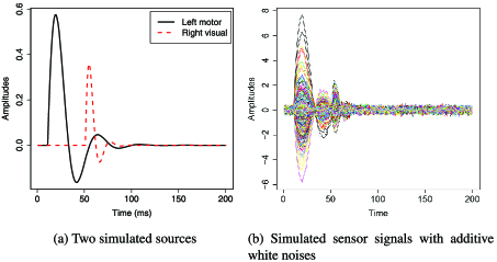
Figure 1: Simulated source and sensor data.

3.2 Comparison criteria

We compare TWR with eight different methods that can be put into two categories as given below.

• One-way regularization:

  • The $L_{2}$-based MNE method [Mosher, Leahy and Lewis (1999)]

  • The $L_{1}$-based MCE method [Matsuura and Okabe (1995)]

  • sOWR (i.e., spatial sparsity only)

  • tOWR (i.e., temporal smoothness only)

• Two-way regularization:

  • The $L_{1}L_{2}$ method proposed by Ou, Hämäläinen and Golland (2009)

  • MNE$+$sOWR (i.e., obtaining the MNE solution as Stage 1 and then applying sOWR)

  • MCE$+$tOWR (i.e., obtaining the MCE solution as Stage 1 and then applying tOWR)

  • MNE$+$TWR (i.e., obtaining the MNE solution as Stage 1 and then applying Stage 2 of TWR)

We put MNE+sOWR in the two-way regularization category because the $L_{2}$ penalty in MNE puts constraints on both domains, and sOWR puts the $L_{1}$ penalty only on the spatial domain. As a result, the temporal domain is regularized by the $L_{2}$ penalty, while the spatial domain is regularized first by the $L_{2}$ penalty and then by the $L_{1}$ penalty. Similarly, MCE+tOWR is also categorized as a two-way regularization method. MNE+sOWR and MCE+tOWR can be considered as two alternative ways for two-way regularization and are suggested by a reviewer. MNE+TWR, also suggested by a reviewer, is a slight modification of TWR, replacing the first stage of TWR by MNE. Its inclusion in comparison helps us study the effect of using a different Stage 1 estimator on the performance of TWR. We implemented all the methods in R, and the tuning parameters are selected using either CV or GCV.

Three comparison criteria are utilized: the overall mean squared error (MSE), the standardized distance between the energy peak of the estimated source and the energy peak of the true source, and the computation time.

The overall MSE is defined as

$$\mathit{MSE}=\frac{1}{p}\|{\mathbf{B}}-\tilde{{\mathbf{B}}}\|^{2}_{F},$$

where ${\mathbf{B}}$ and $\tilde{\mathbf{B}}$ are the true and recovered source matrices, respectively.

Table 1: Comparison of nine methods using four criteria: the mean squared error (MSE), the standardized distance between the true energy peak and the estimated energy peak at the left motor area ($d_{25}$), at the right visual area ($d_{58}$), and the computation time (in seconds). Reported are the average and standard error of each criterion based on 100 simulation runs

Method	MSE ($\bm{10^{-3}}$)	$\bm{d_{25}}$ ($\bm{\times 10^{-4}}$)	$\bm{d_{58}}$ ($\bm{\times 10^{-4}}$)	Computation time (sec.)
MNE	$544.0\ (9.0)$	$50.2\ (7.3)$	$42.9\ (5.9)$	$4371\ (4.3)$
MCE	$903.7\ (8.9)$	$337.1\ (6.4)$	$156.1\ (11.4)$	$1545\ (3.0)$
tOWR	$407.9\ (8.9)$	$40.2\ (5.8)$	$39.6\ (4.3)$	$1841\ (3.4)\tabnoteref$
sOWR	$153.2\ (7.7)$	$19.3\ (4.6)$	$13.9\ (3.9)$	$1798\ (3.6)\tabnoteref{tb1}$
TWR	22.3 (5.7)0	15.7 (3.3)	7.1 (2.4)	$1872\ (3.5)\tabnoteref{tb1}$
$L_{1}L_{2}$	$44.3\ (7.1)$	$31.0\ (6.1)$	$17.8\ (2.3)$	$40\mbox{,}872\ (8.8)$
MNE+sOWR	$187.3\ (8.8)$	$27.9\ (6.8)$	$14.5\ (3.1)$	$5998\ (3.9)$
MCE+tOWR	$912.7\ (10.9)$	$343.8\ (6.2)$	$145.2\ (12.7)$	$3321\ (3.8)$
MNE+TWR	$28.6\ (7.2)$	$16.9\ (4.3)$	$10.7\ (3.9)$	$6201\ (3.1)$

tb1The computation time for each simulation run is computed based on 15 iterations, which are usually more than needed for algorithm convergence.

The energy of the dipole $j$ at time point $k$ is defined as $(b_{jk,x}^{2}+b_{jk,y}^{2}+b_{jk,z}^{2})^{1/2}$, where $b_{jk,x},~{}b_{jk,y},~{}b_{jk,z}~{}(j=1,\ldots,p,~{}k=1,\ldots,s)$, are the amplitude components for the $j$th dipole at the time point $k$ in the Cartesian coordinate system. The energy of the reconstructed source can be defined similarly. The standardized distance between the estimated and the true energy peak at time point $k$ is defined as

$$d_{k}=\frac{\sqrt{(x^{*}_{k}-\hat{x}_{k})^{2}+(y^{*}_{k}-\hat{y}_{k})^{2}+(z^{*}_{k}-\hat{z}_{k})^{2}}}{p/3},$$

where $p/3$ is the total number of dipoles, $x^{*}_{k},~{}y^{*}_{k},~{}z^{*}_{k}$ are the coordinates of the location for the maximum source energy at time point $k$, and $\hat{x},~{}\hat{y},~{}\hat{z}$ are the coordinates for the maximum estimated source energy at the corresponding time point. In this simulation example, there are two peak times, 25 ms and 58 ms, so we are interested in $d_{25}$ and $d_{58}$.

3.3 Results

The simulation was conducted 100 times with the noise term in Model (1) newly generated for each run. The criteria described in the previous subsection (i.e., MSE, $d_{25}$, $d_{58}$, computation time) were evaluated for each simulation run, and the mean and standard error of the criterion values across the 100 runs were calculated. The numerical results are shown in Table 3.2.

Several interesting observations can be made from the table. TWR is the best method in the sense of having the smallest MSE and the shortest distances between the true and the estimated peaks. Among the four one-way regularization methods, sOWR and tOWR outperform the classical MNE and MCE methods, and tOWR outperforms sOWR. The fact that TWR outperforms the four one-way regularization methods justifies our proposal of using two-way regularization. The $L_{1}L_{2}$ method is the third most accurate method, but its computation time is more than 21 times as large as that of TWR. MNE+sOWR and MCE+tOWR are less satisfactory, demonstrating the importance of the first stage. MNE+sOWR is not better than sOWR because the $L_{2}$ penalty of MNE does not smooth the temporal domain. The performance of MCE+tOWR is similar to MCE and is not better than tOWR because MCE does not recover well important information at the first stage, and hence tOWR based on MCE is inaccurate. Note that the reported computation time for TWR, sOWR and tOWR are based on fixed 15 iterations in order to make the calculation of the average computation time meaningful. Such report is conservative because these algorithms usually converge rapidly and fewer iterations (usually less than 10) are enough to obtain considerably good accuracy.

Figures 2 and 3 show the 3-D brain mapping by different methods at 25 ms and 58 ms for a randomly selected simulation run. TWR performs the best among the nine methods in detecting the true source locations even though it misses some small regions. It is able to identify the majority parts of both source locations, and its solutions are focal. Solutions from sOWR and MNE+sOWR are more scattered than TWR. MNE and tOWR produce even more diffuse solutions. MCE misses the main parts of both active areas and so does MCE+tOWR, and they are the least satisfactory methods. The $L_{1}L_{2}$ method recovers some of the activity, but the solution is overly focal. The plot of MNE+TWR is very similar to that of TWR, so it is not presented here to save space. Direct comparison of results of TWR and tOWR clearly demonstrate the positive effect of using regularization in the spatial domain.

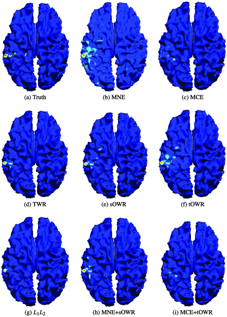
Figure 2: Overviews of brain mapping by different methods at 25 ms. (a) shows the true map, indicating an active area located at the left motor area. TWR identifies the major active area and the solution is focal. The $L_{1}L_{2}$ method also identifies the active area but the solution is too focal. sOWR and MNE+sOWR produce more scattering solutions than TWR. MNE and tOWR detected active areas are diffuse. MCE and MCE+tOWR misidentify the active region.

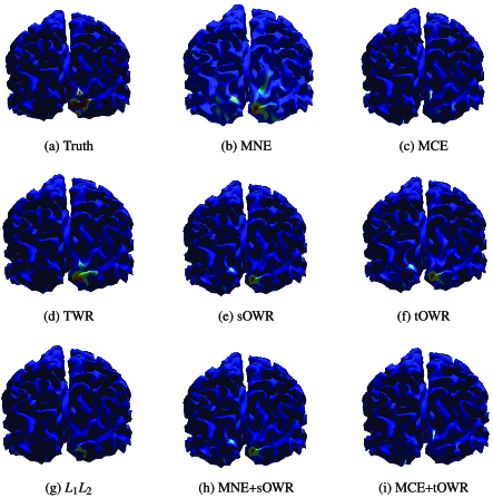
Figure 3: Sideviews of brain mapping by different methods at 58 ms. (a) shows the true map, indicating an active area located at the right visual area. TWR and $L_{1}L_{2}$ identify the major active area and the solution is focal. sOWR and MNE+sOWR produce more scattering solutions than TWR. MNE and tOWR detected active areas are diffuse. MCE and MCE+tOWR misidentify the active region.

Figures 4 and 5 show the true and the recovered time courses by the nine methods for an arbitrarily chosen single dipole component in the two active areas, respectively, for a randomly selected simulation run. Each subfigure shows the true time course and the estimated time course by one method. As one can see, the methods considering the temporal smoothness reconstruct the shape of the source time course well. TWR, tOWR, $L_{1}L_{2}$, MCE+tOWR and MNE+TWR all produce smooth time courses. TWR recovers the most energy of the source, while MCE+tOWR recovers the least. MNE+TWR tends to overshrink the amplitude of the time course because MNE overshrinks the amplitude. The methods without considering the roughness regularization in the temporal domain result in noisy time courses even though some methods can recover the general trend. In Figure 5(b), MCE does not capture the major peaks of the signal, and, consequently, MCE+tOWR [Figure 5(h)], which relies on the solution of MCE, does not recover any signal activity either. Direct comparison of results of TWR and sOWR clearly demonstrate the positive effect of using regularization in the time domain.

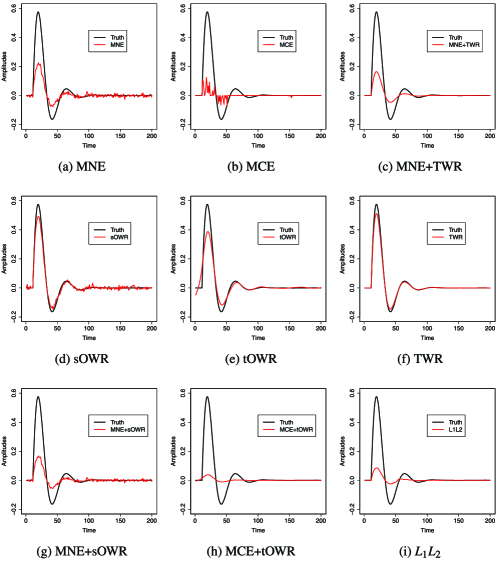
Figure 4: Estimated time courses for one arbitrarily chosen dipole component at left motor area by different methods for a randomly selected simulation run. TWR, tOWR, MCE+tOWR, $L_{1}L_{2}$ and MNE+TWR recover the shape of the time course reasonably well and the solutions are smooth. But MCR+tOWR, MNE+TWR and $L_{1}L_{2}$ overshrink the amplitude. MNE, MCE, sOWR and MNE+sOWR estimate the general trend reasonably well, but the estimated time courses are too noisy. TWR gives the best result.

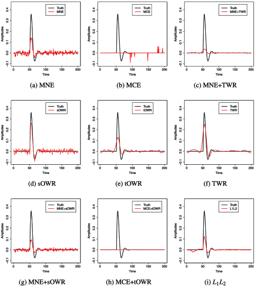
Figure 5: Estimated time courses for one arbitrarily chosen dipole component at right visual area by different methods for a randomly selected simulation run. TWR, tOWR, $L_{1}L_{2}$ and MNE+TWR recover the shape of the time course reasonably well and the solutions are smooth. But MNE+TWR overshrinks the amplitude. MNE, sOWR and MNE+sOWR estimate the general trend reasonably well, but the estimated time courses are too noisy. MCE and MCE+tOWR do not recover the shape of the time course. TWR gives the best result.

The selection of the focality parameter and the roughness penalty parameter was conducted using the method presented in Section 2.4. Figure 6(a) and (b) shows the CV and GCV scores for TWR as functions of $\mu_{1}$ and $\mu_{2}$, respectively. The optimal values of the tuning parameters are $\mu_{1}=0.33$ and $\mu_{2}=5.9$. Figure 6(c) shows the sparsity level of the reconstructed source matrix, $\tilde{{\mathbf{B}}}$, for TWR as a function of the number of iterations when the tuning parameters are set at the selected values. The sparsity level for a matrix is defined as the number of zero entries over the total number of entries. Here the total number of entries for $\tilde{{\mathbf{B}}}$ is $p\times s=3\mbox{,}072\mbox{,}000$. From this figure, we observe that the sparsity of $\tilde{{\mathbf{B}}}$ levels off rather rapidly and stays steadily at about 0.996, a fairly high sparsity level. In fact, this sparsity level matches closely the true level in the simulation setup: The number of true source dipoles is 20, and so the total number of active source components is 60 after considering orientations. Thus, the true sparsity level is $1-60/p=1-60/15360\approx 0.996$.

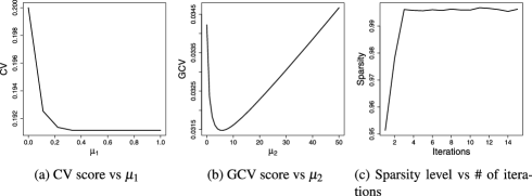
Figure 6: Selection of $\mu_{1}$ and $\mu_{2}$ and the sparsity level as a function of the number of iterations. The optimal $\mu_{1}$ and $\mu_{2}$ are around 0.33 and 5.9, respectively. The sparsity measure levels off at around 0.996.

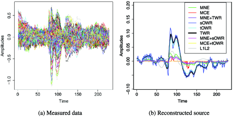
Figure 7: MEG data. (a) MEG recordings from 247 valid channels; (b) Reconstructed time courses from an arbitrary source location in the somatosensory area by different methods.

4 Real data example

In this section we demonstrate the proposed method using a human MEG data set obtained from the Center for Clinical Neurosciences at the University of Texas Health Science Center at Houston. The study subject is a 44-year-old female patient with grade three left frontal astrocytoma who underwent the MEG test as part of the presurgical evaluation. The patient underwent a somatosensory task which is designed to noninvasively identify the somatosensory areas of the patient. We choose this study because of the clinical usefulness of the somatosensory task in presurgical mapping.

Data collection was done with a whole-head neuromagnetometer containing 248 first-order axial gradiometers. During the MEG somatosensory session, 558 repeated stimulations were delivered to the patient’s right lower lip through a pneumatically driven soft plastic diaphragm. Each stimulation lasted 40 ms with 450 ms epoch duration (including a prestimulus baseline of 100 ms) and an interstimulus interval randomized between 0.5 s and 0.6 s. We removed the offset and averaged the 558 epochs to obtain the final event-related magnetic field response. Then a bad channel was removed. The MEG device recorded 228 time points in each epoch. The measurement matrix ${\mathbf{Y}}$ is $247\times 228$, where $n=247$ is the number of valid MEG channels and $s=228$ is the number of recorded data points per epoch. The $n\times p$ forward operator ${\mathbf{X}}$ was obtained using the MNE software with $p=15\mbox{,}372$.

The measured MEG recordings from the 247 valid channels are plotted in Figure 7(a). Among the 228 time points, there are two peaks at time points 85 and 99, corresponding to the activation of the primary somatosensory area contralateral to the stimuli, as expected by clinical experiences and brain anatomic theories.

Nine methods, MNE, MCE, TWR, tOWR, sOWR, MNE+TWR,MNE+sOWR, MCE+tOWR and $L_{1}L_{2}$, were applied to solve the MEG inverse problem. Figure 7(b) shows the reconstructed time courses for an arbitrary source location by different methods. As we can see, TWR, sOWR and tOWR, are satisfactory in terms of estimating the shape of the source time course and capturing the peak features at time points 85 and 99. But sOWR produces a noisy time course. MNE and MNE+sOWR overshrink the magnitudes in addition to producing a noisy time course. MNE+TWR recovers the shape of the time course but underestimates the amplitude. The $L_{1}L_{2}$ method does not distinguish the two peaks. MCE only identifies the first peak but misses the second one. MCE+tOWR does not capture any activity because it smoothes the spikes caused by MCE and hence is the least satisfactory method.

Figure 8 shows the side views of the brain mapping at time point 85 by different methods. As we can see, the somatosensory area was correctly identified by TWR, which matches the clinical expectation. As with the synthetic example, tOWR and MNE produce diffuse solutions, leading to false positives around the somatosensory area. sOWR produces a scattering solution and so does MNE+sOWR. MNE+TWR and $L_{1}L_{2}$ also identify some activity in the frontal lobe. Solutions from MCE and MCE+tOWR are too focal and do not cover the somatosensory area.

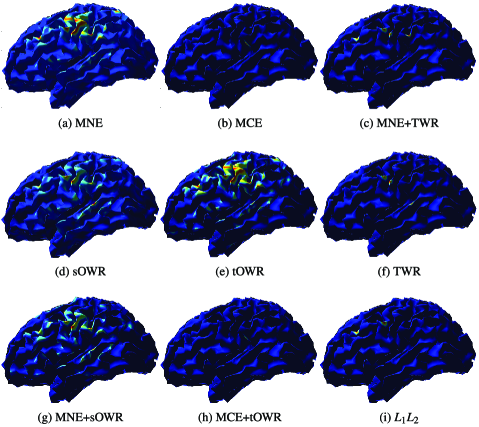
Figure 8: Side views of the brain mapping at time point 85 by different methods. TWR provides a focal and accurate detection; MNE+TWR and $L_{1}L_{2}$ identify some activity in the frontal lobe in addition to the somatosensory area. Solutions from MNE, sOWR, tOWR and MNE+sOWR are too diffuse to be satisfactory. Both MCE and MCE+tOWR miss the activity in the somatosensory area.

Figure 9(a) shows the CV error as a function of $\mu_{1}$. The CV error was minimized when the sparsity parameter, $\mu_{1}$, is about 0.44. Figure 9(b) displays the GCV error as a function of $\mu_{2}$. It shows that the optimal $\mu_{2}$ is about 59.5. The sparsity level as a function of the number of iterations is shown in Figure 9(c). As we can see, the sparsity level increases at first and then levels off rapidly, indicating the algorithm converges fast. The optimal sparsity level was about 0.999.

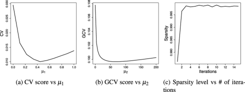
Figure 9: Selection of $\mu_{1}$ and $\mu_{2}$ and the sparsity level as a function of the number of iterations. The optimal $\mu_{1}$ and $\mu_{2}$ are around 0.44 and 59.5, respectively. The sparsity measure levels off at around 0.999.

5 Discussion

TWR solves the MEG inverse problem by using two-way penalties that promote both the temporal smoothness and the spatial focality of the solution. We developed a computational efficient two-stage procedure for implementing TWR. We also considered a one-stage approach that tries to recover the source signal matrix ${\mathbf{B}}={\mathbf{A}}{\mathbf{G}}^{T}$ by solving

$$\min_{{\mathbf{A}},{\mathbf{G}}}\{\|{\mathbf{Y}}-{\mathbf{X}}{\mathbf{A}}{\mathbf{G}}^{T}\|_{F}^{2}+\mu_{1}|{\mathbf{A}}|+\mu_{2}\operatorname{tr}({\mathbf{G}}^{T}\bm{\Omega}{\mathbf{G}})\}.$$ (24)

The optimal matrices ${\mathbf{A}}$ and ${\mathbf{G}}$ can be obtained by alternating optimization. When fixing ${\mathbf{A}}$ as $\hat{{\mathbf{A}}}$, the optimal ${\mathbf{G}}$ can be obtained as in Algorithm 1, as described in Section 2.3. When fixing ${\mathbf{G}}$ as $\hat{{\mathbf{G}}}$, the problem (24)becomes

$$\min_{{\mathbf{A}}}\{\|{\mathbf{Y}}-{\mathbf{X}}{\mathbf{A}}\hat{{\mathbf{G}}}^{T}\|_{F}^{2}+\mu_{1}|{\mathbf{A}}|\}$$

$$\qquad=\min_{{\mathbf{A}}}\{\operatorname{tr}[\hat{\mathbf{G}}({\mathbf{Y}}\hat{\mathbf{G}}-{\mathbf{X}}{\mathbf{A}})^{T}({\mathbf{Y}}\hat{\mathbf{G}}-{\mathbf{X}}{\mathbf{A}})\hat{\mathbf{G}}^{T}]+\mu_{1}|{\mathbf{A}}|\}$$ (25)

$$\qquad=\min_{{\mathbf{A}}}\{\|{\mathbf{Y}}\hat{\mathbf{G}}-{\mathbf{X}}{\mathbf{A}}\|_{F}^{2}+\mu_{1}|{\mathbf{A}}|\},$$

which is equivalent to $s$ different problems, one for each column of ${\mathbf{A}}$, namely,

$$\min_{{\mathbf{a}}_{j}}\{\|{\mathbf{Y}}\hat{\mathbf{g}}_{j}-{\mathbf{X}}{\mathbf{a}}_{j}\|^{2}+\mu_{1}|{\mathbf{a}}_{j}|\},\qquad j=1,\ldots,s,$$

where $\hat{\mathbf{g}}_{j}$ is the $j$th column of the matrix $\hat{{\mathbf{G}}}$. Each of these problems is a standard LASSO regression problem [Tibshirani (1996)] with over 10,000 variables. Although efficient computational algorithms exist for the LASSO regression, the fact that the LASSO problem needs to be solved a few hundred times during each iteration of updating ${\mathbf{A}}$ makes this approach computationally unattractive. Developing a scalable algorithm for the one-stage approach is an important issue for its practical application and remains an interesting research topic.

Acknowledgments

The authors thank the Editor, the Associate Editor and two referees for their comments, which helped improve the scope and presentation of the manuscript. The authors thank the MEG Lab at the University of Texas Health Science Center Houston for providing the data. In particular, thanks are due to Professors Andrew Papanicolaou and Eduardo Castillo for their suggestions and comments.

References

- Auranen et al. (2005) {barticle}[author] \bauthor\bsnmAuranen, \bfnmT.\binitsT., \bauthor\bsnmNummenmaa, \bfnmA.\binitsA., \bauthor\bsnmHämäläinen, \bfnmM. S.\binitsM. S., \bauthor\bsnmJääskeläinen, \bfnmI. P.\binitsI. P., \bauthor\bsnmLampinen, \bfnmJ.\binitsJ., \bauthor\bsnmVehtari, \bfnmA.\binitsA. and \bauthor\bsnmSams, \bfnmM.\binitsM. (\byear2005). \btitleBayesian analysis of the neuromagnetic inverse problem with lp-norm priors. \bjournalNeuroImage \bvolume26 \bpages870–884. \bptokimsref \endbibitem
- Baillet and Garnero (1997) {barticle}[author] \bauthor\bsnmBaillet, \bfnmS.\binitsS. and \bauthor\bsnmGarnero, \bfnmL.\binitsL. (\byear1997). \btitleA Bayesian approach to introducing anatomo-functional prior in the EEG/MEG inverse problem. \bjournalIEEE Transactions on Biomedical Engineering \bvolume44 \bpages374–385. \bptokimsref \endbibitem
- Baillet et al. (2001) {barticle}[pbm] \bauthor\bsnmBaillet, \bfnmS.\binitsS., \bauthor\bsnmRiera, \bfnmJ. J.\binitsJ. J., \bauthor\bsnmMarin, \bfnmG.\binitsG., \bauthor\bsnmMangin, \bfnmJ. F.\binitsJ. F., \bauthor\bsnmAubert, \bfnmJ.\binitsJ. and \bauthor\bsnmGarnero, \bfnmL.\binitsL. (\byear2001). \btitleEvaluation of inverse methods and head models for EEG source localization using a human skull phantom. \bjournalPhys. Med. Biol. \bvolume46 \bpages77–96. \bidissn=0031-9155, pmid=11197680 \bptokimsref \endbibitem
- Barlow (1994) {bincollection}[author] \bauthor\bsnmBarlow, \bfnmHorace B.\binitsH. B. (\byear1994). \btitleWhat is the computational goal of the neocortex? In \bbooktitleLarge-Scale Neuronal Theories of the Brain (\beditor\bfnmC.\binitsC. \bsnmKoch and \beditor\bfnmJ. L.\binitsJ. L. \bsnmDavis, eds.) \bpages1–22. \bpublisherMIT press, \baddressCambridge, MA. \bptokimsref \endbibitem
- Bolstad, Veen and Nowak (2009) {barticle}[author] \bauthor\bsnmBolstad, \bfnmAndrew\binitsA., \bauthor\bsnmVeen, \bfnmBarry Van\binitsB. V. and \bauthor\bsnmNowak, \bfnmRobert\binitsR. (\byear2009). \btitleSpace-time event sparse penalization for magneto-/electroencephalography. \bjournalNeuroImage \bvolume46 \bpages1066–1081. \bptokimsref \endbibitem
- Brent (1973) {bbook}[mr] \bauthor\bsnmBrent, \bfnmRichard P.\binitsR. P. (\byear1973). \btitleAlgorithms for Minimization Without Derivatives. \bpublisherPrentice-Hall Inc., \baddressEnglewood Cliffs, NJ. \bidmr=0339493 \bptokimsref \endbibitem
- Darvas et al. (2004) {barticle}[author] \bauthor\bsnmDarvas, \bfnmF.\binitsF., \bauthor\bsnmPantazis, \bfnmD.\binitsD., \bauthor\bsnmKucukaltun-Yildirim, \bfnmE.\binitsE. and \bauthor\bsnmLeahy, \bfnmR. M.\binitsR. M. (\byear2004). \btitleMapping human brain function with MEG and EEG: Methods and validation. \bjournalNeoroImage \bvolume23 \bpages289–299. \bptokimsref \endbibitem
- Daunizeau et al. (2006) {barticle}[pbm] \bauthor\bsnmDaunizeau, \bfnmJean\binitsJ., \bauthor\bsnmMattout, \bfnmJérémie\binitsJ., \bauthor\bsnmClonda, \bfnmDiego\binitsD., \bauthor\bsnmGoulard, \bfnmBernard\binitsB., \bauthor\bsnmBenali, \bfnmHabib\binitsH. and \bauthor\bsnmLina, \bfnmJean-Marc\binitsJ.-M. (\byear2006). \btitleBayesian spatio-temporal approach for EEG source reconstruction: Conciliating ECD and distributed models. \bjournalIEEE Trans. Biomed. Eng. \bvolume53 \bpages503–516. \biddoi=10.1109/TBME.2005.869791, issn=0018-9294, pmid=16532777 \bptokimsref \endbibitem
- Ding and He (2008) {barticle}[pbm] \bauthor\bsnmDing, \bfnmLei\binitsL. and \bauthor\bsnmHe, \bfnmBin\binitsB. (\byear2008). \btitleSparse source imaging in electroencephalography with accurate field modeling. \bjournalHum. Brain Mapp \bvolume29 \bpages1053–1067. \biddoi=10.1002/hbm.20448, issn=1097-0193, mid=NIHMS59224, pmcid=2612127, pmid=17894400 \bptokimsref \endbibitem
- Dogandžić and Nehorai (2000) {barticle}[author] \bauthor\bsnmDogandžić, \bfnmAleksandar\binitsA. and \bauthor\bsnmNehorai, \bfnmArye\binitsA. (\byear2000). \btitleEstimating evoked dipole responses in unknown spatially correlated noise with EEG/MEG arrays. \bjournalIEEE Trans. Signal Process. \bvolume48 \bpages13–25. \bptokimsref \endbibitem
- Friston et al. (2008) {barticle}[author] \bauthor\bsnmFriston, \bfnmK\binitsK., \bauthor\bsnmHarrison, \bfnmL\binitsL., \bauthor\bsnmDaunizeau, \bfnmJ\binitsJ., \bauthor\bsnmKiebel, \bfnmS\binitsS., \bauthor\bsnmPhillips, \bfnmC\binitsC., \bauthor\bsnmTrujillo-Barreto, \bfnmN\binitsN., \bauthor\bsnmHenson, \bfnmR\binitsR., \bauthor\bsnmFlandin, \bfnmG\binitsG. and \bauthor\bsnmMattout, \bfnmJ.\binitsJ. (\byear2008). \btitleMultiple sparse priors for the M/EEG inverse problem. \bjournalNeuroImage \bvolume39 \bpages1104–1120. \bptokimsref \endbibitem
- Gorodnitsky and Rao (1997) {barticle}[author] \bauthor\bsnmGorodnitsky, \bfnmI. F.\binitsI. F. and \bauthor\bsnmRao, \bfnmB. D.\binitsB. D. (\byear1997). \btitleSparse signal reconstruction from limited data using FOCUSS: A re-weighted minimum norm algorithm. \bjournalIEEE Transactions on Signal Processing \bvolume45 \bpages600–616. \bptokimsref \endbibitem
- Hämäläinen and Ilmoniemi (1994) {btechreport}[author] \bauthor\bsnmHämäläinen, \bfnmMatti\binitsM. and \bauthor\bsnmIlmoniemi, \bfnmRisto J.\binitsR. J. (\byear1994). \btitleInterpreting measured magnetic fields of the brain: Estimates of current distribution. \btypeTechnical Report TKK-F-A599, \binstitutionHelsinki Univ. Technology. \bptokimsref \endbibitem
- Hämäläinen et al. (1993) {barticle}[author] \bauthor\bsnmHämäläinen, \bfnmMatti\binitsM., \bauthor\bsnmHari, \bfnmRiitta\binitsR., \bauthor\bsnmIlmoniemi, \bfnmRisto J.\binitsR. J., \bauthor\bsnmKnuutila, \bfnmJukka\binitsJ. and \bauthor\bsnmLounasmaa, \bfnmOlli V.\binitsO. V. (\byear1993). \btitleMagnetoencephalography-theory, instrumentation, and applications to noninvasive studies of the working human brain. \bjournalRev. Modern Phys. \bvolume65 \bpages413–497. \bptokimsref \endbibitem
- Huang, Shen and Buja (2008) {barticle}[mr] \bauthor\bsnmHuang, \bfnmJianhua Z.\binitsJ. Z., \bauthor\bsnmShen, \bfnmHaipeng\binitsH. and \bauthor\bsnmBuja, \bfnmAndreas\binitsA. (\byear2008). \btitleFunctional principal components analysis via penalized rank one approximation. \bjournalElectron. J. Stat. \bvolume2 \bpages678–695. \biddoi=10.1214/08-EJS218, issn=1935-7524, mr=2426107 \bptokimsref \endbibitem
- Huang, Shen and Buja (2009) {barticle}[mr] \bauthor\bsnmHuang, \bfnmJianhua Z.\binitsJ. Z., \bauthor\bsnmShen, \bfnmHaipeng\binitsH. and \bauthor\bsnmBuja, \bfnmAndreas\binitsA. (\byear2009). \btitleThe analysis of two-way functional data using two-way regularized singular value decompositions. \bjournalJ. Amer. Statist. Assoc. \bvolume104 \bpages1609–1620. \biddoi=10.1198/jasa.2009.tm08024, issn=0162-1459, mr=2750581 \bptokimsref \endbibitem
- Jeffs, Leahy and Singh (1987) {barticle}[pbm] \bauthor\bsnmJeffs, \bfnmB.\binitsB., \bauthor\bsnmLeahy, \bfnmR.\binitsR. and \bauthor\bsnmSingh, \bfnmM.\binitsM. (\byear1987). \btitleAn evaluation of methods for neuromagnetic image reconstruction. \bjournalIEEE Trans. Biomed. Eng. \bvolume34 \bpages713–723. \bidissn=0018-9294, pmid=3653912 \bptokimsref \endbibitem
- Jun et al. (2005) {barticle}[author] \bauthor\bsnmJun, \bfnmSung C\binitsS. C., \bauthor\bsnmGeorge, \bfnmJohn S\binitsJ. S., \bauthor\bsnmPaŕe-Blagoev, \bfnmJuliana\binitsJ., \bauthor\bsnmPlis, \bfnmSergey M\binitsS. M., \bauthor\bsnmRanken, \bfnmDoug M\binitsD. M., \bauthor\bsnmSchmidt, \bfnmDavid M\binitsD. M. and \bauthor\bsnmWood, \bfnmC C\binitsC. C. (\byear2005). \btitleSpatiotemporal Bayesian inference dipole analysis for MEG neuroimaging data. \bjournalNeuroImage \bvolume29 \bpages84–98. \bptokimsref \endbibitem
- Lee et al. (2010) {barticle}[mr] \bauthor\bsnmLee, \bfnmMihee\binitsM., \bauthor\bsnmShen, \bfnmHaipeng\binitsH., \bauthor\bsnmHuang, \bfnmJianhua Z.\binitsJ. Z. and \bauthor\bsnmMarron, \bfnmJ. S.\binitsJ. S. (\byear2010). \btitleBiclustering via sparse singular value decomposition. \bjournalBiometrics \bvolume66 \bpages1087–1095. \biddoi=10.1111/j.1541-0420.2010.01392.x, issn=0006-341X, mr=2758496 \bptokimsref \endbibitem
- Lin et al. (2006) {barticle}[pbm] \bauthor\bsnmLin, \bfnmFa-Hsuan\binitsF.-H., \bauthor\bsnmBelliveau, \bfnmJohn W.\binitsJ. W., \bauthor\bsnmDale, \bfnmAnders M.\binitsA. M. and \bauthor\bsnmHämäläinen, \bfnmMatti S.\binitsM. S. (\byear2006). \btitleDistributed current estimates using cortical orientation constraints. \bjournalHum. Brain Mapp \bvolume27 \bpages1–13. \biddoi=10.1002/hbm.20155, issn=1065-9471, pmid=16082624 \bptokimsref \endbibitem
- Lu and Kaufman (2003) {bbook}[author] \bauthor\bsnmLu, \bfnmZ\binitsZ. and \bauthor\bsnmKaufman, \bfnmL\binitsL. (\byear2003). \btitleMagnetic Source Imaging of the Human Brain. \bpublisherawrence Erlbaum Associates, Inc., \baddressManwah, New Jersey. \bptokimsref \endbibitem
- Matsuura and Okabe (1995) {barticle}[pbm] \bauthor\bsnmMatsuura, \bfnmK.\binitsK. and \bauthor\bsnmOkabe, \bfnmY.\binitsY. (\byear1995). \btitleSelective minimum-norm solution of the biomagnetic inverse problem. \bjournalIEEE Trans. Biomed. Eng. \bvolume42 \bpages608–615. \biddoi=10.1109/10.387200, issn=0018-9294, pmid=7790017 \bptokimsref \endbibitem
- Mosher, Leahy and Lewis (1999) {barticle}[pbm] \bauthor\bsnmMosher, \bfnmJ. C.\binitsJ. C., \bauthor\bsnmLeahy, \bfnmR. M.\binitsR. M. and \bauthor\bsnmLewis, \bfnmP. S.\binitsP. S. (\byear1999). \btitleEEG and MEG: Forward solutions for inverse methods. \bjournalIEEE Trans. Biomed. Eng. \bvolume46 \bpages245–259. \bidissn=0018-9294, pmid=10097460 \bptokimsref \endbibitem
- Mosher, Lewis and Leahy (1992) {barticle}[pbm] \bauthor\bsnmMosher, \bfnmJ. C.\binitsJ. C., \bauthor\bsnmLewis, \bfnmP. S.\binitsP. S. and \bauthor\bsnmLeahy, \bfnmR. M.\binitsR. M. (\byear1992). \btitleMultiple dipole modeling and localization from spatio-temporal MEG data. \bjournalIEEE Trans. Biomed. Eng. \bvolume39 \bpages541–557. \biddoi=10.1109/10.141192, issn=0018-9294, pmid=1601435 \bptokimsref \endbibitem
- Nummenmaa et al. (2007a) {barticle}[pbm] \bauthor\bsnmNummenmaa, \bfnmAapo\binitsA., \bauthor\bsnmAuranen, \bfnmToni\binitsT., \bauthor\bsnmHämäläinen, \bfnmMatti S.\binitsM. S., \bauthor\bsnmJääskeläinen, \bfnmIiro P.\binitsI. P., \bauthor\bsnmLampinen, \bfnmJouko\binitsJ., \bauthor\bsnmSams, \bfnmMikko\binitsM. and \bauthor\bsnmVehtari, \bfnmAki\binitsA. (\byear2007a). \btitleHierarchical Bayesian estimates of distributed MEG sources: Theoretical aspects and comparison of variational and MCMC methods. \bjournalNeuroimage \bvolume35 \bpages669–685. \biddoi=10.1016/j.neuroimage.2006.05.001, issn=1053-8119, pii=S1053-8119(06)00537-4, pmid=17300961 \bptokimsref \endbibitem
- Nummenmaa et al. (2007b) {btechreport}[author] \bauthor\bsnmNummenmaa, \bfnmA.\binitsA., \bauthor\bsnmAuranen, \bfnmT.\binitsT., \bauthor\bsnmVanni, \bfnmS.\binitsS., \bauthor\bsnmHämäläinen, \bfnmM. S.\binitsM. S., \bauthor\bsnmJääskeläinen, \bfnmI. P.\binitsI. P., \bauthor\bsnmLampinen, \bfnmJ.\binitsJ., \bauthor\bsnmVehtari, \bfnmA.\binitsA. and \bauthor\bsnmSams, \bfnmM.\binitsM. (\byear2007b). \btitleSparse MEG inverse solutions via hierarchical Bayesian modeling: Evaluation with a parallel fMRI study \btypeTechnical Report B65, \binstitutionLaboratory of Computational Engineering, Helsinki Univ. Technology, \baddressHelsinki, Finland. \bptokimsref \endbibitem
- Nunez (1981) {bbook}[author] \bauthor\bsnmNunez, \bfnmP. L.\binitsP. L. (\byear1981). \btitleElectric Fields of the Brain: The Neurophysics of EEG. \bpublisherOxford Univ. Press, \baddressNew York, NY. \bptokimsref \endbibitem
- Ou, Hämäläinen and Golland (2009) {barticle}[pbm] \bauthor\bsnmOu, \bfnmWanmei\binitsW., \bauthor\bsnmHämäläinen, \bfnmMatti S.\binitsM. S. and \bauthor\bsnmGolland, \bfnmPolina\binitsP. (\byear2009). \btitleA distributed spatio-temporal EEG/MEG inverse solver. \bjournalNeuroimage \bvolume44 \bpages932–946. \biddoi=10.1016/j.neuroimage.2008.05.063, issn=1095-9572, mid=NIHMS90513, pii=S1053-8119(08)00715-5, pmcid=2730457, pmid=18603008 \bptokimsref \endbibitem
- Papanicolaou (1995) {barticle}[pbm] \bauthor\bsnmPapanicolaou, \bfnmA. C.\binitsA. C. (\byear1995). \btitleAn introduction to magnetoencephalography with some applications. \bjournalBrain Cogn. \bvolume27 \bpages331–352. \biddoi=10.1006/brcg.1995.1026, issn=0278-2626, pii=S0278-2626(85)71026-3, pmid=7626280 \bptokimsref \endbibitem
- Pascual-Marqui (2002) {barticle}[author] \bauthor\bsnmPascual-Marqui, \bfnmRoberto Domingo\binitsR. D. (\byear2002). \btitleStandardized low-resolution brain electromagnetic tomography (sLORETA): Technical details. \bjournalMethods & Findings in Experimental & Clinical Pharmacology \bvolume24 \bpages5–12. \bptokimsref \endbibitem
- Pascual-Marqui, Michel and Lehmann (1994) {barticle}[pbm] \bauthor\bsnmPascual-Marqui, \bfnmR. D.\binitsR. D., \bauthor\bsnmMichel, \bfnmC. M.\binitsC. M. and \bauthor\bsnmLehmann, \bfnmD.\binitsD. (\byear1994). \btitleLow resolution electromagnetic tomography: A new method for localizing electrical activity in the brain. \bjournalInt. J. Psychophysiol. \bvolume18 \bpages49–65. \bidissn=0167-8760, pii=0167-8760(84)90014-X, pmid=7876038 \bptokimsref \endbibitem
- Sarvas (1987) {barticle}[pbm] \bauthor\bsnmSarvas, \bfnmJ.\binitsJ. (\byear1987). \btitleBasic mathematical and electromagnetic concepts of the biomagnetic inverse problem. \bjournalPhys. Med. Biol. \bvolume32 \bpages11–22. \bidissn=0031-9155, pmid=3823129 \bptokimsref \endbibitem
- Scherg and Von Cramon (1986) {barticle}[pbm] \bauthor\bsnmScherg, \bfnmM.\binitsM. and \bauthor\bsnmVon Cramon, \bfnmD.\binitsD. (\byear1986). \btitleEvoked dipole source potentials of the human auditory cortex. \bjournalElectroencephalogr. Clin. Neurophysiol. \bvolume65 \bpages344–360. \bidissn=0013-4694, pmid=2427326 \bptokimsref \endbibitem
- Schmidt (1986) {barticle}[author] \bauthor\bsnmSchmidt, \bfnmR. O.\binitsR. O. (\byear1986). \btitleMultiple emitter location and signal parameter estimation. \bjournalIEEE Trans. Antennas and Propagation \bvolume43 \bpages276–280. \bptokimsref \endbibitem
- Shen and Huang (2008) {barticle}[mr] \bauthor\bsnmShen, \bfnmHaipeng\binitsH. and \bauthor\bsnmHuang, \bfnmJianhua Z.\binitsJ. Z. (\byear2008). \btitleSparse principal component analysis via regularized low rank matrix approximation. \bjournalJ. Multivariate Anal. \bvolume99 \bpages1015–1034. \biddoi=10.1016/j.jmva.2007.06.007, issn=0047-259X, mr=2419336 \bptokimsref \endbibitem
- Sorrentino et al. (2009) {barticle}[pbm] \bauthor\bsnmSorrentino, \bfnmAlberto\binitsA., \bauthor\bsnmParkkonen, \bfnmLauri\binitsL., \bauthor\bsnmPascarella, \bfnmAnnalisa\binitsA., \bauthor\bsnmCampi, \bfnmCristina\binitsC. and \bauthor\bsnmPiana, \bfnmMichele\binitsM. (\byear2009). \btitleDynamical MEG source modeling with multi-target Bayesian filtering. \bjournalHum. Brain Mapp \bvolume30 \bpages1911–1921. \biddoi=10.1002/hbm.20786, issn=1097-0193, pmid=19378276 \bptokimsref \endbibitem
- Tibshirani (1996) {barticle}[mr] \bauthor\bsnmTibshirani, \bfnmRobert\binitsR. (\byear1996). \btitleRegression shrinkage and selection via the lasso. \bjournalJ. Roy. Statist. Soc. Ser. B \bvolume58 \bpages267–288. \bidissn=0035-9246, mr=1379242 \bptokimsref \endbibitem
- Uutela, Hämäläinen and Somersalo (1999) {barticle}[pbm] \bauthor\bsnmUutela, \bfnmK.\binitsK., \bauthor\bsnmHämäläinen, \bfnmM.\binitsM. and \bauthor\bsnmSomersalo, \bfnmE.\binitsE. (\byear1999). \btitleVisualization of magnetoencephalographic data using minimum current estimates. \bjournalNeuroimage \bvolume10 \bpages173–180. \biddoi=10.1006/nimg.1999.0454, issn=1053-8119, pii=S1053-8119(99)90454-8, pmid=10417249 \bptokimsref \endbibitem
- VanVeen et al. (1997) {barticle}[author] \bauthor\bsnmVanVeen, \bfnmB.\binitsB., \bauthor\bparticlevan \bsnmDrongelen, \bfnmW.\binitsW., \bauthor\bsnmYuchtman, \bfnmM.\binitsM. and \bauthor\bsnmSuzuki, \bfnmA.\binitsA. (\byear1997). \btitleLocalization of brain electrical activity via linearly constrained minimum variance spatial filtering. \bjournalIEEE Transactions on Biomedical Engineering \bvolume44 \bpages867–880. \bptokimsref \endbibitem
- Veen and Buckley (1988) {barticle}[author] \bauthor\bsnmVeen, \bfnmB. D. V.\binitsB. D. V. and \bauthor\bsnmBuckley, \bfnmK. M.\binitsK. M. (\byear1988). \btitleBeamforming: A versatile approach to spatial filtering. \bjournalIEEE ASSP Magazine \bvolume5 \bpages4–24. \bptokimsref \endbibitem
- von Helmholtz (1853) {barticle}[author] \bauthor\bparticlevon \bsnmHelmholtz, \bfnmH.\binitsH. (\byear1853). \btitleUeber einige Gesetze der Vertheilung elektrischer Ströme in körperlichen Leitern mit Anwendung auf die thierisch-elektrischen Versuche. \bjournalAnn. Phys. \bvolume165 \bpages211–233. \bptokimsref \endbibitem
- Witten, Tibshirani and Hastie (2009) {barticle}[pbm] \bauthor\bsnmWitten, \bfnmDaniela M.\binitsD. M., \bauthor\bsnmTibshirani, \bfnmRobert\binitsR. and \bauthor\bsnmHastie, \bfnmTrevor\binitsT. (\byear2009). \btitleA penalized matrix decomposition, with applications to sparse principal components and canonical correlation analysis. \bjournalBiostatistics \bvolume10 \bpages515–534. \biddoi=10.1093/biostatistics/kxp008, issn=1468-4357, pii=kxp008, pmcid=2697346, pmid=19377034 \bptokimsref \endbibitem
- Yamazaki et al. (2000) {barticle}[pbm] \bauthor\bsnmYamazaki, \bfnmT.\binitsT., \bauthor\bsnmKamijo, \bfnmK.\binitsK., \bauthor\bsnmKenmochi, \bfnmA.\binitsA., \bauthor\bsnmFukuzumi, \bfnmS.\binitsS., \bauthor\bsnmKiyuna, \bfnmT.\binitsT., \bauthor\bsnmTakaki, \bfnmY.\binitsY. and \bauthor\bsnmKuroiwa, \bfnmY.\binitsY. (\byear2000). \btitleMultiple equivalent current dipole source localization of visual event-related potentials during oddball paradigm with motor response. \bjournalBrain Topogr. \bvolume12 \bpages159–175. \bidissn=0896-0267, pmid=10791680 \bptokimsref \endbibitem