UB-ECM-FP-79/12

ICCUB-12-324

Feshbach resonance: a one dimensional example.
Josep Taron
Departament d’Estructura i Constituents de la Matèria
Facultat de Física, Universitat de Barcelona
and
Institut de Ciències del Cosmos
Diagonal 645, E-08028 Barcelona, Spain.

We present a simple one-dimensional example of a spin 1/2 particle submitted to a delta-type potential which interacts differently with the two components of the wavefunction and to an external magnetic field. It has two coupled channels, admits a closed solution and features the Feshbach resonance phehomenon by proper tunning of the magnetic field.

1 Introduction

Consider a spin 1/2 uncharged particle with its motion confined to the $z$-axis only, driven by the hamiltoninan:

$$H=-{\rm{\bf I}}\;\frac{\hbar^{2}}{2m}\frac{d^{2}}{dz^{2}}+\left(\begin{array}[]{cc}V_{1}(z)&0\\ 0&V_{2}(z)\end{array}\right)-\mu B\sigma_{x}.$$

It consists of a kinetic term, a potential term that we assume is short range which interacts differently with the spin up and the spin down components of the wavefuntion and the interaction with a constant external magnetic field that points in the $x$-direction $\vec{B}=(B,0,0)$; $\mu$ is the particle dipole magnetic moment, $\sigma_{x}$ is the $x$ Pauli matrix and $I$ is the $2\times 2$ identity matrix.

The time independent Schödinger equation for such a system reads, in terms of the spin up $\psi(z)$ and the spin down $\varphi(z)$ components of the wavefunction,

$$-\frac{\hbar^{2}}{2m}\frac{d^{2}\psi(z)}{dz^{2}}+V_{1}(z)\;\psi(z)-\mu B\;\varphi(z)=E\;\psi(z),$$

$$-\frac{\hbar^{2}}{2m}\frac{d^{2}\varphi(z)}{dz^{2}}+V_{2}(z)\;\varphi(z)-\mu B\;\psi(z)=E\;\varphi(z),$$ (1)

where $E$ is the total energy of the system. By adding and subtracting these equations one finds,

$$-\frac{\hbar^{2}}{2m}\frac{d^{2}u(z)}{dz^{2}}+V\;u(z)+W\;v(z)=(E+\mu B)\;u(z),$$

$$-\frac{\hbar^{2}}{2m}\frac{d^{2}v(z)}{dz^{2}}+V\;v(z)+W\;u(z)=(E-\mu B)\;v(z),$$ (2)

with,

$$V\equiv\frac{V_{1}+V_{2}}{2},\;\;\;W\equiv\frac{V_{1}-V_{2}}{2},$$ (3)

where the $u=(\psi+\varphi)/\sqrt{2}$ and $v=(\psi-\varphi)/\sqrt{2}$ combinations are the components in the basis of eigenvectors of $\sigma_{x}$, which diagonalize the magnetic part of the interaction and define the spin Zeeman states of the particle, with magnetic energies $\pm\mu B$.

The different channels are defined by specifying these Zeeman states. A channel is said to be open or closed depending on the sign of the combination $E\pm\mu B$ in the r.h.s of (2), positive or negative, respectively. As we shall see, it is crucial that the magnetic energy of the two Zeeman components have opposite signs. This asymetry allows the possibility of having simultaneously one open and one closed channel.

We can think of the coupling interaction term $W$ as a perturbation that modifies the two bare decoupled equations, one for each of the components. It is said that the bare equations are dressed by the coupling $W$.

In a scattering experiment, with an incident beam of pure $u$ component in a remote zone far from the region where the potential acts, the $u$ channel is open and its incident kinetic energy $Q$ corresponds to the combination $Q=E+\mu B$, which can be fixed experimentaly. This in turn fixes the r.h.s. of the second equation too, $E-\mu B=Q-2\mu B$, whose sign can be changed by conveniently tunning the magnitude of the external field $B$.

Finally, notice that the eqs. (2) do not decouple unless $V_{1}=V_{2}$.

2 Delta-type potentials.

We consider attractive delta-type potentials $V_{1}(z)=-g_{1}\delta(z)$ and $V_{2}(z)=-g_{2}\delta(z)$, with $g_{1}\neq g_{2}$, where both $g_{1}$ and $g_{2}$ are taken positive. One can think of it as a mathematical effective substitute that describes the low energy scattering off a pottential which only acts in a small region, much smaller than the wavelength of the scattered particle [5].

In terms of the combinations,

$$\alpha_{1}=\frac{mg_{1}}{\hbar^{2}},\;\;\;\alpha_{2}=\frac{mg_{2}}{\hbar^{2}},\;\;{\rm and}\;\;K^{2}=\frac{2m(E+\mu B)}{\hbar^{2}},\;\;\;\;K^{\prime 2}=\frac{2m(E-\mu B)}{\hbar^{2}},$$ (4)

equations in (2) can be written as,

$$\left(\frac{d^{2}}{dz^{2}}+K^{2}\right)\;u(z)=-S\;\delta(z),\;\;\;\left(\frac{d^{2}}{dz^{2}}+K^{\prime 2}\right)\;v(z)=-S^{\prime}\;\delta(z),$$ (5)

where,

$$S=(\alpha_{1}+\alpha_{2})\;u(0)+(\alpha_{1}-\alpha_{2})\;v(0),\;\;\;\;S^{\prime}=(\alpha_{1}+\alpha_{2})\;v(0)+(\alpha_{1}-\alpha_{2})\;u(0);$$ (6)

beeing $u(0)$, $v(0)$ the values of the wavefunction components at $z=0$, the only place where the potential acts.

There are various possibilities that combine different signs of $K^{2}$ and $K^{\prime 2}$. Of special interest to us is the case with one open channel, coupled to the other channel closed; the first has $K^{2}>0$, whereas the second has $K^{\prime 2}<0$. We set $K^{\prime}=i\beta^{\prime}$, with $\beta^{\prime}$ real and positive. The scattering solution, with the usual incoming wave $\displaystyle e^{iKz}$ at the open channel entrance plus outgoing scattered waves, may be written as (see Appendix),

$$u(z)=e^{iKz}-S\;\frac{e^{iK|z|}}{2iK}=e^{iKz}-\frac{1}{iK}\left[\frac{\alpha_{1}+\alpha_{2}}{2}\;u(0)+\frac{\alpha_{1}-\alpha_{2}}{2}\;v(0)\right]\;e^{iK|z|},$$ (7)

and for the closed channel,

$$v(z)=S^{\prime}\frac{e^{-\beta^{\prime}|z|}}{2\beta^{\prime}}=\frac{1}{\beta^{\prime}}\left[\frac{\alpha_{1}+\alpha_{2}}{2}\;v(0)+\frac{\alpha_{1}-\alpha_{2}}{2}\;u(0)\right]\;e^{-\beta^{\prime}|z|}.$$ (8)

The sources in the r.h.s. of (8) are proportional to the values that the wavefunction components $u(0)$, $v(0)$ take at the origin, which can be obtained self-consistently from (8) by setting $z=0$ and solving the resulting linear system. We obtain,

$$v(0)=\frac{1}{2}\;\frac{\alpha_{1}-\alpha_{2}}{\displaystyle\beta^{\prime}-\frac{\alpha_{1}+\alpha_{2}}{2}}\;u(0),$$ (9)

and from the first equation in (8),

$$u(z)=e^{iKz}-\alpha_{\rm{eff}}(\beta^{\prime})u(0)\;\frac{e^{iK|z|}}{iK}.$$ (10)

where we have defined,

$$\alpha_{\rm{eff}}(\beta^{\prime})=\frac{\alpha_{1}+\alpha_{2}}{2}+\frac{1}{4}\;\frac{\displaystyle\left(\alpha_{1}-\alpha_{2}\right)^{2}}{\displaystyle\beta^{\prime}-\frac{\alpha_{1}+\alpha_{2}}{2}}.$$ (11)

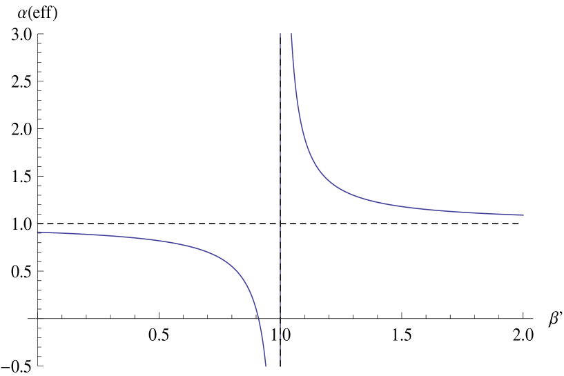
Figure 1: Plot of $\displaystyle\alpha_{{\rm eff}}(\beta^{\prime})$ in (11). For fixed $K$, by varying the magnetic field $B$ and thus $0\leq\beta^{\prime}<\infty$, $\displaystyle\alpha_{{\rm eff}}$ can take on any value in the full range, $-\infty<\alpha_{{\rm eff}}<+\infty$. Notice the pole at $\beta_{{\rm pole}}^{\prime}$, and the value of $\beta_{c}^{\prime}$ at which $\displaystyle\alpha_{{\rm eff}}$ vanishes. [The plot corresponds to the values $\alpha_{1}=1.3$, $\alpha_{2}=0.7$ in units of inverse length $\displaystyle\left[(\alpha_{1}+\alpha_{2})/2\right]$ - which corresponds to the inverse of the spatial extension of the wavefunction closed channel component (21) at the Feshbach resonance. We have $\beta^{\prime}_{c}=0.91$ and $\beta_{{\rm pole}}=1$ in such units. ]

Equations (10) and (11) summarize the remarkable result that we wish to emphasize: the net result of the two coupled channels, with one channel open and the other one closed, is equivalent to a single channel one-dimensional scattering problem with wavenumber $K$ and an effective delta-type potential given by (see Appendix),

$$V_{{\rm eff}}(z)=-g_{{\rm eff}}(\beta^{\prime})\;\delta(z),\;\;{\rm with\;\;coupling}\;\;g_{\rm{eff}}(\beta^{\prime})\equiv\frac{\hbar^{2}}{m}\alpha_{\rm{eff}}(\beta^{\prime}),$$ (12)

that depends on $\displaystyle\beta^{\prime}(K,B)=\sqrt{\frac{2m}{\hbar^{2}}(2\mu B)-K^{2}}$. Therefore, for fixed $K$ any value in the whole range, $-\infty<\alpha_{\rm{eff}}(\beta^{\prime})<+\infty$, is available for the effective coupling by varying $B$ (see Fig. 1). This effect disappears completely if $\alpha_{1}=\alpha_{2}$, in which case the equations in (2) are not coupled anymore.

We find,

$$u(0)=\frac{1}{1+{\displaystyle\frac{\alpha_{{\rm eff}}(\beta^{\prime})}{iK}}},$$ (13)

and the complete solution (8) reads,

$$u(z)=e^{iKz}+r(K,\beta^{\prime})e^{iK|z|},\;\;\;{\rm with}\;\;r(K,\beta^{\prime})=-\frac{\alpha_{{\rm eff}}(\beta^{\prime})}{iK+\alpha_{{\rm eff}}(\beta^{\prime})},$$ (14)

where $r(K,\beta^{\prime})$ and $t(K,\beta^{\prime})=1+r(K,\beta^{\prime})$ are the reflection and the transmission amplitudes, respectively. For the other component,

$$v(z)=v(0)e^{-\beta^{\prime}|z|}=\frac{iK\left(\displaystyle{\frac{\alpha_{1}-\alpha_{2}}{2}}\right)}{\left(iK+\displaystyle{\frac{\alpha_{1}+\alpha_{2}}{2}}\right)\left(\beta^{\prime}-\displaystyle{\frac{\alpha_{1}+\alpha_{2}}{2}}\right)+\left({\displaystyle{\frac{\alpha_{1}-\alpha_{2}}{2}}}\right)^{2}}\;e^{-\beta^{\prime}|z|}.$$ (15)

There is a value $\beta^{\prime}_{c}$ which makes the effective coupling vanish, $\alpha_{\rm{eff}}(\beta_{c}^{\prime})=0$,

$$\frac{1}{\beta_{c}^{\prime}}=\frac{1}{2}\left(\frac{1}{\alpha_{1}}+\frac{1}{\alpha_{2}}\right),$$ (16)

where the net effective interaction in the open channel disappears and $r(K,\beta^{\prime}_{c})=0$. The wave function becomes,

$$u(z)=e^{iKz},\;\;v(z)=-\frac{\alpha_{1}+\alpha_{2}}{\alpha_{1}-\alpha_{2}}\;e^{-\beta^{\prime}_{c}|z|},$$ (17)

with a persisting presence in the closed channel in spite of $\alpha_{{\rm eff}}(\beta^{\prime}_{c})$ being zero.

Moreover, $\alpha_{\rm{eff}}(\beta^{\prime})$ has a pole at,

$$\beta_{{\rm pole}}^{\prime}=\frac{(\alpha_{1}+\alpha_{2})}{2},$$ (18)

where it diverges, which leads to total reflection for any value of $K$, $r(K,\beta^{\prime}_{{\rm pole}})=1$, with no transmission whatsoever. This is the Feshbach resonant solution. Its wavefunction is,

$$u(z)=e^{iKz}-e^{iK|z|},$$ (19)

i.e.,

$$u(z<0)=2i\sin Kz;\;\;u(z>0)=0,$$ (20)

and,

$$v(z)=\frac{2iK}{\alpha_{1}-\alpha_{2}}\;e^{-\beta^{\prime}_{{\rm pole}}|z|}.$$ (21)

Notice that $\beta^{\prime}_{{\rm pole}}$ coincides precisely with the bound state value (see (37) in the Appendix) in the bare closed $v$-channel.

It is worth stressing once more that across these two values of $\beta^{\prime}$, $\beta^{\prime}_{c}$ and $\beta^{\prime}_{{\rm pole}}$, the effective coupling $\alpha_{{\rm eff}}(\beta^{\prime})$ changes sign, i.e., the character of the interaction changes from attractive to repulsive.

The reflection coefficient (which in one dimension plays an analogous role to that of the cross section in three dimensions),

$$|r(K,\beta^{\prime})|^{2}=\frac{1}{1+(K/\alpha_{{\rm eff}}(\beta^{\prime}))^{2}},$$ (22)

has its peak at $K=0$ with a width equal to $|\alpha_{{\rm eff}}|$, and is insensitive to the sign of $\alpha_{{\rm eff}}$. As we approach the Feshbach point $\beta^{\prime}_{\rm pole}$, $\alpha_{{\rm eff}}$ diverges, the reflection coefficient broadens up, and it becomes flat and equal to unity at the pole.

Let us complete the discussion with a comment on the partial wave phase shifts. In one dimension and for potentials that are even functions of $z$, two phase shifts $\delta_{0}$, $\delta_{1}$ encode all the information concerning scattering, one for each sector of even and odd functions, respectively. They relate to the reflection and transmission amplitudes by the expressions [5],

$$r=\frac{1}{2}\left(e^{2i\delta_{0}}-e^{2i\delta_{1}}\right),\;\;t=\frac{1}{2}\left(e^{2i\delta_{0}}+e^{2i\delta_{1}}\right).$$ (23)

From (14) we find,

$$\cot\delta_{0}=K/\alpha_{{\rm eff}},$$ (24)

and $\delta_{1}=0$ . At the Feshbach resonance point we find $\cot\delta_{0}=0$, i.e., $\delta_{0}=\pi/2$. At $\beta^{\prime}_{c}$, $\cot\delta_{0}\to\infty$, i.e., $\delta_{0}=0$, according to the noninteracting situation.

For the value of $\beta^{\prime}_{{\rm pole}}$ our example features the so called Feshbach resonance effect [1], [2] (see [3]; [7], [8], [9], [10], [11] for some recent reviews). The incoming state of the particle in the open $u$-channel is coupled by the interaction $W$ in (2) to the bound state $v_{b}$, hold in the bare $v$-closed channel. This colliding $u$-beam can thus make a virtual transition to $v_{b}$, the duration of which scales as $\hbar/\Delta E$, as the inverse of the detunning $\Delta E$, i.e., the difference between the incident energy in (2) $E+\mu B$ and the magnetically shifted energy of the bound state $E_{b}-\mu B$. When the magnetic field is such that the denominator $\Delta E$ is close to zero, the virtual transition can last a very long time and this enhances the scattering amplitude [4].

Therefore, when the channels are coupled the total scattering amplitude can be viewed as the sum of a direct one, of the incident $u$-beam scattering off the potential $V$ in (2), and an indirect one just explained above, due to the possibility of virtually flippling the $u$ component to $v$, provided by the coupling $W$. The amplitudes interfere and give rise to an effect which is constructive and enormously enhanced when the magnetic field is such that $\beta^{\prime}=\beta^{\prime}_{{\rm pole}}$ (Feshbach resonance) and destructive for the value at $\beta^{\prime}=\beta_{c}^{\prime}$.

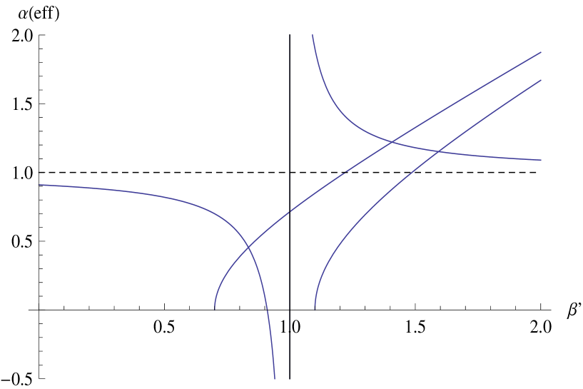
Figure 2: Graphical solution of (see Eq.(27)): $\displaystyle\alpha_{{\rm eff}}(\beta^{\prime})=\beta(\beta^{\prime})=\sqrt{\beta^{\prime 2}-K_{B}^{2}}$, with $\displaystyle K_{B}^{2}=\frac{2m}{\hbar^{2}}(2\mu B)$. There are either two solutions or just one depending on whether the value of $K_{B}$ (the onset of the hyperbola on the $\beta^{\prime}$ axis) is smaller or larger than $\beta_{c}^{\prime}$. In the figure we have plotted the solutions for two values that exemplify both cases. If $\displaystyle K_{B}\leq\beta_{c}^{\prime}$ there are two solutions, whereas if $K_{B}>\beta_{c}^{\prime}$ there is only one. Recall that in units of inverse length $\displaystyle\left[(\alpha_{1}+\alpha_{2})/2\right]$, in this plot $\beta^{\prime}_{c}=0.91$.

The full spectrum covers possibilities other than the one we have analysed. Both channels can be open, in which case the effective coupling in is no longer real; it is not difficult to repeat the calculations that led to (11) and find that it is the continuation of the function in (11) to complex arguments, $\displaystyle\alpha_{{\rm eq}}(-iK^{\prime})$, what appears here, in the situation of boundary conditions of a plane wave entering the $u$-channel. The physical interpretation is clear and reflects the fact that a fraction of the probability at the entrance leaks through the other channel, which is also open. As can be easily checked, the probability currents $J_{u}$ and $J_{v}$ are not separately conserved in the stationary state, but so is the sum of the two $J_{u}+J_{v}$ that involves the two components at once,

$$\frac{d}{dz}\left(J_{u}+J_{v}\right)=\frac{\hbar}{2im}\frac{d}{dz}\left(u^{*}(z)\frac{du(z)}{dz}-u(z)\frac{du^{*}(z)}{dz}+v^{*}(z)\frac{dv(z)}{dz}-v(z)\frac{dv^{*}(z)}{dz}\right)=0,$$ (25)

which expresses the conservation of the total probability current.

In our case of open $u$-channel and closed $v$-channel, the wavefunction $v(z)$ in (8) is real and its corresponding probability current $J_{v}=0$ vanishes, which prevents any probability leakage. It is the reason why $\displaystyle\alpha_{{\rm eff}}(\beta^{\prime})$ is real and why the probability conservation can be cast in terms of the $J_{u}$ alone.

Finally, let us briefly mention the possibility of discrete bound states for a given value of the magnetic field $B$, i.e., states with both $E\pm\mu B<0$ negative. They are the solutions of,

$$\alpha_{{\rm eff}}(\beta^{\prime})=\beta(\beta^{\prime})\equiv\sqrt{\beta^{\prime 2}-K_{B}^{2}},$$ (26)

with $\beta=-iK$ and $\beta^{\prime}=-iK^{\prime}$ in (4), and $\displaystyle K_{B}^{2}=\frac{2m}{\hbar^{2}}(2\mu B)$. With $\alpha_{1}\neq\alpha_{2}$, the number of solutions is either two or just one, depending on whether the value of $K_{B}$ is smaller or larger than $\beta_{c}^{\prime}$, respectively (see Fig. 2). In the limit of $K_{B}\gg\beta_{c}^{\prime}$, the intesect of the hyperbola and the curve $\alpha_{{\rm eff}}(\beta^{\prime})$ takes place for $\beta^{\prime}>K_{B}$, in the region where $\displaystyle\alpha_{{\rm eff}}(\beta^{\prime}>K_{B})\to\frac{\alpha_{1}+\alpha_{2}}{2}$ is asymptotically flat and the solution becomes,

$$E\approx-\mu B-\frac{\hbar^{2}}{2m}\left(\frac{\alpha_{1}+\alpha_{2}}{2}\right)^{2}.$$ (27)

3 Summary

We have presented a simple example in one dimension which consists of a spin 1/2 particle submitted to a delta-type potential that interatcs with different strength with the spin up and spin down components of the wavefuntion, and with an external magnetic field in the $x$-direction. Two coupled channels for scattering are available. We have checked that in the case of one open and one closed channels, with a suitable choice of the magnetic field a Feshbach resonance is produced so that in the neighbourhood of it the effective coupling flips sign, from attractive to repulsive. The reflection ceofficient is enormalously enhanced around it for all values of the incident wavenumber $K$, and the scattering phase shift is $\delta_{0}=\pi/2$.

4 Appendix

All the solutions presented in this article can be easily checked. We have essentially used the following two facts [6], namely,

$$\left(\frac{d^{2}}{dz^{2}}+k^{2}\right)\;\frac{e^{ik|z|}}{2ik}=\;\delta(z),\;\;\;\left(\frac{d^{2}}{dz^{2}}-\beta^{2}\right)\;\frac{e^{-\beta|z|}}{2\beta}=-\delta(z).$$ (28)

Let us briefly review the spectrum of a one-dimensional hamiltonian with an atractive delta-type potential:

$$-\frac{\hbar^{2}}{2m}\frac{d^{2}\chi(z)}{dz^{2}}-g\delta(z)\chi(z)=E\chi(z),$$ (29)

For $E>0$ it becomes,

$$\left(\frac{d^{2}}{dz^{2}}+k^{2}\right)\chi(z)=-2\alpha\chi(0)\delta(z),$$ (30)

where $\displaystyle\alpha=\frac{mg}{\hbar^{2}}$, and $\displaystyle k=\sqrt{\frac{2mE}{\hbar^{2}}}$. With scattering boundary condition of an entering plane wave plus an outgoing scattered wave, the solution, according to (28) is of the form,

$$\chi(z)=e^{ikz}-2\alpha\chi(0)\;\frac{e^{ik|z|}}{2ik},$$ (31)

where, self-consistently, one finds, $\displaystyle\chi(0)=-\frac{1}{\displaystyle 1+\frac{\alpha}{ik}}$, i.e.,

$$\chi(z)=e^{ikz}-\frac{\alpha}{ik+\alpha}e^{ik|z|}.$$ (32)

The reflection and transmission amplitudes $r(k)$, $t(k)$ defined as,

$$\chi(z\to-\infty)\sim e^{ikz}+r(k)e^{-ikz},$$

$$\chi(z\to+\infty)\sim t(k)e^{ikz},$$ (33)

can be read off immediately,

$$r(k)=-\frac{\alpha}{ik+\alpha},\;\;\;t(k)=\frac{ik}{ik+\alpha}.$$ (34)

If $E<0$ this potential always holds only one bound state. Eq. (29) becomes, with $\displaystyle\beta=\sqrt{\frac{2m|E|}{\hbar^{2}}}$,

$$\left(\frac{d^{2}}{dz^{2}}-\beta^{2}\right)\chi(z)=-2\alpha\chi(0)\delta(z),$$ (35)

and according to (28),

$$\chi(z)=\frac{\alpha}{\beta}\chi(0)\;e^{-\beta|z|}.$$ (36)

Setting $z=0$ one is led to conclude that

$$\beta=\alpha,$$ (37)

which is the quantization condition for the bound state energy $\displaystyle E=-\frac{\hbar^{2}}{2m}\alpha^{2}$, whereas $\chi(0)$ remains free for normalization of the wave function:

$$\chi(z)=\sqrt{\alpha}\;e^{-\alpha|z|}.$$ (38)

The wave function of the bound state extends over a distance $1/\alpha$ around $z=0$.

5 Acknowledgments

We thank Prof. Nuria Barberán for reading the manuscript and for helpful discussions and comments. We acknowledge financial support by the Spanish Government through the Consolider CPAN project CSD2007-00042, and by the Generalitat de Catalunya Program under contract number 2009SGR502.

References

[1] Feshbach, H., Ann. Phys. 5, 357 (1958);
Ann. Phys. 19, 287 (1962).
[2] Fano, U., Phys. Rev. 124, 1866 (1961)
[3]Advances in Atomic Physics, part 6, C. Cohen- Tannoudji,
D. Guéry-Odelin, (World Scientific, 2011)
[4]Atom-Atom Interactions in Ultracold Quantum Gases,
Claude Cohen-Tannoudji course (Bilbao, 28 and 28 May 2007).