Subbarrier fusion reactions and many-particle quantum tunneling

Abstract

Low energy heavy-ion fusion reactions are governed by quantum tunneling through the Coulomb barrier formed by a strong cancellation of the repulsive Coulomb force with the attractive nuclear interaction between the colliding nuclei. Extensive experimental as well as theoretical studies have revealed that fusion reactions are strongly influenced by couplings of the relative motion of the colliding nuclei to several nuclear intrinsic motions. Heavy-ion subbarrier fusion reactions thus provide a good opportunity to address a general problem on quantum tunneling in the presence of couplings, which has been a popular subject in the past decades in many branches of physics and chemistry. Here we review theoretical aspects of heavy-ion subbarrier fusion reactions from the view point of quantum tunneling in systems with many degrees of freedom. Particular emphases are put on the coupled-channels approach to fusion reactions, and the barrier distribution representation for multi-channel penetrability. We also discuss an application of the barrier distribution method to elucidation of the mechanism of dissociative adsorption of H₂ molecules in surface science.

1 Introduction

Quantum mechanics is indispensable in understanding microscopic systems such as atoms, molecules, and atomic nuclei. One of its fundamental aspects is a quantum tunneling, where a particle penetrates into a classically forbidden region. This is a wave phenomenon and is frequently encountered in diverse processes in physics and chemistry.

The importance of quantum tunneling has been recognized from the birth of quantum mechanics. For instance, it was as early as 1928 when Gamow, and independently Gurney and Condon, applied quantum tunneling to $\alpha$ decays of atomic nuclei and successfully explained the systematics of the experimental half-lives of radioactive nuclei[1, 2].

In many applications of quantum tunneling, one only considers penetration of a one-dimensional potential barrier, or a barrier with a single variable. In general, however, a particle which penetrates a potential barrier is never isolated but interacts with its surroundings or environments, resulting in modification in its behavior. Moreover, when the particle is a composite particle, the quantum tunneling has to be discussed from a many-particle point of view. Quantum tunneling therefore inevitably takes place in reality in a multi-dimensional space. Such problem was first addressed by Kapur and Peierls in 1937 [3]. Their theory has further been developed by e.g., Banks, Bender, and Wu [4], Gervais and Sakita [5], Brink, Nemes, and Vautherin [6], Schmid [7], and Takada and Nakamura [8].

When the quantum tunneling occurs in a complex system, such as the trapped flux in a superconducting quantum interference devices (SQUID) ring [9], the tunneling variable couples to a large number of other degrees of freedom. In such systems, the environmental degrees of freedom more or less reveal a dissipative character. Quantum tunneling under the influence of dissipative environments plays an important role and is a fundamental problem in many fields of physics and chemistry. This problem has been studied in detail by Caldeira and Leggett [10]. This seminal work has stimulated lots of experimental and theoretical works, and has made quantum tunneling in systems with many degrees of freedom a topic of immense interest during the past decades [11].

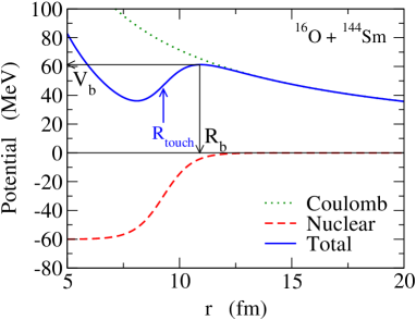
Figure 1: The internucleus potential between ¹⁶O and ¹⁴⁴Sm nuclei as a function of the relative distance. The dotted and the dashed lines are the Coulomb and the nuclear potentials, respectively, while the solid line denotes the total potential. $V_{b}$ and $R_{b}$ are the height and the position of the Coulomb barrier, respectively. $R_{\rm touch}$ is the touching radius at which the projectile and the target nuclei start overlapping significantly with each other.

In nuclear physics, one of the typical examples of tunneling phenomena is heavy-ion fusion reaction at energies near and below the Coulomb barrier[12, 13]. Fusion is defined as a reaction in which two separate nuclei combine together to form a compound nucleus. In order for fusion reaction to take place, the relative motion between the colliding nuclei has to overcome the Coulomb barrier formed by a strong cancellation between the long-ranged repulsive Coulomb and the short-ranged attractive nuclear forces (as a typical example, Fig.1 shows the internucleus potential between ¹⁶O and ¹⁴⁴Sm nuclei as a function of the relative distance). Unless under extreme conditions, it is reasonable to assume that atomic nuclei are isolated systems and the couplings to external environments can be neglected. Nevertheless, one can still consider intrinsic environments. The whole spectra of excited states of the target and projectile nuclei (as well as several sorts of nucleon transfer processes) are populated in a complex way during fusion reactions. They act as environments to which the relative motion between the colliding nuclei couples. In fact, it has by now been well established that cross sections of heavy-ion fusion reactions are substantially enhanced due to couplings to nuclear intrinsic degrees of freedom at energies below the Coulomb barrier as compared to the predictions of a simple potential model [12, 13, 14, 15, 16, 17, 18]. Heavy-ion subbarrier fusion reactions thus make good examples of environment-assisted tunneling phenomena.

Theoretically the standard way to address the effects of the couplings between the relative motion and nuclear intrinsic degrees of freedom on fusion reactions is to numerically solve the coupled-channels equations which include all the relevant channels. In the eigen-channel representation of coupled-channels equations, the channel coupling effects can be interpreted in terms of a distribution of fusion barriers[13, 19, 20, 21]. In this representation, the fusion cross section is given by a weighted sum of the fusion cross sections for each eigen-barrier. Those eigen-barriers lower than the original barrier are responsible for the enhancement of the fusion cross section at energies below the Coulomb barrier. Based on this idea, Rowley, Satchler, and Stelson have proposed a method to extract barrier distributions directly from experimental fusion excitation functions by taking the second derivative of the product of the fusion cross section and the center of mass energy $E\sigma_{\rm fus}$ with respect to $E$, i.e., $d^{2}(E\sigma_{\rm fus})/dE^{2}$  [22]. This method was tested against high precision experimental data of fusion cross sections soon after the method was proposed[23]. The extracted fusion barrier distributions were sensitive to the effects of channel-couplings and provided a much more apparent way of understanding their effects on the fusion process than the fusion excitation functions themselves. It is now well recognised that the barrier distribution approach is a standard tool for heavy-ion subbarrier fusion reactions [13, 18].

The aim of this paper is to review theoretical aspects of heavy-ion subbarrier fusion reactions from the view point of quantum tunneling of composite particles. To this end, we mainly base our discussions on the coupled-channels approach. Earlier reviews on the subbarrier fusion reactions can be found in Refs. BT98,DHRS98,B88,SRB86,R94. See also Refs. CGDH06 and LS05 for reviews on subbarrier fusion reactions of radioactive nuclei, and e.g., Refs. A00 and AM12 for reviews on fusion reactions relevant to synthesis of superheavy elements, both of which we do not cover in this article.

The paper is organized as follows. We will first discuss in the next section a potential model approach to heavy-ion fusion reactions. This is the simplest approach to fusion reaction, in which only elastic scattering and fusion are assumed to occur. This approach is adequate for light systems, but for fusion with a medium-heavy or heavy target nucleus the effects of nuclear excitations during fusion start playing an important role. In Sec. 3, we will discuss such nuclear structure effect on heavy-ion fusion reactions. To this end, we will introduce and detail the coupled-channels formalism which takes into account the inelastic scattering and transfer processes during fusion reactions. In Sec. 4, light will be shed on the fusion barrier distribution representation of fusion cross section defined as $d^{2}(E\sigma_{\rm fus})/dE^{2}$. It has been known that this approach is exact when the excitation energy of the intrinsic motion is zero, but we will demonstrate that one can generalize it unambiguously using the eigen-channel approach also to the case when the excitation energy is finite. In Sec. 5, we will turn to a discussion on the present status of our understanding of deep subbarrier fusion reactions. At these energies, fusion cross sections have been shown to be suppressed compared to the values of the standard coupled-channels calculations. This phenomenon may be related to dissipative quantum tunneling, that is, an irreversible coupling to intrinsic degrees of freedom. In Sec. 6, we discuss an application of the barrier distribution method to surface physics, more specifically, the effect of rotational excitations on a dissociative adsorption process of H₂ molecules. We then summarize the paper in Sec. 7.

2 One dimensional potential model

2.1 Ion-ion potential

Theoretically, the simplest approach to heavy-ion fusion reactions is to use the one dimensional potential model where both the projectile and the target are assumed to be structureless. A potential between the projectile and the target is given by a function of the relative distance $r$ between them. It consists of two parts, that is,

$$V(r)=V_{N}(r)+V_{C}(r),$$ (1)

where $V_{N}(r)$ is the nuclear potential, and $V_{C}(r)$ is the Coulomb potential given by

$$V_{C}(r)=\frac{Z_{P}Z_{T}e^{2}}{r},$$ (2)

in the outside region where the projectile and the target nuclei do not significantly overlap with each other. Figure 1 shows a typical potential $V(r)$ for the $s$-wave scattering of the ¹⁶O + ¹⁴⁴Sm reaction. The dotted and the dashed lines are the nuclear and the Coulomb potentials, respectively, while the total potential $V(r)$ is denoted by the solid line. One can see that a potential barrier appears due to a strong cancellation between the short-ranged attractive nuclear interaction and the long-ranged repulsive Coulomb force. This potential barrier is referred to as the Coulomb barrier and has to be overcome in order for the fusion reaction to take place. $R_{\rm touch}$ in the figure is the touching radius, at which the projectile and the target nuclei begin overlapping considerably. One can see that the Coulomb barrier is located outside the touching radius.

There are several ways to estimate the nuclear potential $V_{N}(r)$. One standard method is to fold a nucleon-nucleon interaction with the projectile and the target densities [28]. The direct part of the nuclear potential in this double folding procedure is given by

$$V_{N}(r)=\int d\mbox{\boldmath$r$}_{1}d\mbox{\boldmath$r$}_{2}\,v_{NN}(\mbox{\boldmath$r$}_{2}-\mbox{\boldmath$r$}_{1}-\mbox{\boldmath$r$})\rho_{P}(\mbox{\boldmath$r$}_{1})\rho_{T}(\mbox{\boldmath$r$}_{2}),$$ (3)

where $v_{NN}$ is an effective nucleon-nucleon interaction, and $\rho_{P}$ and $\rho_{T}$ are the densities of the projectile and the target, respectively. The double-folding potential is in general a non-local potential due to the anti-symmetrization effect of nucleons. Usually, either a zero-range approximation [28, 29] or a local momentum approximation [30, 31, 32, 33, 34] is employed in order to treat the non-locality of the potential.

A phenomenological nuclear potential has also been employed. For instance, a Woods-Saxon form

$$V_{N}(r)=-\frac{V_{0}}{1+\exp[(r-R_{0})/a]},$$ (4)

with

$$V_{0} = 16\pi\gamma\bar{R}a,$$ (5)

$$R_{0} = R_{P}+R_{T},$$ (6)

$$R_{i} = 1.20A_{i}^{1/3}-0.09~{}{\rm fm}~{}~{}~{}~{}~{}~{}(i=P,T),$$ (7)

$$\bar{R} = R_{P}R_{T}/(R_{P}+R_{T}),$$ (8)

$$\gamma = 0.95\left[1-1.8\left(\frac{N_{P}-Z_{P}}{A_{P}}\right)\left(\frac{N_{T}-Z_{T}}{A_{T}}\right)\right]~{}{\rm MeV~{}fm^{-2}},$$ (9)

$$1/a = 1.17\left[1+0.53\left(A_{P}^{-1/3}+A_{T}^{-1/3}\right)\right]~{}{\rm fm^{-1}},$$ (10)

has been widely used, where the parameters were determined from a least-squares fit to the experimental data of heavy-ion elastic scattering [35, 36].

A nuclear potential so constructed has been successful in reproducing experimental angular distributions of elastic and inelastic scattering for many systems. Moreover, the empirical value of surface diffuseness parameter, $a\sim$ 0.63 fm, is consistent with a double folding potential. Recently, a value of the surface diffuseness parameter has been determined unambiguously using heavy-ion quasi-elastic scattering at deep subbarrier energies[37, 38]. It has been confirmed that the experimental data are consistent with a value around $a\sim$ 0.63 fm [38, 39, 40, 41].

In marked contrast, recent experimental data for heavy-ion subbarrier fusion reactions suggest that a much larger value of diffuseness, ranging from 0.75 to 1.5 fm, is required to fit the data [18, 42, 43, 44, 45, 46]. The Woods-Saxon potential which fits elastic scattering overestimates fusion cross sections at energies both above and below the Coulomb barrier, having an inconsistent energy dependence with the experimental fusion excitation function. A reason for the large discrepancies in diffuseness parameters extracted from scattering and fusion analyses has not yet been fully understood. However, it is probably the case that the double folding procedure is valid only in the surface region, while several dynamical effects come into play in the inner part where fusion is sensitive to.

We summarize the relation between the surface diffuseness parameter $a$ of a nuclear potential and the parameters of the Coulomb barrier, that is, the curvature, the barrier height, and the barrier position in Appendix A for an exponential and a Woods-Saxon potentials.

2.2 Fusion cross sections

In the potential model, the internucleus potential, $V(r)$, is supplemented by an imaginary part, $-iW(r)$, which mocks up the formation of a compound nucleus. One then solves the Schrödinger equation

$$\left[-\frac{\hbar^{2}}{2\mu}\frac{d^{2}}{dr^{2}}+V(r)-iW(r)+\frac{l(l+1)\hbar^{2}}{2\mu r^{2}}-E\right]u_{l}(r)=0,$$ (11)

for each partial wave $l$, where $\mu$ is the reduced mass of the system, with the boundary conditions of

$$u_{l}(r) \sim r^{l+1}~{}~{}~{}~{}~{}~{}~{}~{}~{}~{}~{}~{}~{}~{}~{}~{}~{}~{}~{}~{}~{}~{}~{}~{}~{}~{}~{}~{}~{}~{}~{}r\to 0,$$ (12)

$$= H_{l}^{(-)}(kr)-S_{l}\,H_{l}^{(+)}(kr)~{}~{}~{}~{}~{}~{}r\to\infty.$$ (13)

Here, $H_{l}^{(+)}$ and $H_{l}^{(-)}$ are the outgoing and the incoming Coulomb wave functions, respectively. $S_{l}$ is the nuclear $S$-matrix, and $k=\sqrt{2\mu E/\hbar^{2}}$ is the wave number associated with the energy $E$.

If the imaginary part of the potential, $W(r)$, is confined well inside the Coulomb barrier, one can regard the total absorption cross section as fusion cross section, i.e.,

$$\sigma_{\rm fus}(E)\sim\sigma_{\rm abs}(E)=\frac{\pi}{k^{2}}\sum_{l}(2l+1)\left(1-|S_{l}|^{2}\right).$$ (14)

In heavy-ion fusion reactions, instead of imposing the regular boundary condition at the origin, Eq. (12), the so called incoming wave boundary condition (IWBC) is often applied without introducing the imaginary part of the potential, $W(r)$ [19, 47]. Under the incoming wave boundary condition, the wave function has a form

$$u_{l}(r)=\sqrt{\frac{k}{k_{l}(r)}}\,{\cal T}_{l}\exp\left(-i\int^{r}_{r_{\rm abs}}k_{l}(r^{\prime})dr^{\prime}\right)~{}~{}~{}~{}~{}r\leq r_{\rm abs},$$ (15)

at the distance smaller than the absorption radius $r_{\rm abs}$, which is taken to be inside the Coulomb barrier. Here, $k_{l}(r)$ is the local wave number for the $l$-th partial wave defined by

$$k_{l}(r)=\sqrt{\frac{2\mu}{\hbar^{2}}\left(E-V(r)-\frac{l(l+1)\hbar^{2}}{2\mu r^{2}}\right)}.$$ (16)

The incoming wave boundary condition corresponds to the case where there is a strong absorption in the inner region so that the incoming flux never returns back. For heavy-ion fusion reactions, the final result is not sensitive to the choice of the absorption radius $r_{\rm abs}$, and it is often taken to be at the pocket of the potential[48]. With the incoming wave boundary condition, ${\cal T}_{l}$ in Eq. (15) is interpreted as the transmission coefficient. Equation (14) is then transformed to

$$\sigma_{\rm fus}(E)=\frac{\pi}{k^{2}}\sum_{l}(2l+1)P_{l}(E),$$ (17)

where $P_{l}(E)$ is the penetrability for the $l$-wave scattering defined as

$$P_{l}(E)=1-|S_{l}|^{2}=\left|{\cal T}_{l}\right|^{2},$$ (18)

for the boundary conditions (13) and (15). The mean angular momentum of the compound nucleus is evaluated in a similar way as

$$\langle l\rangle(E)=\frac{\frac{\pi}{k^{2}}\sum_{l}l(2l+1)P_{l}(E)}{\frac{\pi}{k^{2}}\sum_{l}(2l+1)P_{l}(E)}.$$ (19)

For a parabolic potential, Wong has derived an analytic expression for fusion cross sections, Eq. (17)[49]. We will discuss it in Appendix B.

The incoming wave boundary condition, Eq. (15), has two advantages over the regular boundary condition, Eq. (12). The first advantage is that the imaginary part of nuclear potential is not needed, and the number of adjustable parameters can be reduced. The second point is that the incoming wave boundary condition directly provides the penetrability $P_{l}(E)=\left|{\cal T}_{l}\right|^{2}$ and thus the round off error can be avoided in evaluating $1-|S_{l}|^{2}$. This is a crucial point at energies well below the Coulomb barrier, where $S_{l}$ is close to unity. Notice that the incoming wave boundary condition does not necessarily correspond to the limit of $W(r)\to\infty$, as the quantum reflection due to $W(r)$ has to be neglected in order to realize it. The incoming wave boundary condition should thus be regarded as a different model from the regular boundary condition.

2.3 Comparison with experimental data: success and failure of the potential model

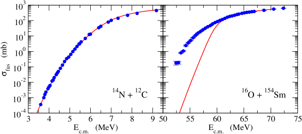
Figure 2: Comparison of experimental fusion cross sections for the ¹⁴N+¹²C system (the left panel) and ¹⁶O+¹⁵⁴Sm system (the right panel) with results of the potential model calculations (the solid line). The height of the Coulomb barrier is around $V_{b}\sim$ 6.9 MeV and 59 MeV for ¹⁴N+¹²C and ¹⁶O+¹⁵⁴Sm, respectively. The experimental data are taken from Refs. SSW77 and LDH95 for the ¹⁴N+¹²C and the ¹⁶O+¹⁵⁴Sm reactions, respectively.

Let us now compare the one dimensional potential model for heavy-ion fusion reaction with experimental data. Figure 2 shows the experimental excitation functions of fusion cross section for ¹⁴N+¹²C (the left panel) and ¹⁶O+¹⁵⁴Sm (the right panel) systems, as well as results of the potential model calculation (the solid lines). One can see that the potential model well reproduces the experimental data for the lighter system, ¹⁴N + ¹²C. On the other hand, the potential model apparently underestimates fusion cross sections for the heavier system, ¹⁶O + ¹⁵⁴Sm, although it reproduces the experimental data at energies above the Coulomb barrier, which is about 59 MeV for this system.

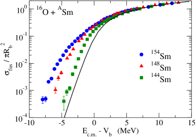
Figure 3: The experimental fusion cross sections for ¹⁶O+^144,148,154Sm systems, taken from Ref. LDH95. In order to remove the trivial target dependence, the experimental fusion cross sections are divided by $\pi R_{b}^{2}$, where $R_{b}$ is the position of the Coulomb barrier, and the energies are measured with respect to the barrier height, $V_{b}$, for each system. The solid line shows the result of the potential model calculation.

In order to understand the origin for the failure of the potential model, Fig. 3 shows the experimental fusion excitation functions for ¹⁶O + ^144,148,154Sm reactions [18] and a comparison with the potential model (the solid line). To remove trivial target dependence, these are plotted as a function of center of mass energy relative to the barrier height for each system, and the fusion cross sections are divided by the geometrical factor, $\pi R_{b}^{2}$. With these prescriptions, the fusion cross sections for the different systems are matched with each other at energies above the Coulomb barrier, although one can also consider a more refined prescription[51, 52]. The barrier height and the result of the potential model are obtained with the Akyüz-Winther potential[36]. One again observes that the experimental fusion cross sections are drastically enhanced at energies below the Coulomb barrier compared with the prediction of the potential model. Moreover, one also observes that the degree of enhancement of fusion cross section depends strongly on the target nucleus. That is, the enhancement for the ¹⁶O + ¹⁵⁴Sm system is order of magnitude, while that for the ¹⁶O + ¹⁴⁴Sm system is about a factor of four at energies below the Coulomb barrier. This strong target dependence of fusion cross sections suggests that low-lying collective excitations play a role, as we will discuss in the next section.

The inadequacy of the potential model has been demonstrated in a more transparent way by Balantekin et al.[53]. Within the semi-classical approximation, the penetrability for a one-dimensional barrier can be inverted to yield the barrier thickness [54]. Balantekin et al. applied such inversion formula directly to the experimental fusion cross sections in order to construct an effective internucleus potential. Assuming a one-dimensional energy-independent local potential, the resultant potentials were unphysically thin for heavy systems, often multi-valued potential. This result was confirmed also by the systematic study in Ref. IK84. These analyses have provided a clear evidence for the inadequacy of the one-dimensional barrier passing model for heavy-ion fusion reactions, and has triggered to develop the coupled-channels approach, which we will discuss in the next section.

In passing, we have recently applied the inversion procedure in a modified way to determine the lowest potential barrier among the distributed ones due to the effects of channel coupling [56]. The extracted potential for the ¹⁶O + ²⁰⁸Pb scattering is well behaved, indicating that the channel coupling indeed plays an essential role in subbarrier fusion reactions.

3 Coupled-channels formalism for heavy-ion fusion reactions

3.1 Nuclear structure effects on subbarrier fusion reactions

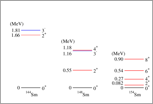
Figure 4: The experimental low-lying spectra of ^144,148,154Sm nuclei.

The strong target dependence of subbarrier fusion cross sections shown in Fig. 3 suggests that the enhancement of fusion cross sections is due to low-lying collective excitations of the colliding nuclei during fusion. The low-lying excited states in even-even nuclei are collective states, and strongly reflect the pairing correlation and shell structure. They have thus strongly coupled to the ground state, and also have a strong mass number and atomic number dependences. As an example, the low-lying spectra are shown in Fig. 4 for ^144,148,154Sm. The ¹⁴⁴Sm nucleus is close to the (sub-)shell closures ($Z$=64 and $N=82$) and is characterized by a strong octupole vibration. ¹⁵⁴Sm, on the other hand, is a well deformed nucleus, and has a well developed ground state rotational band. ¹⁴⁸Sm is a transitional nucleus, and there exists a soft quadrupole vibration in the low-lying spectrum. One can clearly see that there is a strong correlation between the degree of enhancement of fusion cross sections shown in Fig. 3 and e.g., the energy of the first 2⁺ state.

Besides the low-lying collective excitations, there are many other modes of excitations in atomic nuclei. Among them, non-collective excitations couple only weakly to the ground state and usually they do not affect in a significant way heavy-ion fusion reactions, even though the number of non-collective states is large[57]. Couplings to giant resonances are relatively strong due to their collective character. However, since their excitation energies are relatively large and also are smooth functions of mass number [58, 59, 60], their effects can be effectively incorporated in a choice of internuclear potential through the adiabatic potential normalization (see the next section).

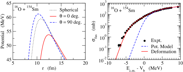
Figure 5: (The left panel) the orientation dependence of fusion potential for the ¹⁶O+¹⁵⁴Sm reaction. The solid and the dashed lines are the potentials when the orientation of the deformed ¹⁵⁴Sm target is $\theta=$ 0 and $\pi/2$, respectively. The dotted line denotes the potential when the deformation of ¹⁵⁴Sm is not taken into account. (The right panel) the fusion cross sections for the ¹⁶O+¹⁵⁴Sm reaction. The dashed line is the result of the potential model calculation shown in Fig. 3, while the solid line is obtained by taking into account the deformation of the ¹⁵⁴Sm nucleus with Eq. (20). The experimental data are taken from Ref. LDH95.

The effect of rotational excitations of a heavy deformed nucleus can be easily taken into account using the orientation average formula[21, 49, 17, 61, 62, 63]. For an axially symmetric target nucleus, fusion cross sections are computed with this formula as,

$$\sigma_{\rm fus}(E)=\int^{1}_{0}d(\cos\theta)\,\sigma_{\rm fus}(E;\theta),$$ (20)

where $\theta$ is the angle between the symmetry axis and the beam direction. $\sigma_{\rm fus}(E;\theta)$ is a fusion cross section for a fixed orientation angle, $\theta$. This is obtained with e.g., a deformed Woods-Saxon potential,

$$V_{N}(r,\theta)=-\frac{V_{0}}{1+\exp[(r-R_{0}-R_{T}\beta_{2}Y_{20}(\theta)-R_{T}\beta_{4}Y_{40}(\theta))/a]},$$ (21)

which can be constructed by changing the target radius $R_{T}$ in the Woods-Saxon potential, Eq. (4), to $R_{T}\to R_{T}(1+\beta_{2}Y_{20}(\theta)+\beta_{4}Y_{40}(\theta))$. See Ref. AHNC12 for a recent application of this formula to fusion of massive systems, in which the formula is combined with classical Langevin calculations.

The left panel of Fig. 5 shows the potential for the ¹⁶O+¹⁵⁴Sm reaction obtained with the deformation parameters of $\beta_{2}$=0.306 and $\beta_{4}=0.05$. The deformation of the Coulomb potential is also taken into account (see Sec. 3.4 for details). The solid line shows the potential for $\theta=0$. For this orientation angle, the potential is lowered by the deformation effect as compared to the spherical potential shown by the dotted line, because the attractive nuclear interaction is active from relatively large values of $r$. The opposite happens when $\theta=\pi/2$ as shown by the dashed line. The potential is distributed between the solid and the dashed lines according to the value of orientation angle, $\theta$. The solid line in the right panel of Fig. 5 shows the fusion cross sections obtained by averaging the contribution of all the orientation angles through Eq. (20). Since the tunneling probability has an exponentially strong dependence on the barrier height, the fusion cross sections are significantly enhanced for those orientations which yield a lower barrier than the spherical case. It is remarkable that this simple calculation accounts well for the experimental enhancement of fusion cross sections at subbarrier energies. Evidently, nuclear structure effects significantly enhance fusion cross sections at energies below the Coulomb barrier, which make fusion reactions an interesting probe for nuclear structure.

3.2 Coupled-channels equations with full angular momentum coupling

The nuclear structure effects can be taken into account in a more quantal way using the coupled-channels method. In order to formulate the coupled-channels method, consider a collision between two nuclei in the presence of the coupling of the relative motion, $\mbox{\boldmath$r$}=(r,\hat{\mbox{\boldmath$r$}})$, to a nuclear intrinsic motion $\xi$. We assume the following Hamiltonian for this system,

$$H(\mbox{\boldmath$r$},\xi)=-\frac{\hbar^{2}}{2\mu}\nabla^{2}+V(r)+H_{0}(\xi)+V_{\rm coup}(\mbox{\boldmath$r$},\xi),$$ (22)

where $H_{0}(\xi)$ and $V_{\rm coup}(\mbox{\boldmath$r$},\xi)$ are the intrinsic and the coupling Hamiltonians, respectively. In general the intrinsic degree of freedom $\xi$ has a finite spin. We therefore expand the coupling Hamiltonian in multipoles as

$$V_{\rm coup}(\mbox{\boldmath$r$},\xi)=\sum_{\lambda>0}f_{\lambda}(r)Y_{\lambda}(\hat{\mbox{\boldmath$r$}})\cdot T_{\lambda}(\xi).$$ (23)

Here $Y_{\lambda}(\hat{\mbox{\boldmath$r$}})$ are the spherical harmonics and $T_{\lambda}(\xi)$ are spherical tensors constructed from the intrinsic coordinate. The dot indicates a scalar product. The sum is taken over all values of $\lambda$ except for $\lambda=0$, which is already included in the bare potential, $V(r)$.

For a given total angular momentum $J$ and its $z$ component $M$, one can define the channel wave functions as

$$\langle\hat{\mbox{\boldmath$r$}}\xi|(\alpha lI)JM\rangle=\sum_{m_{l},m_{I}}\langle lm_{l}Im_{I}|JM\rangle Y_{lm_{l}}(\hat{\mbox{\boldmath$r$}})\varphi_{\alpha Im_{I}}(\xi),$$ (24)

where $l$ and $I$ are the orbital and the intrinsic angular momenta, respectively. $\varphi_{\alpha Im_{I}}(\xi)$ are the wave functions of the intrinsic motion which obey

$$H_{0}(\xi)\varphi_{\alpha Im_{I}}(\xi)=\epsilon_{\alpha I}\,\varphi_{\alpha Im_{I}}(\xi).$$ (25)

Here, $\alpha$ denotes any quantum number besides the angular momentum. Expanding the total wave function with the channel wave functions as

$$\Psi_{J}(\mbox{\boldmath$r$},\xi)=\sum_{\alpha,l,I}\frac{u^{J}_{\alpha lI}(r)}{r}\langle\hat{\mbox{\boldmath$r$}}\xi|(\alpha lI)JM\rangle,$$ (26)

the coupled-channels equations for $u^{J}_{\alpha lI}(r)$ read

$$\left[-\frac{\hbar^{2}}{2\mu}\frac{d^{2}}{dr^{2}}+\frac{l(l+1)\hbar^{2}}{2\mu r^{2}}+V(r)-E+\epsilon_{\alpha I}\right]u^{J}_{\alpha lI}(r)+\sum_{\alpha^{\prime},l^{\prime},I^{\prime}}V^{J}_{\alpha lI;\alpha^{\prime}l^{\prime}I^{\prime}}(r)u^{J}_{\alpha^{\prime}l^{\prime}I^{\prime}}(r)=0,$$ (27)

where the coupling matrix elements $V^{J}_{\alpha lI;\alpha^{\prime}l^{\prime}I^{\prime}}(r)$ are given as [65]

$$V^{J}_{\alpha lI;\alpha^{\prime}l^{\prime}I^{\prime}}(r) = \langle(\alpha lI)JM|V_{\rm coup}(\mbox{\boldmath$r$},\xi)|(\alpha^{\prime}l^{\prime}I^{\prime})JM\rangle,$$ (31)

$$= \sum_{\lambda}(-)^{I-I^{\prime}+l^{\prime}+J}f_{\lambda}(r)\langle l||Y_{\lambda}||l^{\prime}\rangle\langle\alpha I||T_{\lambda}||\alpha^{\prime}I^{\prime}\rangle$$

$$\times\sqrt{(2l+1)(2I+1)}\left\{\begin{array}[]{ccc}I^{\prime}&l^{\prime}&J\\ l&I&\lambda\end{array}\right\}.$$

Notice that these matrix elements are independent of $M$.

For the sake of simplicity of the notation, in the following let us introduce a simplified notation, $n=\{\alpha,l,I\}$, and suppress the index $J$. The coupled-channels equation (27) then reads,

$$\left[-\frac{\hbar^{2}}{2\mu}\frac{d^{2}}{dr^{2}}+\frac{l_{n}(l_{n}+1)\hbar^{2}}{2\mu r^{2}}+V(r)-E+\epsilon_{n}\right]u_{n}(r)+\sum_{n^{\prime}}V_{nn^{\prime}}(r)u_{n^{\prime}}(r)=0.$$ (32)

These coupled-channels equations are solved with the incoming wave boundary conditions of

$$u_{n}(r) \sim \sqrt{\frac{k_{n_{i}}}{k_{n}(r)}}\,{\cal T}^{J}_{nn_{i}}\exp\left(-i\int^{r}_{r_{\rm abs}}k_{n}(r^{\prime})dr^{\prime}\right)~{}~{}~{}~{}~{}~{}~{}~{}~{}~{}~{}~{}~{}~{}~{}~{}r\leq r_{\rm abs},$$ (33)

$$= H_{l_{n}}^{(-)}(k_{n}r)\delta_{n,n_{i}}-\sqrt{\frac{k_{n_{i}}}{k_{n}}}\,{\cal S}^{J}_{nn_{i}}H_{l_{n}}^{(+)}(k_{n}r)~{}~{}~{}~{}~{}~{}~{}~{}~{}~{}~{}~{}~{}~{}r\to\infty,$$ (34)

where $n_{i}$ denotes the entrance channel. The local wave number $k_{n}(r)$ is defined by

$$k_{n}(r)=\sqrt{\frac{2\mu}{\hbar^{2}}\left(E-\epsilon_{n}-\frac{l_{n}(l_{n}+1)\hbar^{2}}{2\mu r^{2}}-V(r)\right)},$$ (35)

whereas $k_{n}=k_{n}(r=\infty)=\sqrt{2\mu(E-\epsilon_{n})/\hbar^{2}}$. Once the transmission coefficients ${\cal T}^{J}_{nn_{i}}$ are obtained, the inclusive penetrability of the Coulomb potential barrier is given by

$$P_{J}(E)=\sum_{n}|{\cal T}^{J}_{nn_{i}}|^{2}.$$ (36)

The fusion cross section is then given by

$$\sigma_{\rm fus}(E)=\frac{\pi}{k^{2}}\sum_{J}(2J+1)P_{J}(E),$$ (37)

where we have assumed that the initial intrinsic state has spin zero, $I_{i}=0$. This equation for fusion cross section is similar to Eq. (17) except that the penetrability $P_{J}(E)$ is now influenced by the channel coupling effects.

3.3 Iso-centrifugal approximation

The full coupled-channels calculations (32) quickly become intricate if many physical channels are included. The dimension of the resulting coupled-channels problem is in general too large for practical purposes. For this reason, the iso-centrifugal approximation, which is sometimes referred to as the no-Coriolis approximation or the rotating frame approximation, has often been introduced [21, 48, 63, 66, 67, 68, 69, 70]. In the iso-centrifugal approximation to the coupled-channels equations, Eq. (32), one first replaces the angular momentum of the relative motion in each channel by the total angular momentum $J$, that is,

$$\frac{l_{n}(l_{n}+1)\hbar^{2}}{2\mu r^{2}}\approx\frac{J(J+1)\hbar^{2}}{2\mu r^{2}}.$$ (38)

This corresponds to assuming that the change in the orbital angular momentum due to the excitation of the intrinsic degree of freedom is negligible. Introducing the weighted average wave function

$$\bar{u}_{I}(r)=(-)^{I}\sum_{l}\langle J0I0|l0\rangle u_{lI}(r),$$ (39)

where we have suppressed the index $\alpha$ for simplicity, and using the relation

$$\sum_{l}(-)^{l^{\prime}+J+\lambda}\sqrt{2l+1}\left\{\begin{array}[]{ccc}J&I&l\\ \lambda&l^{\prime}&I^{\prime}\\ \end{array}\right\}\langle l0\lambda 0|l^{\prime}0\rangle\langle J0I0|l0\rangle=\frac{(-)^{I^{\prime}}}{\sqrt{2I+1}}\langle J0I^{\prime}0|l^{\prime}0\rangle\langle I^{\prime}0\lambda 0|I0\rangle,$$ (40)

one finds that the wave function $\bar{u}_{I}(r)$ obeys the reduced coupled-channels equations,

$$\left(-\frac{\hbar^{2}}{2\mu}\frac{d^{2}}{dr^{2}}+\frac{J(J+1)\hbar^{2}}{2\mu r^{2}}+V(r)-E+\epsilon_{I}\right)\bar{u}_{I}(r)+\sum_{I^{\prime}}\sum_{\lambda}\sqrt{\frac{2\lambda+1}{4\pi}}f_{\lambda}(r)\langle\varphi_{I0}|T_{\lambda 0}|\varphi_{I^{\prime}0}\rangle\bar{u}_{I^{\prime}}(r)=0.$$ (41)

These are nothing but the coupled-channels equations for a spin-zero system with the interaction Hamiltonian given by

$$V_{\rm coup}=\sum_{\lambda}f_{\lambda}(r)Y_{\lambda}(\hat{\mbox{\boldmath$r$}}=0)\cdot T_{\lambda}=\sum_{\lambda}\sqrt{\frac{2\lambda+1}{4\pi}}f_{\lambda}(r)T_{\lambda 0}.$$ (42)

In solving the reduced coupled-channels equations, similar boundary conditions are imposed for $\bar{u}_{I}$ as those for $u_{lI}$,

$$\bar{u}_{I}(r) \sim \sqrt{\frac{k_{I_{i}}}{k_{I}(r)}}\,\bar{{\cal T}}^{J}_{II_{i}}\exp\left(-i\int^{r}_{r_{\rm abs}}k_{I}(r^{\prime})dr^{\prime}\right)~{}~{}~{}~{}~{}~{}~{}~{}~{}~{}~{}~{}~{}~{}~{}~{}r\leq r_{\rm abs},$$ (43)

$$= H_{J}^{(-)}(k_{I}r)\delta_{I,I_{i}}-\sqrt{\frac{k_{I_{i}}}{k_{I}}}\,{\cal\bar{S}}^{J}_{II_{i}}H_{J}^{(+)}(k_{I}r)~{}~{}~{}~{}~{}~{}~{}~{}~{}~{}~{}~{}~{}~{}r\to\infty,$$ (44)

where $k_{I}$ and $k_{I}(r)$ are defined in the same way as in Eq. (35). The fusion cross section is then given by Eq. (37) with the penetrability of

$$P_{J}(E)=\sum_{I}|\bar{{\cal T}}^{J}_{II_{i}}|^{2}.$$ (45)

Since the reduced coupled-channels equations in the iso-centrifugal approximation are equivalent to the coupled-channels equations with a spin-zero intrinsic motion, the complicated angular momentum couplings disappear. A remarkable fact is that the dimension of the coupled-channels equations is drastically reduced in this approximation. For example, if one includes four intrinsic states with 2⁺, 4⁺, 6⁺, and 8⁺ together with the ground state in the coupled-channels equations, the original coupled-channels have 25 dimensions for $J\geq 8$, while the dimension is reduced to 5 in the iso-centrifugal approximation. The validity of the iso-centrifugal approximation has been well tested for heavy-ion fusion reactions, and it has been concluded that the iso-centrifugal approximation leads to negligible errors in calculating fusion cross sections [67, 63].

3.4 Coupling to low-lying collective states

3.4.1 Vibrational coupling

Let us now discuss the explicit form of the coupling Hamiltonian $V_{\rm coup}$ for heavy-ion fusion reactions. We first consider couplings of the relative motion to the 2^λ-pole surface vibration of a target nucleus. In the geometrical model of Bohr and Mottelson, the radius of the vibrating target is parameterized as

$$R(\theta,\phi)=R_{T}\left(1+\sum_{\mu}\alpha_{\lambda\mu}Y_{\lambda\mu}^{*}(\theta,\phi)\right),$$ (46)

where $R_{T}$ is the equivalent sharp surface radius and $\alpha_{\lambda\mu}$ is the surface coordinate of the target nucleus. To the lowest order, the surface oscillation is approximated by a harmonic oscillator and the Hamiltonian for the intrinsic motion is given by

$$H_{0}=\hbar\omega_{\lambda}\left(\sum_{\mu}a_{\lambda\mu}^{\dagger}a_{\lambda\mu}+\frac{2\lambda+1}{2}\right).$$ (47)

Here $\hbar\omega_{\lambda}$ is the oscillator quanta and $a_{\lambda\mu}^{\dagger}$ and $a_{\lambda\mu}$ are the phonon creation and annihilation operators, respectively. The surface coordinate $\alpha_{\lambda\mu}$ is related to the phonon creation and annihilation operators by

$$\alpha_{\lambda\mu}=\alpha_{0}\left(a_{\lambda\mu}^{\dagger}+(-)^{\mu}a_{\lambda\mu}\right)=\frac{\beta_{\lambda}}{\sqrt{2\lambda+1}}\,\left(a_{\lambda\mu}^{\dagger}+(-)^{\mu}a_{\lambda\mu}\right),$$ (48)

where $\alpha_{0}=\beta_{\lambda}/\sqrt{2\lambda+1}$ is the amplitude of the zero point motion[58]. The deformation parameter $\beta_{\lambda}$ can be estimated from the experimental transition probability using (see Eq. (55) below)

$$\beta_{\lambda}=\frac{4\pi}{3Z_{T}R_{T}^{\lambda}}\sqrt{\frac{B(E\lambda)\uparrow}{e^{2}}}.$$ (49)

The surface vibration of the target nucleus modifies both the nuclear and the Coulomb interactions between the colliding nuclei. In the collective model, the nuclear interaction is assumed to be a function of the separation distance between the vibrating surfaces of the colliding nuclei, and thus is given as

$$V^{(N)}(\mbox{\boldmath$r$},\alpha_{\lambda\mu})=V_{N}\left(r-R_{T}\sum_{\mu}\alpha_{\lambda\mu}Y_{\lambda\mu}^{*}(\hat{\mbox{\boldmath$r$}})\right).$$ (50)

If the amplitude of the zero point motion of the vibration is small, one can expand this equation in terms of $\alpha_{\lambda\mu}$ and keep only the linear term,

$$V^{(N)}(\mbox{\boldmath$r$},\alpha_{\lambda\mu})=V_{N}(r)-R_{T}\frac{dV_{N}(r)}{dr}\sum_{\mu}\alpha_{\lambda\mu}Y_{\lambda\mu}^{*}(\hat{\mbox{\boldmath$r$}}).$$ (51)

This approximation is called the linear coupling approximation. The first term of the right hand side (r.h.s.) of Eq. (51) is the bare nuclear potential in the absence of the coupling, while the second term is the nuclear component of the coupling Hamiltonian. Even though the linear coupling approximation does not work well for heavy-ion fusion reactions[48, 71], we employ it in this subsection in order to illustrate the coupling scheme. In Sec. 3.5, we will discuss how the higher order terms can be taken into account in the coupling matrix.

The Coulomb component of the coupling Hamiltonian is evaluated as follows. The Coulomb potential between the spherical projectile and the vibrating target is given by

$$V_{C}(\mbox{\boldmath$r$})=\int d\mbox{\boldmath$r$}^{\prime}\frac{Z_{P}Z_{T}e^{2}}{|\mbox{\boldmath$r$}-\mbox{\boldmath$r$}^{\prime}|}\rho_{T}(\mbox{\boldmath$r$}^{\prime})=\frac{Z_{P}Z_{T}e^{2}}{r}+\sum_{\lambda^{\prime}\neq 0}\sum_{\mu^{\prime}}\frac{4\pi Z_{P}e}{2\lambda^{\prime}+1}Q_{\lambda^{\prime}\mu^{\prime}}Y_{\lambda^{\prime}\mu^{\prime}}^{*}(\hat{\mbox{\boldmath$r$}})\frac{1}{r^{\lambda^{\prime}+1}},$$ (52)

where $\rho_{T}$ is the charge density of the target nucleus and $Q_{\lambda^{\prime}\mu^{\prime}}$ the electric multipole operator defined by

$$Q_{\lambda^{\prime}\mu^{\prime}}=\int d\mbox{\boldmath$r$}Z_{T}e\rho_{T}(\mbox{\boldmath$r$})r^{\lambda^{\prime}}Y_{\lambda^{\prime}\mu^{\prime}}(\hat{\mbox{\boldmath$r$}}).$$ (53)

The first term of the r.h.s. of Eq. (52) is the bare Coulomb interaction, and the second term is the Coulomb component of the coupling Hamiltonian. In obtaining Eq. (52), we have used the formula

$$\frac{1}{|\mbox{\boldmath$r$}-\mbox{\boldmath$r$}^{\prime}|}=\sum_{\lambda^{\prime}\mu^{\prime}}\frac{4\pi}{2\lambda^{\prime}+1}\frac{r^{\lambda^{\prime}}_{<}}{r^{\lambda^{\prime}+1}_{>}}Y_{\lambda^{\prime}\mu^{\prime}}(\hat{\mbox{\boldmath$r$}}^{\prime})Y_{\lambda^{\prime}\mu^{\prime}}^{*}(\hat{\mbox{\boldmath$r$}}),$$ (54)

and have assumed that the relative coordinate $r$ is larger than the charge radius of the target nucleus. If we assume a sharp matter distribution for the target nucleus, the electric multipole operator is given by

$$Q_{\lambda^{\prime}\mu^{\prime}}=\frac{3e}{4\pi}Z_{T}R_{T}^{\lambda}\alpha_{\lambda\mu}\delta_{\lambda\mu,\lambda^{\prime}\mu^{\prime}},$$ (55)

up to the first order in the surface coordinate $\alpha_{\lambda\mu}$.

By combining Eqs. (51), (52), and (55), the coupling Hamiltonian is expressed by

$$V_{\rm coup}(\mbox{\boldmath$r$},\alpha_{\lambda})=f_{\lambda}(r)\sum_{\mu}\alpha_{\lambda\mu}Y_{\lambda\mu}^{*}(\hat{\mbox{\boldmath$r$}}),$$ (56)

up to the first order of $\alpha_{\lambda\mu}$. Here, $f_{\lambda}(r)$ is the coupling form factor, given by

$$f_{\lambda}(r)=-R_{T}\frac{dV_{N}}{dr}+\frac{3}{2\lambda+3}Z_{P}Z_{T}e^{2}\frac{R_{T}^{\lambda}}{r^{\lambda+1}},$$ (57)

where the first and the second terms are the nuclear and the Coulomb coupling form factors, respectively. Transforming to the rotating frame, the coupling Hamiltonian used in the iso-centrifugal approximation is then given by (see Eq. (42)),

$$V_{\rm coup}(r,\alpha_{\lambda 0})=\sqrt{\frac{2\lambda+1}{4\pi}}f_{\lambda}(r)\alpha_{\lambda 0}=\frac{\beta_{\lambda}}{\sqrt{4\pi}}f_{\lambda}(r)\left(a_{\lambda 0}^{\dagger}+a_{\lambda 0}\right).$$ (58)

Notice that the coupling form factor $f_{\lambda}$ has the value

$$f_{\lambda}(R_{b})=\frac{Z_{P}Z_{T}e^{2}}{R_{b}}\left(\frac{3}{2\lambda+3}\frac{R_{T}^{\lambda}}{R_{b}^{\lambda}}-\frac{R_{T}}{R_{b}}\right).$$ (59)

at the position of the bare Coulomb barrier, $R_{b}$, and the coupling strength is approximately proportional to the charge product of the colliding nuclei.

In the previous subsection, we showed that the iso-centrifugal approximation drastically reduces the dimension of the coupled-channels equations. A further reduction can be achieved by introducing effective multi-phonon channels [66, 69]. In general, the multi-phonon states of the vibrator have several levels, which are distinguished from each other by the angular momentum and the seniority [58]. For example, for the quadrupole surface vibrations, the two-phonon state has three levels ($0^{+},2^{+},4^{+}$), which are degenerate in energy in the harmonic limit. The one-phonon state, $|2_{1}^{+}\rangle=a_{20}^{\dagger}|0\rangle$, couples only to a particular combination of these triplet states,

$$|2\rangle=\sum_{I=0,2,4}\langle 2020|I0\rangle|I0\rangle=\frac{1}{\sqrt{2!}}(a^{\dagger}_{20})^{2}|0\rangle.$$ (60)

It is thus sufficient to include this single state in the calculations, instead of three triplet states. In the same way, one can introduce the $n$-phonon channel for a multipolarity $\lambda$ as

$$|n\rangle=\frac{1}{\sqrt{n!}}(a^{\dagger}_{\lambda 0})^{n}|0\rangle.$$ (61)

See Appendix C for the case of two different vibrational modes of excitation (e.g., a quadrupole and an octupole vibrations).

If one truncates the phonon space up to the two-phonon state, the corresponding coupling matrix is then given by

$$V_{\rm coup}=\left(\begin{array}[]{ccc}0&F(r)&0\\ F(r)&\hbar\omega_{\lambda}&\sqrt{2}F(r)\\ 0&\sqrt{2}F(r)&2\hbar\omega_{\lambda}\end{array}\right),$$ (62)

where $F(r)$ is defined as $\beta_{\lambda}f_{\lambda}(r)/\sqrt{4\pi}$.

The effects of deviations from the harmonic oscillator limit presented in this subsection on subbarrier fusion reactions have been discussed in Refs. HTK97 and HKT98.

3.4.2 Rotational coupling

We next consider couplings to the ground rotational band of a deformed target. To this end, it is convenient to transform to the body fixed frame where the $z$ axis is along the orientation of the deformed target. The surface coordinate $\alpha_{\lambda\mu}$ is then transformed to

$$a_{\lambda\mu}=\sum_{\mu^{\prime}}D^{\lambda}_{\mu^{\prime}\mu}(\phi_{d},\theta_{d},\chi_{d})\alpha_{\lambda\mu^{\prime}},$$ (63)

where $\phi_{d},\theta_{d}$, and $\chi_{d}$ are the Euler angles which specify the body-fixed frame, thus the orientation of the target. If we are particularly interested in the quadrupole deformation ($\lambda$=2), the surface coordinates in the body fixed frame are expressed as

$$a_{20} = \beta_{2}\cos\gamma,$$ (64)

$$a_{22} = a_{2-2}=\frac{1}{\sqrt{2}}\beta_{2}\sin\gamma,$$ (65)

$$a_{21} = a_{2-1}=0.$$ (66)

If we further assume that the deformation is axial symmetric (i.e., $\gamma=0$), the coupling Hamiltonian for the rotational coupling reads (see Eq. (56))

$$V_{\rm coup}(\mbox{\boldmath$r$},\theta_{d},\phi_{d})=f_{2}(r)\sum_{\mu}\beta_{2}\sqrt{\frac{4\pi}{5}}Y_{2\mu}(\theta_{d},\phi_{d})Y_{2\mu}^{*}(\hat{\mbox{\boldmath$r$}}).$$ (67)

In order to obtain this equation, we have used the relation

$$D^{L}_{M0}(\phi,\theta,\chi)=\sqrt{\frac{4\pi}{2L+1}}Y_{LM}^{*}(\theta,\phi).$$ (68)

The coupling Hamiltonian in the rotating frame is thus given by

$$V_{\rm coup}(r,\theta)=f_{2}(r)\beta_{2}Y_{20}(\theta),$$ (69)

where $\theta$ is the angle between $(\theta_{d},\phi_{d})$ and $\hat{\mbox{\boldmath$r$}}$, that is, the direction of the orientation of the target measured from the direction of the relative motion between the colliding nuclei. Since the wave function for the $|I0\rangle$ state in the ground rotational band is given by $|I0\rangle=|Y_{I0}\rangle$, the corresponding coupling matrix is given by

$$V_{\rm coup}=f_{2}(r)\beta_{2}\langle Y_{I^{\prime}0}|Y_{20}|Y_{I0}\rangle=\left(\begin{array}[]{ccc}0&F(r)&0\\ F(r)&\epsilon_{2}+\frac{2\sqrt{5}}{7}F(r)&\frac{6}{7}F(r)\\ 0&\frac{6}{7}F(r)&\frac{10}{3}\epsilon_{2}+\frac{20\sqrt{5}}{77}F(r)\end{array}\right),$$ (70)

when the rotational band is truncated at the first 4⁺ state. Here, $\epsilon_{2}$ is the excitation energy of the first 2⁺ state, and $F(r)$ is defined as $\beta_{2}f_{2}(r)/\sqrt{4\pi}$ as in Eq. (62).

One of the main differences between the vibrational (62) and the rotational (70) couplings is that the latter has a diagonal component which is proportional to the deformation parameter $\beta_{2}$. The diagonal component in the rotational coupling is referred to as the reorientation effect and has been used in the Coulomb excitation technique to determine the sign of the deformation parameter [74]. Notice that the results of the coupled-channels calculations are independent of the sign of $\beta_{2}$ for the vibrational coupling.

The effects of the $\gamma$ deformation on subbarrier fusion were studied in Ref. DFV97. If there is a finite $\gamma$ deformation, the coupling Hamiltonian in the rotating frame becomes

$$V_{\rm coup}(r,\theta,\phi)=f_{2}(r)\left(\beta_{2}\cos\gamma Y_{20}(\theta)+\frac{1}{\sqrt{2}}\beta_{2}\sin\gamma\left(Y_{22}(\theta,\phi)+Y_{2-2}(\theta,\phi)\right)\right).$$ (71)

Higher order deformations can also be taken into account in a similar way as the quadrupole deformation. For example, if there is an axial symmetric hexadecapole deformation in addition to quadrupole deformation, the coupling Hamiltonian reads

$$V_{\rm coup}(r,\theta)=f_{2}(r)\beta_{2}Y_{20}(\theta)+f_{4}(r)\beta_{4}Y_{40}(\theta),$$ (72)

where $\beta_{4}$ is the hexadecapole deformation parameter.

3.5 All order couplings

In the previous subsection, for simplicity, we have used the linear coupling approximation and expanded the coupling Hamiltonian in terms of the deformation parameter. However, it has been shown that the higher order terms play an important role in heavy-ion subbarrier fusion reactions [48, 71, 76, 77, 78, 79]. These higher order terms can be evaluated as follows[48]. If we employ the Woods-Saxon potential, Eq. (4), the nuclear coupling Hamiltonian can be generated by changing the target radius in the potential to a dynamical operator

$$R_{0}\to R_{0}+\hat{O},$$ (73)

that is,

$$V_{N}(r)\to V_{N}(r,\hat{O})=-\frac{V_{0}}{1+\exp((r-R_{0}-\hat{O})/a)}.$$ (74)

For the vibrational coupling, the operator $\hat{O}$ is given by (see Eq. (58)),

$$\hat{O}=\frac{\beta_{\lambda}}{\sqrt{4\pi}}R_{T}(a_{\lambda 0}^{\dagger}+a_{\lambda 0}),$$ (75)

while for the rotational coupling it is given by (see Eqs. (21) and and (69)),

$$\hat{O}=\beta_{2}R_{T}Y_{20}(\theta)+\beta_{4}R_{T}Y_{40}(\theta).$$ (76)

The matrix elements of the coupling Hamiltonian can be easily obtained using a matrix algebra [80]. In this algebra, one first looks for the eigenvalues and eigenvectors of the operator $\hat{O}$ which satisfies

$$\hat{O}|\alpha\rangle=\lambda_{\alpha}|\alpha\rangle.$$ (77)

This is done by numerically diagonalising the matrix $\hat{O}$, whose elements are given by

$$\hat{O}_{nm}=\frac{\beta_{\lambda}}{\sqrt{4\pi}}R_{T}(\sqrt{m}\delta_{n,m-1}+\sqrt{n}\delta_{n,m+1}).$$ (78)

for the vibrational case, and

$$\hat{O}_{II^{\prime}} = \sqrt{\frac{5(2I+1)(2I^{\prime}+1)}{4\pi}}\beta_{2}R_{T}\left(\begin{array}[]{ccc}I&2&I^{\prime}\\ 0&0&0\end{array}\right)^{2}$$ (84)

$$+\sqrt{\frac{9(2I+1)(2I^{\prime}+1)}{4\pi}}\beta_{4}R_{T}\left(\begin{array}[]{ccc}I&4&I^{\prime}\\ 0&0&0\end{array}\right)^{2}.$$

for the rotational case. The nuclear coupling matrix elements are then evaluated as

$$V_{nm}^{(N)} = \langle n|V_{N}(r,\hat{O})|m\rangle-V_{N}(r)\delta_{n,m},$$ (85)

$$= \sum_{\alpha}\langle n|\alpha\rangle\langle\alpha|m\rangle V_{N}(r,\lambda_{\alpha})-V_{N}(r)\delta_{n,m}.$$

The last term in this equation is included to avoid the double counting of the diagonal component.

The computer code CCFULL has been written with this scheme[48], and has been used in analysing recent experimental fusion cross sections for many systems. CCFULL also includes the second order terms in the Coulomb coupling for the rotational case, while it uses the linear coupling approximation for the Coulomb coupling in the vibrational case[48].

3.6 WKB approximation for multi-channel penetrability

Figure 6: The barrier penetrability for a two-level problem as a function of energy $E$ in the linear (the left panel) and the logarithmic (the right panel) scales. The solid and the dashed lines are the exact solution and the WKB approximation, respectively.

Whereas the coupled-channels equations, Eq. (41), can be numerically solved e.g., with the computer code CCFULL once the coupling Hamiltonian has been set up, it is always useful to have an approximate solution. In the next section, we will discuss the limit of zero excitation energy for intrinsic degrees of freedom, in which the coupled-channels equations are decoupled. In this subsection, on the other hand, we discuss another approximate solution based on the semiclassical approximation.

The penetrability in the WKB approximation is well known for a one dimensional potential $V(x)$ and is given by,

$$P(E)=\exp\left[-2\int^{x_{1}}_{x_{0}}dx^{\prime}\sqrt{\frac{2\mu}{\hbar^{2}}(V(x^{\prime})-E)}\right],$$ (86)

where $x_{0}$ and $x_{1}$ are the inner and the outer turning points satisfying $V(x_{0})=V(x_{1})=E$, respectively. One can also introduce the uniform approximation to take into account the multiple reflection under the barrier, and obtain a formula which is valid at all energies from below to above the barrier [81, 82, 83, 84, 85],

$$P(E)=\frac{1}{1+\exp\left[2\int^{x_{1}}_{x_{0}}dx^{\prime}\sqrt{\frac{2\mu}{\hbar^{2}}(V(x^{\prime})-E)}\right]}.$$ (87)

It has been shown in Ref. HB04 that one can generalize the primitive WKB formula (86) to a multi-channel problem as,

$$P=\sum_{n}\left|\left\langle n\left|\prod_{i}e^{i\mbox{\boldmath$q$}(x_{i})\Delta x}\right|n_{i}\right\rangle\right|^{2},$$ (88)

where $\mbox{\boldmath$q$}(x)=[2\mu(E-\mbox{\boldmath$W$}(x))/\hbar^{2}]^{1/2}$ with $W_{nm}(x)=\langle n|V(x)+H_{0}(\xi)+V_{\rm coup}(x,\xi)|m\rangle$ (see Eq. (22)). Here we have discretized the coordinate $x$ with a mesh spacing of $\Delta x$. For a single channel problem, Eq. (88) is reduced to Eq. (86).

Figure 6 shows the result of the multi-channel WKB approximation for a two-level problem given by

$$\mbox{\boldmath$W$}(x)=\left(\begin{array}[]{cc}V(x)&F(x)\\ F(x)&V(x)+\epsilon\end{array}\right)=V(x)\left(\begin{array}[]{cc}1&0\\ 0&1\end{array}\right)+F(x)\left(\begin{array}[]{cc}0&1\\ 1&0\end{array}\right)+\left(\begin{array}[]{cc}0&0\\ 0&\epsilon\end{array}\right),$$ (89)

with

$$V(x)=V_{0}e^{-x^{2}/2s^{2}},~{}~{}~{}~{}~{}F(x)=F_{0}e^{-x^{2}/2s_{f}^{2}}.$$ (90)

The parameters are chosen following Ref. DLW83 to be $V_{0}$=100 MeV, $F_{0}$=3 MeV, and $s=s_{f}=$3 fm, which mimic the fusion reaction between two ⁵⁸Ni nuclei. The excitation energy $\epsilon$ and the mass $\mu$ are taken to be 2 MeV and 29$m_{N}$, respectively, where $m_{N}$ is the nucleon mass. It is remarkable that the WKB formula (88) reproduces almost perfectly the exact solution at energies well below the barrier. The WKB formula breaks down at energies around the barrier, as in the single-channel problem.

The figure also suggests that the penetrability is given by a weighted sum of two penetrabilities,

$$P(E)=w_{1}P(E;\lambda_{1}(x))+w_{2}P(E;\lambda_{2}(x)),$$ (91)

where $\lambda_{i}(x)$ are the eigen-potentials, $\lambda_{i}(x)=V(x)+[\epsilon\pm\sqrt{\epsilon^{2}+4F(x)^{2}}]/2$, obtained by diagonalizing the matrix $\mbox{\boldmath$W$}(x)$, (89). We will discuss this point in the next section.

4 Barrier distribution representation of multi-channel penetrability

4.1 Sudden tunneling limit and barrier distribution

In the limit of vanishing excitation energy for the intrinsic motion (i.e., in the limit of $\epsilon_{I}\to 0$), the reduced coupled-channels equations (41) are completely decoupled. This limit corresponds to the case where the tunneling occurs much faster than the intrinsic motion, and thus is referred to as the sudden tunneling limit. In this limit, the coupling matrix defined as

$$V_{II^{\prime}}\equiv\epsilon_{I}\delta_{I,I^{\prime}}+\sqrt{\frac{2\lambda+1}{4\pi}}f_{\lambda}(r)\langle\varphi_{I0}|T_{\lambda 0}|\varphi_{I^{\prime}0}\rangle$$ (92)

can be diagonalized independently of $r$ (for simplicity we consider only a single value of $\lambda$). See also Eq. (89). It is then easy to prove that the fusion cross section is given as a weighted sum of the cross sections for uncoupled eigenchannels[21, 87],

$$\sigma_{\rm fus}(E)=\sum_{\alpha}w_{\alpha}\,\sigma_{\rm fus}^{(\alpha)}(E),$$ (93)

where $\sigma_{\rm fus}^{(\alpha)}(E)$ is the fusion cross section for a potential in the eigenchannel $\alpha$, i.e., $V_{\alpha}(r)=V(r)+\lambda_{\alpha}(r)$. The same relation holds also for the quasi-elastic scattering [63, 87, 88]. Here, $\lambda_{\alpha}(r)$ is the eigenvalue of the coupling matrix (92) (when $\epsilon_{I}$ is zero, $\lambda_{\alpha}(r)$ is simply given by $\lambda_{\alpha}\cdot f_{\lambda}(r)$). The weight factor $w_{\alpha}$ is given by $w_{\alpha}=|U_{0\alpha}|^{2}$, where $U$ is the unitary matrix which diagonalizes Eq. (92). Note that the unitarity of the matrix $U$ leads to the relation that the sum of all the weight factors, $\sum_{\alpha}w_{\alpha}$, is unity [21].

The resultant formula (93) in the sudden tunneling limit can be interpreted in the following way. In the absence of the coupling, the incident particle encounters only the single potential barrier, $V(r)$. When the coupling is turned on, the bare potential splits into many barriers. Some of them are lower than the bare potential and some of them higher. In this picture, the potential barriers are distributed with appropriate weight factors, $w_{\alpha}$.

The orientation average formula discussed in Sec. 3.1 (see Eq. (20)) for a deformed target nucleus can also be obtained from the coupled-channels equations by taking the sudden tunneling limit[21]. To show this, first notice that the coupling Hamiltonian is diagonal with respect to the orientation angle, $\theta$. If all the members of the rotational band are included in the coupled-channels equations, the eigenstates of the coupling Hamiltonian matrix then become the same as the angle vector $|\theta\rangle$ with the eigenvalue given by the deformed Woods-Saxon potential, Eq.(21)[21, 89, 90]. The weight factor in this case is simply given by $w(\theta)=|\langle\theta|\varphi_{I=0}\rangle|^{2}=|Y_{00}(\theta)|^{2}$.

The physical interpretation of the orientation average formula is that fusion reaction takes place so suddenly that the orientation angle is fixed during the fusion reaction. This is justified because the first 2⁺ state of a heavy deformed nucleus is small (see Fig. 4), corresponding to a large moment of inertia for the rotational motion. As the orientation angles are distributed according to the wave function for the ground state, the fusion cross section can be computed first by fixing the orientation angle and then averaging over the orientation angle with the appropriate weight factor, $w(\theta)$. The applicability of this formula has been investigated in Ref. RHT01 in the reactions of ¹⁵⁴Sm target with various projectiles ranging from ¹²C to ⁴⁰Ar. It has been shown that the formula works well, although the agreement with the exact coupled-channels calculations which take into account the finite excitation energy of the rotational excitation becomes slightly worse for a large value of charge product of the projectile and the target nuclei.

4.2 Fusion barrier distribution

Figure 7: The product of energy $E$ and the fusion cross section $\sigma_{\rm fus}$, $E\sigma_{\rm fus}$, for the ¹⁶O+¹⁴⁴Sm reaction obtained with the potential model (the left panel). The middle and the right panels show the first and the second energy derivatives of $E\sigma_{\rm fus}$, respectively.

Rowley, Satchler, and Stelson have proposed a method to extract, directly from the experimental fusion cross sections, a way how the barriers are distributed [13, 22]. In order to illustrate the method, let us first discuss the classical fusion cross section given by,

$$\sigma^{cl}_{\rm fus}(E)=\pi R_{b}^{2}\left(1-\frac{V_{b}}{E}\right)\,\theta(E-V_{b}).$$ (94)

From this expression, it is clear that the first derivative of $E\sigma^{cl}_{\rm fus}$ is proportional to the classical penetrability for a 1-dimensional barrier of height $V_{b}$,

$$\frac{d}{dE}[E\sigma^{cl}_{\rm fus}(E)]=\pi R_{b}^{2}\,\theta(E-V_{b})=\pi R_{b}^{2}\,P_{cl}(E),$$ (95)

and the second derivative to a delta function,

$$\frac{d^{2}}{dE^{2}}[E\sigma^{cl}_{\rm fus}(E)]=\pi R_{b}^{2}\,\delta(E-V_{b}).$$ (96)

In quantum mechanics, the tunneling effect smears the delta function in Eq. (96). As we have noted in Sec. 2.2, an analytic formula for the fusion cross section can be obtained if one approximates the Coulomb barrier by an inverse parabola, see Eq. (132) in Appendix B. Again, the first derivative of $E\sigma_{\rm fus}$ is proportional to the s-wave penetrability for a parabolic barrier,

$$\frac{d}{dE}[E\sigma_{\rm fus}(E)]=\pi R_{b}^{2}\,\frac{1}{1+\exp\left[-\frac{2\pi}{\hbar\Omega}(E-V_{b})\right]}=\pi R_{b}^{2}\,P(E),$$ (97)

and the second derivative is proportional to the derivative of the $s$-wave penetrability,

$$\frac{d^{2}}{dE^{2}}[E\sigma_{\rm fus}(E)]=\pi R_{b}^{2}\,\frac{2\pi}{\hbar\Omega}\,\frac{e^{x}}{(1+e^{x})^{2}}=\pi R_{b}^{2}\frac{dP(E)}{dE}.$$ (98)

As shown in Fig. 7, this function has the following properties: i) it is symmetric around $E=V_{b}$, ii) it is centered at $E=V_{b}$, iii) its integral over $E$ is $\pi R_{b}^{2}$, and iv) it has a relatively narrow width of around $\ln(3+\sqrt{8})\hbar\Omega/\pi\sim 0.56\hbar\Omega$.

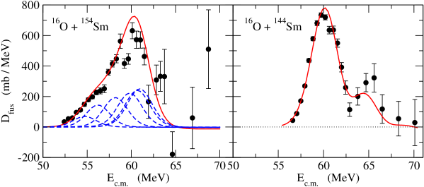
Figure 8: (The left panel) The fusion barrier distribution $D_{\rm fus}(E)=d^{2}(E\sigma_{\rm fus})/dE^{2}$ for the ¹⁶O+¹⁵⁴Sm reaction[18]. The solid line is obtained with the orientation average formula, which corresponds to the solid line in Fig. 5. The dashed lines indicate the contributions from six individual eigenbarriers (i.e., orientation angles). (The right panel) The fusion barrier distribution for the ¹⁶O+¹⁴⁴Sm reaction[18]. The solid line shows the result of the coupled-channels calculations which take into account the anharmonic double phonon excitations of ¹⁴⁴Sm [72, 73].

In the presence of channel couplings, Eq. (93) immediately leads to

$$D_{\rm fus}=\frac{d^{2}}{dE^{2}}[E\sigma_{\rm fus}(E)]=\sum_{\alpha}w_{\alpha}\,\frac{d^{2}}{dE^{2}}[E\sigma_{\rm fus}^{(\alpha)}(E)].$$ (99)

This function has been referred to as fusion barrier distribution. As an example, the left panel of Fig. 8 shows the barrier distribution for the ¹⁶O+¹⁵⁴Sm reaction, whose fusion cross sections have been already shown in Fig. 5. We replace the integral in Eq. (20) with the $(I_{\rm max}+2)$-point Gauss quadrature with $I_{\rm max}$=10. This corresponds to taking 6 different orientation angles[21]. The contributions from each eigenbarrier are shown by the dashed line in Fig. 8. The solid line is the sum of all the contributions, which is compared with the experimental data [18]. One can see that the calculation well reproduces the experimental data. Moreover, this analysis suggests that ¹⁵⁴Sm is a prolately deformed nucleus, since if it were an oblate nucleus, then lower potential barriers would have larger weights, and $D_{\rm fus}$ would be larger for smaller $E$, in contradiction to the experimentally observed barrier distribution[13].

The fusion barrier distribution has been extracted for many systems, see Ref. DHRS98 and references therein. The extracted barrier distributions were shown to be sensitive to the effects of channel-couplings and have provided a much more apparent way of understanding their effects on the fusion process than the fusion excitation functions themselves. These experimental data have thus enabled a detailed study of the effects of nuclear intrinsic excitations on fusion reactions, and have generated a renewed interest in heavy-ion subbarrier fusion reactions. An important point is that the nature of sub-barrier fusion reactions as a tunneling process exponentially amplifies the effects of detailed nuclear structure. Fusion barrier distribution makes this effect even more visible by plotting in the linear scale. The sub-barrier fusion reactions thus offer a novel way of nuclear spectroscopy which could be called a tunneling assisted nuclear spectroscopy. As an example, we mention that it was recently applied to elucidate the shape transition and the shape coexistence of Ge isotopes[91, 92]. It is worthwhile to mention also that the method of the barrier distribution has been successfully applied to heavy-ion quasi-elastic scattering [63, 93].

4.3 Eigenchannel representation

As we have discussed in the previous subsection, the barrier distribution representation, that is, the second derivative of $E\sigma_{\rm fus}$, has a clear physical meaning only if the excitation energy of the intrinsic motion is zero. The concept holds only approximately when the excitation energy is finite. Nonetheless, this analysis has been successfully applied to systems with relatively large excitation energies[18, 94, 79]. For example, the second derivative of $E\sigma_{\rm fus}$ for ¹⁶O + ¹⁴⁴Sm fusion reaction has a clear double-peaked structure (see the right panel of Fig. 8) [18, 94]. The coupled-channels calculation also yields a similar double-peaked structure of the fusion barrier distribution, and this structure has been interpreted in terms of the anharmonic octupole phonon excitations in ¹⁴⁴Sm [72, 73], whose excitation energy is 1.8 MeV for the first 3^- state. Also the analysis of the fusion reaction between ⁵⁸Ni and ⁶⁰Ni, where the excitation energies of quadrupole phonon states are 1.45 and 1.33 MeV, respectively, shows that the barrier distribution representation depends strongly on the number of phonon states included in coupled-channels calculations[79]. These analyses suggest that the representation of fusion process in terms of the second derivative of $E\sigma_{\rm fus}$ is a powerful method to study the details of the effects of nuclear structure, irrespective of the excitation energy of the intrinsic motion.

When the excitation energy of the intrinsic motion is finite, the barrier distribution is defined in terms of the eigen-channels. To illustrate it, first notice that Eq. (36) can be expressed as

$$P(E)=(T^{\dagger}T)_{n_{i}n_{i}},$$ (100)

using the completeness of the channels $n$ (we have suppressed the index $J$). We then introduce the eigenfunctions of the Hermitian operator $T^{\dagger}T$ as,

$$(T^{\dagger}T)|\phi_{k}\rangle=\gamma_{k}|\phi_{k}\rangle.$$ (101)

Using this basis, the penetrability is given by

$$P(E)=\sum_{k}|\langle\phi_{k}|n_{i}\rangle|^{2}\cdot\gamma_{k}.$$ (102)

When the excitation energies $\epsilon_{n}$ are all zero, as we have discussed in Sec. 4.1, one can diagonalize the coupling matrix $V_{nn^{\prime}}(r)$ with the basis set which is independent of the radial coordinate $r$. In this case, the matrix $T$ is diagonal on this basis, and the weight factor $|\langle\phi_{k}|n_{i}\rangle|^{2}$ is independent of $E$. Eq. (102) is a generalization of this scheme, which is applicable also when the excitation energies are non-zero.

Figure 9: (The left panel) The $s$-wave penetrabilities for the ¹⁶O+¹⁴⁴Sm reaction. The dotted line is obtained with the coupled-channels calculations with a single octupole phonon excitation in ¹⁴⁴Sm at 1.81 MeV with $\beta_{3}=0.205$. The solid lines show the eigenvalues of the square of the transmission matrix, $T^{\dagger}T$, defined by Eq. (101). The dashed lines denote the penetrabilities of the eigen barriers constructed by diagonalizing the coupling matrix at each $r$. (The right panel) The weight factors $|\langle\phi_{k}|n_{i}\rangle|^{2}$ defined in Eq. (102) as a function of energy.

Figure 9 shows the two eigenvalues $\gamma_{k}$ and the corresponding weight factors $|\langle\phi_{k}|n_{i}\rangle|^{2}$ as a function of $E$ for a single-phonon coupling calculation for the $s$-wave ¹⁶O+¹⁴⁴Sm reaction. To this end, we have taken into account couplings to the single octupole phonon state in ¹⁴⁴Sm at 1.81 MeV with the deformation parameter of $\beta_{3}$ = 0.205. The total probability $P(E)$, and the penetrability of the two eigenbarriers, obtained by diagonalizing the coupling matrix $V_{nn^{\prime}}(r)$ at each $r$, are also shown in the left panel of the figure by the dotted and the dashed lines, respectively. One can see that the two eigenvalues $\gamma_{k}$ approximately correspond to the penetrability of the eigenbarriers, and thus the factors $|\langle\phi_{k}|n_{i}\rangle|^{2}$ can be interpreted as the weight factors for each eigenbarrier. This implies that the fusion cross sections are still given by Eq. (93) even when the excitation energy is finite, except that the eigenbarriers are now constructed by diagonalizing the coupling matrix at each $r$. The weight factors do not vary strongly as a function of energy, suggesting that the concept of the fusion barrier distribution still holds to a good approximation even when the excitation energy of the intrinsic motion is finite. We have reached the same conclusion already in Ref. HTB97 using a different method from the one in this subsection. In contrast to the method in Ref. HTB97, the method in this subsection is more general since the applicability is not restricted to a two-level problem.

4.4 Adiabatic potential renormalization

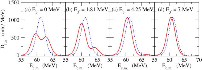
Figure 10: The fusion barrier distribution $D_{\rm fus}$ for the ¹⁶O+¹⁴⁴Sm reaction with several values of excitation energies, $E_{3^{-}}$, of the octupole vibration in ¹⁴⁴Sm. The solid lines are the results of the coupled-channels calculations which take into account the single octupole phonon excitation in ¹⁴⁴Sm, while the dashed lines are obtained without taking into account the channel coupling effect. The curvature $\hbar\Omega$ of the Coulomb barrier is 4.25 MeV in these calculations.

Given that the concept of fusion barrier distribution still holds even with a finite excitation energy, it is interesting to investigate how the fusion barrier distribution evolves as the excitation energy is varied. To this end, we carry out the coupled-channels calculations for the ¹⁶O+¹⁴⁴Sm reaction by taking into account the single octupole phonon excitation in ¹⁴⁴Sm. The solid line in Fig. 10 (a) shows the fusion barrier distribution $D_{\rm fus}$ when the excitation energy of the octupole vibration, $E_{3^{-}}$, is set to be zero. For comparison, the figure also shows the result of no-coupling calculation by the dashed line. In this case, the original single barrier splits into two eigenbarriers with equal weight, one corresponds to the effective channel $|0^{+}\rangle+|3^{-}\rangle$ and the other corresponds to $|0^{+}\rangle-|3^{-}\rangle$. The fusion barrier distribution is slightly asymmetric since the barrier positions, $R_{b}$, are different between the two effective channels (see Eq. (98)).

Figure 10(b) corresponds to the physical case of $E_{3^{-}}$ = 1.81 MeV. In this case, the barrier distribution still has a clear double peaked structure as in the experimental data[18, 94], but the lower energy barrier acquires more weight and the barrier distribution is highly asymmetric. The effective channels are now $\alpha|0^{+}\rangle+\beta|3^{-}\rangle$ (the lower energy barrier) and $\beta|0^{+}\rangle-\alpha|3^{-}\rangle$ (the higher energy barrier) with $\alpha>\beta>0$.

Figure 10(c) corresponds to the case where the excitation energy is set equal to the barrier curvature, $\hbar\Omega$, which is 4.25 MeV in the present calculations. In this case, the lower energy barrier has an appreciable weight although the weight factor for the higher energy barrier is not negligible. When the excitation energy is further increased, the weight for the lower energy barrier becomes close to unity as is shown in Fig. 10(d), and the fusion cross sections are approximately given by

$$\sigma_{\rm fus}(E)=\sigma_{\rm fus}(E;V(r)+\lambda_{0}(r)),$$ (103)

where $V(r)+\lambda_{0}(r)$ is the lowest eigen-barrier (see Eq. (93)). Therefore, the main effect of the coupling to a state with a large excitation energy is to simply introduce an energy-independent shift of the potential, $V(r)\to V(r)+\lambda_{0}(r)$. This phenomenon is called the adiabatic potential renormalization[96, 97, 98]. Typical examples in nuclear fusion include the couplings to the octupole vibration in ¹⁶O at 6.13 MeV [99] and to giant resonances in general.

In Refs. BT85 and THAB94, it has been argued based on the path integral approach to multi-dimensional tunneling that the transition from the sudden tunneling to the adiabatic tunneling takes place at the excitation energy around the barrier curvature, $\hbar\Omega$. That is, if the excitation energy is much larger than the barrier curvature, the channel coupling effect can be well expressed in terms of the adiabatic barrier renormalization. The numerical calculations shown in Fig. 10 are consistent with this criterion.

5 Fusion at deep subbarrier energies and dissipative tunneling

Although the coudpled-channels approach has been successful for heavy-ion reactions, many new challenges have been recognized in recent years. One of them is the surface diffuseness anomaly discussed in Sec. 2.1. Another challenge, which may also be related to the surface diffuseness anomaly[46], is an inhibition of fusion cross sections at deep subbarrier energies. This is a phenomenon found only recently, when fusion cross sections could become measured for several systems down to extremely low cross sections, up to the level of few nano barn (nb) [100, 101, 102, 103, 104]. These experimental data have shown that fusion cross sections systematically fall off much more steeply at deep-subbarrier energies with decreasing energy, compared to the expected energy dependence of cross sections around the Coulomb barrier. That is, the experimental fusion cross sections appear to be hindered at deep-subbarrier energies compared to the standard coupled-channels calculations that reproduce the experimental data at subbarrier energies, although the fusion cross sections are still enhanced with respect to a prediction of a single-channel potential model.

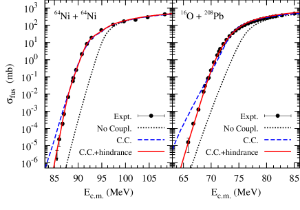
Figure 11: Fusion cross sections for the ⁶⁴Ni+⁶⁴Ni and ¹⁶O+²⁰⁸Pb systems as a function of the incident energy. The experimental data are taken from Refs. Jiang1 and Dasgupta07. The dotted and the dashed lines are the results of potential model and the standard coupled-channels calculations, respectively. The solid lines denote the result when the deep subbarrier fusion hindrance is described in the adiabatic model [108].

Two different models have been proposed so far in order to account for the deep subbarrier fusion hindrance. In the first model, assuming the frozen densities in the overlapping region (i.e., the sudden approximation), Misicu and Esbensen have introduced a repulsive core to an internucleus potential, which is originated from the Pauli exclusion principle [105]. See also Ref. DP03 for a related publication. The resultant potential is much shallower than the standard potentials, and hinders the fusion probability for high partial waves. In the second model, on the other hand, Ichikawa, Hagino, and Iwamoto have proposed an adiabatic approach by assuming a neck formation between the colliding nuclei in the overlap region[107, 108]. In this model, the reaction is assumed to take place slowly so that the density distribution has enough time to adjust to the optimized distribution. In this adiabatic model, the fusion hindrance originates from the tunneling of a thick one-body potential due to the neck formation. This model has achieved a comparable good reproduction of the experimental data to the sudden model, as is shown in Fig. 11.

The mechanism for the deep-subbarrier fusion hindrance has not yet been fully understood, as the two different models, in which the origin for the deep sub-barrier hindrance is considerably different from each other, account for the experimental data equally well. However, there is a certain thing which can be concluded by analyzing the threshold behavior in deep subbarrier fusion [100, 101, 109, 110, 111], independent of the fusion models[110]. In Refs. Jiang1,Jiang2 and Jiang3, the deep-subbarrier fusion hindrance has been analyzed using the astrophysical $S$ factor. It has been claimed that deep-subbarrier fusion hindrance sets in at the energy at which the astrophysical $S$ factor reaches its maximum. The authors of Refs. Jiang1,Jiang2 and Jiang3 even parametrized the threshold energy as a function of charge and mass numbers of the projectile and the target nuclei. The relation between the threshold for deep-subbarrier hindrance and the maximum of the $S$ factor is not clear physically, and thus it is not trivial how to justify the identification of the threshold energy with the maximum of the astrophysical $S$ factor. Nevertheless, it has turned out that the threshold energy so obtained closely follows the values of phenomenological internucleus potentials at the touching configuration [110]. This strongly suggests that the dynamics which takes place after the colliding nuclei touch each other somehow makes the astrophysical $S$ factor decrease as the incident energy decreases, leading to the fusion hindrance phenomenon. Notice that the fusion potential is almost the same between the sudden model and the adiabatic model before the touching (see Fig. 1 in Ref. IHI07b).

One important aspect of fusion reactions at deep sub-barrier energies is that the inner turning point of the potential may be located far inside the touching point of the colliding nuclei (see Fig. 1). After the two nuclei touch each other, many non-collective excitations of the unified one-body system are activated. As is well known from the Caldeira-Leggett model, couplings to those excitations lead to energy dissipation, which inhibits the tunneling probability[10]. The energy dissipation may occur also before the touching as a consequence of particle transfer processes to highly excited states in the target nucleus [112]. The phenomenon of deep subbarrier fusion hindrance may therefore be a realization of dissipative quantum tunneling, which has been extensively studied in many fields of physics and chemistry. A characteristic feature in nuclear fusion, which is absent or may not be important in dissipative tunneling in other fields, is that the couplings to (internal) environmental degrees of freedom gradually set in[121]. That is, before the touching the fully quantum mechanical coupled-channels approach with couplings to a few collective states of separate nuclei is adequate, which however gradually loses its validity after the touching point due to the dissipative couplings[104]. This is the region in which the conventional coupled-channels approach does not treat explicitly by introducing an absorbing potential or by imposing the incoming wave boundary condition. Although it is highly important to construct a model for nuclear fusion by taking into account the dissipative couplings [108, 113, 114] in order to clarify the deep subbarrier fusion hindrance, it is still a challenging open problem. To this end, a transition from the excitations of two separate nuclei in the entrance channel, which are included in the conventional coupled-channels calculations, to molecular excitations (i.e., the excitations of the combined mono-nuclear system) has to be described in a consistent and smooth manner [108, 115, 116, 117]. The development of quantum mechanical version of phenomenological classical models for deep inelastic collisions (DIC), such as the wall and window formulas for nuclear friction[118, 119, 120], will also be important in this respect.

6 Application of barrier distribution method to surface physics

The barrier distribution method discussed in Sec. 4 is applicable not only to heavy-ion subbarrier fusion reactions but also to any multi-channel tunneling problem. In general, the barrier distribution is defined as the first derivative of penetrability with respect to energy, $dP/dE$ (see Eq. (98)).

As an application of the barrier distribution method developed in nuclear physics to other fields, let us discuss a dissociative adsorption process of diatomic molecules on a metal surface. When molecular beams are injected on a certain metal, such as Cu and Pd, diatomic molecules are broken up in the vicinity of metal surface to two atoms due to the molecule-metal interactions before they stick to the metal. This process is referred to as dissociative adsorption, and has been extensively studied in surface science together with the inverse process, that is, associative desorption [122]. The adsorption process takes place by quantum tunneling at low incident energies, as there is a potential barrier between the two phases of the molecules, i.e., the molecular phase and the breakup phase with two separate atoms [122, 123]. The vibrational and rotational excitations of diatomic molecules play an important role in dissociative adsorption [124, 125, 126], as in heavy-ion subbarrier fusion reactions. The coupled-channels method has been utilized to discuss the effects of the internal excitations of molecules on dissociative adsorption[127, 128, 129, 130, 131, 132, 133, 134].

In this section, we discuss only the simplest case, that is, the effect of the rotational excitation on dissociative adsorption, while the vibrational degrees of freedom is assumed to be frozen in the ground state. In contrast to heavy-ion fusion reactions, the initial rotational state in the problem of dissociative adsorption is not necessarily the ground state. The initial rotational state of diatomic molecules can be in fact selected in molecular beams, and the experimental data of Michelsen et al. [125, 126] have indicated that the adsorption probability of D₂ molecules on Cu surface shows a nonmonotonic behavior as a function of the initial rotational state. That is, at a given incident energy, starting from the initial rotational state $L_{i}=0$, the adsorption probability first decreases for $L_{i}=5$ and then increases for $L_{i}=10$ and $L_{i}=14$ (see Fig. 9 in Ref. MRAZ93).

In order to explain this behavior, Diño, Kasai, and Okiji have considered a simple Hamiltonian for H₂ and D₂ molecules given by [130, 132]

$$H(s,\theta)=-\frac{\hbar^{2}}{2M}\frac{\partial^{2}}{\partial s^{2}}+\frac{\hbar^{2}}{2I(s)}\hat{\mbox{\boldmath$L$}}^{2}+V(s,\theta),$$ (104)

where $s$ is the one-dimensional reaction path in the two-dimensional potential energy surface spanned by the molecule-surface distance, $Z$, and the interatomic distance, $r$. The reaction takes place from $s=-\infty$, that corresponds to the approaching phase of molecules, to $s=+\infty$, where the incident molecule has broken up to two atoms. The sticking probability to the metal surface is identified as the penetrability of the potential barrier, $V$. $M$ in Eq. (104) is the mass for the translational motion of the diatomic molecule given by $M=2m$, where $m$ is the mass of the atom (i.e., $m=m_{H}$ for H₂ molecule and $m=m_{D}$ for D₂ molecule). $\theta$ is the molecular orientation angle, where $\theta$=0 corresponds to the configuration of the molecule perpendicular to the surface while $\theta=\pi/2$ to the configuration parallel to the surface. $\hat{\mbox{\boldmath$L$}}$ is the associated angular momentum operator. $I(s)$ is the momentum inertia for the rotational motion given by

$$I(s)=\mu r_{0}^{2}(1+fe^{\alpha s}),$$ (105)

where $\mu=m/2$ and $f$ is a parameter characterizing the $s$ dependence of the interatomic distance $r$, $r_{0}$ being the interatomic distance for an isolate molecule. The same parameter $\alpha$ as in Eq. (105) appears also in the potential energy, $V(s,\theta)$, which is parametrised as

$$V(s,\theta) = \frac{E_{a}}{\cosh^{2}(\alpha s)}(1-\beta\cos\theta^{2})+V_{1}\cos^{2}\theta\cdot\frac{1}{2}(1+\tanh(\alpha s)),$$ (106)

$$\equiv V_{0}(s)+V_{2}(s)Y_{20}(\theta),$$ (107)

with

$$V_{0}(s) = \frac{E_{a}}{\cosh^{2}(\alpha s)}\left(1-\frac{\beta}{3}\right)+\frac{V_{1}}{6}(1+\tanh(\alpha s)),$$ (108)

$$V_{2}(s) = -\frac{E_{a}}{\cosh^{2}(\alpha s)}\cdot\frac{2\beta}{3}\sqrt{\frac{4\pi}{5}}+\frac{1}{3}\sqrt{\frac{4\pi}{5}}V_{1}(1+\tanh(\alpha s)).$$ (109)

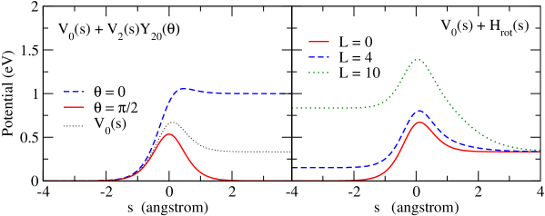
Figure 12: The potential energy for the dissociative adsorption process of H₂ molecule on metal surface given by Eq. (107). The parameters are $E_{a}$=0.536 eV, $V_{1}$=1.0 eV, $\alpha$=1.5 Å^-1, $\beta=0.25$, $r_{0}$=0.739 Å, and $f=0.14$. The left panel shows the potential for $L=0$ as a function of the reaction path coordinate $s$ for $\theta=0$ (the dashed line) and $\theta=\pi/2$ (the solid line), where $\theta$ is the molecular orientation angle ($\theta$=0 and $\theta=\pi/2$ correspond to the configurations with perpendicular and parallel to the metal surface, respectively) and $\hat{\mbox{\boldmath$L$}}$ is the associated angular momentum operator. The spherical part of the potential, $V_{0}(s)$, is also shown by the dotted line. The right panel shows the sum of spherical part of the potential, $V_{0}(s)$, and the rotational energy, $H_{\rm rot}(s)=L(L+1)\hbar^{2}/2I(s)$, for three different values of $L$.

The coupled-channels equations for the Hamiltonian (104) can be derived in the same manner as in Sec. 3. For scattering with the initial rotational angular momentum of molecules of $L_{i}$ and its $z$-component $M_{i}$, we expand the total wave function as

$$\Psi_{L_{i}M_{i}}(s,\theta)=\sum_{L}\phi_{LL_{i}}(s)Y_{LM_{i}}(\theta).$$ (110)

Notice that the Hamiltonian (104) conserve the value of $M_{i}$, as the coupling potential is proportional to $Y_{20}(\theta)$. The coupled-channels equations then read,

$$\left[-\frac{\hbar^{2}}{2M}\frac{d^{2}}{ds^{2}}+\frac{L(L+1)\hbar^{2}}{2I(s)}+V_{0}(s)-E\right]\phi_{LL_{i}}(s)+V_{2}(s)\sum_{L^{\prime}}\langle Y_{LM_{i}}|Y_{20}|Y_{L^{\prime}M_{i}}\rangle\phi_{L^{\prime}L_{i}}(s),$$ (111)

where the matrix element $\langle Y_{LM_{i}}|Y_{20}|Y_{L^{\prime}M_{i}}\rangle$ is given by

$$\langle Y_{LM_{i}}|Y_{20}|Y_{L^{\prime}M_{i}}\rangle=(-)^{M_{i}}\sqrt{\frac{5}{4\pi}}\sqrt{(2L+1)(2L^{\prime}+1)}\left(\begin{array}[]{ccc}L&2&L^{\prime}\\ 0&0&0\end{array}\right)\left(\begin{array}[]{ccc}L&2&L^{\prime}\\ -M_{i}&0&M_{i}\end{array}\right).$$ (112)

Noticing that $I(s)\to\mu r_{0}^{2}$ for $s\to-\infty$ and $I(s)\to 0$ for $s\to\infty$, these coupled-channels equations are solved by imposing the boundary conditions of

$$\phi_{LL_{i}}(s) = e^{ik_{L}s}\delta_{L,L_{i}}-\sqrt{\frac{k_{L_{i}}}{k_{L}}}\,R_{LL_{i}}e^{-ik_{L}s}~{}~{}~{}~{}~{}(s\to-\infty),$$ (113)

$$= \sqrt{\frac{k_{L_{i}}}{k}}\,T_{LL_{i}}e^{iks}~{}~{}~{}~{}~{}~{}~{}~{}~{}~{}~{}~{}~{}~{}~{}~{}~{}~{}~{}~{}~{}~{}~{}~{}~{}(s\to\infty),$$ (114)

where $k_{L}=\sqrt{2M(E-\epsilon_{L})/\hbar^{2}}$ with $\epsilon_{L}=L(L+1)\hbar^{2}/2\mu r_{0}^{2}$ and $k=\sqrt{2ME/\hbar^{2}}$. The adsorption probability for a given value of $L_{i}$ and $M_{i}$ is then obtained as

$$P_{L_{i}M_{i}}=\sum_{L}|T_{LL_{i}}|^{2}.$$ (115)

By making average over all possible $M_{i}$, the total adsorption probability for $L_{i}$ is given by

$$P_{L_{i}}=\frac{1}{2L_{i}+1}\sum_{M_{i}}P_{L_{i}M_{i}}.$$ (116)

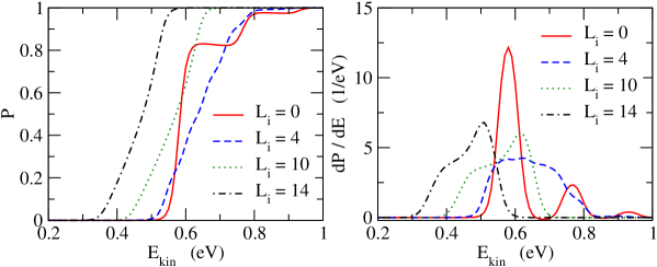
Figure 13: The results of the coupled-channels calculation for the dissociative adsorption process of H₂ molecules. The left panel shows the adsorption probability, $P$, while the right panels shows the barrier distribution defined as $dP/dE$ for several values of the initial angular momenta $L_{i}$ for the rotational state of the molecule as a function of the initial kinetic energy $E_{\rm kin}$.

Let us now solve the coupled-channels equations for H₂ molecules. The results are qualitatively the same also for D₂ molecules. Following Ref. DKO95, we take $E_{a}$=0.536 eV, $V_{1}$=1.0 eV, $\alpha$=1.5 Å^-1, $\beta=0.25$, and $r_{0}$=0.739 Å. For the factor $f$ in Eq. (105), we take $f=0.14$[135]. The potential with these parameters are shown in Fig. 12. The left panel shows the potential energy $V(s,\theta)$ given by Eq. (107) for two different values of $\theta$. For comparison, the figure also shows the spherical part of the potential, $V_{0}(s)$. One can see that the barrier is lower for the configuration parallel to the metal surface (that is, $\theta=\pi/2$) as compared to the configuration perpendicular to the surface, $\theta=0$. The right panel, on the other hand, shows the sum of the spherical part of the potential, $V_{0}(s)$, and the rotational energy, $H_{\rm rot}(s)=L(L+1)\hbar^{2}/2I(s)$, for three different values of $L$. Because of the $s$ dependence of the rotational moment of inertia, $I(s)$, the barrier height for the molecules incident from $s=-\infty$, that is, the difference between the energy at $s=0$ and that at $s=-\infty$ decreases as a function of $L$.

Figure 14: The results of the single-channel calculation, obtained by turning off all the coupling matrix elements in the coupled-channels equations except for the diagonal component. The left and the right panels show the adsorption probability, $P$, and the barrier distribution, $dP/dE$, respectively. The dotted lines denote the results when the initial rotational state is at $L_{i}=0$. The thin solid, the dot-dashed, and the thick solid lines are the results of $(L_{i},M_{i})=(2,0),(2,1)$, and (2,2), respectively. The dashed lines with the solid circles show the results for $L_{i}=2$ obtained by averaging all the $M_{i}$ components. For the barrier distributions shown in the right panel, the weight factors, 1/5 (for $M_{i}=0$) and 2/5 (for $M_{i}=1$ and 2), are multiplied.

The results of the coupled-channels calculations are shown in Fig. 13 for several values of initial rotational state, $L_{i}$, in which the adsorption probability is plotted as a function of the incident kinetic energy of the molecule, defined as $E=E_{\rm kin}+L_{i}(L_{i}+1)\hbar^{2}/2r_{0}^{2}$. As has been noted in Refs. DKO95 and DKO00, these calculations well account for the non-monotonic behavior of the adsorption probability as a function of $L_{i}$. The right panel shows the corresponding barrier distribution, $dP/dE$, obtained with the point difference formula with the energy step of 0.03 eV. One can clearly see different structures for each $L_{i}$. For $L_{i}=0$, the barrier distribution has three prominent peaks. These peaks are smeared for $L_{i}=4$, and at the same time, the center of mass of the distribution is shifted towards high energy, leading to the decrease of adsorption probability. This is due to the fact that the result for $L_{i}=4$ is actually given by the average over contributions from 9 different $M_{i}$ values. In order to demonstrate this effect, Fig. 14 shows the results of the single-channel calculations for $L_{i}=2$ with three different values of $M_{i}$ and its average. For comparison, the figure also shows the single-channel calculation for $L_{i}=0$ (the dotted line). We define the single-channel calculation as the one which neglects all the coupling terms in the coupled-channels equations (111) except for the diagonal term, $L=L^{\prime}$. Because of the properties of the spherical harmonics, the diagonal term of the coupling potential is attractive for $M_{i}=2$, while it is repulsive for $M_{i}=0$ and 1 (see Eq. (112)). The single peak in the barrier distribution for $L_{i}=0$ is then distributed to three peaks in the case of $L_{i}=4$, shifting the center of mass of the distribution slightly towards higher energy (notice that $-M_{i}$ gives the same contribution as $M_{i}$). With the off-diagonal components of the coupling potential, the distribution will be further smeared, as in the distribution for $L_{i}=4$ shown in Fig. 13. When the initial angular momentum is further increased, the barrier distribution starts moving towards lower energies, as seen in the figure for $L_{i}=10$ and 14, which enhances the adsorption probability as its consequence. This is mainly due to the fact that the barrier is lowered for a large value of rotational state, $L_{i}$, as has been shown in Fig. 12.

The barrier distribution representation of the tunneling probability provides a useful means to understand the underlying dynamics of dissociative adsorption process, as the shape of the distribution strongly reflects the molecular intrinsic motions. This would be even so, particularly when the rotational and the vibrational degrees are taken into account simultaneously[131, 133]. It will be an interesting future study to investigate how the barrier distribution behaves in the presence of the rotational excitation together with the vibrational excitation.

7 Summary and outlook

Recent developments in experimental techniques have enabled high precision measurements of heavy-ion fusion cross sections. Such high precision experimental data have elucidated the mechanism of subbarrier fusion reactions in terms of quantum tunneling of systems with many degrees of freedom. In particular, the effects of the coupling of the relative motion between the target and projectile nuclei to their intrinsic excitations have been transparently clarified through the barrier distribution representation of fusion cross sections.

The channel coupling effects can be taken into account most naturally with the coupled-channels method. When the excitation energy of an intrinsic motion to which the relative motion couples is zero, the concept of barrier distribution holds exactly. In this case, quantum tunneling takes place much faster than the intrinsic motion. The effects of the couplings can then be expressed in terms of the distribution of potential barriers, and the fusion cross sections are given as a weighted sum of fusion cross sections for the distributed barriers. The underlying structure of the barrier distribution can be most clearly investigated when the first derivative of barrier penetrability, $dP/dE$, is plotted as a function of energy. In heavy-ion fusion reactions, this quantity corresponds to the second derivative of $E\sigma_{\rm fus}$, which is referred to as fusion barrier distribution, $D_{\rm fus}$. The fusion barrier distribution has been extracted for many systems through the high precision experimental data of fusion cross sections, $\sigma_{\rm fus}$.

Even when the excitation energy of the intrinsic motion is not zero, the concept of fusion barrier distribution can be approximately generalized, using the eigen-channel representation of nuclear $S$-matrix, defined as the eigen-states of $S^{\dagger}S$. We have demonstrated that the barrier distribution shows a transition from the sudden to the adiabatic tunneling limits in a natural way as the excitation energy increases, where the potential is simply renormalized in the latter limit without affecting the shape of barrier distribution (i.e., the adiabatic barrier renormalization).

The barrier distribution representation is applicable also to other multi-channel quantum tunneling problems. A good example is the dissociative adsorption phenomenon in surface science. The rotational and vibrational excitations of diatomic molecules play an important role in the adsorption process. These effects can be described by the coupled-channels approach, and the barrier distribution can be defined as in heavy-ion subbarrier fusion reactions. The results of coupled-channels calculations have indicated that the barrier distribution representation provides a useful means in clarifying the underlying mechanism in the dynamics of surface interaction of molecules.

Although our understanding of subbarrier fusion reactions has considerably increased in the past decades, there are still many open problems in heavy-ion subbarrier fusion reactions. For example, it has not yet been understood completely how the hindrance of fusion cross sections with respect to the standard coupled-channels calculation takes place at deep subbarrier energies. A promising mechanism of the hindrance is that many non-collective channels are activated after the target and the projectile nuclei overlap with each other, and the relative energy is irreversibly dissipated to the intrinsic motions. This would occur only at deep subbarrier energies, in which the inner turning point of the potential barrier is located inside the touching radius of the two nuclei. This phenomenon may thus be a good example of dissipative quantum tunneling, which has been extensively discussed in many fields of physics and chemistry. A unique feature in nuclear physics is that the dissipative nature of the couplings gradually sets in, in a sense that the coupling is reversible before the touching and it gradually reveals the irreversible character as the overlap of the colliding nuclei increases. In order to gain a deep insight of this problem, it might be helpful to revisit heavy-ion deep inelastic collisions (DIC) from a more quantum mechanical point of view. This is important also in connection with the synthesis of superheavy elements by heavy ion collisions with large mass numbers, for which fusion cross is strongly hindered at energies near the bare Coulomb barrier.

Other important issues not covered in this paper include fusion of halo nuclei and the role of multi-nucleon transfer. For the former, there have been many debates concerning how the breakup process affects subbarrier fusion [136, 137, 138, 139, 140, 141, 142]. However the interplay between fusion and breakup involve many complex processes [24] and the role of breakup in fusion has not yet been understood completely. Moreover, particle transfer processes also affect both fusion and breakup in a non-trivial way, as has been found recently in ^6,7Li + ²⁰⁸Pb reactions[143] (see Ref. DHB99 for a review on subbarrier fusion of weakly bound stable nuclei, ^6,7Li and ⁹Be). A theoretical calculation has to take into account the fusion, transfer, and breakup processes simultaneously in a consistent manner. It remains a challenging problem to carry out such calculations, although the time-dependent wave packet approach [141] has been performed with a limited partition for the transfer channels. From experimental side, fusion cross sections for many neutron-rich nuclei do not appear to show any particular enhancement or hindrance [145, 146, 147, 148], but recent experimental data for ^12,13,14,15C+²³²Th reactions have shown that the fusion cross sections are enhanced for the ¹⁵C projectile as compared to those with the other C isotopes [149]. Again, several sort of transfer channels would have to be considered to understand the differences in the behavior of fusion cross sections [143, 150, 151, 152]. In particular, the multi-nucleon transfer process may play an important role in fusion of neutron-rich nuclei. Although there have been a few attempts to treat the multi-neutron transfer process in subbarrier fusion reactions [153, 154, 155, 156, 157], it has still been a challenging problem to include in a full quantum mechanical manner the multi-nucleon transfer processes consistently with inelastic channels by taking into account also the final $Q$-value distribution of transfer.

A much more challenging problem is to describe heavy-ion fusion reactions, thus many-particle tunneling[158], from fully quantum many-body perspectives, starting from nucleon degrees of freedom. The time-dependent Hartree-Fock (TDHF) theory has been widely employed to microscopically describe nuclear dynamics [159, 160]. It has been well known, however, that the TDHF method has a serious drawback that it cannot describe a many-particle tunneling phenomenon. In order to cure this problem, Bonasera and Kondratyev have introduced the imaginary time propagation [161, 162]. In this connection, we wish to mention that an alternative imaginary time approach, called the mean field tunneling theory, for quantum tunneling of systems with many degrees of freedom has been developed in Ref. KTAB03. The mean field tunneling theory is a reformulation of the dynamical norm method for quantum tunneling [164, 86], which evaluates the non-adiabatic effect on the tunneling rate through the change of the norm of the wave function for the intrinsic space during the evolution along the imaginary time axis. The mean field tunneling theory has been applied to quantum mechanically discuss electron screening effects in low energy nuclear reactions[163], while the dynamical norm method has been used to discuss the effects of nuclear oscillation on fission [164]. It would be an interesting challenge to develop a fully microscopic version of these methods and apply them to heavy-ion fusion reactions. More recently, Umar et al. have used the density constrained TDHF (DC-TDHF) method to analyze heavy-ion fusion reactions[165, 166, 167]. Even though these microscopic approaches seem promising, these are based on certain assumptions, such as a local collective potential with single-channel. It is thus not yet clear whether they are applicable to many-particle tunneling problems in general, such as two-proton radioactivity [168, 169, 170, 171, 172, 173] and alpha decays[174, 175, 176, 177, 178]. It would be an ultimate goal to develop a general microscopic theory which can describe several tunneling phenomena simultaneously, not only in nuclear physics but also in other fields of physics and chemistry. Such theory would naturally provide a way to describe the role of irreversibility (that is, the energy and angular momentum dissipations) as well as the density evolution after the touching in subbarrier fusion reactions without any assumption for the adiabaticity of the fusion process.

Appendix A Relation between surface diffuseness and barrier parameters

In this Appendix, we discuss the relation between the surface diffuseness parameter $a$ in a nuclear potential and the parameters which characterise the Coulomb barrer, that is, the curvature, the barrier height, and the barrier position. With such relation, one can estimate the value of $a$ from empirical barrier parameters.

For a given nuclear potential $V_{N}(r)$, the barrier position $R_{b}$ is obtained from the condition that the first derivative of the total potential is zero at $r=R_{b}$,

$$\left.\frac{d}{dr}V(r)\right|_{r=R_{b}}=\left[\frac{dV_{N}(r)}{dr}-\frac{Z_{P}Z_{T}e^{2}}{r^{2}}\right]_{r=R_{b}}=0.$$ (117)

The barrier height $V_{b}$ and the curvature $\Omega$ are then evaluated as

$$V_{b} = V_{N}(R_{b})+\frac{Z_{P}Z_{T}e^{2}}{R_{b}},$$ (118)

$$\Omega = \sqrt{-\frac{V_{N}^{{}^{\prime\prime}}(R_{b})+2Z_{P}Z_{T}e^{2}/R_{b}^{3}}{\mu}},$$ (119)

where $V_{N}^{{}^{\prime\prime}}(r)$ is the second derivative of the nuclear potential with respect to $r$.

A.1 Exponential potential

We first consider an exponential potential given by

$$V_{N}(r)=V_{0}e^{-r/a}.$$ (120)

From Eq. (117), the depth of the nuclear potential, $V_{0}$, is related to the charge product $Z_{P}Z_{T}$ as

$$-\frac{V_{0}}{a}e^{-R_{b}/a}-\frac{Z_{P}Z_{T}e^{2}}{R_{b}^{2}}=0.$$ (121)

From this equation, the barrier height and the curvature read

$$V_{b} = \frac{Z_{P}Z_{T}e^{2}}{R_{b}}\left(1-\frac{a}{R_{b}}\right),$$ (122)

$$\Omega^{2} = \frac{Z_{P}Z_{T}e^{2}}{\mu R_{b}^{2}}\left(\frac{1}{a}-\frac{2}{R_{b}}\right),$$ (123)

respectively.

A.2 Woods-Saxon potential

We next consider a Woods-Saxon potential given by

$$V_{N}(r)=-\frac{V_{0}}{1+e^{(r-R_{0})/a}}.$$ (124)

Combining Eqs. (117),(118), and (119), one finds that the surface diffuseness parameter $a$ is expressed in terms of $R_{b},V_{b}$ and $\Omega$ as

$$a=\frac{R_{b}}{-\frac{\mu\Omega^{2}R_{b}^{3}}{Z_{P}Z_{T}e^{2}}-2+\frac{2Z_{P}Z_{T}e^{2}}{Z_{P}Z_{T}e^{2}-R_{b}V_{b}}}.$$ (125)

Once the surface diffuseness parameter is thus evaluated, the other two parameters in the nuclear potential can be obtained as

$$1+e^{-x} = \frac{1}{a}\frac{R_{b}^{2}}{Z_{P}Z_{T}e^{2}}\left(\frac{Z_{P}Z_{T}e^{2}}{R_{b}}-V_{b}\right),$$ (126)

$$V_{0} = ae^{-x}(1+e^{x})^{2}\frac{Z_{P}Z_{T}e^{2}}{R_{b}^{2}},$$ (127)

where $x$ is defined as $(R_{b}-R_{0})/a$.

Appendix B Parabolic approximation and the Wong formula

If the Coulomb barrier is approximated by a parabola,

$$V(r)\sim V_{b}-\frac{1}{2}\mu\Omega^{2}(r-R_{b})^{2},$$ (128)

the corresponding penetrability can be evaluated analytically as

$$P(E)=\frac{1}{1+\exp\left[\frac{2\pi}{\hbar\Omega}(V_{b}-E)\right]}.$$ (129)

Using the parabolic approximation, Wong has derived an analytic expression for fusion cross sections [49]. He assumed that (i) the curvature of the Coulomb barrier, $\hbar\Omega$, is independent of the angular momentum $l$, and (ii) the position of the Coulomb barrier, $R_{b}$, is also independent of $l$, and the dependence of the penetrability on the angular momentum can be well approximated by shifting the incident energy as

$$P_{l}(E)=P_{l=0}\left(E-\frac{l(l+1)\hbar^{2}}{2\mu R_{b}^{2}}\right).$$ (130)

If many partial waves contribute to fusion cross section, the sum in Eq. (17) may be replaced by an integral,

$$\sigma_{\rm fus}(E)=\frac{\pi}{k^{2}}\int_{0}^{\infty}dl~{}(2l+1)P_{l}(E).$$ (131)

Changing the variable from $l$ to $l(l+1)$, the integral can be explicitly carried out, leading to the Wong formula [49]

$$\sigma_{\rm fus}(E)=\frac{\hbar\Omega}{2E}R_{b}^{2}\ln\left[1+\exp\left(\frac{2\pi}{\hbar\Omega}(E-V_{b})\right)\right].$$ (132)

At energies well above the Coulomb barrier, this formula reduces to the classical expression of fusion cross section given by Eq. (94).

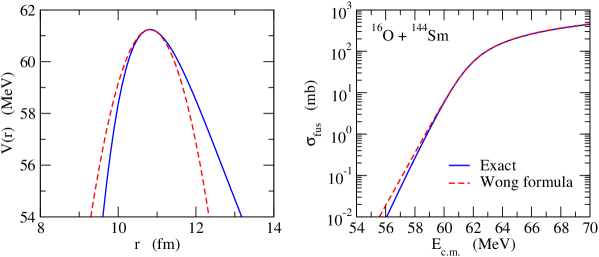
Figure 15: (The left panel) The Coulomb barrier for the ¹⁶O+¹⁴⁴Sm system shown in Fig. 1 (the solid line) and its parabolic approximation (the dashed line). (The right panel) Comparison of the corresponding fusion cross sections obtained by numerically solving the Schrödinger equation without resorting to the parabolic approximation (the solid line) and those obtained with the Wong formula, Eq. (132).

The left panel of Fig. 15 shows the parabolic approximation to the Coulomb barrier for the ¹⁶O + ¹⁴⁴Sm system shown in Fig. 1. Because of the long ranged Coulomb interaction, the Coulomb barrier is asymmetric and the parabolic potential has a smaller width compared with the realistic potential. Nevertheless, the Wong formula for fusion cross sections, Eq. (132), works well except at energies well below the barrier, where the parabolic approximation breaks down (see the right panel of Fig. 15).

Even though the Wong formula appears to work well for the single-channel potential model, one can still discuss the corrections to it. The first correction is with respect to the integral in Eq. (131). To discuss the correction, we first notice that replacing the sum in Eq. (17) with the integral in Eq. (131) is equivalent to taking only the leading term ($m=0$) of the exact Poisson sum formula,

$$\sigma_{\rm fus}(E)=\frac{\pi}{k^{2}}\sum_{l}(2l+1)P_{l}(E)=\frac{2\pi}{k^{2}}\sum_{m=-\infty}^{\infty}\int^{\infty}_{0}\lambda P(E;\lambda)e^{2\pi mi\lambda}d\lambda,$$ (133)

where $P(E;\lambda)$ is any smooth function of $\lambda$ satisfying $P(E,l+1/2)=P_{l}(E)$ [81]. Poffe, Rowley, and Lindsay have evaluated the contribution of the next most important terms, $m=\pm 1$[179]. These terms lead to an oscillatory contribution to the fusion cross sections,

$$\sigma_{\rm fus}(E)=\sigma_{W}(E)+\sigma_{\rm osc}(E),$$ (134)

where $\sigma_{W}(E)$ is given by Eq. (132), while the oscillatory part $\sigma_{\rm osc}(E)$ is given by

$$\sigma_{\rm osc}(E)=4\pi\mu R_{b}^{2}\frac{\hbar\Omega}{k^{2}}\exp\left(-\frac{\pi\mu R_{b}^{2}\hbar\Omega}{l_{g}+\frac{1}{2}}\right)\sin(2\pi l_{g}).$$ (135)

Here, $l_{g}$ is the grazing angular momentum satisfying

$$E=V(r)+\frac{l_{g}(l_{g}+1)\hbar^{2}}{2\mu R_{b}^{2}}.$$ (136)

For heavy systems, the oscillatory part of fusion cross sections, $\sigma_{\rm osc}$, is usually much smaller than the leading term, $\sigma_{W}$. However, for light symmetric systems such as ¹²C+¹²C, the oscillatory part becomes significant[179, 180, 181, 182, 183]. For a system of identical spin-zero bosons, the factor $(1+(-1)^{l})$ has to be multiplied in the sum in Eq. (17) due to the symmetrization effect, making the contributions of all the odd partial waves vanish. In this case, the leading term of the fusion cross section is still given by the Wong formula, Eq. (132), while the oscillatory part becomes [179]

$$\sigma_{\rm osc}(E)=4\pi\mu R_{b}^{2}\frac{\hbar\Omega}{k^{2}}\exp\left(-\frac{\pi\mu R_{b}^{2}\hbar\Omega}{2l_{g}+1}\right)\sin(\pi l_{g}).$$ (137)

Fig. 16 shows the fusion cross sections for the ¹²C+¹²C reaction obtained with a parabolic potential with $V_{b}=5.6$ MeV, $R_{b}$=6.3 fm, and $\hbar\Omega=3$ MeV. The solid line shows the result of the exact summation of partial wave contributions with Eq. (130), while the dashed line shows a sum of Eqs. (132) and (137). A separate contribution from the Wong formula, Eq. (132), is also shown by the dotted line. It is seen that the oscillation of fusion cross sections can be well reproduced with the formula given by Eq. (137).

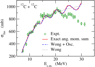
Figure 16: The fusion excitation function for the ¹²C+¹²C system. The solid line is obtained by carrying out exactly the angular momentum sum (with the symmetrization factor) in Eq. (17) with a parabolic potential with $V_{b}=5.6$ MeV, $R_{b}$=6.3 fm, and $\hbar\Omega=3$ MeV. The barrier position and the curvature are assumed to be independent of the angular momentum $l$. The dotted line is obtained with the Wong formula, Eq. (132), while the dashed line is obtained as a sum of the Wong formula and the oscillatory cross sections given by Eq. (137). The experimental data are taken from Ref. S76.

The second correction to the Wong formula is the angular momentum dependence of the barrier radius[184]. Up to the first order of $\hbar^{2}/\mu^{2}\Omega^{2}R_{b}^{4}$, Balantekin et al. have shown that the barrier radius for the $l$-th partial wave $R_{bl}$ is given by

$$R_{bl}=R_{b}-\frac{l(l+1)\hbar^{2}}{\mu^{2}\Omega^{2}R_{b}^{3}}.$$ (138)

This equation indicates that the barrier position decreases as the angular momentum $l$ increases. At energies well above the barrier, the classical fusion cross sections are then modified to [184]

$$\sigma_{\rm fus}(E)=\pi R_{b}^{2}\left(1-\frac{V_{b}}{E}\right)-\frac{2\pi}{\mu\Omega^{2}E}(E-V_{b})^{2}~{}~{}~{}~{}~{}~{}(E\gg V_{b}).$$ (139)

Comparison between Eqs. (94) and (139) shows that the Wong formula slightly overestimates fusion cross sections at energies well above the Coulomb barrier.

Appendix C Multiphonon coupling

In this Appendix, we show that the dimension of coupled-channels equations can be reduced for vibrational couplings by introducing effective multi-phonon channels. Suppose that we have two modes of vibrational excitations (e.g., a quadrupole and an octupole modes), and consider the excitation operator

$$\hat{O}=\beta_{1}(a_{1}^{\dagger}+a_{1})+\beta_{2}(a_{2}^{\dagger}+a_{2}),$$ (140)

and the phonon Hamiltonian

$$H_{0}=\hbar\omega_{1}a_{1}^{\dagger}a_{1}+\hbar\omega_{2}a_{2}^{\dagger}a_{2},$$ (141)

where $a_{1}^{\dagger}$ and $a_{2}^{\dagger}$ are the phonon creation operator for the first and the second modes, respectively. $\beta_{i}~{}(i=1,2)$ are the coupling constants, while $\hbar\omega_{i}~{}(i=1,2)$ are the phonon excitation energy for each mode. We have shifted the phonon energies so that the ground state is at zero energy.

If we truncate the phonon space up to the one phonon states, we have three basis states, $|00\rangle,|10\rangle$, and $|01\rangle$, where the state $|n_{1}n_{2}\rangle$ corresponds to the product state of $n_{1}$ phonon state for the first mode and $n_{2}$ phonon state for the second mode. Here we have included the states with $n_{1}+n_{2}\leq 1$. The matrix elements of the operator $H_{0}+\hat{O}$ with these basis states read,

$$H_{0}+\hat{O}=\left(\begin{array}[]{ccc}0&\beta_{1}&\beta_{2}\\ \beta_{1}&\hbar\omega_{1}&0\\ \beta_{2}&0&\hbar\omega_{2}\\ \end{array}\right),$$ (142)

It is easy to see that the ground state $|00\rangle$ couples only to a particular combination of $|10\rangle$ and $|01\rangle$[69],

$$|\tilde{1}\rangle=\frac{1}{\sqrt{\beta_{1}^{2}+\beta_{2}^{2}}}\,(\beta_{1}|10\rangle+\beta_{2}|01\rangle),$$ (143)

with

$$\hat{O}|00\rangle=\sqrt{\beta_{1}^{2}+\beta_{2}^{2}}\,|\tilde{1}\rangle.$$ (144)

The other combination of $|10\rangle$ and $|01\rangle$, $\beta_{2}|10\rangle-\beta_{1}|01\rangle$, couples neither to $|00\rangle$ nor $|\tilde{1}\rangle$, and this can be removed from the coupled-channels calculation if the excitation energies of the two modes are the same, $\hbar\omega_{1}=\hbar\omega_{2}\equiv\hbar\omega$. In this case, the dimension of the coupled-channels equations can be reduced to two with a modified strength as[69],

$$H_{0}+\hat{O}=\left(\begin{array}[]{cc}0&\bar{\beta}\\ \bar{\beta}&\hbar\omega\end{array}\right),$$ (145)

where $\bar{\beta}$ is defined by $\bar{\beta}=\sqrt{\beta_{1}^{2}+\beta_{2}^{2}}$. One can easily generalize this scheme to higher members of phonon states. The resultant matrix is equivalent to that for a single phonon mode with the effective strength $\bar{\beta}$. For instance, when the phonon space is truncated at the two-phonon states, the coupling matrix reads

$$H_{0}+\hat{O}=\left(\begin{array}[]{ccc}0&\bar{\beta}&0\\ \bar{\beta}&\hbar\omega&\sqrt{2}\bar{\beta}\\ 0&\sqrt{2}\bar{\beta}&2\hbar\omega\end{array}\right),$$ (146)

where the effective two phonon state is defined as

$$|\tilde{2}\rangle=\frac{1}{\beta_{1}^{2}+\beta_{2}^{2}}\left(\beta_{1}^{2}|20\rangle+\sqrt{2}\beta_{1}\beta_{2}|11\rangle+\beta_{2}^{2}|02\rangle\right).$$ (147)

References

- [1] G. Gamow, Z.Phys. 51 (1928), 204.
- [2] R.W. Gurney and E.U. Condon, Nature 122 (1928), 439; Phys. Rev. 33 (1929), 127.
- [3] P.L. Kapur and R. Peierls, Proc. Roy. Soc. A163 (1937), 606.
- [4] T. Banks, C.M. Bender and T.T. Wu, Phys. Rev. D8 (1973), 3346; D8 (1973), 3366.
- [5] J.L. Gervais and B. Sakita, Phys. Rev. D16 (1977), 3507.
- [6] D.M. Brink, M.C. Nemes and D. Vautherin, Ann. Phys. (N.Y.) 147 (1983), 171.
- [7] A. Schmid, Ann. Phys. (N.Y.) 170 (1986), 333.
- [8] S. Takada and H. Nakamura, J. Chem. Phys. 100 (1994), 98.
- [9] D.B. Schwartz, B. Sen, C.N. Archie, and J.E. Lukens, Phys. Rev. Lett. 55 (1985), 1547.
- [10] A.O. Caldeira and A.J. Leggett, Phys. Rev. Lett. 46 (1981), 211; Ann. of Phys. (N.Y.) 149 (1983), 374.
- [11] Proceedings of the Fourth International Symposium on Foundations of Quantum Mechanics, edited by M. Tsukada et al., Japanese Journal of Applied Physics Series Vol. 9 ( Publication Office of Japanese Journal of Applied Physics, Tokyo, 1993).
- [12] A.B. Balantekin and N. Takigawa, Rev. Mod. Phys. 70 (1998), 77.
- [13] M. Dasgupta, D.J. Hinde, N. Rowley, and A.M. Stefanini, Annu. Rev. Nucl. Part. Sci. 48 (1998), 401.
- [14] M. Beckerman, Rep. Prog. Phys.51 (1988), 1047; Phys. Rep. 129 (1985), 145.
- [15] S.G. Steadman and M.J. Rhoades-Brown, Ann. Rev. Nucl. Part. Sci. 36 (1986), 649.
- [16] W. Reisdorf, J. of Phys. G20 (1994), 1297.
- [17] R.G. Stokstad, Y. Eisen, S. Kaplanis, D. Plete, U. Smilansky, and I. Tserruya, Phys. Rev. Lett. 41 (1978), 465; Phys. Rev. C21 (1980), 2427.
- [18] J.R. Leigh, M. Dasgupta, D.J. Hinde, J.C. Mein, C.R. Morton, R.C. Lemmon, J.P. Lestone, J.O. Newton, H. Timmers, J.X. Wei, and N. Rowley, Phys. Rev. C52 (1995), 3151.
- [19] C.H. Dasso, S. Landowne, and A. Winther, Nucl. Phys. A405 (1983), 381; ibid A407 (1983), 221.
- [20] H. Esbensen, Nucl. Phys. A352 (1981), 147.
- [21] M.A. Nagarajan, A.B. Balantekin, and N. Takigawa, Phys. Rev. C34 (1986), 894.
- [22] N. Rowley, G.R. Satchler, and P.H. Stelson, Phys. Lett. B254 (1991), 25.
- [23] J.X. Wei, J.R. Leigh, D.J. Hinde, J.O. Newton, R.C. Lemmon, S. Elfstrom, J.X. Chen, and N. Rowley, Phys. Rev. Lett. 67 (1991), 3368.
- [24] L.F. Canto, P.R.S. Gomes, R. Donangelo, and M.S. Hussein, Phys. Rep. 424 (2006), 1.
- [25] J.F. Liang and C. Signorini, Int. J. of Mod. Phys. E14 (2005), 1121.
- [26] P. Armbruster, Annu. Rev. Nucl. Part. Sci. 50 (2000), 411.
- [27] P. Armbruster and G. Münzenberg, Euro. Phys. J. H37 (2012), 237.
- [28] G.R. Satchler and W.G. Love, Phys. Rep. 55 (1979), 183.
- [29] M.E. Brandan and G.R. Satchler, Phys. Rep. 285 (1997), 143.
- [30] D.T. Khoa and G.R. Satchler, Nucl. Phys. A668 (2000), 3.
- [31] D.T. Khoa, G.R. Satchler, and W. von Oertzen, Phys. Rev. C56 (1997), 954.
- [32] D.T. Khoa, Phys. Rev. C63 (2001), 034007.
- [33] B. Sinha, Phys. Rep. 20 (1975), 1.
- [34] B. Sinha and S.A. Moszkowski, Phys. Lett. 81B (1979), 289.
- [35] R.A. Broglia and A. Winther, Heavy-Ion Reactions, (Addison-Wesley, New York, 1991).
- [36] Ö. Akyüz and A. Winther, in Nuclear Structure and Heavy-Ion Collisions, Proceedings of the International School of Physics “Enrico Fermi, ”Course LXXVII, Varenna, 1979, edited by R.A. Broglia et al. (North- Holland, Oxford, 1981).
- [37] K. Hagino, T. Takehi, A.B. Balantekin, and N. Takigawa, Phys. Rev. C71 (2005), 044612.
- [38] K. Washiyama, K. Hagino, and M. Dasgupta, Phys. Rev. C73 (2006), 034607.
- [39] L.R. Gasques et al., Phys. Rev. C76 (2007), 024612.
- [40] M. Evers et al., Phys. Rev. C78 (2008), 034614.
- [41] C.J. Lin et al., Phys. Rev. C79 (2009), 064603.
- [42] J.O. Newton, C.R. Morton, M. Dasgupta, J.R. Leigh, J.C. Mein, D.J. Hinde, H. Timmers, and K. Hagino, Phys. Rev. C64 (2001), 064608.
- [43] J.O. Newton, R.D. Butt, M. Dasgupta, D.J. Hinde, I.I. Gontchar, C.R. Morton, and K. Hagino, Phys. Lett. B586 (2004), 219; Phys. Rev. C70 (2004), 024605.
- [44] A. Mukherjee, D.J. Hinde, M. Dasgupta, K. Hagino, J.O. Newton, R.D. Butt, Phys. Rev. C75 (2007), 044608.
- [45] I.I. Gontchar, D.J. Hinde, M. Dasgupta, and J.O. Newton, Phys. Rev. C69 (2004), 024610.
- [46] K. Hagino, N. Rowley, and M. Dasgupta, Phys. Rev. C67 (2003), 054603.
- [47] S. Landowne and S.C. Pieper, Phys. Rev. C29 (1984), 1352.
- [48] K. Hagino, N. Rowley, and A.T. Kruppa, Comp. Phys. Comm. 123 (1999), 143.
- [49] C.Y. Wong, Phys. Rev. Lett. 31 (1973), 766.
- [50] Z.E. Switkowski, R.G. Stokstad, and R.M. Wieland, Nucl. Phys. A279 (1977), 502.
- [51] L.F. Canto, P.R.S. Gomes, J. Lubian, L.C. Chamon, and E. Crema, J. of Phys. G36, 015109 (2009); Nucl. Phys. A821, 51 (2009).
- [52] P.R.S. Gomes, J. Lubian, and L.F. Canto, Phys. Rev. C79, 027606 (2009).
- [53] A.B. Balantekin, S.E. Koonin, and J.W. Negele, Phys. Rev. C28 (1983), 1565.
- [54] M.W. Cole and R.H. Good, Phys. Rev. A18 (1978), 1085.
- [55] M. Inui and S.E. Koonin, Phys. Rev. C30, 175 (1984).
- [56] K. Hagino and Y. Watanabe, Phys. Rev. C76 (2007), 021601(R).
- [57] S. Yusa, K. Hagino, and N. Rowley, Phys. Rev. C82 (2010), 024606; C85 (2012), 054601.
- [58] A. Bohr and B. Mottelson, Nuclear Structure (Benjamin, New York, 1975), vol. 2.
- [59] G.F. Bertsch and R.A. Broglia, Oscillations in Finite Quantum Systems (Cambridge University Press, Cambridge, 1994).
- [60] M.N. Harakeh and A. van der Woude, Giant Resonances, (Oxford University Press, Oxford, 2001).
- [61] W. Scobel, A. Mignerey, M. Blann, and H.H. Gutbrod, Phys. Rev. C11 (1975), 1701.
- [62] T. Rumin, K. Hagino, and N. Takigawa, Phys. Rev. C63 (2001), 044603.
- [63] K. Hagino and N. Rowley, Phys. Rev. C69 (2004), 054610.
- [64] Y. Aritomo, K. Hagino, K. Nishio, and S. Chiba, Phys. Rev. C85 (2012), 044614.
- [65] A.R. Edmonds, Angular Momentum in Quantum Mechanics, (Princeton University Press, Princeton, New Jersey, 1960), Eq. (7.1.6).
- [66] N. Takigawa and K. Ikeda, in Proceedings of the Symposium on Many Facets of Heavy Ion Fusion Reactions, edited by W. Henning et al.(Argonne National Laboratory Report No. ANL-PHY-87-1), 1986, p.613.
- [67] O. Tanimura, Phys. Rev. C35 (1987), 1600; O. Tanimura, Z. Phys. A327, 413 (1987).
- [68] H. Esbensen, S. Landowne, and C. Price, Phys. Rev. C36 (1987), 1216; Phys. Rev. C36 (1987), 2359.
- [69] A.T. Kruppa, P. Romain, M.A. Nagarajan, and N. Rowley, Nucl. Phys. A560 (1993), 845.
- [70] J. Gomez-Camacho and R.C. Johnson, J. Phys. G12 (1986), L235; J. Phys. G14 (1988), 609.
- [71] K. Hagino, N. Takigawa, M. Dasgupta, D.J. Hinde, and J.R. Leigh, Phys. Rev. C55 (1997), 276.
- [72] K. Hagino, N. Takigawa, and S. Kuyucak, Phys. Rev. Lett. 79 (1997), 2943.
- [73] K. Hagino, S. Kuyucak, and N. Takigawa, Phys. Rev. C57 (1998), 1349.
- [74] J. de Boer and J. Eichler, Advances in Nuclear Physics, (Plenum, New York, 1968), vol. 1, p. 1.
- [75] C.H. Dasso, J. Fernández-Niello, and A. Vitturi, Phys. Rev. C55 (1997), 2112.
- [76] H. Esbensen and S. Landowne, Phys. Rev. C35 (1987), 2090.
- [77] A.B. Balantekin, J.R. Bennett, and S. Kuyucak, Phys. Rev. C 48 (1993), 1269; Phys. Rev. C49 (1994), 1079.
- [78] N. Rowley, in Proceedings of the International Workshop on Heavy-Ion Fusion: Exploring the Variety of Nuclear Properties, edited by A.M. Stefanini et al. (World Scientific, Singapore, 1994), p.66.
- [79] A.M. Stefanini et al., Phys. Rev. Lett. 74 (1995), 864.
- [80] M.W. Kermode and N. Rowley, Phys. Rev. C48 (1993), 2326.
- [81] D.M. Brink, Semi-Classical Methods for Nucleus-Nucleus Scattering, (University Press, Cambridge, 1985).
- [82] D.M. Brink and U. Smilansky, Nucl. Phys. A405 (1983), 301.
- [83] D.M. Brink and N. Takigawa, Nucl. Phys. A279 (1977), 159.
- [84] S.Y. Lee, N. Takigawa and C. Marty, Nucl. Phys. A308 (1978), 161.
- [85] S.Y. Lee and N. Takigawa, Nucl. Phys. A308 (1978), 189.
- [86] K. Hagino and A.B. Balantekin, Phys. Rev. A70 (2004), 032106.
- [87] M.A. Nagarajan, N. Rowley, and R. Lindsay, J. Phys. G12 (1986), 529.
- [88] M.V. Andres, N. Rowley, and M.A. Nagarajan, Phys. Lett. 202B (1988), 292.
- [89] N. Takigawa, Y. Alhassid, and A.B. Balantekin, Phys. Rev. C45 (1992), 1850.
- [90] K. Hagino, N. Takigawa, J.R. Bennett, and D.M. Brink, Phys. Rev. C51 (1995), 3190.
- [91] H. Esbensen, Phys. Rev. C68 (2003), 034604.
- [92] Muhammad Zamrun F.,Zakarya Mohamed Mohamed Mahmoud, N. Takigawa and K. Hagino, Phys. Rev. C81 (2010), 044609 (2010).
- [93] H. Timmers, M. Dasgupta, D.J. Hinde, J.R. Leigh, R.C. Lemmon, J.C. Mein, C.R. Morton, J.O. Newton, and N. Rowley, Nucl. Phys. A584 (1994), 190.
- [94] C.R. Morton, M. Dasgupta, D.J. Hinde, J.R. Leigh, R.C. Lemmon, J.P. Lestone, J.C. Mein, J.O. Newton, H. Timmers, N. Rowley, and A.T. Kruppa, Phys. Rev. Lett. 72, 4074(1994).
- [95] K. Hagino, N. Takigawa, and A.B. Balantekin, Phys. Rev. C 56 (1997), 2104.
- [96] O. Tanimura, J. Makowka, and U. Mosel, Phys. Lett. 163B (1985), 317.
- [97] A.B. Balantekin and N. Takigawa, Ann. Phys. (N.Y.) 160 (1985), 441.
- [98] N. Takigawa, K. Hagino, M. Abe, and A.B. Balantekin, Phys. Rev. C49 (1994), 2630.
- [99] K. Hagino, N. Takigawa, M. Dasgupta, D.J. Hinde, and J.R. Leigh, Phys. Rev. Lett. 79 (1997), 2014.
- [100] C.L. Jiang et al., Phys. Rev Lett.89 (2002), 052701; Phys. Rev Lett.93 (2004), 012701.
- [101] C.L. Jiang et al., Phys. Rev C71 (2005), 044613; Phys. Rev C78 (2008), 017601; Phys. Rev C81 (2010), 024611.
- [102] A.M. Stefanini et al., Phys. Rev. C78 (2008), 044607; G. Montagnoli et al., Phys. Rev. C82 (2010), 064609.
- [103] C.L. Jiang et al., Phys. Rev. C82 (2010), 041601(R); G. Montagnoli et al., Phys. Rev. C85 (2012), 024607.
- [104] M. Dasgupta et al., Phys. Rev. Lett. 99 (2007), 192701.
- [105] S. Misicu and H. Esbensen, Phys. Rev. Lett. 96 (2006), 112701; Phys. Rev. C75 (2007), 034606.
- [106] C.H. Dasso and G. Pollarolo, Phys. Rev. C68 (2003), 054604.
- [107] T. Ichikawa, K. Hagino, and A. Iwamoto, Phys. Rev. C75 (2007), 057603; Phys. Rev. Lett. 103 (2009), 202701.
- [108] T. Ichikawa, K. Hagino, and A. Iwamoto, Phys. Rev. Lett. 103 (2009), 202701.
- [109] C. L. Jiang, H. Esbensen, B. B. Back, R.V.F. Janssens, and K.E. Rehm, Phys. Rev. C69 (2004), 014604; C.L. Jiang, B.B. Back, H. Esbensen, R.V.F. Janssens, and K.E. Rehm, Phys. Rev. C73 (2006), 014613.
- [110] T. Ichikawa, K. Hagino, and A. Iwamoto, Phys. Rev. C 75 (2007), 064612.
- [111] Ei Shwe Zin Thein, N.W. Lwin, and K. Hagino, Phys. Rev. C85 (2012), 057602.
- [112] M. Evers et al., Phys. Rev. C84 (2011), 054614.
- [113] A. Diaz-Torres, D.J. Hinde, M. Dasgupta, G.J. Milburn, J.A. Tostevin, Phys. Rev. C78 (2008), 064604.
- [114] B.V. Carlson, O. Civitarese, M.S. Hussein, and A. Szanto de Toledo, Ann. of Phys. (N.Y.) 169 (1986), 167.
- [115] D. Hahn, G. Terlecki, and W. Scheid, Nucl. Phys. A325 (1979), 283.
- [116] S. Mukamel, U. Smilansky, D.H.E. Gross, K. Möhring, and M.I. Sobel, Nucl. Phys. A366 (1981), 339.
- [117] D.H.E. Gross, K. Möhring, S. Mukamel, U. Smilansky, and M.I. Sobel, Nucl. Phys. A378 (1982), 375.
- [118] J. Blocki, Y. Boneh, J.R. Nix, J. Randrup, M. Robel, A.J. Sierk, and W.J. Swiatecki, Ann. of Phys. (N.Y.) 113 (1978), 330.
- [119] J. Randrup, Ann. of Phys. (N.Y.) 171 (1986), 28.
- [120] T. Dossing and J. Randrup, Nucl. Phys. A475 (1987), 557.
- [121] We thank M. Dasgupta and D.J. Hinde for discussions on this point.
- [122] G.R. Darling and S. Holloway, Rep. Prog. Phys. 58 (1995), 1595, and referenes therein.
- [123] B. Hammer, M. Scheffler, K.W. Jacobsen, and J.K. Nørskov, Phys. Rev. Lett. 73 (1994), 1400.
- [124] C.T. Rettner, D.J. Auerbach, and H.A. Michelsen, Phys. Rev. Lett. 68 (1992), 1164.
- [125] H.A. Michelsen, C.T. Rettner, and D.J. Auerbach, Phys. Rev. Lett. 69 (1992), 2678.
- [126] H.A. Michelsen, C.T. Rettner, and D.J. Auerbach, and R.N. Zare, J. Chem. Phys. 98 (1993), 8294.
- [127] W. Brenig and H. Kasai, Surf. Sci. 213 (1989), 170.
- [128] H. Kasai and A. Okiji, Prog. in Surf. Sci. 44 (1993), 101.
- [129] Y. Chiba and W. Brenig, Surf. Sci. 306 (1994), 406.
- [130] W.A. Diño, H. Kasai, and A. Okiji, J. of Phys. Soc. Japan 64 (1995), 2478; Phys. Rev. Lett. 78 (1997), 286.
- [131] W.A. Diño, H. Kasai, and A. Okiji, Surf. Sci. 363 (1996), 52.
- [132] W.A. Diño, H. Kasai, and A. Okiji, Prog. in Surf. Sci. 63 (2000), 63.
- [133] Y. Miura, H. Kasai, and W.A. Diño, J. of Phys. Soc. Japan 68 (1999), 887.
- [134] A. Gross, S. Wilke, and M. Scheffler, Phys. Rev. Lett. 75 (1995), 2718.
- [135] W.A. Diño, private communications.
- [136] M.S. Hussein, M.P. Pato, L.F. Canto, and R. Donangelo, Phys. Rev. C46 (1992), 377.
- [137] N. Takigawa, M. Kuratani, and H. Sagawa, Phys. Rev. C47 (1993), R2470.
- [138] C.H. Dasso and A. Vitturi, Phys. Rev. C50 (1994), R12.
- [139] K. Hagino, A. Vitturi, C.H. Dasso, and S.M. Lenzi, Phys. Rev. C61 (2000), 037602.
- [140] A. Diaz-Torres and I.J. Thompson, Phys. Rev. C65 (2002), 024606.
- [141] M. Ito, K. Yabana, T. Nakatsukasa, and M. Ueda, Phys. Lett. B637 (2006), 53.
- [142] P.R.S. Gomes, L.F. Canto, J. Lubian, and M.S. Hussein, Phys. Lett. B695 (2011), 320.
- [143] D.H. Luong, M. Dasgupta, D.J. Hinde, R. du Rietz, R. Rafiei, C.J. Lin, M. Evers, and A. Diaz-Torres, Phys. Lett. B695 (2011), 105.
- [144] M. Dasgupta et al. Phys. Rev. Lett. 82 (1999), 1395; Phys. Rev. C66 (2002), 041602; Phys. Rev. C70 (2004), 024606.
- [145] R. Raabe et al., Nature 431 (2004), 823.
- [146] C. Signorini et al., Nucl. Phys. A735 (2004), 329.
- [147] A. Lemasson et al., Phys. Rev. Lett. 103 (2009), 232701.
- [148] J.F. Liang et al., Phys. Rev. C85 (2012) 031601(R).
- [149] M. Alcorta et al., Phys. Rev. Lett. 106 (2011), 172701.
- [150] A. Lemasson et al., Phys. Lett. B697 (2011), 454.
- [151] R. Rafiei, R. du Rietz, D.H. Luong, D.J. Hinde, M. Dasgupta, M. Evers, and A. Diaz-Torres, Phys. Rev. C81 (2010), 024601.
- [152] Z. Kohley et al., Phys. Rev. Lett. 107 (2011), 202701.
- [153] N. Rowley, I.J. Thompson, and M.A. Nagarajan, Phys. Lett. B282 (1992), 276.
- [154] H. Esbensen, C.L. Jiang, and K.E. Rehm, Phys. Rev. C57 (1998), 2401.
- [155] N. Rowley, in Proceesings of Fusion Dynamics at the Extremes, Dubna, 2000, edited by Yu. Ts. Oganessian and V.I. Zagrebaev (World Scientific, Singapore, 2001), p. 297.
- [156] G. Pollarolo and A. Winther, Phys. Rev. C62 (2000), 054611.
- [157] V.I. Zagrebaev, Phys. Rev. C67 (2003), 061601.
- [158] J. Bardeen, Phys. Rev. Lett. 6 (1961), 57.
- [159] P. Ring and P. Schuck, The Nuclear Many Body Problem (Springer-Verlag, New York, 1980).
- [160] C. Simenel, D. Lacroix, and B. Avez, Quantum Many-Body Dynamics: Applications to Nuclear Reactions (VDM Verlag, Sarrebruck, Germany, 2010).
- [161] A. Bonasera and V.N. Kondratyev, Phys. Lett. B339 (1994), 207.
- [162] V.N. Kondratyev, A. Bonasera, and A. Iwamoto, Phys. Rev. C61 (2000), 044613.
- [163] S. Kimura, N. Takigawa, M. Abe and D.M. Brink, Phys. Rev. C67 (2003), 022801(R).
- [164] N. Takigawa, K. Hagino and M. Abe, Phys. Rev. C 51(1995), 187.
- [165] A.S. Umar and V.E. Oberacker, Phys. Rev. C76 (2007), 014614; Phys. Rev. C77 (2008), 064605.
- [166] V.E. Oberacker, A.S. Umar, J.A. Maruhn, and P.-G. Reinhard, Phys. Rev. C82 (2010), 034603; Phys. Rev. C85 (2012), 034609.
- [167] R. Keser, A.S. Umar, and V.E. Oberacker, Phys. Rev. C85 (2012), 044606.
- [168] L. V. Grigorenko et al., Phys. Rev. C 64 (2001), 054002.
- [169] L. V. Grigorenko et al., Phys. Rev. C 80(2009), 034602.
- [170] M. Pfützner, M. Karny, L.V. Grigorenko, and K. Riisager, Rev. Mod. Phys., in press. e-print: arXiv:1111.0482v1 [nucl-ex].
- [171] B. Blank and M. Ploszajczak, Rep. Prog. Phys. 71 (2008), 046301.
- [172] L.V. Grigorenko, Phys. of Part. and Nucl. 40 (2009), 674, and references therein.
- [173] T. Maruyama, T. Oishi, K. Hagino, and H. Sagawa, arXiv:1207.1540.
- [174] D.S. Delion, Theory of particle and cluster emission (Springer-Verlag, Berlin, 2010).
- [175] K. Sasaki, K, Suekane and I. Tonozuka, Nucl. Phys. A 147 (1970), 45.
- [176] I. Tonozuka and A. Arima, Nucl. Phys. A 323(1979), 45.
- [177] K. Varga and J. Liotta, Phys. Rev. C 50(1994), R1292.
- [178] R. Id Betan and W. Nazarewicz, arXiv:1208.1422.
- [179] N. Poffe, N. Rowley, and R. Lindsay, Nucl. Phys. A410 (1983), 498.
- [180] A. Kabir, M.W. Kermode, and N. Rowley, Nucl. Phys. A481 (1988), 94.
- [181] H. Esbensen, Phys. Rev. C85 (2012), 064611.
- [182] P. Sperr et al., Phys. Rev. Lett. 37 (1976), 321; D.G. Kovar et al., Phys. Rev. C20 (1979), 1305.
- [183] I. Tserruya et al., Phys. Rev. C18 (1978), 1688.
- [184] A.B. Balantekin, A.J. DeWeerd, and S. Kuyucak, Phys. Rev. C54 (1996), 1853.