Partial Gaussian Graphical Model Estimation

Abstract

This paper studies the partial estimation of Gaussian graphical models from high-dimensional empirical observations. We derive a convex formulation for this problem using $\ell_{1}$-regularized maximum-likelihood estimation, which can be solved via a block coordinate descent algorithm. Statistical estimation performance can be established for our method. The proposed approach has competitive empirical performance compared to existing methods, as demonstrated by various experiments on synthetic and real datasets.

1 Introduction

Given $n$ independent copies $\{Z^{(i)}\}_{i=1}^{n}$ of a random vector $Z\in{\mathbb{R}}^{d}$ with an unknown covariance matrix $\Sigma$, the problem of precision matrix (inverse covariance matrix) estimation is to estimate $\Omega=\Sigma^{-1}$. In particular, for multivariate normal data, the precision matrix induces the underlying Gaussian graphical structure among the variables. For such Gaussian graphical models (GGMs), it is usually assumed that a given variable can be predicted by a small number of other variables. This assumption implies that the precision matrix is sparse. Therefore estimating Gaussian graphical model can be reduced to the problem of estimating a sparse precision matrix.

One approach to sparse precision matrix estimation is covariance selection or neighborhood selection (Dempster, 1972; Meinshausen & Bühlmann, 2006), which tries to estimate each row (or column) of the precision matrix by predicting the corresponding variable using a sparse linear combination of other variables. An alternative formulation is maximum-likelihood estimation method that directly estimate the full precision matrix. The sparseness of the precision matrix can be achieved by adding sparse penalty functions such as the $\ell_{1}$-penalty or the SCAD penalty (d’Aspremont et al., 2008; Friedman et al., 2008; Fan et al., 2009).

In this paper, we are interested in the problem of estimating blockwise partial precision matrix. Given $n$ independent copies $\{Y^{(i)};X^{(i)}\}_{i=1}^{n}$ of a random vector $Z=(Y;X)\in{\mathbb{R}}^{p}\times{\mathbb{R}}^{q}$ with an unknown precision matrix

$$\Omega=\left[{{\begin{array}[]{*{20}{c}}{\Omega_{yy}}&{\Omega_{yx}}\\ {\Omega_{yx}^{\top}}&{\Omega_{xx}}\\ \end{array}}}\right],$$

our goal is to simultaneously estimate the blocks $\Omega_{yy}$ and $\Omega_{yx}$, without attempting to estimate the block $\Omega_{xx}$. If the joint distribution of $Z=(Y;X)$ is normal, then $\Omega_{yy}$ has an interpretation of conditional precision matrix of $Y$ conditioned on $X$, and $\Omega_{yx}$ induces the mutual conditional dependency between these two groups of variants. In machine learning applications where $Y$ is the response and $X$ is the input feature, estimating partial precision matrix can be a useful tool for constructing graphical models for the response conditioned on the input. For instance, in multi-label image annotation, the response $Y$ is the indicator vector of annotation and the input $X$ is the associated image feature vector. In this case, $\Omega_{yy}$ induces a Gaussian graphical model for the tags while $\Omega_{yx}$ identifies the conditional dependency between tags and features. If we are mainly interested in the conditional precision matrix $\Omega_{yy}$ and the interaction matrix $\Omega_{yx}$, then it is natural to ignore $\Omega_{xx}$. Consequently, we should not have to impose any assumption on the structure of $\Omega_{xx}$.

Although the existing algorithms for GGMs can be used to estimate the full precision matrix $\Omega$ and consequently its blocks $\Omega_{yy}$ and $\Omega_{yx}$, it requires an accurate estimation of $\Omega_{xx}$; in order to estimate $\Omega_{xx}$ in high dimension, we have to impose the assumption that $\Omega_{xx}$ is sparse; and the degree of its sparsity affects the estimation accuracy of $\Omega_{yy}$ and $\Omega_{yx}$. Moreover, when $q$ is much larger than $p$, computational procedures for the full GGMs formulation do not scale well with respect to $\Omega_{xx}$. For example, the computational complexity of graphical Lasso (Friedman et al., 2008), a representative GGMs solver, for estimating $\Omega$ is $O((p+q)^{3})$. This complexity is dominated by $q$ when $q\gg p$ and thus can be quite inefficient when $q$ is large. Unfortunately, it is not uncommon for the feature dimensionality of modern datasets to be of order $10^{4}\sim 10^{7}$. Taking document analysis as an example, the typical size of bag-of-word features is of the order $10^{4}$. In web data mining, the feature dimensionality of a webpage is typically of the order $10^{6}\sim 10^{7}$. In contrast, the dimensionality of the response $Y$, e.g., the number of document categories, is usually of a much smaller order $10^{2}\sim 10^{3}$. The purpose of this paper is to develop a formulation that directly estimates the precision matrix blocks $\Omega_{yy}$ and $\Omega_{yx}$ without explicit estimation of the block $\Omega_{xx}$.

To estimate the underlying graphical model of $Y$, one might consider applying existing GGMs to the marginal precision matrix $\tilde{\Omega}_{yy}=\Sigma_{yy}^{-1}$. However, this approach ignores the contribution of $X$ in predicting $Y$, and from a graphical model point of view, the marginal precision matrix $\tilde{\Omega}_{yy}$ may be dense. Taking the expression quantitative trait loci (eQTL) data (Jansen & Nap, 2001) as an example, if two genes in $Y$ are both regularized by the same genetic variants in $X$ at the gene expression level, then there should not be any dependency of these two genes. However, without taking the genetic effects of $X$ into consideration, a link between these two genes is expected.

We introduce in this paper a new sparse partial precision matrix estimation model that simultaneously estimates the conditional precision matrix $\Omega_{yy}$ and the block matrix $\Omega_{yx}$ under the assumption that there are many zeros in both matrices. The key idea is to drop the $\ell_{1}$ regularization for the $\Omega_{xx}$ part in the full GGMs formulation; as we will show, this leads to a convex formulation that does not depend on $\Omega_{xx}$, and consequently, we do not have to estimate $\Omega_{xx}$. Numerically this idea allows us to solve the reformulated problem more efficiently. We propose an efficient coordinate descent procedure to find the global minimum. The computational complexity is $O(p^{3}+p^{2}q+pq\min\{n,q\})$, where $n$ is the sample size. Statistically, we can obtain convergence results for $\Omega_{yx}$ and $\Omega_{yy}$ in the high dimensional setting even though we do not impose sparsity assumption on $\Omega_{xx}$.

Although derived in the context of GGMs, our method is immediately applicable to the problem of multivariate regression with unknown noise covariance. This observation establishes the connection between our method and the conditional GGM proposed by Yin & Li (2011) which estimates conditional precision matrix $\Omega_{yy}$ via multivariate regression. However, the conditional graphical model formulation derived there is quite different from the partial graphical model formulation of this paper. In fact, the resulting formulations are different: we impose the sparsity assumption on $\Omega_{yx}$, which leads to a convex formulation, while they impose the sparsity assumption on $\Omega_{yy}^{-1}\Omega_{yx}$, which leads to a non-convex formulation.

In summary, our method has the following merits compared to the standard GGMs and the method by Yin & Li (2011):

• Convexity: We estimate partial precision matrix via solving a convex optimization problem. In contrast, the formulation proposed by Yin & Li (2011) for a similar purpose is non-convex and thus the global minimum cannot be guaranteed.

• Scalability: The proposed approach directly estimates the blocks $\Omega_{yy}$ and $\Omega_{yx}$ by optimizing out the block of $\Omega_{xx}$. This leads to improved scalability with respect to the dimensionality of $X$ in comparison to the standard GGMs formulation that estimates the full precision matrix.

• Interpretability: For normal data, the sparsity constraint on $\Omega_{yx}$ in our formulation has a natural interpretation in terms of the conditional dependency between the variables in $X$ and $Y$. This differs from the assumption in (Yin & Li, 2011) that essentially assumes the sparsity of $\Omega_{yy}^{-1}\Omega_{yx}$ which does not have natural graphical model interpretation.

• Theoretical Guarantees: Theoretical performance of our estimator can be established without the sparsity assumption on $\Omega_{xx}$.

1.1 Related Work

Numerous methods have been proposed for sparse precision matrix estimation in recent years. For GGMs estimation, a popular formulation is maximum likelihood estimation with $\ell_{1}$-penalty on the entries of the precision matrix (Yuan & Lin, 2007; Banerjee et al., 2008; Rothman et al., 2008). The $\ell_{1}$-penalty leads to sparsity, and the resultant problem is convex. Theoretical guarantees of this type of methods have been investigated by Ravikumar et al. (2011); Rothman et al. (2008), and its computation has been extensively studied in the literature (d’Aspremont et al., 2008; Friedman et al., 2008; Lu, 2009). Non-convex formulations have also been considered because it is known that $\ell_{1}$-penalty suffers from a so-called bias problem that can be remedied using non-convex penalties (Fan et al., 2009; Johnson et al., 2012). As an alternative approach to the maximum likelihood formulation, one may directly estimate the support (that is, nonzero entries) of the sparse precision matrix using separate neighborhood estimations for each variable followed by a proper aggregation rule (Meinshausen & Bühlmann, 2006; Yuan, 2010; Cai et al., 2011).

The conditional precision matrix $\Omega_{yy}$ is related to the latent Gaussian Graphical model of (Chandrasekaran et al., 2010), where $Y$ is observed and $X$ are unobserved hidden variables. If we further assume that $X$ is low-dimensional (which is different from the situation of observed high dimensional $X$ in this paper), then the we may write the marginal precision matrix $\tilde{\Omega}_{yy}$ using the Schur complement as $\tilde{\Omega}_{yy}=\Omega_{yy}-\Omega_{yx}\Omega_{xx}^{-1}\Omega_{yx}^{\top}$. This exhibits a sparse low-rank structure because $\Omega_{yy}$ is sparse and the dimensionality of $X$ is low. Chandrasekaran et al. (2010) explored such a sparse low-rank structure and proposed a convex minimization method to recover $\Omega_{yy}$ as well as the low-rank component. Although the model is more accurate than standard GGMs, the formulation does not take advantage of the additional information provided by $X$ when it is observed. Another issue is that this latent Gaussian graphical model assumes that the hidden variable $X$ is of low dimension, which may not be realistic for many applications.

Our approach is also closely related to the conditional Gaussian graphical model (cGGM) (Yin & Li, 2011) studied in the context of eQTL data analysis. The cGGM assumes a sparse multivariate regression model between $Y$ and $X$ with (unknown) sparse error precision matrix. However, the log-likelihood objective function associated with the model is non-convex. Their theoretical analysis applies for a local minimum solution which may not be the solution found by the algorithm. The cGGM model has also been considered in (Cai et al., 2010). The authors proposed to first estimate the linear regression parameters by multivariate Dantzig-selector and then estimate the conditional precision matrix by the CLIME estimator (Cai et al., 2011). The rate of convergence for such a two-stage estimator was analyzed. Different from cGGM, our partial precision matrix estimation approach directly estimates the blocks of the full precision matrix via a convex formulation. This significantly simplifies the computational procedure and statistical analysis. Particularly, when $Y$ is univariate, our model reduces to the $\ell_{1}$-penalized maximum likelihood estimation studied by Städler et al. (2010) for sparse linear regression. For multivariate random vector $Y$, our method can be regarded as a multivariate generalization of Städler et al. (2010) for sparse linear regression with unknown noise covariance.

1.2 Notation

In the following, $\Omega$ is a positive semi-definite matrix: $\Omega\succeq 0$; $x\in{\mathbb{R}}^{p}$ is a vector; $A\in{\mathbb{R}}^{p\times q}$ is a matrix. The following notations will be used in the text.

• $\lambda_{\min}(\Omega)$: the smallest eigenvalue of $\Omega$.

• $\lambda_{\max}(\Omega)$: the largest eigenvalue of $\Omega$.

• $\Omega^{-}$: the off-diagonals of $\Omega$.

• $x_{i}$: the $i$th entry of a vector.

• $\|x\|_{2}=\sqrt{x^{\top}x}$: the Euclidean norm of vector $x$

• $\|x\|_{1}=\sum_{i=1}^{d}|x_{i}|$: the $\ell_{1}$-norm of vector $x$

• $\|x\|_{0}$: the number of nonzero of $x$.

• $A_{ij}$: the element on the $i$th row and $j$th column of matrix $A$.

• $A_{i\cdot}$: the $i$th row of $A$.

• $A_{\cdot j}$: the $j$th column of $A$.

• $|A|_{\infty}=\max_{1\leq i\leq p,1\leq j\leq q}|A_{ij}|$: $\ell_{\infty}$-norm of $A$.

• $|A|_{1}=\sum_{i=1}^{p}\sum_{j=1}^{q}|A_{ij}|$: the element-wise $\ell_{1}$-norm of matrix $A$.

• $\|A\|_{1}=\max_{1\leq j\leq q}\sum_{i=1}^{p}|A_{ij}|$: the matrix $\ell_{1}$-norm of $A$.

• $\|A\|_{F}=\sqrt{\sum_{i=1}^{p}\sum_{j=1}^{q}A_{ij}^{2}}$: the Frobenius norm of matrix $A$.

• $\|A\|_{2}=\sup_{\|x\|_{2}\leq 1}\|Ax\|_{2}$: the spectral norm of matrix $A$.

• $\text{supp}(A)=\{(i,j):A_{ij}\neq 0\}$: the support (set of nonzero elements) of $A$.

• $I$: the identity matrix.

• $\bar{S}$: the complement of an index set $S$.

1.3 Outline

The remaining of this paper is organized as follows: Section 2 introduces the partial Gaussian graphical model (pGGM) formulation; its statistical property in the high dimensional setting is analyzed in Section 3. Section 4 presents a coordinate descent algorithm which can be used to solve pGGM. The extension of the proposed method to multivariate regression with unknown covariance is discussed in Section 5. Monte-Carlo simulations and experimental results on real data are given in Section 6. Finally, we conclude this paper in Section 7.

2 Sparse Partial Precision Matrix Estimation

2.1 Gaussian Graphical Model

Suppose that two random vectors $Y\in{\mathbb{R}}^{p}$ and $X\in{\mathbb{R}}^{q}$ are jointly normally distributed with zero-mean, i.e., $Z=(Y;X)\sim{\mathcal{N}}(0,\Sigma^{*})$. Its density is parameterized by the precision matrix $\Omega^{*}=(\Sigma^{*})^{-1}\succ 0$ as follows:

$$\phi(z;\Omega^{*})=\frac{1}{\sqrt{(2\pi)^{p+q}(\det\Omega^{*})^{-1}}}\exp\left\{-\frac{1}{2}z^{\top}\Omega^{*}z\right\}.$$

It is well known that the conditional independence between $Z_{i}$ and $Z_{j}$ given the remaining variables is equivalent to $\Omega^{*}_{ij}=0$. Let $G=(V,E)$ be a graph representing conditional independence relations between components of $Z$. The vertex set $V$ has $p+q$ elements corresponding to $Z_{1}=Y_{1},...,Z_{p}=Y_{p},Z_{p+1}=X_{1},...,Z_{p+q}=X_{q}$, and the edge set $E$ consists of ordered pairs $(i,j)$, where $(i,j)\in E$ if there is an edge between $Z_{i}$ and $Z_{j}$. The edge between $Z_{i}$ and $Z_{j}$ is excluded from $E$ if and only if $Z_{i}$ and $Z_{j}$ are independent given $\{Z_{k},k\neq i,j\}$. Thus for normal distributions, learning the structure of graph is equivalent to estimating the support of the precision matrix $\Omega^{*}$.

Suppose we have $n$ independent observations $\{Z^{(i)}=(Y^{(i)};X^{(i)})\}_{i=1}^{n}$ from the normal distribution ${\mathcal{N}}(0,\Sigma^{*})$. Let $\Sigma^{n}=\left[{{\begin{array}[]{*{20}{c}}{\Sigma^{n}_{yy}}&{\Sigma^{n}_{yx}}\\ {\Sigma^{n\top}_{yx}}&{\Sigma^{n}_{xx}}\\ \end{array}}}\right]$ be the empirical covariance matrix in which

$$\Sigma^{n}_{yy}=\frac{1}{n}\sum_{i=1}^{n}Y^{(i)}(Y^{(i)})^{\top},\quad\Sigma^{n}_{yx}=\frac{1}{n}\sum_{i=1}^{n}Y^{(i)}(Y^{(i)})^{\top},\quad\Sigma^{n}_{xx}=\frac{1}{n}\sum_{i=1}^{n}X^{(i)}(X^{(i)})^{\top}.$$

The negative of the logarithm of the likelihood function corresponding to the GGMs is written by

$$L(\Omega):=-\log\det\Omega+\langle\Sigma^{n},\Omega\rangle.$$

It is well-known that $L(\Omega)$ is convex when $\Omega\succ 0$, which implies that it is jointly convex with respect to the blocks $\Omega_{yy}$, $\Omega_{yx}$ and $\Omega_{xx}$. The goal of GGMs learning can be reduced to the problem of estimating the precision matrix $\Omega^{*}$ with extra sparsity constraints. In particular, the following $\ell_{1}$-regularized maximum-likelihood method is the most popular formulation to learn sparse precision matrix (Banerjee et al., 2008):

$$\hat{\Omega}=\mathop{\arg\min}_{\Omega\succ 0}\{L(\Omega)+\lambda_{n}|\Omega^{-}|_{1}\},$$ (2.1)

where $\lambda_{n}$ is the strength parameter of the penalty.

2.2 Partial Gaussian Graphical Model

We now present a new maximum-likelihood formulation for the partial GGM (pGGM) that only aims at estimating the blocks $\Omega^{*}_{yy}$ and $\Omega^{*}_{yx}$ instead of estimating the full precision matrix $\Omega^{*}$. Without causing confusion, we can write $L(\Omega)$ as $L(\Omega_{yy},\Omega_{yx},\Omega_{xx})$. The basic idea of pGGM is to eliminate $\Omega_{xx}$ by optimizing $L(\Omega_{yy},\Omega_{yx},\Omega_{xx})$ with respect to $\Omega_{xx}$, and this can be achieved if we do not impose any sparsity constraint on $\Omega_{xx}$. As we will show in the following, this idea allows us to decouple the estimation of $\Omega_{xx}$ from the estimation of $\{\Omega_{yy},\Omega_{yx}\}$. This not only allows faster computation, but also allows us to develop a theoretical convergence analysis for $\{\Omega_{yy},\Omega_{yx}\}$ without assuming the sparsity of $\Omega_{xx}$.

We introduce a reparameterization $\tilde{\Omega}_{xx}:=\Omega_{xx}-\Omega_{yx}^{\top}\Omega_{yy}^{-1}\Omega_{yx}$. Note that $\Omega\succ 0$ implies $\tilde{\Omega}_{xx}\succ 0$. The following proposition indicates that with such a reparameterization, $L$ can be decomposed as the sum of a component only dependent on $\{\Omega_{yy},\Omega_{yx}\}$ and a component only dependent on $\tilde{\Omega}_{xx}$.

Proposition 1.

Under the transformation $\tilde{\Omega}_{xx}=\Omega_{xx}-\Omega_{yx}^{\top}\Omega_{yy}^{-1}\Omega_{yx}$ we have

$$L(\Omega_{yy},\Omega_{yx},\Omega_{xx})=\tilde{L}(\Omega_{yy},\Omega_{yx},\tilde{\Omega}_{xx})=L_{\text{pa}}(\Omega_{yy},\Omega_{yx})+H(\tilde{\Omega}_{xx}),$$ (2.2)

where $H(\tilde{\Omega}_{xx})=-\log\det\tilde{\Omega}_{xx}+\mathrm{tr}(\Sigma^{n}_{xx}\tilde{\Omega}_{xx})$ and

$$L_{\text{pa}}(\Omega_{yy},\Omega_{yx}):=-\log\det(\Omega_{yy})+\mathrm{tr}(\Sigma^{n}_{yy}\Omega_{yy})+2\mathrm{tr}(\Sigma^{n\top}_{yx}\Omega_{yx})+\mathrm{tr}(\Sigma^{n}_{xx}\Omega_{yx}^{\top}\Omega_{yy}^{-1}\Omega_{yx}).$$ (2.3)

Moreover $L_{\text{pa}}(\Omega_{yy},\Omega_{yx})$ is convex.

The proof of Proposition 1 is provided in Appendix A.1. Since both $L_{\text{pa}}(\Omega_{yy},\Omega_{yx})$ and $H(\tilde{\Omega}_{xx})$ are convex, we have that $\tilde{L}(\Omega_{yy},\Omega_{yx},\tilde{\Omega}_{xx})$ is jointly convex in $\{\Omega_{yy},\Omega_{yx},\tilde{\Omega}_{xx}\}$.

The decomposition formulation (2.2) is the key idea key behind our new formulation which decouples the optimization of $\{\Omega_{yy},\Omega_{yx}\}$ and $\tilde{\Omega}_{xx}$. In the high dimensional setting, we consider the following penalized problem using the reparameterized $\Omega$:

$$\{\hat{\Omega}_{yy},\hat{\Omega}_{yx},\tilde{\Omega}_{xx}\}=\mathop{\arg\min}_{\Omega_{yy}\succ 0,\Omega_{yx},\tilde{\Omega}_{xx}\succ 0}\{\tilde{L}(\Omega_{yy},\Omega_{yx},\tilde{\Omega}_{xx})+R(\Omega_{yy},\Omega_{yx})+P(\tilde{\Omega}_{xx})\},$$ (2.4)

where $R(\Omega_{yy},\Omega_{yx})$ and $P(\tilde{\Omega}_{xx})$ are decoupled regularization terms that can guarantee the problem to be well-defined. Based on (2.2), problem (2.4) can be decomposed into the following two separate problems:

$$\{\hat{\Omega}_{yy},\hat{\Omega}_{yx}\} = \mathop{\arg\min}_{\Omega_{yy}\succ 0,\Omega_{yx}}\{L_{\text{pa}}(\Omega_{yy},\Omega_{yx})+R(\Omega_{yy},\Omega_{yx})\},$$ (2.5)

$$\tilde{\Omega}_{xx} = \mathop{\arg\min}_{\tilde{\Omega}_{xx}\succ 0}\{H(\tilde{\Omega}_{xx})+P(\tilde{\Omega}_{xx})\}.$$

We call the first equation specified in  (2.5) as partial Gaussian Graphical Model or pGGM, which is the main formulation proposed in this paper. If we assume that both $\Omega^{*}_{yy}$ and $\Omega^{*}_{yx}$ are sparse, then we may use sparsity-inducing penalty $R(\Omega_{yy},\Omega_{yx})$ in (2.5). For example, the following two penalties enforce element-wise and column-wise sparsity respectively:

• Element-wise sparsity-inducing penalty: $R_{e}(\Omega_{yy},\Omega_{yx})=\lambda_{n}|\Omega_{yy}^{-}|_{1}+\rho_{n}|\Omega_{yx}|_{1}$.

• Column-wise sparsity-inducing penalty: $R_{c}(\Omega_{yy},\Omega_{yx})=\lambda_{n}|\Omega_{yy}^{-}|_{1}+\rho_{n}\|\Omega_{yx}\|_{2,1}$ where $\|\Omega_{yx}\|_{2,1}=\sum_{j=1}^{q}\|(\Omega_{yx})_{\cdot j}\|$.

If we use the element-wise sparsity-inducing penalty, then the resulting formula is similar to $\ell_{1}$-penalized full Gaussian graphical model formulation of (2.1). The main difference is that the pGGM formulation (2.5) does not depend on $\Omega_{xx}$, and consequently it does not require the sparsity assumption on $\Omega_{xx}$. One advantage of pGGM is the significantly reduced computational complexity when $X$ is high dimensional. Another important merit of pGGM is that it does not depend on model assumptions of $\Omega^{*}_{xx}$ because the optimization has been decoupled. This is analogous to the situation of conditional random field (Lafferty et al., 2001) where we model the conditional distribution of $Y$ given $X$ directly, and good model of the distribution of $X$ is unnecessary or ancillary for discriminative analysis. In particular, as we will demonstrate in Section 6.1, the formulation performs well even if $\Omega^{*}_{xx}$ is relatively dense compared to $\Omega^{*}_{yy}$ and $\Omega^{*}_{yx}$.

3 Theoretical Analysis

We now analyze the estimation error between the estimated precision matrix blocks $\{\hat{\Omega}_{yy},\hat{\Omega}_{yx}\}$ in (2.5) and the true blocks $\{\Omega^{*}_{yy},\Omega^{*}_{yx}\}$. Let $S_{yy}:=\text{supp}(\Omega^{*}_{yy})\cup\{(i,i):i=1,...,p\}$ and $\bar{S}_{yy}$ be its complement. Similarly we define $S_{yx}$ and $\bar{S}_{yx}$. To simplify notation, we denote $\Theta=(\Omega_{yy},\Omega_{yx})$, $S=S_{yy}\cup S_{yx}$ and $\bar{S}=\bar{S}_{yy}\cup\bar{S}_{yx}$. The error of the first-order Taylor expansion of $L_{\text{pa}}$ at $\Theta$ in direction $\Delta\Theta$ is

$$\Delta L_{\text{pa}}(\Theta,\Delta\Theta):=L_{\text{pa}}(\Theta+\Delta\Theta)-L_{\text{pa}}(\Theta)-\langle\nabla L_{\text{pa}}(\Theta),\Delta\Theta\rangle.$$

We introduce the concept of local restricted strong convexity to bound $\delta L_{\text{pa}}(\Theta,\Delta\Theta)$.

Definition 1 (Local Restricted Strong Convexity).

We define the following quantity which we refer to as local restricted strong convexity (LRSC) constant at $\Theta$:

$$\beta(\Theta;r,\alpha)=\inf\left\{\frac{\Delta L_{\text{pa}}(\Theta,\Delta\Theta)}{\|\Delta\Theta\|^{2}_{F}}:0<\|\Delta\Theta\|_{F}\leq r,|\Delta\Theta_{\bar{S}}|_{1}\leq\alpha|\Delta\Theta_{S}|_{1}\right\},$$

where $\alpha=3\max\{\lambda_{n},\rho_{n}\}/\min\{\lambda_{n},\rho_{n}\}$.

As will be described in our main result, the Theorem 1, that the LRSC condition of $L_{\text{pa}}$ is required to guarantee the statistical efficiency of pGGM. Before presenting the theorem, we will first show that when $n$ is sufficiently large, such a condition holds with high probability under proper conditions. We require the following assumption.

Assumption 1.

Assume that the following conditions hold for some integers $\tilde{s}$:

$$\inf\left\{\frac{u^{\top}\Sigma^{n}_{xx}u}{u^{\top}\Sigma^{*}_{xx}u}:u\neq 0,\|u\|_{0}\leq\tilde{s}\right\}\geq 0.5,$$

$$\sup\left\{\frac{u^{\top}\Sigma^{n}_{xx}u}{u^{\top}\Sigma^{*}_{xx}u}:u\neq 0,\|u\|_{0}\leq\tilde{s}\right\}\leq 1.5,$$

$$\frac{\lambda_{\max}\big{[}\Omega^{*}_{yx}\Sigma^{n}_{xx}(\Omega^{*}_{yx})^{\top}\big{]}}{\lambda_{\max}\big{[}\Omega^{*}_{yx}\Sigma^{*}_{xx}(\Omega^{*}_{yx})^{\top}\big{]}}\leq 1.4.$$

The assumption is similar to the RIP condition in compressed sensing. The following result is known from the compressed sensing literature (see Baraniuk et al., 2008; Rauhut et al., 2008; Candès et al., 2011, for example).

Proposition 2.

There exists absolute constants $c_{1}$ and $c_{2}$ such that Assumption 1 holds with probability no less than $1-\exp(-c_{2}n)$ when $n\geq c_{1}(p+\tilde{s}\log(p+q))$.

Assumption 1 can be used to obtain a bound on $\beta(\Theta^{*},r,\alpha)$.

Proposition 3.

Let

$$\rho_{-}=0.5\min(\lambda_{\max}(\Omega^{*}_{yy})^{-1},\lambda_{\min}(\Sigma^{*}_{xx})),\quad\rho_{+}=1.5\lambda_{\max}(\Sigma^{*}_{xx}).$$

Assume that Assumption 1 holds with $\tilde{s}=|S|+\lceil 4(\rho_{+}/\rho_{-})\alpha^{2}|S|\rceil$. If

$$r\leq\min\left[0.5\lambda_{\min}(\Omega^{*}_{yy}),0.13\sqrt{\lambda_{\max}\big{[}\Omega^{*}_{yx}\Sigma^{*}_{xx}(\Omega^{*}_{yx})^{\top}\big{]}/\rho_{+}}\right],$$

then we have

$$\beta(\Theta^{*},r,\alpha)\geq\frac{\rho_{-}}{40\lambda_{\max}(\Omega^{*}_{yy})}\cdot\min\left[2,\frac{\lambda_{\min}(3\Omega^{*}_{yy})}{8\lambda_{\max}(\Omega^{*}_{yx}\Sigma^{*}_{xx}(\Omega^{*}_{yx})^{\top})}\right].$$

The following definition of $\gamma_{n}$ is also needed in our analysis.

Definition 2.

Define

$$A_{n}= \Sigma^{n}_{yy}-\Sigma^{*}_{yy}-(\Omega^{*}_{yy})^{-1}\Omega^{*}_{yx}(\Sigma^{n}_{xx}-\Sigma^{*}_{xx})\Omega^{*\top}_{yx}(\Omega^{*}_{yy})^{-1}$$

$$B_{n}= 2(\Sigma^{n}_{yx}-\Sigma^{*}_{yx}+(\Omega^{*}_{yy})^{-1}\Omega^{*}_{yx}(\Sigma^{n}_{xx}-\Sigma^{*}_{xx})),$$

$$\gamma_{n}= \max\{|A_{n}|_{\infty},|B_{n}|_{\infty}\}.$$

We have the following estimate of $\gamma_{n}$.

Proposition 4.

For any $\eta\in(0,1)$, and given the sample size $n\geq\log(10(p+q)^{2}/\eta)$, we have with probability $1-\eta$:

$$\gamma_{n}\leq 16\sqrt{\log(10(p+q)^{2}/\eta)/n}\;\left[\max_{i}(\Sigma^{*}_{ii})+\max_{i}(((\Omega^{*}_{yy})^{-1}\Omega^{*}_{yx}\Sigma^{*}_{xx}\Omega^{*\top}_{yx}(\Omega^{*}_{yy})^{-1})_{ii})\right].$$

The following result bounds the Frobenius norm estimation error in terms of $\gamma_{n}$.

Theorem 1.

Let $\hat{\Theta}=(\hat{\Omega}_{yy},\hat{\Omega}_{yx})$ be the global minimizer of (2.5) with element-wise $\ell_{1}$-penalty $R_{e}$. Assume that $\lambda_{n},\rho_{n}\in[2\gamma_{n},c_{0}\gamma_{n}]$ for some $c_{0}\geq 2$. We further assume that $L_{\text{pa}}$ has LRSC at $\Theta^{*}=(\Omega^{*}_{yy},\Omega^{*}_{yx})$ with constant $\beta(\Theta^{*};r,\alpha)>0.$ Consider $r_{0},\beta_{0}>0$ so that $\beta(\Theta^{*};r_{0},\alpha)\geq\beta_{0}$. Define $\Delta_{n}=1.5c_{0}\beta_{0}^{-1}\gamma_{n}\sqrt{|S|}$. If $\Delta_{n}<r_{0}$, then

$$\|\hat{\Theta}-\Theta^{*}\|_{F}\leq 1.5c_{0}\beta_{0}^{-1}\gamma_{n}\sqrt{|S|}.$$

The following corollary is easier to interpret than Theorem 1.

Corollary 1.

Let $\hat{\Theta}=(\hat{\Omega}_{yy},\hat{\Omega}_{yx})$ be the global minimizer of (2.5) with element-wise $\ell_{1}$-penalty $R_{e}$. Assume that $\lambda_{n},\rho_{n}\in[2\gamma_{n},c_{0}\gamma_{n}]$ for some $c_{0}\geq 2$. Define

$$\beta_{0}= \frac{\rho_{-}}{40\lambda_{\max}(\Omega^{*}_{yy})}\cdot\min\left[2,\frac{3\lambda_{\min}(\Omega^{*}_{yy})}{8\lambda_{\max}(\Omega^{*}_{yx}\Sigma^{*}_{xx}(\Omega^{*}_{yx})^{\top})}\right],$$

$$r_{0}= \min\left[0.5\lambda_{\min}(\Omega^{*}_{yy}),0.13\sqrt{\lambda_{\max}\big{[}\Omega^{*}_{yx}\Sigma^{*}_{xx}(\Omega^{*}_{yx})^{\top}\big{]}/\rho_{+}}\right],$$

$$\gamma_{0}= 16\left[\max_{i}(\Sigma^{*}_{ii})+\max_{i}(((\Omega^{*}_{yy})^{-1}\Omega^{*}_{yx}\Sigma^{*}_{xx}\Omega^{*\top}_{yx}(\Omega^{*}_{yy})^{-1})_{ii})\right].$$

Let $c_{1}$ and $c_{2}$ be absolute constants in Proposition 2. If $n$ is sufficiently large so that

$$n>\max\left[c_{1}(p+\tilde{s}\log(p+q)),\log(10(p+q)^{2}/\eta),(1.5c_{0}\gamma_{0})^{2}(r_{0}\beta_{0})^{-2}|S|\log(10(p+q)^{2}/\eta)\right]$$

with $\tilde{s}=|S|+\lceil 4(\rho_{+}/\rho_{-})\alpha^{2}|S|\rceil$, then with probability no less than $1-\exp(-c_{2}n)-\eta$,

$$\|\hat{\Theta}-\Theta^{*}\|_{F}\leq 1.5c_{0}\beta_{0}^{-1}\gamma_{0}\sqrt{|S|\log(10(p+q)^{2}/\eta)/n}.$$

Proof.

Since $n\geq c_{1}(p+\tilde{s}\log(p+q))$, with probability no less than $1-\exp(-c_{2}n)-\eta$, both Assumption 1 hold and Proposition 4 are valid.

Since Assumption 1 holds, Proposition 3 implies $\beta(\Theta^{*},r_{0},\alpha)\geq\beta_{0}$. Since $n\geq\log(10(p+q)^{2}/\eta)$, Proposition 4 implies that $\gamma_{n}\leq\sqrt{\log(10(p+q)^{2}/\eta)/n}\gamma_{0}$. Therefore the assumption of $n$ implies that $\Delta_{n}\leq 1.5c_{0}\beta_{0}^{-1}\gamma_{0}\sqrt{|S|\log(10(p+q)^{2}/\eta)/n}<r_{0}$, and Theorem 1 implies that $\|\hat{\Theta}-\Theta^{*}\|_{F}\leq\Delta_{n}$. ∎

We may assume that $\beta_{0}$, $r_{0}$, and $\gamma_{0}$ to be $O(1)$ constants that depend on $\Omega^{*}$ and $\Sigma^{*}$. The corollary implies that when $n$ is at least the order of $p+|S|\log((p+q)/\eta)$, then

$$\|\hat{\Theta}-\Theta^{*}\|_{F}=O(\sqrt{|S|\log((p+q)/\eta)/n}).$$

4 Numerical Algorithm

We present a coordinate descent procedure to solve the pGGM problem (2.5). The algorithm alternates between solving the following two subproblems on $\Omega_{yy}$ and $\Omega_{yx}$ respectively:

$$\Omega_{yy}^{(t+1)} = \mathop{\arg\min}_{\Omega_{yy}\succ 0}\left[L_{\text{pa}}(\Omega_{yy},\Omega_{yx}^{(t)})+R(\Omega_{yy},\Omega_{yx}^{(t)})\right],$$ (4.1)

$$\Omega_{yx}^{(t+1)} = \mathop{\arg\min}_{\Omega_{yx}}\left[L_{\text{pa}}(\Omega_{yy}^{(t+1)},\Omega_{yx})+R(\Omega_{yy}^{(t+1)},\Omega_{yx})\right].$$ (4.2)

Since the objective is convex, it is guaranteed that the above procedure converges to the global minimum. Let us first consider the minimization problem (4.1). This is equivalent to

$$\Omega_{yy}^{(t+1)}=\mathop{\arg\min}_{\Omega_{yy}\succ 0}\left[F^{(t)}(\Omega_{yy})+R(\Omega_{yy},\Omega_{yx}^{(t)})\right],$$ (4.3)

where

$$F^{(t)}(\Omega_{yy}):=-\log\det(\Omega_{yy})+\mathrm{tr}(\Sigma^{n}_{yy}\Omega_{yy})+\mathrm{tr}(\Sigma^{n}_{xx}(\Omega_{yx}^{(t)})^{\top}\Omega_{yy}^{-1}\Omega_{yx}^{(t)}).$$

In our implementation, the proximal gradient descent method (Nesterov, 2005; Beck & Teboulle, 2009) is utilized to solve the above composite optimization problem, where the gradient of the first (smooth) term of (4.3) is given by

$$\nabla F^{(t)}(\Omega_{yy})=-\Omega_{yy}^{-1}+\Sigma^{n}_{yy}-\Omega_{yy}^{-1}\Omega_{yx}^{(t)}\Sigma^{n}_{xx}(\Omega_{yx}^{(t)})^{\top}\Omega_{yy}^{-1}.$$

Next, we consider the minimization problem (4.2). This is equivalent to

$$\Omega_{yx}^{(t+1)}=\mathop{\arg\min}\left[G^{(t)}(\Omega_{yx})+R(\Omega_{yy}^{(t+1)},\Omega_{yx})\right],$$ (4.4)

where

$$G^{(t)}(\Omega_{yx}):=\mathrm{tr}(\Sigma^{n}_{xx}\Omega_{yx}^{\top}(\Omega_{yy}^{(t+1)})^{-1}\Omega_{yx})+2\mathrm{tr}(\Sigma_{yx}^{n\top}\Omega_{yx}).$$

Again, we apply the proximal gradient method to solve this subproblem. Here the gradient of the first (smooth) term of (4.4) is given by

$$\nabla G^{(t)}(\Omega_{yx})=2(\Omega_{yy}^{(t+1)})^{-1}\Omega_{yx}\Sigma^{n}_{xx}+2\Sigma^{n}_{yx}.$$

The computational complexity in terms of $p$ and $q$ for this coordinate descent algorithm is as follows: (1) $O(p^{3}+p^{2}q+pq\min\{n,q\})$ for the subproblem (4.1) due to the inverse of $\Omega_{yy}$ and the matrix product in the evaluation of gradient $\nabla F^{(t)}(\Omega_{yy})$; and (2) $O(p^{2}q+pq\min\{n,q\})$ for the subproblem (4.2) from matrix product in evaluating gradient $\nabla G^{(t)}(\Omega_{yx})$. Therefore, the overall complexity of the proposed algorithm is $O(p^{3}+p^{2}q+pq\min\{n,q\})$. This can be compared to the $O((p+q)^{3})$ or higher per iteration complexity required by well known representative algorithms for full precision matrix estimation (Friedman et al., 2008; d’Aspremont et al., 2008; Rothman et al., 2008; Lu, 2009). In the high dimensional setups where $q\gg\max\{n,p\}$, the computational advantage of pGGM over standard GGMs can be significant.

5 pGGM for Multivariate Regression with Unknown Covariance

In this section, we show that pGGM provides a convex formulation for solving the following model of multivariate regression with unknown noise covariance:

$$Y=\Gamma_{yx}^{*}X+\bar{\varepsilon}_{y},$$ (5.1)

where $Y\in\mathbb{R}^{p}$, $X\in\mathbb{R}^{q}$, $\Gamma_{yx}^{*}$ is a $p\times q$ regression coefficient matrix and the random noise vector $\bar{\varepsilon}_{y}\sim{\mathcal{N}}(0,(\bar{\Omega}_{yy}^{*})^{-1})$ is independent of $X$. Our interest is in the simultaneous estimation of $\Gamma_{yx}^{*}$ and $\bar{\Omega}^{*}_{yy}$ from observations $\{Y^{(i)};X^{(i)}\}_{i=1}^{n}$ in the high-dimensional setting. Note that for this regression problem we do not have to assume the joint normality of $(Y;X)$, but rather that the noise term is normal (or more generally sub-Gaussian). Our discussion in this section is based on the fact that pGGM is a regularized maximum likelihood estimator for multivariate regression with Gaussian noise.

5.1 pGGM as a Conditional Maximum Likelihood Estimator

We will start our discussion under the joint Gaussian setup, which provides the connection of the pGGM formulation and multivariate regression. Let the true covariance matrix $\Sigma^{*}$ be partitioned into blocks

$$\Sigma^{*}=\left[{{\begin{array}[]{cc}{\Sigma^{*}_{yy}}&{\Sigma^{*}_{yx}}\\ {\Sigma^{*\top}_{yx}}&{\Sigma^{*}_{xx}}\\ \end{array}}}\right].$$

Here we assume that $(Y;X)$ is jointly normal, the conditional distribution of $Y$ given $X$, given as follows, remains normal:

$$Y\mid X\sim{\mathcal{N}}\left(\Sigma^{*}_{yx}(\Sigma_{xx}^{*})^{-1}X,\Sigma^{*}_{yy}-\Sigma^{*}_{yx}(\Sigma^{*}_{xx})^{-1}\Sigma^{*\top}_{yx}\right).$$ (5.2)

Now by using algebra for block matrix inversion, we may write the precision matrix $\Omega^{*}=(\Sigma^{*})^{-1}$ as

$$\Omega^{*}=\left[{{\begin{array}[]{*{20}{c}}{\left(\Sigma^{*}_{yy}-\Sigma_{yx}^{*}(\Sigma^{*}_{xx})^{-1}\Sigma_{yx}^{*\top}\right)^{-1}}&-\left(\Sigma^{*}_{yy}-\Sigma_{yx}^{*}(\Sigma^{*}_{xx})^{-1}\Sigma_{yx}^{*\top}\right)^{-1}\Sigma^{*}_{yx}(\Sigma^{*}_{xx})^{-1}\\ -(\Sigma^{*}_{xx})^{-1}\Sigma_{yx}^{*\top}\left(\Sigma^{*}_{yy}-\Sigma_{yx}^{*}(\Sigma^{*}_{xx})^{-1}\Sigma_{yx}^{*\top}\right)^{-1}&\Box\\ \end{array}}}\right],$$

and thus

$$\Omega^{*}_{yy}=\left(\Sigma^{*}_{yy}-\Sigma_{yx}^{*}(\Sigma^{*}_{xx})^{-1}\Sigma^{*\top}_{yx}\right)^{-1},\quad\Omega^{*}_{yx}=-\Omega^{*}_{yy}\Sigma^{*}_{yx}(\Sigma^{*}_{xx})^{-1}.$$ (5.3)

Therefore the conditional distribution (5.2) can be rewritten as:

$$Y\mid X\sim{\mathcal{N}}(-(\Omega^{*}_{yy})^{-1}\Omega^{*}_{yx}X,(\Omega^{*}_{yy})^{-1}).$$

This can be equivalently expressed as the following multivariate regression model:

$$Y=-(\Omega^{*}_{yy})^{-1}\Omega^{*}_{yx}X+\varepsilon_{y},$$ (5.4)

where $\varepsilon_{y}\sim{\mathcal{N}}(0,(\Omega^{*}_{yy})^{-1})$ is independent of $X$. Note that this model can be regarded as a reparameterization of the standard multivariate regression model in (5.1). It is easy to verify that given the observations $\{Y^{(i)};X^{(i)}\}_{i=1}^{n}$, the negative of the conditional log-likelihood function for $\varepsilon_{y}$ is written by

$$-\log\det(\Omega^{*}_{yy})+\mathrm{tr}(\Sigma^{n}_{yy}\Omega_{yy}^{*})+2\mathrm{tr}(\Sigma^{n\top}_{yx}\Omega^{*}_{yx})+\mathrm{tr}(\Sigma^{n}_{xx}\Omega_{yx}^{*\top}(\Omega^{*}_{yy})^{-1}\Omega^{*}_{yx}).$$

which is exactly $L_{\text{pa}}(\Omega_{yy}^{*},\Omega_{yx}^{*})$ given by (2.3). Therefore, pGGM is essentially a regularized conditional maximum likelihood estimator for the regression model (5.4). This implies that we can use pGGM to solve multivariate regression problem with unknown noise covariance matrix $\Omega_{yy}$.

5.2 Convexity and cGGM

We now consider the general multivariate regression model (5.1) with Gaussian noise. A more straightforward method for estimating the model parameters $\{\bar{\Omega}_{yy}^{*},\Gamma_{yx}^{*}\}$ was considered by Yin & Li (2011) using the following $\ell_{1}$-regularized log-likelihood function associated with $\bar{\varepsilon}_{y}$:

$$\{\hat{\Omega}_{yy},\hat{\Gamma}_{yx}\}=\mathop{\arg\min}_{\bar{\Omega}_{yy}\succ 0,\Gamma_{yx}}\left\{-\log\det\bar{\Omega}_{yy}+\mathrm{tr}(\Sigma^{n}_{\Gamma_{yx}}\bar{\Omega}_{yy})+\lambda_{n}|(\bar{\Omega}_{yy})^{-}|_{1}+\rho_{n}|\Gamma_{yx}|_{1}\right\},$$ (5.5)

where $\Sigma^{n}_{\Gamma_{yx}}=\Sigma^{n}_{yy}-\Sigma^{n}_{yx}\Gamma_{yx}^{\top}-\Gamma_{yx}\Sigma^{n\top}_{yx}+\Gamma_{yx}\Sigma^{n}_{xx}\Gamma_{yx}^{\top}$. However, with this formulation, the objective function in (5.5) is not jointly convex in $\Gamma_{yx}$ and $\bar{\Omega}_{yy}$, although it is convex with respect to $\Gamma_{yx}$ for any fixed $\bar{\Omega}_{yy}$, and it is also convex respective to $\bar{\Omega}_{yy}$ for any fixed $\Gamma_{yx}$.

In contrast, the expression (5.4) is jointly convex in $\{\Omega_{yy},\Omega_{yx}\}$, which may be regarded as a convex reparameterization of (5.1) under the following transformation:

$$\bar{\Omega}_{yy}=\Omega_{yy}\quad,\quad\Gamma_{yx}=-\Omega_{yy}^{-1}\Omega_{yx}.$$

This transformation yields a one-to-one mapping from $\{\bar{\Omega}_{yy},\Gamma_{yx}\}$ to $\{\Omega_{yy},\Omega_{yx}\}$. The convexity of (5.4) is desirable both for optimization and for theoretical analysis which we considered in Section 3.

It is worth mentioning that for high dimensional problems, regularization has to be imposed on the model parameters. With regularization, the pGGM regression formulation (5.4) becomes (2.5), which is different from the cGGM formulation of (5.5). This is because for pGGM, the $\ell_{1}$-norm penalties are imposed on $\{\Omega_{yy},\Omega_{yx}\}$, and for cGGM, the $\ell_{1}$-norm penalties have to be directly imposed on $\{\bar{\Omega}_{yy},\Gamma_{yx}\}$. The former has a natural interpretation in terms of the conditional dependency between the variables in $X$ and $Y$, while the latter does not have such an intuitive interpretation.

5.3 Univariate Case

As a special case, when the output $Y$ is univariate, pGGM reduces to a regularized maximum likelihood estimator for high-dimensional linear regression with unknown variance. In this case, by replacing the scalar $\Omega_{yy}$ and the row vector $\Omega_{yx}$ with $\omega$ and $\theta^{\top}$ respectively in the pGGM formulation (2.5), with element-wise $\ell_{1}$-penalty $R_{e}$, we arrive at the following estimator:

$$\{\hat{\omega},\hat{\theta}\}=\mathop{\arg\min}_{\omega>0,\theta}L_{\text{pa}}(\omega,\theta)+\rho\|\theta\|_{1},$$ (5.6)

where

$$L_{\text{pa}}(\omega,\theta):=-\log(\omega)+\Sigma^{n}_{yy}\omega+2\theta^{\top}\Sigma^{n}_{xy}+\theta^{\top}\Sigma^{n}_{xx}\theta/\omega.$$

As aforementioned that this is identical to a regularized maximum likelihood estimator for the following linear regression model with unknown variance:

$$Y=-\omega^{-1}\theta^{\top}X+\varepsilon,$$ (5.7)

where $\varepsilon\sim{\mathcal{N}}(0,\omega^{-1})$ is independent of $X$. The specific $\ell_{1}$-penalized maximum likelihood estimator (5.6) has also been studied by Städler et al. (2010) for sparse linear regression with unknown noise covariance. For multivariate random vector $Y$, pGGM can be regarded as a multivariate generalization of the method in (Städler et al., 2010).

For graphical model estimation, pGGM with univariate $Y$ can also be regarded as a variant of the neighborhood selection method (Meinshausen & Bühlmann, 2006). Let us write $\Omega_{jj}$ the entry of $\Omega$ at the $j$th row and the $j$th column, and denote by $\Omega_{j,-j}$ or $\Omega_{-j,j}$ the $j$th row of $\Omega$ with its $j$th entry removed or the $j$th column with its $j$th entry removed respectively. In order to recover the non-zero entries in $\Omega$, Meinshausen & Bühlmann (2006) proposed to solve for each row $j$ a Lasso problem:

$$\hat{\theta}=\mathop{\arg\min}_{\theta}\theta^{\top}\Sigma^{n}_{-j,-j}\theta+2\theta^{\top}\Sigma^{n}_{-j,j}+\rho\|\theta\|_{1}.$$ (5.8)

If we fix $\omega=1$ in (5.6), then the resultant estimator is identical to (5.8). For precision matrix estimation, our formulation (5.6) is different from neighborhood selection (5.8) due to the inclusion of $\omega$ as an unknown parameter. More precisely, the quantity $\omega^{-1}$ is the noise variance for the corresponding Lasso regression, and the estimator (5.6) may be regarded as an extension of neighborhood selection without knowing the noise variance. For multivariate random vector $Y$, pGGM can be regarded as a blockwise generalization of neighborhood selection for graphical model estimation.

For precision matrix estimation, the regression model (5.7) has also been considered by Yuan (2010). However, the author suggested a procedure to estimate $\theta$ via the Dantzig-selector (Candès & Tao, 2007) followed by a mean squared error estimator for the variance $\omega^{-1}$. In contrast, the pGGM based estimator (5.6) simultaneously estimates the two parameters under a joint convex optimization framework.

6 Experiments

In this section, we investigate the empirical performance of the pGGM estimator on both synthetic and real datasets and compare its performance to several representative approaches for sparse precision matrix estimation.

6.1 Monte Carlo Simulations

In the Monte Carlo simulation study, we investigate parameter estimation and support recovery accuracy as well as algorithm efficiency using synthetic data for which we know the ground truth.

6.1.1 Data

Our simulation study employs a precision matrix $\Omega^{*}$ whose sub-matrices $\Omega^{*}_{yy}$ and $\Omega^{*}_{yx}$ are sparse, while $\Omega^{*}_{xx}$ is dense. The matrix is generated as follows: we first define $\tilde{\Omega}^{*}=M+\sigma I$, where each off-diagonal entry in $M$ is generated independently and equals 1 with probability $P=0.1$ or 0 with probability $1-P=0.9$. $M$ has zeros on the diagonal, and $\sigma$ is chosen so that the condition number of $\Omega^{*}$ is $p+q$. We then add the $q\times q$ all-one matrix to the block $\tilde{\Omega}^{*}_{xx}$ and the resultant matrix is defined as $\Omega^{*}$. We generate a training sample of size $n$ from ${\mathcal{N}}(0,\Sigma^{*})$ and an independent sample of size $n$ from the same distribution for validating the tuning parameters. The goal is to estimate the sparse blocks $\{\Omega^{*}_{yy},\Omega^{*}_{yx}\}$. We fix $(n,p)=(100,50)$ and compare the performance under increasing values of $q=50,100,200,500$, replicated 50 times each.

6.1.2 Comparing Methods and Evaluation Metrics

We compare the performance of pGGM to the following three representative approaches for sparse precision matrix estimation:

• cGGM for conditional Gaussian graphical model estimation (Yin & Li, 2011). After recovering the regression parameters $\hat{\Gamma}_{yx}$ and the conditional precision matrix $\hat{\Omega}_{yy}$, we estimate the block $\hat{\Omega}_{yx}=-\hat{\Omega}_{yy}\hat{\Gamma}_{yx}$.

• GLasso for $\ell_{1}$-penalized precision matrix estimation (Friedman et al., 2008). We conventionally apply GLasso to estimate the full precision matrix $\hat{\Omega}$.

• NSLasso for support recovery (Meinshausen & Bühlmann, 2006). We use a modified version to recover the supports in the blocks $\Omega^{*}_{yy}$ and $\Omega^{*}_{yx}$ by regressing each $Y_{i}$ on $Y_{-i}$ and $X$ via the Lasso. Such a modified neighborhood selection method has also been adopted by Yin & Li (2011) for their empirical study. Note that this method does not provide an estimate of the precision matrix.

For all methods, we use the validation set to estimate the values of the regularization parameters.

We measure the parameter estimation quality of $\hat{\Theta}=(\hat{\Omega}_{yy},\hat{\Omega}_{yx})$ by its Frobenius norm distance to $\Theta^{*}=(\Omega^{*}_{yy},\Omega^{*}_{yx})$. To evaluate the support recovery performance, we use the F-score from the information retrieval literature. Note that precision, recall, and F-scores are standard concepts in information retrieval defined as follows:

$$\text{Precision}= \text{TP}/(\text{TP}+\text{FP})$$

$$\text{Recall}= \text{TP}/(\text{TP}+\text{FN})$$

$$\text{F-score}= \frac{2\cdot\text{Precision}\cdot\text{Recall}}{\text{Precision}+\text{Recall}},$$

where TP stands for true positives (for nonzero entries), and FP and FN stand for false positives and false negatives. Since one can generally trade-off precision and recall by increasing one and decreasing the other, a common practice is to use the F-score as a single metric to evaluate different methods. The larger the F-score, the better the support recovery performance.

6.1.3 Results

Figure 1(a), 1(b), 1(c) plot the mean and standard errors of the above metrics as a function of dimensionality $q$. The results show the following:

• Parameter estimation accuracy (see Figure 1(a)): pGGM and cGGM perform favorably to GLasso. This is expected because GLasso enforces the sparsity of the full precision matrix and thus tends to select a smaller regularization parameter due to the dense structure of block $\Omega^{*}_{xx}$. In contrast, pGGM and cGGM exclude $\Omega_{xx}$ in the model and thus avoid potential under penalization of sparsity. pGGM and cGGM perform comparably on parameter estimation accuracy. Note that NSLasso does not estimate the precision matrix.

• Support recovery (see Figure 1(b)): pGGM achieves the best performance among all four methods being compared. pGGM outperforms cGGM since the former directly enforces the sparsity on blocks $\Omega_{yy}$ and $\Omega_{yx}$ while the latter enforces the sparsity of $\Gamma_{yx}=-\Omega_{yy}^{-1}\Omega_{yx}$ which is not necessarily sparse. GLasso is inferior due to the under penalization. We also observe that pGGM is slightly better than NSLasso.

• Computational efficiency (see Figure 1(c)): The pGGM and cGGM methods can achieve $\times 100$ speedup over GLasso when $q=500$.

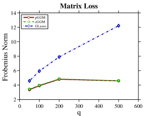
(a) Frobenius norm loss ($\downarrow$)

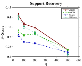
(b) Support recovery F-score ($\uparrow$)

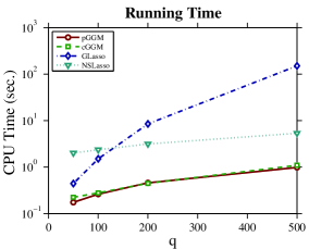
(c) CPU running time ($\downarrow$)

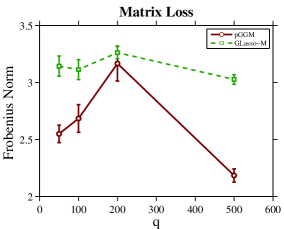
(d) Frobenius norm loss ($\downarrow$)

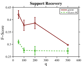
(e) Support recovery F-score ($\uparrow$)

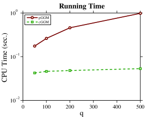
(f) CPU running time ($\downarrow$)

Figure 6.1: Performance curves on the synthetic data. Top row: comparison of the estimated blocks $\{\hat{\Omega}_{yy},\hat{\Omega}_{yx}\}$. Bottom row: comparison of the estimated $\hat{\Omega}_{yy}$ by pGGM and GLasso-M. The down-arrow $\downarrow$ means the smaller the better while the up-arrow $\uparrow$ means the larger the better.

We further compare pGGM to GLasso applied to the marginal distribution of $Y$ by ignoring $X$. We call this method as GLasso-M. The results are plotted in Figure 1(d), 1(e), 1(f). It can be observed from these figures that pGGM consistently outperforms GLasso-M in terms of parameter estimation and support recovery accuracies.

The detailed performance figures that are used to generate Figure 6.1 are presented in Appendix B in tabular forms, along with additional performance metrics in spectral norm and matrix $\ell_{1}$-norm. The observations using the other norms are consistent with that of the Frobenius norm.

6.2 Real Data

We further study the performance of pGGM on real data.

6.2.1 Data

We use three multi-label datasets Corel5k, MIRFlickr25k and RCV1-v2 and a stock price dataset S&P500 for this study. For each dataset, we generate a training sample for parameter estimation and an independent test sample for evaluation. Table 6.1 summarizes some statistics of the data. We next describe the derails of these datasets.

Corel5k. This dataset was first used in (Duygulu et al., 2002). Since then, it has become a standard benchmark for keyword based image retrieval and image annotation. It contains around 5,000 images manually annotated with 1 to 5 keywords. The vocabulary contains 260 visual words. The average number of keywords per sample is 3.4 and the maximum number of keywords per sample is 5. The data set along with the extracted visual features are publicly available at lear.inrialpes.fr/people/guillaumin/data.php. In our experiment, we down sample the training data to size 450 for constructing the Gaussian graphical models of image keywords. For evaluation purpose, an independent test set of size 450 is selected. Each image is described by the GIST feature which has dimensionality 512. Our goal is to construct a graphical model for image tags. Note that the size of label-feature joint variable is $260+512=772$, which allows us to examine the performance when $p+q>n$.

MIRFlickr25k. This data contains 25,000 images collected from Flickr over a period of 15 months. The database is available at press.liacs.nl/mirflickr/. The collection contains highest scored images according to Flickr’s “interestingness” score. These images were annotated for 24 concepts, including object categories but also more general scene elements such as sky, water or indoor. For 14 of the 24 concepts, a second and more strict annotation was made. The vocabulary contains 457 tags. The average number of words per sample is 2.7 and the maximum words per sample is 32. The data set along with the extracted visual features are publicly available at lear.inrialpes.fr/people/guillaumin/data.php. In our experiment, we down sample the training set to size 1,250 for constructing the Gaussian graphical models of image keywords. For evaluation purpose, an independent test set of size 1,250 is selected. Each image is described by the GIST feature of dimension 512. Our goal is to construct a graphical model for image tags.

RCV1-v2. This data set contains newswire stories from Reuters Ltd Lewis et al. (2004). Several schemes were utilized to process the documents including removing stopping words, stemming, and transforming each document into a numerical vector. There are three sets of categories: Topics, Industries and Regions. In this paper, we consider the Topics category set, and make use of a subset collection (sample size 3,000, feature dimension 47,236) of this data from www.csie.ntu.edu.tw/~cjlin/libsvmtools/datasets. We further down sample the data set to a size of 1,000, and select the top 1,000 words with highest TF-IDF frequencies. For evaluation purpose, an independent test set of size 1,000 is selected. The vocabulary contains 103 keywords. The average number of words per sample is 3.3 and the maximum words per sample is 12. Our goal is to construct a graphical models for these keywords.

S&P500. We investigate the historical prices of S&P500 stocks over 5 years, from January 1, 2007 to January 1, 2012. By taking out the stocks with less than 5 years of history, we end up with 465 stocks, each having daily closing prices over 1,260 trading days. The prices are first adjusted for dividends and splits and the used to calculate daily log returns. Each day’s return can be represented as a point in ${\mathbb{R}}^{465}$. For each day’s return, we chose the first 300 as $X$ and the rest $165$ as $Y$. We down sample the data set to size 101. For evaluation purpose, an independent test set of size 101 is selected. Our goal is to construct the conditional precision matrix of $Y$ conditioned on $X$.

Table 6.1: Statistics of data.

	$p$	$q$	training size (n)	test size
Corel5k	260	512	450	450
MIRFlickr25k	457	512	1,250	1,250
RCV1-v2	103	1,000	1,000	1,000
S&P500	165	300	101	101

Table 6.2: Quantitative results on real data

	$L_{\text{pa}}$ value on test set				CPU Time (sec.)on training set
	pGGM	GLasso	GLasso-M	NSLasso	pGGM	GLasso	GLasso-M	NSLasso
Corel5k	-1.08e3	-0.63e3	—	—	16.63	125.74	9.07	9.06
MIRFlickr25k	-1.99e3	-1.99e3	—	—	56.93	228.71	39.74	42.89
RCV1-v2	-0.42e3	-0.39e3	—	—	3.04	421.86	1.38	75.43
S&P500	0.22e3	0.24e3	—	—	4.83	46.65	4.28	4.29

6.2.2 Methods and Evaluation Metrics

In these experiments, we compare pGGM to GLasso, GLasso-M (for estimating marginal precision matrix using the data component $Y$ only) and NSLasso. Here we focus on convex formulations, and thus skip cGGM. For all these methods, we use the Bayesian information criterion (BIC) to select the regularization parameters.

Since there is no ground truth precision matrix, we measure the quality of $\hat{\Theta}$ by evaluating the $L_{\text{pa}}$ objective (recall its definition in (2.3)) on the test data. The training CPU times are also reported. Since the category information of RCV1-v2 and S&P500 are available, we also measure the precision of the top $k$ links in the constructed conditional GGM from $\Omega_{yy}$ on these two datasets. A link is regarded as true if and only if it connects two nodes belonging to the same category. Note that the category information is not used in any of the graphical model learning procedures.

6.2.3 Results

Table 6.2 tabulates the evaluated $L_{\text{pa}}$ objectives on the test set and the training time. The key observations are

• In most cases, pGGM outputs smaller $L_{\text{pa}}$ objective value than GLasso (note that the $L_{\text{pa}}$ value cannot be evaluated for GLasso-M and NSLasso). pGGM runs much faster than GLasso on all these datasets.

• pGGM is slightly slower than NSLasso on Corel5k, MIRFlickr25k and S&P500 where $p\sim q$, but significantly faster than NSLasso on RCV1-v2 where $p\ll q$.

Figure 6.2 shows the precision of top $k$ links in the conditional graphs as a function of $k$. It can be seen that pGGM performs favorably in comparison to the other three methods for identifying correct links on RCV1-v2. On S&P500, pGGM and GLasso-M have comparable performance, and both are better than GLasso and NSLasso. This is because the S&P500 stocks are weakly correlated and thus the conditional graphical model can be well approximated by the marginal graphical model.

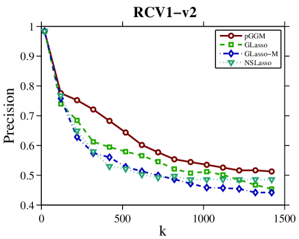
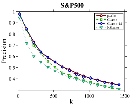
Figure 6.2: Link precision curves on RCV1-v2 and S&P500.

We further evaluate the sparsity of the constructed graphs on these datasets. The links are identified by $\{(i,j):i\neq j,|[\hat{\Omega}_{yy}]_{ij}|\geq\mu\}$ in which $\mu>0$ is a threshold value. Figure 6.3 shows the number of links in graphs as a function of $\mu$. It can be seen that pGGM, GLasso and NSLasso tend to output sparser graphical models than GLasso-M. A potential reason is that GLasso-M ignores the information provided by $X$, and thus false positive links can be induced. NSLasso outputs the sparsest network on corel5k, MIRFlickr25k and S&P500, while pGGM outputs the sparsest model on RCV1-v2. Note that NSLasso does not estimate precision matrix. Moreover, pGGM tends to be slightly sparser than GLasso. These observations are consistent with our observations on the synthetic data.

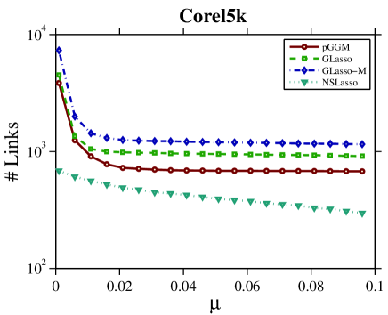
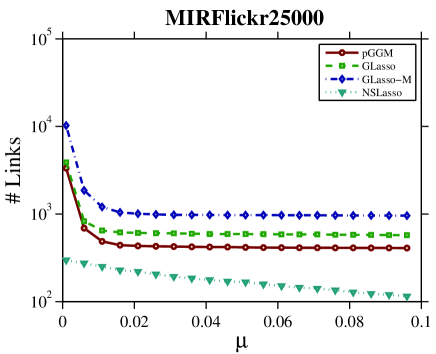
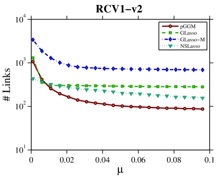
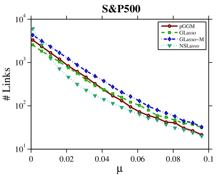
Figure 6.3: Number of links as a function of $\mu$ in the constructed conditional graphical model.

Figure 6.4 plots the graphs constructed by using different estimation methods with $\mu=0.1$ for Corel5k, MIRFlickr25k and RCV1-v2, and $\mu=0.05$ for S&P500. It can be seen that different methods will construct different graphs. Figure 6.5 illustrates in detail the top 50 links in each graph.

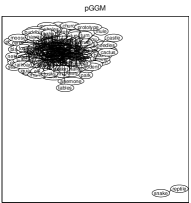
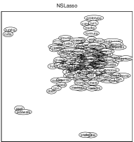
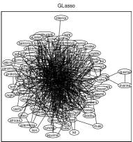
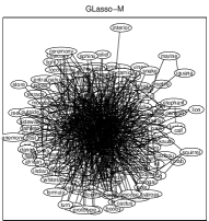
(a) Corel5k, $\mu=0.1$. Method(# Links): pGGM (677), NSLasso (293), GLasso (909), GLasso-M (1153).

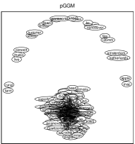
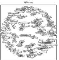
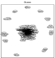
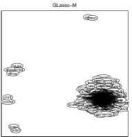
(b) MIRFlicker25k, $\mu=0.1$. Method(# Links): pGGM (409), NSLasso (110), GLasso (573), GLasso-M (960).

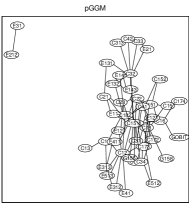
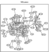
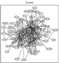
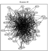
(c) RCV1-v2, $\mu=0.1$. Method(# Links): pGGM (87), NSLasso (156), GLasso (282), GLasso-M (688).

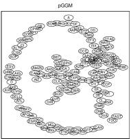
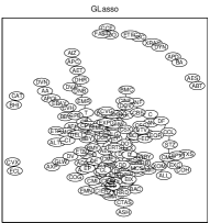
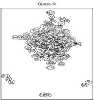
(d) S&P500, $\mu=0.05$. Method(# Links): pGGM (136), NSLasso (94), GLasso (160), GLasso-M (221).

Figure 6.4: Constructed graphs by pGGM, NSLasso, GLasso and GLasso-M.

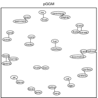
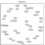
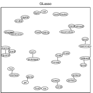
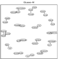
(a) Corel5k.

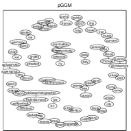
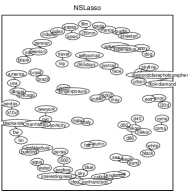
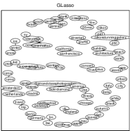
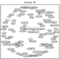
(b) MIRFlicker25k.

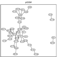
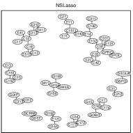
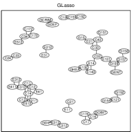
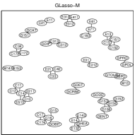
(c) RCV1-v2.

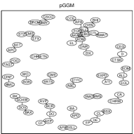
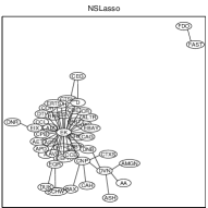
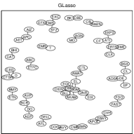
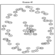
(d) S&P500.

Figure 6.5: The top 50 links in the constructed graphs by pGGM, NSLasso, GLasso and GLasso-M.

7 Conclusion

This paper presents a new formulation pGGM for estimating sparse partial precision matrix. The advantages of pGGM over prior GGMs and conditional GGMs include: (i) the formulation is convex; (ii) the optimization procedure scales well with respect to the component $X$; (iii) the model has natural interpretation in terms of the conditional dependency between the variables in $X$ and $Y$; and (iv) theoretical guarantees on the global solution can be established without sparsity assumptions on the precision matrix of $X$. We showed that the rate of convergence of pGGM depends on how sparse the underlying true partial precision matrix is. Numerical experiments on several synthetic and real datasets demonstrated the competitive performance of pGGM compared to the existing approaches.

In the current paper, the pGGM is derived under the assumption that $(Y;X)$ is jointly normally distributed. As discussed in Section 5 that pGGM is still valid in the setting where the joint normality is relaxed to the conditional normality. We would like to point out that by assuming the Gaussian copular structure of the random vector, pGGM can be easily extended to the setting of nonparanormal (Liu et al., 2009) which is a useful tool for semiparametric estimation of high dimensional undirected graphs. We believe that such an extension will broaden the application range of pGGM in practice.

Appendix A Technical Proofs

A.1 Proof of Proposition 1

Proof.

Using the following well known fact of block matrix determinant

$$\det\left(\left[{{\begin{array}[]{*{20}{c}}{A}&{B^{\top}}\\ {B}&{C}\\ \end{array}}}\right]\right)=\det(A)\det(C-BA^{-1}B^{\top})$$

and simple algebra, we obtain that

$$L(\Omega_{yy},\Omega_{yx},\Omega_{xx})=L_{\text{pa}}(\Omega_{yy},\Omega_{yx})-\log\det(\Omega_{xx}-\Omega_{yx}^{\top}\Omega_{yy}^{-1}\Omega_{yx})+\mathrm{tr}(\Sigma^{n}_{xx}(\Omega_{xx}-\Omega_{yx}^{\top}\Omega_{yy}^{-1}\Omega_{yx})),$$ (A.1)

where

$$L_{\text{pa}}(\Omega_{yy},\Omega_{yx})=-\log\det(\Omega_{yy})+\mathrm{tr}(\Sigma^{n}_{yy}\Omega_{yy})+2\mathrm{tr}(\Sigma^{n\top}_{yx}\Omega_{yx})+\mathrm{tr}(\Sigma^{n}_{xx}\Omega_{yx}^{\top}\Omega_{yy}^{-1}\Omega_{yx}).$$

The claim (2.2) follows immediately from the re-parametrization of $\tilde{\Omega}_{xx}=\Omega_{xx}-\Omega_{yx}^{\top}\Omega_{yy}^{-1}\Omega_{yx}$.

We next show that $L_{\text{pa}}(\Omega_{yy},\Omega_{yx})$ is convex. Note that when $\Sigma_{xx}^{n}\succ 0$, by minimizing both sides of (A.1) over $\Omega_{xx}$, which is achieved at $\Omega_{xx}=(\Sigma_{xx}^{n})^{-1}+\Omega_{yx}^{\top}\Omega_{yy}^{-1}\Omega_{yx}$, we know that up to an additive constant, $L_{\text{pa}}$ is the pointwise minimum of $L$ over $\Omega_{xx}$. Since the pointwise minimization of a convex objective function with a part of the parameters is convex with respect to the other parameters (see, e.g., Boyed & Vandenberghe, 2004), we immediately obtain the convexity of $L_{\text{pa}}$. In the high-dimensional case where $n<q$, we only have $\Sigma^{n}_{xx}\succeq 0$ and thus the minimization over $\Omega_{xx}$ is not well-defined. To show the convexity in general case, we may replace $\Sigma_{xx}$ by $\Sigma_{xx}+\lambda I$ for some $\lambda>0$, and the resulting partial GMM formula:

$$L_{\text{pa}}^{\lambda}(\Omega_{yy},\Omega_{yx})=-\log\det(\Omega_{yy})+\mathrm{tr}(\Sigma^{n}_{yy}\Omega_{yy})+2\mathrm{tr}(\Sigma^{n\top}_{yx}\Omega_{yx})+\mathrm{tr}((\Sigma^{n}_{xx}+\lambda I)\Omega_{yx}^{\top}\Omega_{yy}^{-1}\Omega_{yx})$$

is convex in $(\Omega_{yy},\Omega_{yx})$ by the previous argument. Now, let $\lambda\to 0^{+}$, we have $L_{\text{pa}}^{\lambda}(\Omega_{yy},\Omega_{yx})\to L_{\text{pa}}(\Omega_{yy},\Omega_{yx})$, which immediately implies the convexity of $L_{\text{pa}}(\cdot,\cdot)$. ∎

A.2 Proof of Proposition 3

Lemma 1.

Assume the conditions of the proposition hold. Then for any matrix $V=(V_{yy},V_{yx})\in{\mathbb{R}}^{p\times p}\times{\mathbb{R}}^{p\times q}$ such that $|V_{\bar{S}}|_{1}\leq\alpha|V_{S}|_{1}$, we have

$$\mathrm{tr}(V\tilde{\Sigma}V^{\top})\geq\frac{\rho_{-}}{5}\|V\|_{F}^{2},\qquad\text{ where }\quad\tilde{\Sigma}=\left[\begin{array}[]{cc}\Omega_{yy}^{-1}&0\\ 0&\Sigma^{n}_{xx}\end{array}\right].$$

Moreover, we have

$$\mathrm{tr}(V_{yx}\Sigma^{n}_{xx}V_{yx}^{\top})\leq 2.25\rho_{+}\|V\|_{F}^{2}.$$

Proof.

In the following, we let $s=|S|$ and $s^{\prime}=\tilde{s}-s\geq 4(\rho_{+}/\rho_{-})\alpha^{2}s$. Since $r\leq\lambda_{\max}(\Omega^{*}_{yy})$, we know that $\lambda_{\max}(\Omega_{yy})^{-1}\geq\rho_{-}$. Indeed, $\lambda_{\max}(\Omega_{yy})\leq\lambda_{\max}(\Omega^{*}_{yy})+\lambda_{\max}(\Delta\Omega_{yy})\leq\lambda_{\max}(\Omega^{*}_{yy})+r\leq 2\lambda_{\max}(\Omega^{*}_{yy})$, which from the definition of $\rho^{-}$ implies that $\lambda_{\max}(\Omega_{yy})^{-1}\geq\rho_{-}$. Therefore for any $U\in{\mathbb{R}}^{p\times(p+q)}$ such that $|U|_{0}\leq s+s^{\prime}$, the conditions of Assumption 1 imply that

$$\mathrm{tr}(U\tilde{\Sigma}U^{\top})\geq\rho_{-}\|U\|_{F}^{2}.$$

We order the elements of $V_{\bar{S}}$ in descending order of absolute values. Let $V^{(0)}=V_{S}$ which contains $s$ nonzero values, and $V^{(k)}$ contains (at most) $s^{\prime}$ nonzero values of $V_{\bar{S}}$ with $(ks^{\prime}-s^{\prime}+1)$-th to $(ks^{\prime})$-th largest absolute values. It follows that $\|V^{(k+1)}\|_{F}\leq\sqrt{|V^{(k+1)}|_{\infty}|V^{(k+1)}|_{1}}\leq|V^{(k)}|_{1}/\sqrt{s^{\prime}}$ for all $k\geq 1$. Therefore we have

$$a_{0}=\mathrm{tr}((V^{(0)}+V^{(1)})\tilde{\Sigma}(V^{(0)}+V^{(1)})^{\top})\geq\rho_{-}\|V^{(0)}+V^{(1)}\|_{F}^{2}$$

and

$$a_{1}= \big{|}\mathrm{tr}((V^{(0)}+V^{(1)})\tilde{\Sigma}\sum_{k\geq 1}V^{(k+1)\top})\big{|}$$

$$\leq \sqrt{a_{0}}\sqrt{\rho_{+}}\sum_{k\geq 1}\|V^{(k+1)}\|_{F}$$

$$\leq \sqrt{a_{0}\rho_{+}}\sum_{k\geq 1}|V^{(k)}|_{1}/\sqrt{s^{\prime}}$$

$$\leq \alpha\sqrt{a_{0}\rho_{+}}|V_{S}|_{1}/\sqrt{s^{\prime}}\leq\alpha\sqrt{a_{0}\rho_{+}}\|V^{(0)}+V^{(1)}\|_{F}\sqrt{s/s^{\prime}}.$$

Note that $\mathrm{tr}(V\tilde{\Sigma}V^{\top})\geq a_{0}-2a_{1}+a_{2}$, where

$$a_{2}=\mathrm{tr}\left(\left(\sum_{k\geq 1}V^{(k+1)}\right)\tilde{\Sigma}\left(\sum_{k\geq 1}V^{(k+1)}\right)^{\top}\right).$$

The semi-positive-definiteness of $\tilde{\Sigma}$ implies that $\min_{\mu}[a_{0}+2\mu a_{1}+\mu^{2}a_{2}]\geq 0$, which implies that $a_{1}^{2}\leq a_{0}a_{2}$. Therefore

$$\mathrm{tr}(V^{\top}\tilde{\Sigma}V)\geq a_{0}-2a_{1}+a_{2}\geq a_{0}-2a_{1}+a_{1}^{2}/a_{0}$$

$$\geq \rho_{-}\|V^{(0)}+V^{(1)}\|_{F}^{2}(1-\alpha\sqrt{(\rho_{+}/\rho_{-})(s/s^{\prime})})^{2}\geq\rho_{-}\|V^{(0)}+V^{(1)}\|_{F}^{2}/4,$$

where the last inequality is due to the definition of $s^{\prime}$ that implies that $\alpha\sqrt{(\rho_{+}/\rho_{-})(s/s^{\prime})}\leq 0.5$.

Moreover we have

$$\|V\|_{F}^{2}= \|V^{(0)}+V^{(1)}\|_{F}^{2}+\sum_{k\geq 1}\|V^{(k+1)}\|_{F}^{2}$$

$$\leq \|V^{(0)}+V^{(1)}\|_{F}^{2}+\sum_{k\geq 1}\|V^{(k)}\|_{1}^{2}/s^{\prime}$$

$$\leq \|V^{(0)}+V^{(1)}\|_{F}^{2}+\|V^{(1)}\|_{1}\|V_{\bar{S}}\|_{1}/s^{\prime}$$

$$\leq \|V^{(0)}+V^{(1)}\|_{F}^{2}+\alpha\|V^{(1)}\|_{2}\|V_{S}\|_{2}\sqrt{s/s^{\prime}}$$

$$\leq (1+0.5\alpha\sqrt{s/s^{\prime}})\|V^{(0)}+V^{(1)}\|_{F}^{2}\leq 1.25\|V^{(0)}+V^{(1)}\|_{F}^{2}.$$

By combining the previous two displayed inequalities, we obtain the first desired bound.

To prove the second bound, we define

$$\tilde{\Sigma}^{\prime}=\left[\begin{array}[]{cc}0_{p\times p}&0\\ 0&\Sigma^{n}_{xx}\end{array}\right].$$

Therefore for any $U\in{\mathbb{R}}^{p\times(p+q)}$ such that $|U|_{0}\leq s+s^{\prime}$, the conditions of Assumption 1 imply that

$$\mathrm{tr}(U\tilde{\Sigma}^{\prime}U^{\top})\leq\rho_{+}\|U\|_{F}^{2}.$$

Therefore we have

$$a_{0}^{\prime}=\mathrm{tr}((V^{(0)}+V^{(1)})\tilde{\Sigma}^{\prime}(V^{(0)}+V^{(1)})^{\top})\leq\rho_{+}\|V\|_{F}^{2}$$

and

$$a_{2}^{\prime}= \mathrm{tr}\left(\left(\sum_{k\geq 1}V^{(k+1)}\right)\tilde{\Sigma}^{\prime}\left(\sum_{k\geq 1}V^{(k+1)}\right)^{\top}\right)$$

$$\leq \sum_{k\geq 1}\sum_{k^{\prime}\geq 1}\mathrm{tr}(V^{(k+1)}\tilde{\Sigma}^{\prime}V^{(k^{\prime}+1)\top})$$

$$\leq \rho_{+}\sum_{k\geq 1}\sum_{k^{\prime}\geq 1}\|V^{(k+1)}\|_{F}\|V^{(k^{\prime}+1)}\|_{F}$$

$$\leq \rho_{+}\sum_{k\geq 1}\sum_{k^{\prime}\geq 1}|V^{(k)}|_{1}|V^{(k^{\prime})}|_{1}/s^{\prime}\leq\rho_{+}|V_{\bar{S}}|_{1}^{2}/s^{\prime}$$

$$\leq \alpha^{2}\rho_{+}|V_{S}|_{1}^{2}/s^{\prime}\leq\alpha^{2}\rho_{+}\|V\|_{F}^{2}(s/s^{\prime}).$$

Therefore we obtain (using $\alpha^{2}(s/s^{\prime})\leq 0.25$)

$$\mathrm{tr}(V_{yx}\Sigma^{n}_{xx}V_{yx}^{\top})\leq a_{0}^{\prime}+2\sqrt{a_{0}^{\prime}a_{2}^{\prime}}+a_{2}^{\prime}\leq 1.5a_{0}^{\prime}+3a_{2}^{\prime}\leq(1.5+3/4)\rho_{+}\|V\|_{F}^{2}=2.25\|V\|_{F}^{2}.$$

This completes the proof. ∎

Lemma 2.

Let

$$\vartheta=\min\left[\frac{2}{3},\frac{\lambda_{\min}(\Omega^{*}_{yy})}{8\lambda_{\max}(\Omega^{*}_{yx}\Sigma^{*}_{xx}(\Omega^{*}_{yx})^{\top})}\right],$$

then we have

$$\lambda_{\max}(\Omega_{yy}^{-1}\Omega_{yx}\Sigma^{n}_{xx}\Omega_{yx}^{\top})\leq 1/(2\vartheta).$$

Proof.

Let $\sigma(A)$ be the largest singular value of a matrix $A$, then $\sigma(A)=\sqrt{\lambda_{\max}(A^{\top}A)}$. Therefore we have

$$\sqrt{\lambda_{\max}\big{[}\Omega_{yx}\Sigma^{n}_{xx}\Omega_{yx}^{\top}\big{]}}= \sigma(\Omega_{yx}(\Sigma^{n}_{xx})^{1/2})$$

$$\leq \sigma(\Omega^{*}_{yx}(\Sigma^{n}_{xx})^{1/2})+\sigma(\Delta\Omega_{yx}(\Sigma^{n}_{xx})^{1/2})$$

$$\leq \sigma(\Omega^{*}_{yx}(\Sigma^{n}_{xx})^{1/2})+\sqrt{\mathrm{tr}(\Delta\Omega_{yx}\Sigma^{n}_{xx}\Delta\Omega_{yx}^{\top})}$$

$$\leq \sqrt{\lambda_{\max}\big{[}\Omega^{*}_{yx}\Sigma^{n}_{xx}(\Omega^{*}_{yx})^{\top}\big{]}}+1.5\sqrt{\rho_{+}}\|\Delta\Omega\|_{F}$$

$$\leq 1.4\sqrt{\lambda_{\max}\big{[}\Omega^{*}_{yx}\Sigma^{*}_{xx}(\Omega^{*}_{yx})^{\top}\big{]}},$$

where the third inequality uses the second inequality of Lemma 1, and the last inequality uses the third inequality of Assumption 1 and $\|\Delta\Omega\|_{F}\leq r\leq 0.13\sqrt{\lambda_{\max}\big{[}\Omega^{*}_{yx}\Sigma^{*}_{xx}(\Omega^{*}_{yx})^{\top}\big{]}/\rho_{+}}$. This implies

$$\lambda_{\max}\big{[}\Omega_{yx}\Sigma^{n}_{xx}\Omega_{yx}^{\top}\big{]}\leq 2\lambda_{\max}\big{[}\Omega^{*}_{yx}\Sigma^{*}_{xx}(\Omega^{*}_{yx})^{\top}\big{]}.$$

Since the assumption of $r\leq\lambda_{\min}(\Omega^{*}_{yy})/2$ also implies that

$$\lambda_{\min}(\Omega_{yy})\geq\lambda_{\min}(\Omega^{*}_{yy})-\lambda_{\min}(\Delta\Omega_{yy})\geq\lambda_{\min}(\Omega^{*}_{yy})-r\geq\lambda_{\min}(\Omega^{*}_{yy})/2.$$

Therefore we have

$$\lambda_{\max}(\Omega_{yy}^{-1}\Omega_{yx}\Sigma^{n}_{xx}\Omega_{yx}^{\top})\leq\frac{\lambda_{\max}(\Omega_{yx}\Sigma^{n}_{xx}\Omega_{yx}^{\top})}{\lambda_{\min}(\Omega_{yy})}\leq\frac{4\lambda_{\max}\big{[}\Omega^{*}_{yx}\Sigma^{*}_{xx}(\Omega^{*}_{yx})^{\top}\big{]}}{\lambda_{\min}(\Omega^{*}_{yy})}=1/(2\vartheta),$$

which leads to the desired bound. ∎

Proof of Proposition 3.

For any $s\in(0,1)$, we define for convenience that

$$\Omega_{yy}=\Omega^{*}_{yy}+s\Delta\Omega_{yy},\quad\Omega_{yx}=\Omega^{*}_{yx}+s\Delta\Omega_{yx},$$

and consider the function $f(s)$ defined as

$$f(s):=-\log\det(\Omega_{yy})+\mathrm{tr}(\Sigma^{n}_{yy}\Omega_{yy})+2\mathrm{tr}(\Sigma^{n\top}_{yx}\Omega_{yx})+\mathrm{tr}(\Sigma^{n}_{xx}\Omega_{yx}^{\top}\Omega_{yy}^{-1}\Omega_{yx}).$$

It can be verified that

$$f^{\prime}(s)= -\mathrm{tr}(\Omega_{yy}^{-1}\Delta{\Omega}_{yy})+\mathrm{tr}(\Sigma^{n}_{yy}\Delta\Omega_{yy})$$

$$+2\mathrm{tr}(\Sigma^{n\top}_{yx}\Delta\Omega_{yx})+2\mathrm{tr}(\Sigma^{n}_{xx}\Omega_{yx}^{\top}\Omega_{yy}^{-1}\Delta\Omega_{yx})-\mathrm{tr}(\Sigma^{n}_{xx}\Omega_{yx}^{\top}\Omega_{yy}^{-1}\Delta\Omega_{yy}\Omega_{yy}^{-1}\Omega_{yx})$$

and

$$f^{\prime\prime}(s)= \mathrm{tr}(\Omega_{yy}^{-1}\Delta{\Omega}_{yy}\Omega_{yy}^{-1}\Delta{\Omega}_{yy})+2\mathrm{tr}(\Sigma^{n}_{xx}\Delta\Omega_{yx}^{\top}\Omega_{yy}^{-1}\Delta\Omega_{yx})-4\mathrm{tr}(\Sigma^{n}_{xx}\Omega_{yx}^{\top}\Omega_{yy}^{-1}\Delta\Omega_{yy}\Omega_{yy}^{-1}\Delta\Omega_{yx})$$

$$+2\mathrm{tr}(\Sigma^{n}_{xx}\Omega_{yx}^{\top}\Omega_{yy}^{-1}\Delta\Omega_{yy}\Omega_{yy}^{-1}\Delta\Omega_{yy}\Omega_{yy}^{-1}\Omega_{yx}).$$

We obtain from Taylor expansion that

$$\Delta L_{\text{pa}}(\Theta^{*},\Delta\Theta)=\frac{1}{2}f^{\prime\prime}(s),\quad\text{for some }s\in(0,1).$$

This implies that

$$f^{\prime\prime}(s) = \mathrm{tr}(\Omega_{yy}^{-1}\Delta\Omega_{yy}\Omega_{yy}^{-1}\Delta\Omega_{yy})+2\mathrm{tr}(\Sigma^{n}_{xx}\Delta\Omega^{\top}_{yx}\Omega^{-1}_{yy}\Delta\Omega_{yx})-4\mathrm{tr}(\Sigma^{n}_{xx}\Omega^{\top}_{yx}\Omega^{-1}_{yy}\Delta\Omega_{yy}\Omega_{yy}^{-1}\Delta\Omega_{yx})$$

$$+2\mathrm{tr}(\Sigma_{xx}^{n}\Omega^{\top}_{yx}\Omega_{yy}^{-1}\Delta\Omega_{yy}\Omega^{-1}_{yy}\Delta\Omega_{yy}\Omega_{yy}^{-1}\Omega_{yx})$$

$$= \mathrm{tr}(\Omega_{yy}^{-1}\Delta\Omega_{yy}\Omega_{yy}^{-1}\Delta\Omega_{yy})+2\mathrm{tr}(\Sigma^{n}_{xx}\Delta\Omega^{\top}_{yx}\Omega^{-1}_{yy}\Delta\Omega_{yx})-4\mathrm{tr}(\Sigma^{n}_{xx}\Omega^{\top}_{yx}\Omega^{-1}_{yy}\Delta\Omega_{yy}\Omega_{yy}^{-1}\Delta\Omega_{yx})$$

$$+(2+\vartheta)\mathrm{tr}(\Sigma_{xx}^{n}\Omega^{\top}_{yx}\Omega_{yy}^{-1}\Delta\Omega_{yy}\Omega^{-1}_{yy}\Delta\Omega_{yy}\Omega_{yy}^{-1}\Omega_{yx})-\vartheta\mathrm{tr}(\Sigma_{xx}^{n}\Omega^{\top}_{yx}\Omega_{yy}^{-1}\Delta\Omega_{yy}\Omega^{-1}_{yy}\Delta\Omega_{yy}\Omega_{yy}^{-1}\Omega_{yx})$$

$$\geq \mathrm{tr}(\Omega_{yy}^{-1}\Delta\Omega_{yy}\Omega_{yy}^{-1}\Delta\Omega_{yy})+\frac{2\vartheta}{2+\vartheta}\mathrm{tr}(\Sigma^{n}_{xx}\Delta\Omega^{\top}_{yx}\Omega^{-1}_{yy}\Delta\Omega_{yx})$$

$$-\vartheta\mathrm{tr}(\Omega_{yy}^{-1/2}\Omega_{yx}\Sigma_{xx}^{n}\Omega^{\top}_{yx}\Omega_{yy}^{-1/2}\;\Omega_{yy}^{-1/2}\Delta\Omega_{yy}\Omega^{-1}_{yy}\Delta\Omega_{yy}\Omega_{yy}^{-1/2})$$

$$\geq \mathrm{tr}(\Omega_{yy}^{-1}\Delta\Omega_{yy}\Omega_{yy}^{-1}\Delta\Omega_{yy})+\frac{2\vartheta}{2+\vartheta}\mathrm{tr}(\Sigma^{n}_{xx}\Delta\Omega^{\top}_{yx}\Omega^{-1}_{yy}\Delta\Omega_{yx})$$

$$-\vartheta\lambda_{\max}(\Omega_{yy}^{-1/2}\Omega_{yx}\Sigma_{xx}^{n}\Omega^{\top}_{yx}\Omega_{yy}^{-1/2})\mathrm{tr}(\Omega_{yy}^{-1/2}\Delta\Omega_{yy}\Omega^{-1}_{yy}\Delta\Omega_{yy}\Omega_{yy}^{-1/2})$$

$$\geq 0.5\mathrm{tr}(\Omega_{yy}^{-1}\Delta\Omega_{yy}\Omega_{yy}^{-1}\Delta\Omega_{yy})+\frac{2\vartheta}{2+\vartheta}\mathrm{tr}(\Sigma^{n}_{xx}\Delta\Omega^{\top}_{yx}\Omega^{-1}_{yy}\Delta\Omega_{yx}),$$

where we have used the trace equality $\mathrm{tr}(AB)=\mathrm{tr}(BA)$ throughout the derivations. The first inequality is due to the trace inequality $(2/(2+\vartheta))\mathrm{tr}(A^{\top}A)-4\mathrm{tr}(A^{\top}B)+(2+\vartheta)\mathrm{tr}(B^{\top}B)\geq 0$; the second inequality uses $\mathrm{tr}(AB)\leq\lambda_{\max}(A)\mathrm{tr}(B)$ for symmetric positive semidefinite matrices $A$ and $B$; and the last inequality is due to $\lambda_{\max}(\Omega_{yy}^{-1/2}\Omega_{yx}\Sigma^{n}_{xx}\Omega_{yx}^{\top}\Omega_{yy}^{-1/2})\vartheta\leq 1/2$ (Lemma 2).

Since $\vartheta\leq 2/3$, we have $0.5\geq 2\vartheta/(2+\vartheta)$. Therefore

$$2\Delta L_{\text{pa}}(\Theta^{*},\Delta\Theta)= f^{\prime\prime}(s)$$

$$\geq \frac{2\vartheta}{2+\vartheta}\left[\mathrm{tr}(\Omega_{yy}^{-1}\Delta\Omega_{yy}\Omega_{yy}^{-1}\Delta\Omega_{yy})+\mathrm{tr}(\Sigma^{n}_{xx}\Delta\Omega^{\top}_{yx}\Omega^{-1}_{yy}\Delta\Omega_{yx})\right]$$

$$\geq \frac{2\vartheta}{2+\vartheta}\lambda_{\max}^{-1}(\Omega_{yy})\left[\mathrm{tr}(\Delta\Omega_{yy}\Omega_{yy}^{-1}\Delta\Omega_{yy})+\mathrm{tr}(\Delta\Omega_{yx}\Sigma^{n}_{xx}\Delta\Omega^{\top}_{yx})\right]$$

$$\geq \frac{2\vartheta\lambda_{\max}^{-1}(\Omega_{yy})\rho_{-}}{5(2+\vartheta)}\|\Delta\Theta\|_{F}^{2},$$

where the second inequality uses $\mathrm{tr}(AB)\geq\lambda_{\min}(A)\mathrm{tr}(B)$ for symmetric positive semidefinite matrices $A$ and $B$; and the last inequality follows from Lemma 1. We complete the proof by noticing $5(2+\vartheta)\leq 40/3$. ∎

A.3 Proof of Proposition 4

We will employ the following tail-bound for $\chi^{2}$ random variable, due to Laurent & Massart (2000).

Lemma 3.

Consider independent Gaussian random variables $z_{1},\ldots,z_{n}\sim\mathcal{N}(0,\sigma^{2})$. We have for all $t>0$:

$$\Pr\left[\sum_{\ell=1}^{n}z_{\ell}^{2}\geq n\sigma^{2}+2\sigma^{2}\sqrt{nt}+2\sigma^{2}t\right]\leq e^{-t}$$

and

$$\Pr\left[\sum_{\ell=1}^{n}z_{\ell}^{2}\leq n\sigma^{2}-2\sigma^{2}\sqrt{nt}\right]\leq e^{-t}.$$

The following lemma is a consequence of Lemma 3 when applied to the covariance of multivariate Gaussian distribution.

Lemma 4.

Consider the covariance matrix $\Sigma^{*}$ of a $d$-dimensional Gaussian random vector and its sample covariance $\Sigma^{n}$ from $n$ i.i.d. Gaussian random vectors from $\mathcal{N}(0,\Sigma^{*})$. For any $\eta\in(0,1)$ and any deterministic $d^{\prime}\times d$ matrix $A$. Let

$$\sigma^{2}=\max_{ij}\left[(A\Sigma^{*}A^{\top})_{ii}+2|(A\Sigma^{*})_{ij}|+(\Sigma^{*})_{jj}\right],$$

then with probability at least $1-\eta$ for any $\eta\in(0,1)$, we have

$$|A(\Sigma^{n}-\Sigma^{*})|_{\infty}\leq 2\sigma^{2}\sqrt{\ln(4dd^{\prime}/\eta)/n},$$

provided that $n\geq\ln(4dd^{\prime}/\eta)$.

Proof.

Consider the multivariate Gaussian random vector $X^{(1)},\dots,X^{(n)}\sim{\mathcal{N}}(0,\Sigma^{*})$.

Given any index pair $(i,j)$, let $z^{(\ell)}=(AX^{(\ell)})_{i}+X^{(\ell)}_{j}$. We have $z^{(\ell)}\sim{\mathcal{N}}(0,(A\Sigma^{*}A^{\top})_{ii}+2(A\Sigma^{*})_{ij}+(\Sigma^{*})_{jj})$. We thus obtain from Lemma 3 that for $t\leq n$: with probability at least $1-2e^{-t}$,

$$\left|n^{-1}\sum_{\ell=1}^{n}(AX^{(\ell)})_{i}+X^{(\ell)}_{j})^{2}-[(A\Sigma^{*}A^{\top})_{ii}+2(A\Sigma^{*})_{ij}+(\Sigma^{*})_{jj}]\right|\leq 4\sigma^{2}\sqrt{t/n}.$$

Similarly, we have for $t\leq n$: with probability at least $1-2e^{-t}$,

$$\left|n^{-1}\sum_{\ell=1}^{n}(AX^{(\ell)})_{i}-X^{(\ell)}_{j})^{2}-[(A\Sigma^{*}A^{\top})_{ii}-2(A\Sigma^{*})_{ij}+(\Sigma^{*})_{jj}]\right|\leq 4\sigma^{2}\sqrt{t/n}.$$

Taking union bound, and adding the previous two inequalities, we obtain that with probability at least $1-4e^{-t}$:

$$\left|\left[n^{-1}\sum_{\ell=1}^{n}(AX^{(\ell)})_{i}+X^{(\ell)}_{j})^{2}-[(A\Sigma^{*}A^{\top})_{ii}+2(A\Sigma^{*})_{ij}+(\Sigma^{*})_{jj}]\right]\right.$$

$$\left.-\left[n^{-1}\sum_{\ell=1}^{n}(AX^{(\ell)})_{i}-X^{(\ell)}_{j})^{2}-[(A\Sigma^{*}A^{\top})_{ii}-2(A\Sigma^{*})_{ij}+(\Sigma^{*})_{jj}]\right]\right|\leq 8\sigma^{2}\sqrt{t/n}.$$

This simplifies to $|A(\Sigma^{n}-\Sigma^{*})_{ij}|\leq 2\sigma^{2}\sqrt{t/n}$. Now by taking union bound over $i=1,\ldots,d^{\prime}$ and $j=1,\ldots,d$, and set $\eta=4dd^{\prime}e^{-t}$, we obtain the desired bound. ∎

Note that in Lemma 4, we have $\sigma^{2}\leq 2\max_{i}(A\Sigma^{*}A^{\top})_{ii}+2\max_{i}(\Sigma^{*})_{ii}$. It implies that with probability $1-\eta$:

$$|A(\Sigma^{n}-\Sigma^{*})|_{\infty}\leq 4[\max_{i}(A\Sigma^{*}A^{\top})_{ii}+\max_{i}(\Sigma^{*})_{ii}]\sqrt{\ln(4dd^{\prime}/\eta)/n}$$ (A.2)

when $n\geq\ln(4dd^{\prime}/\eta)$.

Proof of Proposition 4.

For any $\eta\in(0,1)$ such that $n\geq\ln(10(p+q)^{2}/\eta)$, we obtain from (A.2) with $A=I$ that with probability $1-0.4\eta$:

$$|\Sigma^{n}-\Sigma^{*}|_{\infty}\leq 8\max_{i}(\Sigma^{*})_{ii}\sqrt{\ln(10(p+q)^{2}/\eta)/n}.$$

Let $\tilde{A}=(\Omega^{*}_{yy})^{-1}\Omega^{*}_{yx}$. We may also apply (A.2) to the Gaussian covariance matrix $\tilde{A}\Sigma^{*}_{xx}\tilde{A}^{\top}$ and $A=I$ to obtain that with probability $1-0.4\eta$:

$$|\tilde{A}\Sigma^{n}_{xx}\tilde{A}^{\top}-\tilde{A}\Sigma^{*}_{xx}\tilde{A}^{\top}|_{\infty}\leq 8\max_{i}(\tilde{A}\Sigma^{*}_{xx}\tilde{A}^{\top})_{ii}\sqrt{\ln(10q^{2}/\eta)/n}.$$

Similarly, we may also apply (A.2) to the Gaussian covariance matrix $\Sigma^{*}$ with $A=\tilde{A}$ to obtain that with probability $1-0.2\eta$:

$$|\tilde{A}\Sigma^{n}_{xx}-\tilde{A}\Sigma^{*}_{xx}|_{\infty}\leq 8\max_{i}(\tilde{A}\Sigma^{*}_{xx}\tilde{A}^{\top})_{ii}\sqrt{\ln(20pq/\eta)/n}.$$

Taking union bound with the previous three inequalities, we have with probability $1-\eta$:

$$A_{n}\leq|\Sigma^{n}-\Sigma^{*}|_{\infty}+|\tilde{A}\Sigma^{n}_{xx}\tilde{A}^{\top}-\tilde{A}\Sigma^{*}_{xx}\tilde{A}^{\top}|_{\infty}\leq 8K_{*}\sqrt{\ln(10(p+q)^{2}/\eta)/n}$$

and

$$0.5B_{n}\leq|\Sigma^{n}-\Sigma^{*}|_{\infty}+|\tilde{A}\Sigma^{n}_{xx}-\tilde{A}\Sigma^{*}_{xx}|_{\infty}\leq 8K_{*}\sqrt{\ln(10(p+q)^{2}/\eta)/n},$$

where

$$K_{*}=\max_{i}(\Sigma^{*}_{ii})+\max_{i}(((\Omega^{*}_{yy})^{-1}\Omega^{*}_{yx}\Sigma^{*}_{xx}\Omega^{*\top}_{yx}(\Omega^{*}_{yy})^{-1})_{ii}).$$

This completes the proof. ∎

A.4 Proof of Theorem 1

For convenience, we will introduce the following notations:

$$\Delta\Omega_{yy}:=\hat{\Omega}_{yy}-\Omega^{*}_{yy},\qquad\Delta\Omega_{yx}:=\hat{\Omega}_{yx}-\Omega^{*}_{yx},$$

and $\Delta\Theta=\hat{\Theta}-\Theta^{*}=(\Delta\Omega_{yy},\Delta\Omega_{yx})$.

We first introduce the following lemma which shows that error is in the cone of Definition 1.

Lemma 5.

Assume that $\min\{\lambda_{n},\rho_{n}\}\geq 2\gamma_{n}$. Then the error $\Delta\Theta$ satisfies $|\Delta\Theta_{\bar{S}}|_{1}\leq\alpha|\Delta\Theta_{S}|_{1}$.

Proof.

Since $(\Omega^{*}_{yy})_{\bar{S}_{yy}}=0$, we have

$$|(\Omega^{*}_{yy}+\Delta\Omega_{yy})^{-}|_{1}-|(\Omega^{*}_{yy})^{-}|_{1} = |(\Omega^{*}_{yy}+\Delta\Omega_{yy})^{-}_{S_{yy}}|_{1}+|(\Omega^{*}_{yy}+\Delta\Omega_{yy})^{-}_{\bar{S}_{yy}}|_{1}-|(\Omega^{*}_{yy})^{-}|_{1}$$ (A.3)

$$= |(\Omega^{*}_{yy}+\Delta\Omega_{yy})^{-}_{S_{yy}}|_{1}+|(\Delta\Omega_{yy})_{\bar{S}^{-}_{yy}}|_{1}-|(\Omega^{*}_{yy})^{-}|_{1}$$

$$\geq |(\Delta\Omega_{yy})^{-}_{\bar{S}_{yy}}|_{1}-|(\Delta\Omega_{yy})^{-}_{S_{yy}}|_{1}$$

$$\geq |(\Delta\Omega_{yy})_{\bar{S}_{yy}}|_{1}-|(\Delta\Omega_{yy})_{S_{yy}}|_{1}.$$

Similarly we have

$$|\Omega^{*}_{yx}+\Delta\Omega_{yx}|_{1}-|\Omega^{*}_{yx}|_{1}\geq|(\Delta\Omega_{yx})_{\bar{S}_{yx}}|_{1}-|(\Delta\Omega_{yx})_{S_{yx}}|_{1}.$$ (A.4)

We define the function $f(s)$ as in the proof of Proposition 3. From the convexity of the loss $L_{\text{pa}}$ we have

$$L_{\text{pa}}(\hat{\Theta})-L_{\text{pa}}(\Theta^{*})=f(1)-f(0)\geq f^{\prime}(0)=\mathrm{tr}(A^{\top}_{n}\Delta\Omega_{yy})+\mathrm{tr}(B^{\top}_{n}\Delta\Omega_{yx}),$$

where

$$A_{n}=\Sigma^{n}_{yy}-(\Omega^{*}_{yy})^{-1}-(\Omega^{*}_{yy})^{-1}\Omega^{*}_{yx}\Sigma^{n}_{xx}(\Omega^{*}_{yx})^{\top}(\Omega^{*}_{yy})^{-1},B_{n}=2(\Sigma^{n}_{yx}+(\Omega^{*}_{yy})^{-1}\Omega^{*}_{yx}\Sigma^{n}_{xx}).$$

From the equalities in (5.3) we can equivalently write

$$A_{n}=\Sigma^{n}_{yy}-\Sigma^{*}_{yy}-(\Omega^{*}_{yy})^{-1}\Omega^{*}_{yx}(\Sigma^{n}_{xx}-\Sigma^{*}_{xx})\Omega^{*\top}_{yx}(\Omega^{*}_{yy})^{-1},B_{n}=2(\Sigma^{n}_{yx}-\Sigma^{*}_{yx}+(\Omega^{*}_{yy})^{-1}\Omega^{*}_{yx}(\Sigma^{n}_{xx}-\Sigma^{*}_{xx})).$$

Note that we have

$$|\mathrm{tr}(A^{\top}_{n}\Delta\Omega_{yy})|\leq|A_{n}|_{\infty}|\Delta\Omega_{yy}|_{1}\leq\frac{\lambda_{n}}{2}|\Delta\Omega_{yy}|_{1},$$

and

$$|\mathrm{tr}(B^{\top}_{n}\Delta\Omega_{yx})|\leq|B_{n}|_{\infty}|\Delta\Omega_{yx}|_{1}\leq\frac{\rho_{n}}{2}|\Delta\Omega_{yx}|_{1},$$

where we have used the assumption $\min\{\lambda_{n},\rho_{n}\}\geq 2\gamma_{n}$. Therefore

$$L_{\text{pa}}(\hat{\Theta})-L_{\text{pa}}(\Theta^{*})\geq-\frac{\lambda_{n}}{2}|\Delta\Omega_{yy}|_{1}-\frac{\rho_{n}}{2}|\Delta\Omega_{yx}|_{1}.$$ (A.5)

By combing (A.3), (A.4), and (A.5), we obtain

$$0 \geq L_{\text{pa}}(\hat{\Theta})+R_{e}(\hat{\Theta})-L_{\text{pa}}(\Theta^{*})-R_{e}(\Theta^{*})$$

$$\geq -\frac{\lambda_{n}}{2}|\Delta\Omega_{yy}|_{1}-\frac{\rho_{n}}{2}|\Delta\Omega_{yx}|_{1}+\lambda_{n}(|(\Delta\Omega_{yy})_{\bar{S}_{yy}}|_{1}-|(\Delta\Omega_{yy})_{S_{yy}}|_{1})+\rho_{n}(|(\Delta\Omega_{yx})_{\bar{S}_{yx}}|_{1}-|(\Delta\Omega_{yx})_{S_{yx}}|_{1})$$

$$\geq \frac{\lambda_{n}}{2}\left(|(\Delta\Omega_{yy})_{\bar{S}_{yy}}|_{1}-3|(\Delta\Omega_{yy})_{S_{yy}}|_{1}\right)+\frac{\rho_{n}}{2}\left(|(\Delta\Omega_{yx})_{\bar{S}_{yx}}|_{1}-3|(\Delta\Omega_{yx})_{S_{yx}}|_{1}\right)$$

$$\geq \frac{\min(\lambda_{n},\rho_{n})}{2}\left(|(\Delta\Omega_{yy})_{\bar{S}_{yy}}|_{1}+|(\Delta\Omega_{yx})_{\bar{S}_{yx}}|_{1}\right)-\frac{3\max(\lambda_{n},\rho_{n})}{2}\left(|(\Delta\Omega_{yy})_{S_{yy}}|_{1}+|(\Delta\Omega_{yx})_{S_{yx}}|_{1}\right),$$

which implies $|(\Delta\Theta)_{\bar{S}}|_{1}\leq\alpha|(\Delta\Theta)_{S}|_{1}$. ∎

Proof of Theorem 1.

Since $\lambda_{n},\rho_{n}\in[2\gamma_{n},c_{0}\gamma_{n}]$, by Lemma 5 we have $|(\Delta\Theta)_{\bar{S}}|_{1}\leq\alpha|(\Delta\Theta)_{S}|_{1}$. Let $\Delta\tilde{\Theta}=(\Delta\tilde{\Omega}_{yy},\Delta\tilde{\Omega}_{yx})=t\Delta\Theta$ where we pick $t=1$ if $\|\Delta\Theta\|_{F}<r_{0}$ and $t\in(0,1)$ with $\|\Delta\tilde{\Theta}\|_{F}=r_{0}$ otherwise. By definition, we have $\|\Delta\tilde{\Theta}\|_{F}\leq r_{0}$ and $|(\Delta\Theta)_{\bar{S}}|_{1}\leq\alpha|(\Delta\Theta)_{S}|_{1}$. Due to the optimality of $\hat{\Theta}$ and the convexity of $L_{\text{pa}}$, it holds that

$$L_{\text{pa}}(\Theta^{*}+t\Delta\Theta)+R_{e}(\Theta^{*}+t\Delta\Theta)\leq L_{\text{pa}}(\Theta^{*})+R_{e}(\Theta^{*}).$$

Following the similar arguments in Lemma 5 and the LRSC of $L_{\text{pa}}$ we obtain

$$0 \geq L_{\text{pa}}(\Theta^{*}+t\Delta\Theta)+R_{e}(\Theta^{*}+t\Delta\Theta)-L_{\text{pa}}(\Theta^{*})-R_{e}(\Theta^{*})$$

$$\geq \frac{\lambda_{n}}{2}\left(|(\Delta\tilde{\Omega}_{yy})_{\bar{S}_{yy}}|_{1}-3|(\Delta\tilde{\Omega}_{yy})_{S_{yy}}|_{1}\right)+\frac{\rho_{n}}{2}\left(|(\Delta\tilde{\Omega}_{yx})_{\bar{S}_{yx}}|_{1}-3|(\Delta\tilde{\Omega}_{yx})_{S_{yx}}|_{1}\right)$$

$$+\beta(\Theta^{*};r_{0},\alpha)\|\Delta\tilde{\Theta}\|^{2}_{F}$$

$$\geq -1.5\max\{\lambda_{n},\rho_{n}\}|(\Delta\tilde{\Theta})_{S}|_{1}+\beta_{0}\|\Delta\tilde{\Theta}\|^{2}_{F}$$

$$\geq -1.5c_{0}\gamma_{n}\sqrt{|S|}\|\Delta\tilde{\Theta}\|_{F}+\beta_{0}\|\Delta\tilde{\Theta}\|^{2}_{F},$$

which implies that

$$\|\Delta\tilde{\Theta}\|_{F}\leq 1.5c_{0}\beta_{0}^{-1}\gamma_{n}\sqrt{|S|}=\Delta_{n}.$$

Since $\Delta_{n}<r_{0}$, we claim that $t=1$ and thus $\Delta\tilde{\Theta}=\Delta\Theta$. Indeed, if otherwise $t<1$, then $\|\Delta\tilde{\Theta}\|_{F}=r_{0}>\Delta_{n}$ which contradicts the above inequality. This completes the proof. ∎

Appendix B Additional Materials on Monte Carlo Simulations

In this appendix section, we provide the detailed performance figures on the synthetic data as described in Section 6.1. For support recovery, we use F-score. We also measure the precision matrix estimation quality by three matrix norms: the operator norm, the matrix $\ell_{1}$-norm, and the Frobenius norm. The results are presented in Table B.1 and Table B.2 .

Table B.1: Comparison of average CPU run times and average matrix losses and F-scores for synthetic datasets over $50$ replications. In this experiment, we fix $n=100$ and $p=50$.

Methods	$q=50$	$q=100$	$q=200$	$q=500$
		CPU Time (sec.) $\downarrow$
pGGM	0.17	0.26	0.46	0.98
cGGM	0.22	0.28	0.45	1.09
GLasso	0.45	1.51	8.52	150.98
NSLasso	2.01	2.36	3.14	5.38
		Operator norm $\|\hat{\Theta}-\Theta^{*}\|_{2}$ $\downarrow$
pGGM	0.98 (0.04)	1.06 (0.03)	1.17 (0.03)	1.23 (0.02)
cGGM	0.99 (0.04)	1.07 (0.04)	1.18 (0.03)	1.23 (0.02)
GLasso	1.22 (0.05)	1.44 (0.07)	1.71 (0.07)	2.31 (0.04)
NSLasso	—	—	—	—
		Matrix $\ell_{1}$-norm $\|\hat{\Theta}-\Theta^{*}\|_{1}$ $\downarrow$
pGGM	2.01 (0.12)	1.98 (0.23)	1.81 (0.11)	1.10 (0.10)
cGGM	2.35 (0.16)	2.13 (0.20)	1.89 (0.06)	1.10 (0.10)
GLasso	2.90 (0.20)	3.03 (0.32)	3.11 (0.21)	3.29 (0.32)
NSLasso	—	—	—	—
		Frobenius norm $\|\hat{\Theta}-\Theta^{*}\|_{F}$ $\downarrow$
pGGM	3.36 (0.07)	3.91 (0.11)	4.81 (0.12)	4.58 (0.04)
cGGM	3.43 (0.07)	3.96 (0.12)	4.85 (0.13)	4.59 (0.04)
GLasso	4.58 (0.11)	5.94 (0.06)	7.89 (0.08)	12.22 (0.03)
NSLasso	—	—	—	—
		Support Recovery F-score $\uparrow$
pGGM	0.41 (0.01)	0.37 (0.01)	0.35 (0.01)	0.23 (0.01)
cGGM	0.33 (0.01)	0.31 (0.01)	0.32 (0.01)	0.23 (0.01)
GLasso	0.31 (0.01)	0.27 (0.01)	0.27 (0.01)	0.22 (0.01)
NSLasso	0.40 (0.01)	0.35 (0.01)	0.32 (0.01)	0.21 (0.01)

Table B.2: Comparison of average CPU run times and average matrix losses and F-scores for synthetic datasets over $50$ replications. Here we fix $n=100$ and $p=50$.

Methods	$q=50$	$q=100$	$q=500$	$q=1000$
		CPU Time $\downarrow$
pGGM	0.17	0.26	0.46	0.98
GLasso-M	0.04	0.05	0.05	0.05
		Operator norm $\|\hat{\Omega}_{yy}-\Omega^{*}_{yy}\|_{2}$ $\downarrow$
pGGM	0.76 (0.04)	0.86 (0.07)	0.91 (0.06)	0.58 (0.01)
GLasso-M	0.88 (0.06)	0.86 (0.09)	0.88 (0.03)	0.86 (0.02)
		Matrix $\ell_{1}$-norm $\|\|\hat{\Omega}_{yy}-\Omega^{*}_{yy}\|\|_{1}$ $\downarrow$
pGGM	1.94 (0.12)	1.94 (0.26)	1.879 (0.13)	0.94 (0.03)
GLasso-M	2.80 (0.18)	2.87 (0.29)	2.76 (0.08)	1.93 (0.08)
		Frobenius norm $\|\hat{\Omega}_{yy}-\Omega^{*}_{yy}\|_{F}$ $\downarrow$
pGGM	2.55 (0.08)	2.68 (0.12)	3.17 (0.15)	2.18 (0.06)
GLasso-M	3.14 (0.09)	3.11 (0.09)	3.26 (0.05)	3.03 (0.04)
		Support Recovery F-score $\uparrow$
pGGM	0.42 (0.01)	0.38 (0.02)	0.39 (0.02)	0.30 (0.01)
GLasso-M	0.31 (0.01)	0.28 (0.01)	0.27 (0.01)	0.27 (0.01)

References

- Banerjee et al. (2008) Banerjee, O., Ghaoui, L. El, and d Aspremont, A. Model selection through sparse maximum likelihood estimation for multivariate gaussian or binary data. Journal of Machine Learning Research, 9:485–516, 2008.
- Baraniuk et al. (2008) Baraniuk, R. G., Davenport, M., DeVore, R. A., and Wakin, M. A simple proof of the restricted isometry property for random matrices. Constructive Approximation, 2008.
- Beck & Teboulle (2009) Beck, A. and Teboulle, Marc. A fast iterative shrinkage-thresholding algorithm for linear inverse problems. SIAM J. Imaging Sci., 2(1):183–202, 2009.
- Boyed & Vandenberghe (2004) Boyed, S. and Vandenberghe, L. Convex Optimization. Cambridge University Press, 2004.
- Cai et al. (2010) Cai, T., Li, H., Liu, W., and Xie, J. Covariate adjusted precision matrix estimation with an application in genetical genomics. Biometrika, 1:1–19, 2010.
- Cai et al. (2011) Cai, T., liu, W., and Luo, X. A constrained minimization approach to sparse precision matrix estimation. Journal of the American Statistical Association, 106(494):594–607, 2011.
- Candès et al. (2011) Candès, E. J., Eldarb, Y. C., Needella, D., and Randallc, P. Compressedsensing with coherent and redundantdictionarie. Applied and Computational Harmonic Analysis, 2011.
- Candès & Tao (2007) Candès, Emmanuel and Tao, Terence. The Dantzig selector: statistical estimation when is much larger than . Annals of Statistics, 2007.
- Chandrasekaran et al. (2010) Chandrasekaran, V., Parrilo, P., and Willsky, A. Latent variable graphical model selection via convex optimization. 2010. URL http://arXiv:1008.1290v1.
- d’Aspremont et al. (2008) d’Aspremont, A., Banerjee, O., and Ghaoui, L. E. First-order methods for sparse covariance selection. SIAM Journal on Matrix Analysis and its Applications, 30(1):56–66, 2008.
- Dempster (1972) Dempster, A. Covariance selection. Biometrics, 28:157–175, 1972.
- Duygulu et al. (2002) Duygulu, P., Barnard, K., deFreitas, N., and Forsyth, D. Object recognition as machine translation: Learning a lexicon for a fixed image vocabulary. In ECCV, 2002.
- Fan et al. (2009) Fan, J., Feng, Y., and Wu, Y. Network exploration via the adaptive lasso and scad penalties. The Annals of Applied Statistics, 3(2):521–541, 2009.
- Friedman et al. (2008) Friedman, J., Hastie, T., and Tibshirani, R. Sparse inverse covariance estimation with the graphical lasso. Biostatistics, 9(3):432–441, 2008.
- Jansen & Nap (2001) Jansen, R. and Nap, J. Genetic genomics: the added value from segregation. Trends in Genetics, 17(7):388–392, 2001.
- Johnson et al. (2012) Johnson, C., Jalali, A., and Ravikumar, P. High-dimensional sparse inverse covariance estimation using greedy methods. In AISTAT, 2012.
- Lafferty et al. (2001) Lafferty, J., McCallum, A., and Pereira, F. Conditional random fields: Probabilistic models for segmenting and labeling sequence data. In ICML, pp. 282–289, 2001.
- Laurent & Massart (2000) Laurent, B. and Massart, P. Adaptive estimation of a quadratic functional by model selection. The Annals of Statistics, 28(5):1302–1338, 2000.
- Lewis et al. (2004) Lewis, D.D., Yang, Y., Rose, T.G., and Li, F. Rcv1: A new benchmark collection for text categorization research. Journal of Machine Learning Research, 5:361–397, 2004.
- Liu et al. (2009) Liu, H., Lafferty, J., and Wasserman, L. The nonparanormal: Semiparametric estimation of high dimensional undirected graphs. Journal of Machine Learning Research, 10:2295–2328, 2009.
- Lu (2009) Lu, Z. Smooth optimization approach for sparse covariance selection. SIAM Journal on Optimization, 19(4):1807–1827, 2009.
- Meinshausen & Bühlmann (2006) Meinshausen, N. and Bühlmann, P. High-dimensional graphs and variable selection with the lasso. Annals of Statistics, 34(3):1436–1462, 2006.
- Nesterov (2005) Nesterov, Yu. Smooth minimization of non-smooth functions. Mathematical Programming, 103(1):127–152, 2005.
- Rauhut et al. (2008) Rauhut, H., Schnass, K., and Vandergheynst, P. Compressed sensing and redundant dictionaries. IEEE Transactions on Inform. Theory, 2008.
- Ravikumar et al. (2011) Ravikumar, P., Wainwright, M. J., Raskutti, G., and Yu, B. High-dimensional covariance estimation by minimizing -penalized log-determinant divergence. Electronic Journal of Statistics, 5:935–980, 2011.
- Rothman et al. (2008) Rothman, A. J., Bickel, P. J., Levina, E., and Zhu, J. Sparse permutation invariant covariance estimation. Electronic Journal of Statistics, 2:494–515, 2008.
- Städler et al. (2010) Städler, N., Bühlmann, P., and Geer, S. Van De. -penalization for mixture regression models. TEST, 19(2):209–256, 2010.
- Yin & Li (2011) Yin, J. and Li, H. A sparse conditional gaussian graphical model for analysis of general genomics data. The Annals of Applied Statistics, 5:2630–2650, 2011.
- Yuan (2010) Yuan, M. High dimensional inverse covariance matrix estimation via linear programming. Journal of Machine Learning Research, 11:2261–2286, 2010.
- Yuan & Lin (2007) Yuan, M. and Lin, Y. Model selection and estimation in the gaussian graphical model. Biometrika, 94(1):19–35, 2007.