Accurate Characterization of High-Degree Modes
Using MDI Observations

Abstract

We present the first accurate characterization of high-degree modes, derived using the best MDI full-disk full-resolution data set available. A ninety day long time series of full-disk two arc-second per pixel resolution dopplergrams was acquired in 2001, thanks to the high rate telemetry provided by the Deep Space Network. These dopplergrams were spatially decomposed using our best estimate of the image scale and the known components of MDI’s image distortion. A multi-taper power spectrum estimator was used to generate power spectra for all degrees and all azimuthal orders, up to $\ell=1000$. We used a large number of tapers to reduce the realization noise, since at high degrees the individual modes blend into ridges and thus there is no reason to preserve a high spectral resolution. These power spectra were fitted for all degrees and all azimuthal orders, between $\ell=100$ and $\ell=1000$, and for all the orders with substantial amplitude. This fitting generated in excess of $5.2\times 10^{6}$ individual estimates of ridge frequencies, line-widths, amplitudes and asymmetries (singlets), corresponding to some 5,700 multiplets ($\ell,n$). Fitting at high degrees generates ridge characteristics, characteristics that do not correspond to the underlying mode characteristics. We used a sophisticated forward modeling to recover the best possible estimate of the underlying mode characteristics (mode frequencies, as well as line-widths, amplitudes and asymmetries). We describe in detail this modeling and its validation. The modeling has been extensively reviewed and refined, by including an iterative process to improve its input parameters to better match the observations. Also, the contribution of the leakage matrix on the accuracy of the procedure has been carefully assessed. We present the derived set of corrected mode characteristics, that includes not only frequencies, but line widths, asymmetries and amplitudes. We present and discuss their uncertainties and the precision of the ridge to mode correction schemes, through a detailed assessment of the sensitivity of the model to its input set. The precision of the ridge to mode correction is indicative of any possible residual systematic biases in the inferred mode characteristics. In our conclusions, we address how to further improve these estimates, and the implications for other data sets, like GONG+ and HMI.

1 Introduction

We have long argued that the inclusion of accurate high-degree modes (i.e., $300\leq\ell\leq 1000$) has the potential to improve dramatically inferences of the solar stratification and its dynamics in the outermost 2 to 3% of the Sun. Rabello-Soares et al. (2000) showed how this can be carried out for the sound speed and the adiabatic exponent, $\gamma_{1}$, since the high-$\ell$ modes probe the second and first helium ionization zones. They showed how well the inclusion of high degree modes helps constrain $\gamma_{1}$. Korzennik & Eff-Darwich (1999) have shown how the inference of the solar rotation very close to the surface (outer 1%) can be dramatically improved by including unbiased high degree rotational splittings.

Unfortunately, the determination of the characteristics of the high-degree modes (i.e., their frequency, line-width, asymmetry and amplitude), remained, over the past two decades, a challenging task (Korzennik, 1990; Korzennik et al., 1990; Rhodes et al., 1991a, b; Korzennik et al., 1993; Rhodes et al., 1995; Thompson et al., 1996; Hill et al., 1996; Korzennik, 1998; Rhodes et al., 1998; Korzennik & Eff-Darwich, 1999; Rabello-Soares et al., 2001; Rhodes et al., 2001, 2001b; Reiter et al., 2002a, b; Rhodes et al., 2002a; Korzennik et al., 2003; Reiter et al., 2003; Rhodes et al., 2003; Korzennik et al., 2004; Reiter et al., 2004; Rabello-Soares et al., 2006a, b; Korzennik et al., 2008; Rabello-Soares et al., 2008a; Rabello-Soares & Korzennik, 2009). Indeed, at high degrees, individual modes blend into ridges, causing the individual mode characteristics to become masked by the ridge. For example, as we have shown back in Korzennik (1990), the ridge frequency is not the target mode frequency, but in fact corresponds to a value offset by a significant amount. This frequency offset varies with $n,\ell$ and $m$, and is determined by the precise contributions from all the modes that blend into the ridge.

In global helioseismic data analysis, the individual resonant modes are isolated as follows, and then fitted. The angular components are separated by performing a spatial decomposition on each image, projecting the solar surface onto spherical harmonics. The resulting time series of spherical harmonic coefficients at a given target $(\ell,m)$ are Fourier transformed, leading to the separation of the orders of the radial wave function, $n$, in the frequency domain. However, a spherical harmonic decomposition is not orthogonal over a hemisphere, or, for that matter, the visible solar surface from a single vantage point of view. This results in what is called spatial leakage, namely, modes with similar degrees ($\ell^{\prime}\sim\ell$) and azimuthal orders ($m^{\prime}\sim m$), leak into the estimate of a target mode spherical harmonic coefficient at a given ($\ell,m$).

At low and intermediate degrees, most of these leaks can be separated from the target mode in the frequency domain and individual modes are resolved and fitted. However, at high degrees, the spatial leaks lie closer in frequency, due to a smaller frequency separation, and the modes become wider, as their lifetimes get smaller. The combination of these two effects results in substantial overlap of the target mode with its spatial leaks and eventually all the spatial leaks blend into a ridge. This blending occurs for $\ell\geq 300$ for the f-mode, and for $\ell\geq 200$ for the p-modes (i.e., $p_{1}$ to $p_{4}$, and at even lower degrees for the higher orders). Once modes have blended into ridges, one needs a very good model of the relative amplitude of all the modes that contribute to the ridge power distribution to recover the actual mode characteristics. Key elements for this model are the leakage matrix coefficients and a very good knowledge of the instrumental properties.

The high degree mode characteristics presented in this paper are based on ridge fitting, for degrees up to $\ell=1000$, using one of the longest available full-disk observations acquired by the Michelson Doppler Imager (MDI), an instrument on board the Solar and Heliospheric Observatory (SOHO). The data set we have analyzed is described in Section 2 as well as the data reduction procedure and the spectral estimator we used.

In Section 3, we describe the fitting procedure we used to derive ridge characteristics at high degrees. Section 3.1 describes the methodology we implemented to recover the mode characteristics from the fitted ridge values. It essentially consists of building a sophisticated model of the underlying modes that contribute to the ridge power distribution. This model generates and fits a synthetic ridge, producing values that are used to derive a measure of the bias between the resulting ridge properties and the underlying target mode used in the modeling.

Section 4 presents the resulting best estimate to date of high-degree mode characteristics. It includes estimates of the accuracy of the correction, derived from a comprehensive error budget of the methodology. Finally, in Section 5, we present our conclusions, how to further improve our estimates, and any implications for other data sets, like GONG+ and HMI.

2 The Data Set

The MDI instrument was launched on December 2nd, 1995 on board the SOHO spacecraft. The spacecraft, in orbit around the L1 Lagrangian point, is in constant view of the Sun, providing a near perfect platform for uninterrupted observations of the solar surface (Scherrer et al., 1995). While MDI took high resolution full-disk images nearly all the time, the limited telemetry of the spacecraft resulted in transmitting to the ground only binned down data, (from $1024\times 1024$ down to $200\times 200$ pixels), to fit the data stream within the telemetry limits. Nevertheless, during limited time periods, but nearly each year, NASA’s Deep Space Network was commissioned to provide additional telemetry band-width to download unbinned images. The epochs when this occurred over the MDI mission, known as Dynamics runs, are listed in Table 1.

Year	Start	End	Length	Name
	month/day		[day]
1996	05/23	07/24	61.3	Dyn. I
1997	04/13	06/12	60.4	Dyn. IIa
1997	06/13	06/19	5.2	Dyn. IIb
1997	06/19	06/30	11.9	Dyn. IIc
1997	06/30	07/14	13.2	Dyn. IId
			90.7
1998	01/09	03/03	52.9	Dyn. IIIa
1998	03/05	04/10	36.0	Dyn. IIIb
			88.9
1999	02/28	03/12	11.6	Dyn. IVa
1999	03/13	05/28	76.6	Dyn. IVb
			88.2
2000	04/02	04/24	21.5	Dyn. Va
2000	05/09	07/11	62.5	Dyn. Vb
2000	08/15	08/29	13.9	Dyn. Vc
			97.9
2001	02/28	05/14	75.1	Dyn. VIa
2001	05/14	05/28	13.5	Dyn. VIb
			88.6
2002	01/10	02/05	25.4	Dyn. VIIa
2002	02/14	03/09	22.2	Dyn. VIIb
2002	03/18	05/22	65.3	Dyn. VIIc
2002	05/24	06/03	9.3	Dyn. VIIe
			122.2

Year	Start	End	Length	Name
	month/day		[day]
2003	01/18	02/16	28.3	Dyn. VIII
2003	10/18	11/17	29.7	Dyn. IX
2004	07/04	09/06	63.4	Dyn. X
2005	06/25	08/15	51.0	Dyn. XIa
2005	08/17	08/31	13.5	Dyn. XIb
2006	03/24	05/24	60.5	Dyn. XII
2007	12/09	02/02	55.3	Dyn. XIIIa
2008	03/03	05/04	62.2	Dyn. XIIIb
2009	05/18	06/18	31.0	Dyn. XIVa
2009	07/02	07/12	9.7	Dyn. XIVb
2009	07/14	07/20	5.4	Dyn. XIVc
			46.1
2010	05/08	06/07	30.3	Dyn. XVa
2010	06/07	06/15	7.3	Dyn. XVb
2010	06/15	06/15	0.6	Dyn. XVc
2010	06/15	06/28	13.0	Dyn. XVd
2010	06/28	07/01	2.3	Dyn. XVe
2010	07/01	07/01	0.6	Dyn. XVf
2010	07/03	07/10	6.5	Dyn. XVh
2010	07/10	07/12	2.0	Dyn. XVi
			62.6

Table 1: Epochs when full-disk MDI Dopplergrams are available.

The optimal epoch when full resolution full-disk Dopplergrams are available was acquired during 2001, with nearly 90 days of continuous observations and a high duty cycle. In order to derive accurate estimates, using high SNR power spectra, we focused our efforts on analyzing the 2001 Dynamics epoch, combining them both into one time series.

2.1 Data Analysis

The MDI Dopplergrams analyzed for the study presented here were spatially decomposed onto spherical harmonics, using our best knowledge of the instrumental image distortion. Korzennik et al. (2004) have described in minute detail the two components of this distortion. One component results from the characteristics of the MDI instrument optical package itself. It was estimated from the instrument design optical properties using ray tracing (ZEMAX) and validated on the actual in-flight data. The other component had to be introduced to replicate the ellipticity of the solar limb observed in the MDI images, an ellipticity much larger than that of the solar limb. This ellipticity might be the result of a small tilt of the CCD with respect to the focal plane. This tilt was estimated to be $\sim 2.6^{\rm o}$ (Korzennik et al., 2004; Rabello-Soares et al., 2008a, and references therein). The improved spatial decomposition we used incorporates both components of the instrumental image distortion. The resulting time series of spherical harmonic coefficients were then gap filled using a maximum entropy method adapted by Rasmus Munk Larsen and based on Fahlman & Ulrych (1982). The resulting 259,200 minute long time series have a 97.0% fill factor (95.8% prior to gap filling).

Since the ridges at high degrees have large widths, there is no need for high spectral resolution. Therefore, we opted to reduce the realization noise by using a high order sine multi-taper power spectrum estimator. We selected a 61 terms multi-taper, that corresponds to a 90 day long time series to an effective spectral resolution of 7.8$\mu$Hz. This value is approximately the mode FWHM at $\ell=500$ and $\ell=300$ for the $n=0$ and $n=1$ modes, respectively. But at these degrees the modes blend into ridges, so more relevant is the ridge FWHM, that is about 14 $\mu$Hz at $\ell=300$ for the f-mode and about 17 $\mu$Hz for $n=1$ at $\ell=200$. Using this high order sine multi-taper spectral estimator causes some modes at lower degrees to be substantially wider, while still resolving the ridge itself. This widening has the beneficial effect of blending resolved, or partially resolved, modes into ridges at intermediate degrees ($100\leq\ell\leq 300$). This blending results in a range of degrees where we can compare ridge to mode characteristics, while it eliminates the intermediate case where modes are only partially resolved.

Indeed, the resulting blending of modes at intermediate degrees allows us to fit ridges at degrees where resolved modes can and have been measured. This allows us to test whether our methodology to derive mode characteristics from ridge fitting is correct: can we recover the known mode characteristics from the measured ridge ones? We were able to fit ridges down to $\ell=100$, resulting in an overlap between mode and ridge fitting covering $100\leq\ell\leq 300$ for the f-modes and $100\leq\ell\leq 200$ for the p-modes. Figure 1 shows the Dynamics 2001 power spectrum for the zonal modes ($m=0$) and the extent of the ridge fitting.

Figure 1: Gap-filled Dynamics 2001 power spectrum, displayed on a logarithmic scale, for the zonal modes ($m=0$). The dots represent the fitted ridges (black) or modes (green), the circles are the remaining fitted ridges after rejecting the largest fitted order for each degree (see text for explanation). The largest degree fitted using resolved mode fitting at low and intermediate degrees is indicated, for each order, by a large green dot.

3 The Ridge Fitting Methodology

The ridge fitting methodology we used consists of fitting the power spectra with a sum of modified Lorentzian plus a background term, namely:

$$P_{\ell,m}(\nu)=\sum_{n}\tilde{A}_{n,\ell,m}\ {\cal L}_{a}(\nu,\tilde{\nu}_{n,\ell,m},\tilde{\Gamma}_{n,\ell,m},\tilde{\alpha}_{n,\ell,m})+B_{\ell,m}(\nu)$$ (1)

where ${\cal L}_{a}$, the modified asymmetric Lorentzian, is defined as (using $k$ as a shorthand for $n,\ell,m$)

$${\cal L}_{a}(\nu,\tilde{\nu}_{k},\tilde{\Gamma}_{k},\tilde{\alpha}_{k})=\frac{1+\tilde{\alpha}_{k}\,(\zeta_{k}-\frac{\tilde{\alpha}_{k}}{2})}{1+\zeta^{2}_{k}}$$ (2)

where $\zeta_{k}=\zeta_{n,\ell,m}(\nu)$ is simply

$$\zeta_{n,\ell,m}=\frac{\nu-\tilde{\nu}_{n,\ell,m}}{\frac{\tilde{\Gamma}_{n,\ell,m}}{2}}$$ (3)

and where $B_{\ell,m}$, the background term, is defined as a polynomial expansion in $\nu$

$$\log B_{\ell,m}(\nu)=\sum_{i=0}^{5}c^{b}_{i}(\ell,m)\,\eta_{\nu}^{i}$$ (4)

with $\eta_{\nu}=\frac{\nu-\nu_{o}}{\nu_{s}}$. The parameters $\nu_{o}$ and $\nu_{s}$ were both set to 4 mHz, remapping the 0 to 8 mHz frequency range to the $[-1,1]$ interval. This formulation guarantees the fitted background to be a positive definite quantity. The fitted parameters, $\tilde{\nu}_{n,\ell,m},\tilde{\Gamma}_{n,\ell,m},\tilde{\alpha}_{n,\ell,m},\tilde{A}_{n,\ell,m}$, are the resulting ridge characteristics, namely the ridge frequency, FWHM, asymmetry, and power amplitude, complemented by the background coefficients, $c^{b}_{i}(\ell,m)$.

The fitting was performed using a least-squares minimization, and carried out in multiple steps, starting with some good initial guesses. At first, only the amplitudes and the background coefficients were adjusted, using a frequency range that covers all the fitted orders. Indeed, the background can only be adequately constrained when fitting a wide frequency range, since there is limited spectral range between the ridges. Next, parameters for each individual order were readjusted, but this time over a limited frequency range centered on the current estimate of the ridge frequency for that order. For convergence stability, not all fitted parameters were initially adjusted. We first adjusted only the amplitude and the FWHM, then added the central frequency, and only then the asymmetry. The whole procedure was repeated several times, readjusting the background term and all the amplitudes and then fitting each order individually again. The table of initial guesses was compiled by fitting only the zonal spectra, smoothing the resulting values, either over $\ell$ or $\nu$, as appropriate, and iterating.

While one can see ridges up to the Nyquist frequency in Fig 1, the amplitude (or contrast) of the high order ridges get progressively smaller and smaller. As a result, fitting the high order ridges is poorly constrained and becomes numerically unstable. Therefore, the number of orders that were fitted at each degree had to be limited by some objective criteria. The criteria we adopted is to fit all the orders whose power amplitude is at least 0.2% of the largest observed amplitude at that degree (i.e., down to a 1:500 ratio). Still, the properties of the highest fitted order, the one with the smallest amplitude at a given degree, show systematic effects that are easily understood in term of cross talk between the background level and contributions from the remainder orders that are not taken into account. We thus rejected a posteriori the highest order, $n$, at each degree.

The fitting has been carried out for all degrees and all azimuthal orders between $\ell=100$ and $1000$, producing in excess of five million individually fitted ridges. These correspond to 6,681 multiplets ($n,\ell$) that were further reduced to 5,780 values after rejecting the highest fitted $n$ for each $\ell$. Figure 2 shows the coverage and properties of the fitted values corresponding to ridge characteristics, once reduced to multiplets.

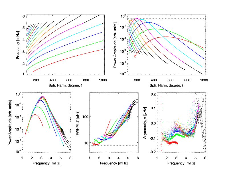
Figure 2: Results from ridge fitting, namely ridge frequency, amplitude, FWHM and asymmetry, once reduced to multiplets. Top left panel: coverage of the fitting in the $\ell-\nu$ plane. The color corresponds to the value of the order, $n$, while the black dots are the a posteriori rejected values, corresponding to the largest order for each degree (see text for explanation). The same color scheme is used in all the panels. Top right panel: power amplitude as a function of degree, the two horizontal lines are in the 1:500 ratio. Lower left panel: power amplitude as a function of frequency. Lower middle panel: FWHM as a function of frequency, the horizontal dash line corresponds to $W_{N,T}$, the spectral resolution of the $N$th order sine multi-taper ($N=61$ and $T=90$ days). Lower right panel: asymmetry as a function of frequency. Notice how the FWHM and asymmetry of the rejected values (black dots) are indeed suspicious.

We should point out that the reduction from singlets to multiplets consists not only of fitting Clebsch-Gordan coefficients to the frequencies, but also of fitting polynomials in $m/\ell$ for the amplitude, FWHM and asymmetry. This is explained and justified in the next sections.

3.1 The Ridge to Mode Correction Methodology

The methodology we implemented to recover mode characteristics from ridge fitting consists of modeling in detail the contribution of all the modes to a given ridge. This model is used to generate a synthetic spectrum that is fitted in a way similar to the data, and produces a correspondence between ridge characteristics and mode characteristics. This method, initially presented in Korzennik et al. (2004), was further expanded, fine tuned and refined as described in Rabello-Soares et al. (2008a).

More recently, we revisited the methodology to not only recover the mode frequency, but also the FWHM, asymmetry and amplitude. The codes for the modeling and for the fitting were converted from a 4GL programming language (IDL) to a compiled language (F90) to make efficient use of the Smithsonian Institution High Performance Computing cluster, a machine with, to date, a little over 2,600 compute cores. In the process, the modeling code was also restructured so as to clearly identify all the input parameters used by the methodology.

3.1.1 The Modeling Methodology

The modeling method consists of producing synthetic spectra by overlapping all the individual modes that leak into a simulated snippet of spectrum around a given mode. Thus for each $\{n,\ell,m\}$, the model consists in computing the power spectrum estimated for a limited frequency range, $w$, centered on $\nu_{n,\ell,m}$, and given by the following superposition:

$$P_{\ell,m}(\nu)=\left(\sum_{\ell^{\prime}}\sum_{m^{\prime}}Q_{\ell^{\prime},m^{\prime}}^{n,\ell,m}{\cal L}_{a}(\nu,\nu_{n,\ell^{\prime},m^{\prime}},\Gamma_{n,\ell^{\prime}},\alpha_{n,\ell^{\prime}})\right)\otimes{\cal X}(\nu,N,W_{T})+B_{p}^{\ell,m}$$ (5)

where $\otimes$ is the convolution operator, ${\cal X}(\nu,N,W_{T})$ is an empirically derived function, $N$ the number of sine multi-tapers, $W_{T}=1/T$ the spectral resolution corresponding to a time series of length $T$, and $B_{p}$ represents the power background value. The frequency range of the model, $w$, is given by

$$w=15\,(\Gamma_{n,\ell}+\frac{\partial\nu}{\partial\ell})$$ (6)

as to cover the full extent of the ridge. The empirical convolution function, $\cal X$, is given by:

$${\cal X}(\nu,N,W_{T})=\left\{\begin{array}[]{ll}(1-(\frac{2\,\nu}{W_{N,T}\,f_{N}})^{2})^{\frac{1}{N}}&\mbox{if $|\nu|\leq\frac{W_{N,T}\,f_{N}}{2}$}\\ 0&\mbox{otherwise}\\ \end{array}\right.$$ (7)

where $f_{N}$ is the factor needed to keep the FWHM of $\cal X$ to remain equal to $W_{N,T}=N\,W_{T}$, the resolution of the $N$th order sine multi-taper. Note that the FWHM of the convolution ${\cal L}\otimes{\cal X}$, the effective FWHM, $\Gamma^{E}_{n,\ell}$, is

$$\Gamma^{E}_{n,\ell}=\sqrt{\Gamma^{2}_{n,\ell}+W_{N,T}^{2}}$$ (8)

i.e., the mode FWHM widened, in quadrature, by the resolution of the $N$th order sine multi-taper. For cases where $\Gamma_{n,\ell}>W_{N,T}$, the result of the convolution is nearly equivalent to an asymmetric Lorentzian with that effective FWHM. But for cases where $\Gamma_{n,\ell}<W_{N,T}$ (narrow modes, the low $\ell$ and low $n$ cases) the shape of ${\cal L}\otimes{\cal X}$ is no longer an asymmetric Lorentzian, as illustrated in Fig. 3. As a result, the ridge produced by the superposition described by Eq. 5, for intrinsically narrow modes, is narrower than the result of superposing widened Lorentzians.

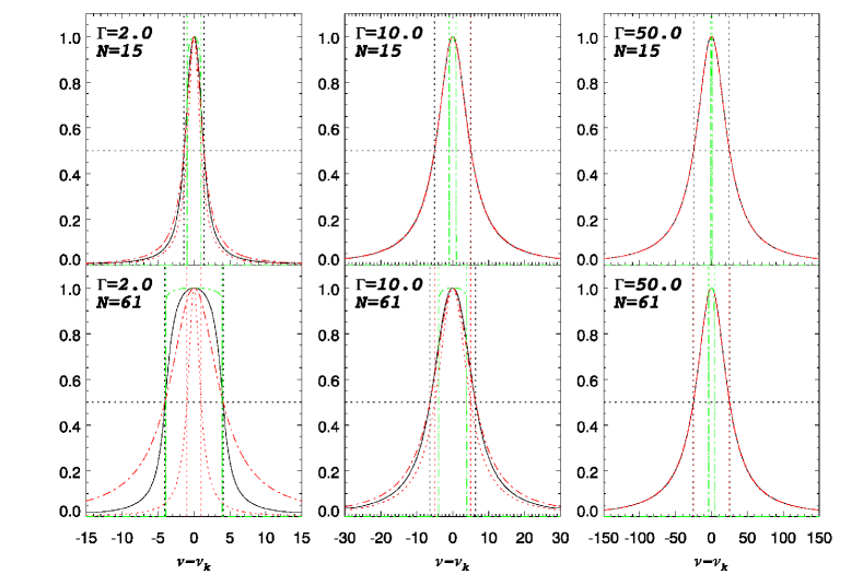
Figure 3: Example of convolutions ${\cal L}\otimes{\cal X}$ (see text), for two values of $N$ (top and bottom panels) and three values of $\Gamma$ (left to right). The black curves are the resulting convolutions, the dash red and green curves represent ${\cal L}$ and ${\cal X}$, respectively, while the red dot-dash curves correspond to the widened ${\cal L}$, using the effective FWHM. The vertical lines indicate the corresponding FWHM. Only for the large $N$ and narrow peak example does the resulting convolution differ substantially from a widened Lorentzian. This corresponds to the modeling of low $\ell$ low $n$ ridges.

The mode profiles are represented by asymmetric Lorentzians, ${\cal L}_{a}$, as defined in Eq. 2 while the frequencies, $\nu_{n,\ell,m}$ and $\nu_{n,\ell^{\prime},m^{\prime}}$, are estimated using

$$\nu_{n,\ell,m}=\nu_{n,\ell,m=0}+\delta\nu_{n,\ell}(m)$$ (9)

and

$$\nu_{n,\ell^{\prime},m^{\prime}}=\nu_{n,\ell^{\prime},m=0}+\delta\nu_{n,\ell^{\prime}}(m^{\prime})$$ (10)

and where

$$\delta\nu_{n,\ell}(m)=\sum_{i=1}^{6}a_{i}(n,\ell)P_{i}(\frac{m}{L})$$ (11)

The amplitude of the leaked power, $Q$, is given by:

$$Q_{\ell^{\prime},m^{\prime}}^{n,\ell,m}=(\tilde{C}_{\ell^{\prime},m^{\prime}}^{n,\ell,m})^{2}R_{p}(\ell,\ell^{\prime})$$ (12)

where $\tilde{C}$ corresponds to the distorted spatial leak coefficients, the sum of the radial and horizontal components:

$$\tilde{C}_{\ell^{\prime},m^{\prime}}^{n,\ell,m}=\tilde{C}_{r}(\ell^{\prime},m^{\prime};\ell,m)+\beta_{n,\ell}\,\tilde{C}_{h}(\ell^{\prime},m^{\prime};\ell,m)$$ (13)

with $\beta_{n,\ell}$ being the ratio of the horizontal to the vertical displacement components.

The power ratio term, $R_{p}$, is introduced to represent the power attenuation with degree resulting from the instrumental PSF, and is parametrized by a polynomial expansion as follows:

$$\log\left[R(\ell,\ell^{\prime})\right]=\sum_{k=0}^{2}c^{R}_{k}(\ell)\,(\ell^{\prime}-\ell)^{k}$$ (14)

The distortion of the leaks by the differential rotation is given by

$$\tilde{C}_{x}(\ell^{\prime},m^{\prime};\ell,m)=\sum_{\ell^{\prime\prime}}G^{\ell^{\prime\prime}}_{\ell^{\prime},m^{\prime}}C_{x}(\ell^{\prime\prime},m^{\prime};\ell,m)$$ (15)

for $x=r,h$, i.e., the radial and horizontal components, respectively. The mixing coefficients, $G$, derived by Woodard (1989), are:

$$G^{\ell^{\prime}}_{\ell,m}=G^{\ell^{\prime}}_{\ell,m}(b_{2},b_{4},\frac{\partial\nu}{\partial\ell})=(-)^{p}\int_{-\pi}^{\pi}\cos(p\Theta+\delta\Phi(\Theta))d\Theta$$ (16)

where

$$p = \frac{\ell-\ell^{\prime}}{2}$$ (17)

$$\delta\Phi(\Theta) = c_{0}(c_{1}\sin(\Theta)+c_{2}\sin(2\Theta))$$ (18)

$$c_{0} = -\frac{m}{2}\,\frac{1}{\frac{\partial\nu}{\partial\ell}}$$ (19)

$$c_{1} = -\frac{1}{2}(b_{2}\,y^{2}+b_{4}\,y^{4})$$ (20)

$$c_{2} = \frac{1}{16}b_{4}\,y^{4}$$ (21)

$$y^{2} = {1-(\frac{m}{L})^{2}}$$ (22)

and where $b_{2}$ and $b_{4}$ represent the solar differential rotation, when parametrized as

$$\frac{\Omega(\theta)}{2\pi}=b_{0}+b_{2}\cos^{2}\theta+b_{4}\cos^{4}\theta$$ (23)

with $\theta$ being the co-latitude and $\Omega(\theta)$ the surface rotation rate.

The undistorted leakage coefficients, $C$, are given by the following integrals (see Korzennik et al., 2004):

$$C_{r}({\ell,m;\ell^{\prime},m^{\prime}}) = \hskip 11.49995pt\oint WY^{m{\ast}}_{\ell}Y^{m^{\prime}}_{\ell^{\prime}}\sin\theta\cos\phi\,d\Omega$$ (24)

$$C_{\theta}({\ell,m;\ell^{\prime},m^{\prime}}) = \!\!\!\!-\frac{1}{L}\oint WY^{m{\ast}}_{\ell}\partial_{\theta}Y^{m^{\prime}}_{\ell^{\prime}}\cos\theta\cos\phi\,d\Omega$$ (25)

$$C_{\phi}({\ell,m;\ell^{\prime},m^{\prime}}) = \frac{1}{L}\oint WY^{m{\ast}}_{\ell}\partial_{\phi}Y^{m^{\prime}}_{\ell^{\prime}}\frac{1}{\sin\theta}\sin\phi\,d\Omega$$ (26)

where ^∗ represents the complex conjugate operator, $Y^{m}_{\ell}$ the spherical harmonic of degree $\ell$ and azimuthal order $m$, $\theta$ and $\phi$ the co-latitude and longitude respectively, and $W(\theta,\phi)$ the spatial window function of the observations – i.e., the function that delimits the angular span of the observations and that includes any additional attenuation like the spatial apodization. The two components of the leakage matrix are the radial component $C_{r}$ and the horizontal components $C_{h}=C_{\theta}+C_{\phi}$. The complete list of the input parameters for our modeling is summarized in Table 2.

$\nu_{n,\ell}$	mode frequency
$\Gamma_{n,\ell}$	mode FWHM
$\alpha_{n,\ell}$	mode asymmetry
$B_{p}(\ell)$	power background
$a_{i}(n,\ell)$	frequency splittings coefficients
$c^{R}_{k}(\ell)$	coefficients defining the power ratio wrt $\ell$
$b_{2},b_{4}$	parametrization of the surface differential rotation
$N_{\delta\ell^{\prime}},N_{\delta m^{\prime}}$	extent of sum on $\ell^{\prime}$ and $m^{\prime}$ in Eq. 5
$N_{\delta\ell^{\prime\prime}}$	extent of sum on $\ell^{\prime\prime}$ in Eq. 15
$C_{r},C_{h}$	radial and horizontal leakage matrix coefficients
$\beta_{n,\ell}$	horizontal to vertical ratio, $\beta_{n,\ell}=(\frac{\nu_{n,\ell}}{\nu_{0,\ell}})^{2}$
$\frac{\partial\nu}{\partial\ell}$	tabulated values, derived from $\{\nu_{n,\ell}\}$

Table 2: List of input parameters, and secondary input parameters (bottom, whose values are derived from the primary parameters), for the ridge modeling.

3.1.2 Model Derivation

A model was run at first using some initial input parameters. We ran it for every degree between $\ell=100$ and $\ell=1000$, and for 51 values of $m$, spanning uniformly the $[-\ell,+\ell]$ interval. That initial input set was derived using results from ridge fitting as well as results from mode fitting at low and intermediate degrees, namely:

• The values for the mode frequencies, $\nu_{n,\ell}$, were derived from ridge fitting results, after smoothing them using a bivariate polynomial in $n$ and $\ell$.

• The FWHM values, $\Gamma_{n,\ell}$, were derived from values obtained by fitting individual modes at low and intermediate degrees combined with values derived from ridge fitting, corrected in a somewhat crude way for the mode to ridge widening.

• The asymmetry, $\alpha_{n,\ell}$, was set to be a bivariate polynomial in $\nu$ and $\ell$, based on ridge fitting results (since, as shown below, the ridge asymmetry is a good estimate of the mode asymmetry).

• The background values, $B_{p}(\ell)$, were set by a polynomial in $\ell$, derived from the fit to the zonal power spectra.

• The frequency splitting coefficients, $a_{i}(n,\ell)$, were determined from a polynomial in $\log(\nu/L)$, with only even non-zero coefficients. These coefficients were derived by fitting low and intermediate frequency splittings, estimated by fitting resolved modes.

• The power ratio coefficients, $c^{R}_{k}(\ell)$, were derived by fitting $\frac{\partial\log\tilde{A}}{\partial\ell}$, where the power amplitudes, $\tilde{A}$, correspond to measured zonal ridge power amplitudes, themselves smoothed using a bivariate polynomial in $\nu$ and $\ell$.

• The ratio $\beta_{n,\ell}$ was set to $(\nu_{n,\ell}/\nu_{n=0,\ell})^{2}$, after fitting a cubic polynomial in $\sqrt{L}$ to the f-mode frequencies derived from ridge fitting.

• We adopted $b_{2}=-69.6\pm 1.7$ nHz and $b_{4}=-58.8\pm 2.9$ nHz, values derived from a rotation inversion of a co-eval epoch using individual resolved modes at low and intermediate degrees (Eff-Darwich & Korzennik, 2012).

• The derivative $\frac{\partial\nu}{\partial\ell}$ was computed directly from the set of $\{\nu_{n,\ell}\}$.

• The extent of the summations were set to

  $$N_{\delta\ell^{\prime}}=\left\{\begin{array}[]{ll}10&\ell\leq 400\\ 2(1+\ell/100)&\mbox{otherwise}\end{array}\right.$$ (27)

  $$N_{\delta\ell^{\prime\prime}}=\left\{\begin{array}[]{ll}12&\ell\leq 600\\ 2\ell/100&\mbox{otherwise}\end{array}\right.$$ (28)

  while $N_{\delta m}=10$. These values were determined to be optimum in Rabello-Soares et al. (2008a).

• The coefficients of the leakage matrix, $C_{r},C_{h}$, were computed by one of us (JS) to correspond to the spatial decomposition of the MDI Dynamics observations.

Figures 4 to 6 present the key properties of this model. Figure 4 shows the raw frequency offset (i.e., the difference between the target mode and the ridge frequency), while Fig. 5 shows on the one hand the zonal frequency offset, $\Delta^{\nu}_{n,\ell,m=0}$, and how it scales primarily with frequency, and on the other, the frequency offset with respect to its corresponding zonal value, $\Delta^{\nu}_{n,\ell,m}-\Delta^{\nu}_{n,\ell,m=0}$ divided by the $\ell$, since this quantity scales linearly with $\ell$. Once scaled, it is mostly a function of the relative azimuthal order, $\frac{m}{\ell}$.

Figure 6 shows the mode to ridge widening, for the zonal ridges, and also how the ridge width varies with the relative azimuthal order, $\frac{m}{\ell}$, even though the mode width itself, an input parameter to the model, is constant with $m$. Similarly, that figure shows that the ridge asymmetry changes with $\frac{m}{\ell}$, while the corresponding input model mode asymmetry is also constant with $m$. The distortion of the eigenvalues by the differential rotation changes the observed power distribution with a strong dependence on $m$ – hence it not only changes the ridge central frequency but its width and asymmetry.

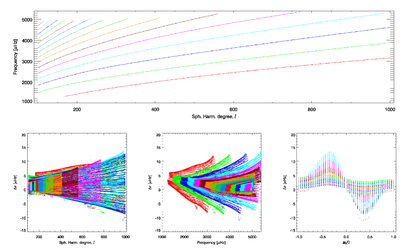
Figure 4: Top panel: coverage in the $\ell-\nu$ of the modeling (shown for $m=0$ only), the color corresponds to different values of $n$. Bottom panels: frequency offsets, $\Delta^{\nu}$, between mode and ridge frequency as a function of degree, $\ell$ (left), frequency, $\nu$ (middle), and relative azimuthal order, $m/\ell$ (right).

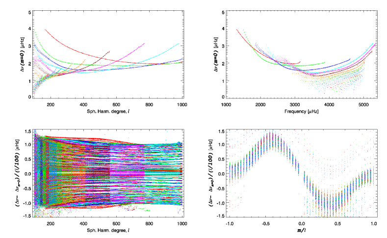
Figure 5: Top panels: frequency offsets, $\Delta^{\nu}$, between mode and ridge frequency (as in Fig. 4) but for $m=0$ only, plotted as a function of degree or frequency. Bottom panels: frequency offsets with respect to the corresponding zonal value and divided by $\ell/100$, also plotted versus degree or frequency. Note how $\Delta^{\nu}_{m=0}$ is primarily a function of $\nu$, while $(\Delta^{\nu}-\Delta^{\nu}_{m=0})/\ell$ is primarily a function of $m/\ell$. The color corresponds to the value of the order, $n$.

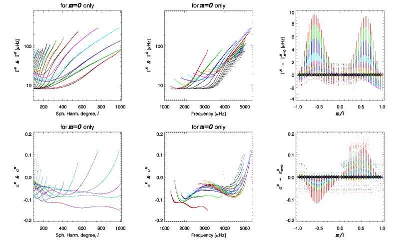
Figure 6: Top panels: comparison of the model’s ridge FWHM (colored dots) to the input effective FWHM (black dots), versus degree, frequency or $m/\ell$ (left to right respectively). Bottom panels: comparison of the model’s ridge asymmetry (colored dots) to the input asymmetry (black dots), versus degree, frequency or $m/\ell$ (left to right respectively). The left two panels in both rows show only the $m=0$ values. The right most panels show the variation with respect to the corresponding zonal values as a function of the relative azimuthal order. The diamond symbols in these panels correspond to the model mode input values: both $\Gamma^{E}_{n,\ell}$ and $\alpha_{n,\ell}$ are constant with $m$. The variation seen here results primarily from the variation of the leakage with $m$. The color corresponds to the value of the order, $n$.

3.1.3 The Modeling Iterative Process

Some of the input parameters are not precisely known a priori since they are the parameters we want to estimate accurately, and are thus approximated by values derived from ridge fitting. While we have shown that the ridge to mode frequency correction sensitivity to these input parameters is small (Rabello-Soares et al., 2008a), we recognize that improving the input parameters whenever possible can only improve the accuracy of such corrections. In our continuing effort to improve our determination of unbiased mode parameters at high-degrees, we implemented an iterative procedure to adjust some of the input parameters so as to produce a ridge model whose characteristics match the measured ridge values.

We adjusted iteratively the following parameters of the model input set: $\nu_{n,\ell}$, $\Gamma_{n,\ell}$, $\alpha_{n,\ell}$, $a_{i}({n,\ell})$ and $c_{k}^{R}(\ell)$. It consisted of the following adjustments at each iteration step:

• Input frequencies, $\nu_{n,\ell}$:

  $$\nu_{n,\ell}\leftarrow\nu_{n,\ell,m}\leftarrow\tilde{\nu}_{n,\ell,m}-\Delta^{\nu}_{n,\ell,m}$$ (29)

  where $\tilde{\nu}$ is the observed ridge frequency, estimated by fitting the observations, and $\Delta^{\nu}_{n,\ell,m}$ is the ridge to mode frequency offset predicted by the model –i.e., the model resulting ridge frequency minus the model input mode frequency– interpolated at each $m$, using a polynomial fit in $\frac{m}{\ell}$. The singlets frequencies, $\nu_{n,\ell,m}$, are then reduced to multiplets, $\nu_{n,\ell}$, by fitting Clebsch-Gordan coefficients.

• The FWHM, $\Gamma_{n,\ell}$, is adjusted at each iteration as follows:

  $$\Gamma_{n,\ell}\leftarrow\sqrt{(\tilde{\Gamma}^{M}_{n,\ell}\,f^{\Gamma}_{n,\ell})^{2}-W_{N,T}^{2}}$$ (30)

  where the factor $f^{\Gamma}$ is given by

  $$f^{\Gamma}_{n,\ell}=<\tilde{\Gamma}_{n,\ell,m}/\tilde{\Gamma}_{n,\ell,m}^{M}>$$ (31)

  and $\tilde{\Gamma}_{n,\ell,m}$ is the ridge FWHM estimated by fitting the observations, while $\tilde{\Gamma}_{n,\ell,m}^{M}$ is the ridge FWHM measured when fitting the model, interpolated at each $m$ by a polynomial fit in $\frac{m}{\ell}$. The brackets represent averaging over $m$. The quantity $W_{N,T}$ is the frequency resolution, set to the resolution of the observations ($N=61$ and $T=90$ days).

• Input asymmetry, $\alpha_{n,\ell}$, similarly is adjusted at each iteration as follows:

  $$\alpha_{n,\ell}\leftarrow\alpha^{M}_{n,\ell}\,f^{\alpha}_{n,\ell}$$ (32)

  where the factor $f^{\alpha}$ is given by

  $$f^{\alpha}_{n,\ell}=<\tilde{\alpha}_{n,\ell,m}/\tilde{\alpha}_{n,\ell,m}^{M}>$$ (33)

  and $\tilde{\alpha}_{n,\ell,m}$ is the ridge asymmetry estimated by fitting the observations, while $\tilde{\alpha}_{n,\ell,m}^{M}$ is the ridge asymmetry measured when fitting the model, interpolated at each $m$ by a polynomial fit in $\frac{m}{\ell}$. The brackets represent averaging over $m$.

• Amplitudes and $c_{k}^{R}(\ell)$ are also re-adjusted at each iteration as follows:

  $$A_{n,\ell}\leftarrow A^{M}_{n,\ell}/(\sum_{k}f^{A}_{k}\ell^{k})$$ (34)

  where the polynomial $\sum_{k}f^{A}_{k}\ell^{k}$ is determined by fitting the ratio $\tilde{A}^{M}_{n,\ell,m=0}/\tilde{A}_{n,\ell,m=0}$ with respect to $\ell$. $\tilde{A}^{M}$ and $\tilde{A}$ represent the model and the observed ridge power amplitudes, respectively, for the zonal modes.

  The $c_{k}^{R}(\ell)$ coefficients are then derived by fitting $\frac{\partial\log A}{\partial\ell}$.

• The following input variables are then readjusted or, for the secondary input parameters, recomputed as follows:

  • The FWHM, $\Gamma_{n,\ell}$, and the asymmetry, $\alpha_{n,\ell}$, are smoothed using a bivariate polynomial in $\nu$ and $\ell$.

  • The splittings coefficients, $a_{i}(n,\ell)$, are recomputed using the new input frequencies.

  • The horizontal to vertical ratio, $\beta$, is recomputed using the same prescription as in the preceding section, but using the new input frequencies.

  • The derivative, $\frac{\partial\nu}{\partial\ell}$ is recomputed using the new input frequencies.

This procedure was run for some 10 iterations, where the models were computed only every 5th degree. The resulting input set was then used to compute a final model at each degree. After a handful of iterations, the characteristics of the model barely changed and the procedure converged, with relative changes at the last steps of the iterative process at the 0.1% level.

3.1.4 Sensitivity of the Model

The values for $\nu_{n,\ell}$, $\Gamma_{n,\ell}$, $\alpha_{n,\ell}$, $c^{R}_{k}$ and $a_{i}({n,\ell})$ have been fine tuned using an iterative process. Since the resulting ridge model values when using these parameters match the observed ridge values, their uncertainty and thus the corresponding model sensitivity can be estimated by the changes at the last iteration (0.1%). A more conservative alternative approach is to perturb each value by its corresponding measured ridge uncertainty.

We computed additional models where some input parameters were increased by their corresponding observational uncertainty.

The effect of perturbing the modes amplitudes, $A$, frequencies, $\nu$, FWHM, $\Gamma$, asymmetry, $\alpha$, and, rotational splittings, $a_{i}$, by one-sigma are illustrated in Fig. 7, where the relative change of the frequency offsets between ridge and mode, $\Delta^{\nu}$, is shown as the change of the zonal offset, $\Delta^{\nu}_{n,\ell,m=0}$, and as the change of the scaled frequency offset with respect to the zonal value, $(\Delta^{\nu}_{n,\ell,m}-\Delta^{\nu}_{n,\ell,m=0})/\ell$. Note how the zonal offset is barely affected, except when perturbing the FWHM. The azimuthal signature is also small with just the FWHM perturbation showing a systematic and specific change.

The input parameters $\beta_{n,\ell}$, the horizontal to vertical ratio, $b_{2},b_{4}$, the coefficients corresponding to the parametrization of the surface differential rotation, and $C_{r},C_{h}$, the leakage matrix coefficients, were not iterated upon. The sensitivity of the model to their accuracy needs also to be estimated.

The value of $\beta_{n,\ell}$ is well constrained by the values of $\nu_{n,\ell}$ under the prescription we used. Still, this prescription does not force $\beta_{n=0,\ell}$ to be exactly unity. This prescription is also based on estimating that ratio using a formula resulting from a specific outer boundary condition, namely that the Lagrangian pressure perturbation vanish ($\delta p=0$), in the small amplitude oscillation equations for the adiabatic and non-magnetic case. While this is most likely a very good approximation, the conditions near the surface are not adiabatic, and the ratio $\beta$ might not be exactly the one predicted by the adiabatic case. Rhodes et al. (2001) estimated that $\beta$ is $0.995\pm 0.004$ of the theoretical value. We ran models with perturbed values of $\beta$ to assess their sensitivity to this parameter. The effect of perturbing $\beta$ is illustrated in Fig. 8. That figure shows that the zonal frequency offset changes proportionally to the perturbation, while the change of the scaled offset with respect to the zonal values displays a small azimuthal signature that peaks at the 1 and 2% levels, respectively (in terms of relative change of the offset).

We selected our best estimate for $b_{2}=-69.6\pm 1.7,b_{4}=-58.8\pm 2.9$ nHz, using our own inversion profile derived from measuring rotational frequency splittings at low and intermediate modes for a co-eval epoch (Eff-Darwich & Korzennik, 2012). We have computed models using one-sigma perturbation in $b_{2}$ and $b_{4}$, as shown in Fig. 9, to assess the effect of perturbing the parametrization of the surface differential rotation used to compute the mode mixing resulting from the distortion of the eigenfunctions by the differential rotation. The change of the zonal frequency offset is negligible (at the 0.1% level), while the change of the scaled offset with respect to the zonal values displays a clear azimuthal signature at the 2% level. This illustrates the interdependency between knowing the rotation profile to properly correct the frequency splittings and deriving the rotation profile from the splittings.

Finally, to quantify the sensitivity of our result to the leakage matrix coefficients, we computed models that use an independent estimate of the leakage coded by one of us (SK). The leakage was computed by spatially decomposing images of the three components of the line of sight velocity signal (see Eqs. 24 to 26). The sampling of these images and their spatial apodization were set so as to correspond to the MDI Dynamics observations. This was carried out for the same subset of $(\ell,m)$, as for the reference leakage matrix coefficients (computed by JS).

We computed a set of leakage matrix coefficients for $B_{o}=0$, where $B_{o}$ is the heliographic latitude at disk center, and for $B_{o}=-5.68^{\rm o}$, the mean value of $B_{o}$ for the 2001 Dynamics epoch. We computed another set for that same value of $B_{o}$, but including an estimate of the PSF of MDI. That estimate was derived from running the procedure HGEOM, a procedure that is part of the GONG reduction and analysis software package. HGEOM returns an estimate of the azimuthaly averaged MTF (i.e., the Fourier transform of the PSF, see Korzennik et al., 2004, and references therein). We thus also included an axisymmetric PSF, whose profile was set by the MTF estimated by HGEOM.

The changes resulting from using different leakage matrices are presented in Fig. 10. This figure shows that using a different leakage matrix computation produces a relative change in the zonal frequency offset at the 1% level, except when including a PSF, where that change peaks at 5%. Similarly, the largest change in the scaled offset with respect to the zonal offset is seen when including a PSF. These results corroborate our previous conclusions (Korzennik et al., 2004) that the largest contribution to the uncertainty of the high degree mode properties is our limited knowledge of the PSF of the MDI instrument.

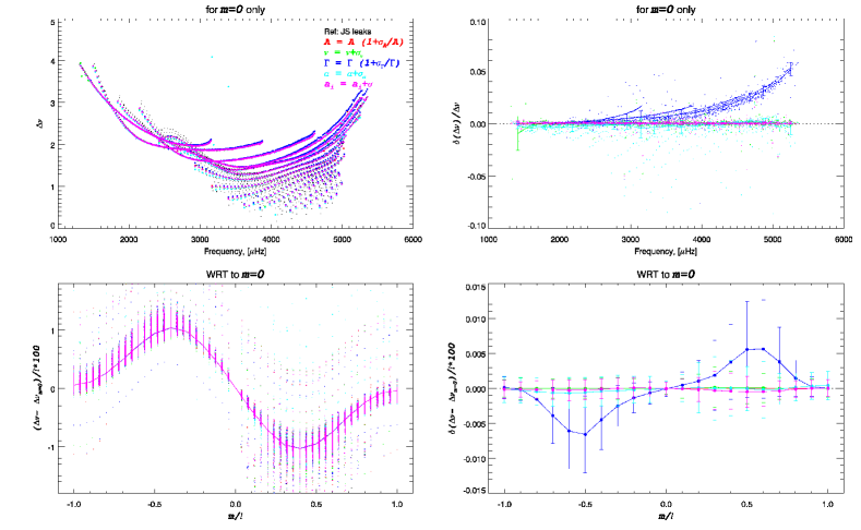
Figure 7: Comparison of the ridge to mode frequency offset, produced by different models. The top panels show the zonal modes only as a function of frequency, while the bottom panels show the scaled offset, relative to the zonal values, as a function of $m/\ell$. The left panels compare the offset, the right panels show the relative difference (top right) or the difference (bottom right). The lines with error bars represent binned values and the scatter within each bin. The models correspond to perturbing the modes amplitudes, $A$, frequencies, $\nu$, FWHM, $\Gamma$, asymmetry, $\alpha$, and, rotational splittings, $a_{i}$, by one-sigma.

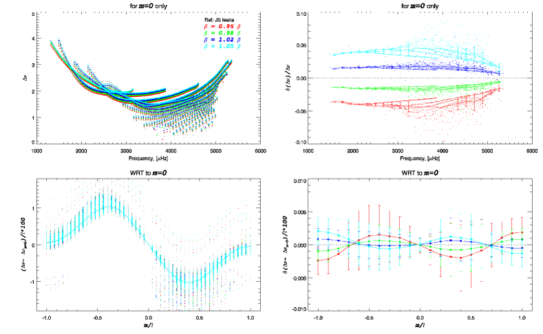
Figure 8: Comparison of the ridge to mode frequency offset, produced by different models, in the same format as Fig. 7. The effect of perturbing the horizontal to vertical ratio, $\beta$, is illustrated for positive and negative perturbation of 2 and 5%.

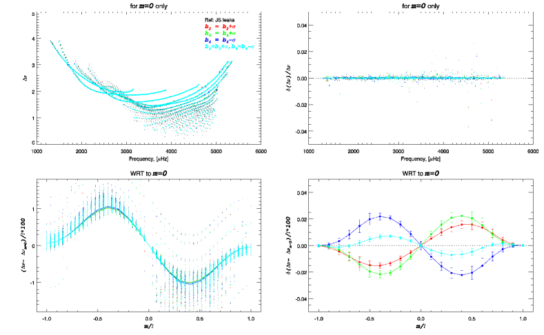
Figure 9: Comparison of the ridge to mode frequency offset, produced by different models, in the same format as Figs. 7 and 8. The figures show the effect of perturbing the parametrization of the surface differential rotation ($b_{2},b_{4}$) used to compute the mode mixing resulting from the distortion of the eigenfunctions by the differential rotation.

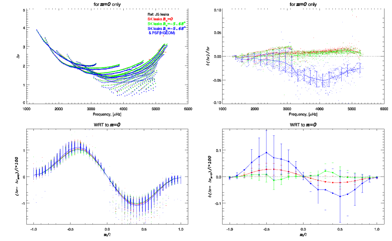
Figure 10: Comparison of the ridge to mode frequency offset, produced by different models, in the same format as Figs. 7 to 9. The effect of using different leakage matrix coefficients (see text for description) is illustrated, using two different and independent implementations (black versus colors), including the actual mean value of $B_{o}$ (in red and green), as well as including an axisymmetric instrumental PSF (in blue).

		Frequency offset relative sensitivity
Parameter	Perturbation	zonal	azimuthal
frequency, $\nu$	$1\ \sigma$	$0.001\pm 0.002$ (0.009)	0.001 ($0.001\pm 0.002$)
FWHM, $\Gamma$	$1\ \epsilon$	$0.012\pm 0.012$ (0.052)	0.007 ($0.001\pm 0.005$)
asymmetry, $\alpha$	$1\ \sigma$	$0.003\pm 0.006$ (0.004)	0.001 ($0.001\pm 0.002$)
amplitude, $A$	$1\ \epsilon$	$0.001\pm 0.001$ (0.001)	0.001 ($0.001\pm 0.001$)
splittings, $a_{i}$	$1\ \sigma$	$0.001\pm 0.001$ (0.001)	0.001 ($0.001\pm 0.002$)
ratio, $\beta$	2%	$0.016\pm 0.005$ (0.018)	0.001 ($0.001\pm 0.002$)
rot.  $b_{2},b_{4}$	$1\ \sigma$	$0.001\pm 0.001$ (0.001)	0.022 ($0.001\pm 0.014$)
leakage matrix	$B_{o}=0^{\rm o}$	$0.008\pm 0.006$ (0.013)	0.028 ($0.001\pm 0.023$)
leakage matrix	$B_{o}=-5.68^{\rm o}$	$0.005\pm 0.008$ (0.011)	0.021 ($0.001\pm 0.020$)
leakage matrix	$B_{o}=-5.68^{\rm o}$ & PSF	$-0.029\pm 0.022$ (0.051)	0.091 ($0.004\pm 0.076$)

Table 3: Sensitivity of the ridge to mode frequency offset with respect to the model’s input parameters. The zonal values are characterized by the mean and RMS of the differences (and within parenthesis the maximum of the absolute value of the binned differences), while the azimuthal values are characterized by the maximum of the absolute value of the binned differences (and within parenthesis the mean and RMS of the raw differences).

The relative change of $\Delta^{\nu}$ for all the perturbed models, presented in Figs. 7 to 10, are also summarized in Table 3, where the zonal values are characterized by the mean and RMS of the differences, while the azimuthal values are characterized by the maximum of the absolute value of the binned differences.

The sensitivity of the ridge to mode frequency offset to a $1\,\sigma$ perturbation is indeed at the 0.1% level, but for the FWHM and for changes of $\beta$ and the leakage matrix. In the case of the FWHM, the $1\,\sigma$ perturbation is a large perturbation because the ridge fitting precision is low. Such a perturbation produces a model whose ridge width is, on average, off by 4% (versus 0.2% for the reference model) when compared to the observed ridge width. So the model precision is constrained by producing a model that matches the observations and not by the uncertainty on the ridge width. As for the sensitivity with $\beta$ we see that it is proportional to the perturbation, so if we consider that $\beta$ may be off by as much as 0.5% from the theoretical value (Rhodes et al., 2001), the model uncertainty is at most at the 0.4% level. As for the sensitivity of our model to a particular leakage matrix, we see large changes associated to our limited knowledge of the PSF of the MDI instrument. A more conservative estimate of the model precision is thus more at the 0.5% level than the 0.1% level, but could be as large as a few percent if the leakage matrix we use is off. We opted, somewhat arbitrarily, to use 0.1% and 1% as basic and conservative values for the precision of $\Delta^{\nu}$, the ridge to mode frequency offset.

4 Results

The approach we used to derive the characteristics of high degree modes is to fit and characterize the power ridges and compute a sophisticated model of the ridge power to estimate the bias between the ridge characteristics and the underlying characteristics of the mode. While the most useful and sought after characteristic is the mode frequency, we have also expanded our efforts to derive estimates of the mode width, its asymmetry and its amplitude.

4.1 Frequencies & Frequency Splittings

Mode blending causes the ridge frequency to be offset with respect to the underlying target mode frequency. Our ridge model allows us to estimate this offset, and the sensitivity of that estimate on the model input parameters. We have thus computed this offset for every degree between $\ell=100$ and $\ell=1000$, and each order for which the ridge was fitted, but only for 51 values of $m$ spanning the $[-\ell,+\ell]$ range. We used a polynomial fit in $m/\ell$ to re-sample the offset at each $m$.

An estimate of the mode frequency is computed by subtracting from the measured ridge frequency the ridge to mode frequency offset:

$$\nu_{n,\ell,m}=\tilde{\nu}_{n,\ell,m}-\Delta^{\nu}_{n,\ell,m}$$ (35)

where $\tilde{\nu}$ is the ridge frequency and $\Delta^{\nu}$ the ridge to mode offset:

$$\Delta^{\nu}_{n,\ell,m}=\tilde{\nu}^{M}_{n,\ell,m}-{\nu}^{M}_{n,\ell,m}$$ (36)

${\nu}^{M}$ being the mode frequency and $\tilde{\nu}^{M}$ the resulting ridge frequency in our model. The frequency multiplets, $\nu_{n,\ell,m}$, are then reduced to singlets, $\nu_{n,\ell}$, by performing the usual Clebsch-Gordan coefficients expansion in $m$.

The uncertainty on the resulting mode frequency estimate is determined by the uncertainty on the ridge estimate and the uncertainty on the correction, the latter being either the precision of the iterative process (0.1%) or a more conservative estimate, as discussed in the previous section (1%). These two uncertainties are presumed independent and therefore combined in quadrature, i.e.:

$$\sigma^{2}_{\nu_{n,\ell,m}}=\tilde{\sigma}^{2}_{\nu_{n,\ell,m}}+\sigma^{2}_{\Delta^{\nu}_{n,\ell,m}}$$ (37)

As described in Sec. 2.1, we have some overlap between mode and ridge fitting covering $100\leq\ell\leq 300$ for f-modes and $100\leq\ell\leq 200$ for p-modes. Figure 11 shows how well the estimate of the mode multiplet frequencies derived from ridge fitting match the actual mode frequency computed by fitting resolved modes. The residual bias is nearly uniform, about 0.3 $\mu$Hz  or at the $1.67\,\sigma$ level. Figure 12 compares the mode singlet frequencies, derived from ridge fitting, to the frequencies computed by fitting resolved modes. The singlets agree at the $0.1\,\sigma$ level, with no trends with degree, frequency of azimuthal order. The scatter of the differences shows some systematic fluctuations with frequency (or order). The distribution of the raw differences, although nearly randomly distributed, show a departure from a Gaussian distribution in the wings (i.e., for the less frequent larger differences), that is asymmetric. This skewness might explain why the comparison of the multiplets shows a larger bias. Note also that the RMS of the scaled differences is 1.4, or a little larger than unity.

Figure 13 shows how well our estimates of the frequency splittings derived from corrected ridge frequencies, once parametrized in terms of Clebsch-Gordan coefficients, match the frequency splittings computed by fitting resolved modes. The substantial offsets present without that correction are canceled by our correction. One is hard-pressed in these plots to see the transition from mode fitting to ridge fitting along a given order.

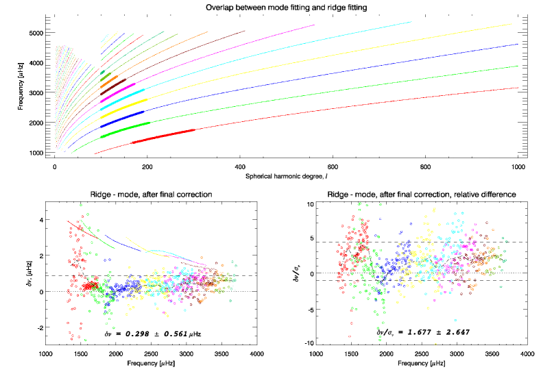
Figure 11: Comparison of estimate of mode multiplet frequencies derived from ridge fitting to actual mode frequency computed by fitting resolved modes at intermediate degrees. The top panel shows the overlap between both methods in the $\ell-\nu$ plane (filled circles). The bottom left panel shows the raw frequency differences (open circles) as a function of frequency, with the dot dash line representing the binned raw differences. The dots on that figure correspond to the ridge to mode frequency correction. The bottom right panel shows the scaled frequency differences, i.e., the frequency differences divided by their respective uncertainties (open circles) as a function of frequency, with the dot dash line representing the binned scaled differences. A dotted line is drawn at 0, while the dotted lines are drawn at the mean and plus or minus one RMS of the raw differences. The color corresponds to the value of the order, $n$.

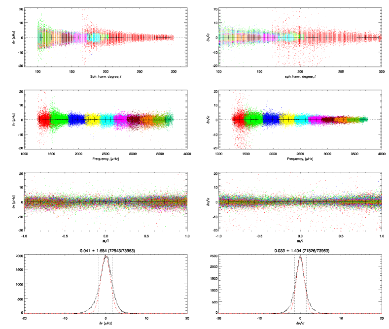
Figure 12: Comparison of estimate of mode singlet frequencies derived from ridge fitting to actual mode frequency computed by fitting resolved modes at intermediate degrees. The frequency differences (left panels), and the scaled differences (differences divided by their respective uncertainties, right panels) are plotted as a function of degree, frequency, and $m/\ell$, and as a histogram (top to bottom). In the top three rows the color corresponds to the value of the degree, $n$, while the black lines represent binned values with the RMS within each bin shown as error bars. These differences show no trend with degree, frequency or relative azimuthal order, but for the scatter. The red curves in the histograms are the Gaussians corresponding to the mean and standard deviation of the distributions (indicated by the vertical dotted lines). Note the excess and skewness in the wings of the actual distribution.

Figure 13: Left panels: comparison of estimates of mode frequencies splittings, parametrized as Clebsch-Gordan coefficients, plotted as a function of the ratio $\nu/L$, a proxy for the mode inner turning point, derived from ridge fitting after correcting for the ridge to mode offset (small dots) to frequency splitting coefficients computed by fitting resolved modes (large dots). The black dots are the frequency splitting coefficients computed from uncorrected ridge frequencies. The corrected splittings match the estimates derived from fitting resolved modes. Right panels: same Clebsch-Gordan coefficients computed by fitting resolved modes, only (same large dots). The color corresponds to the value of the order, $n$. Top to bottom panels correspond to different odd coefficients.

Figure 14 shows how these Clebsch-Gordan coefficients change when correcting the ridge frequencies using mode-to-ridge offsets estimated from models using different leakage matrices. This figure, which presents the same effect than the one presented in Fig. 10, but in terms of splitting coefficients, shows significant changes in the parametrization of the rotational splittings, primarily at the lowest values of $\nu/L$ (shallow modes). As we stated earlier, this results from our limited knowledge of the PSF of the MDI instrument.

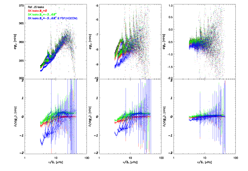
Figure 14: Comparison of estimates of mode frequencies splittings, parametrized as Clebsch-Gordan coefficients, plotted as a function of the ratio $\nu/L$, and derived from ridge fitting after correcting for the ridge to mode offset, using ridge-to-mode offsets computed for the same four different models presented in Fig. 10. The bottom panels show the differences with respect to the reference model, and the coefficients error bars (not shown for each value for clarity). Left to right panels correspond to different odd coefficients. The changes are, for the shallow modes, significantly larger than their uncertainties.

4.2 Widths, Asymmetries & Amplitudes

The most sought after characteristics of solar oscillations are the mode frequencies, since they are the most precise and best understood properties. They have allowed us to infer interesting properties of the Sun. We also realize that the modes FWHM, asymmetry and amplitude are useful properties to characterize, and important quantities when modeling the near surface acoustic field. In a manner similar to the case of the frequencies, the FWHM, amplitude and to a lesser degree the asymmetry estimated by fitting the ridges are not the FWHM, amplitude and asymmetry of the underlying modes. With the assistance of the ridge modeling, we devised specific methodologies to derive estimates of the mode values from the ridge estimates.

4.2.1 FWHM

Figure 15: Top panels: measured ridge FWHM (black dots) as a function of frequency or spherical harmonic degree (left and right panels, respectively), compared to our best model for the ridge FWHM (colored circles), derived from an optimized model for mode FWHM estimates (colored dots), for $m=0$. Note how, for a substantial fraction of modes, the resulting ridge FWHM is much larger than the mode FWHM. The small black dots correspond to cases where the 3-$\sigma$ uncertainty on the ridge width is larger than the mode width estimates. The horizontal line corresponds to $W_{N,T}$, the resolution of the $N$th order sine multi-taper used as spectral estimator. Bottom panels: ratio of model to measured ridge FWHMs, indicating how well our predicted ridge FWHMs agree with the observed ones, but for some residual disagreement at the lowest frequencies, where the mode FWHM is more than an order of magnitude smaller then the resulting ridge FWHM. The different colors correspond to the order, $n$.

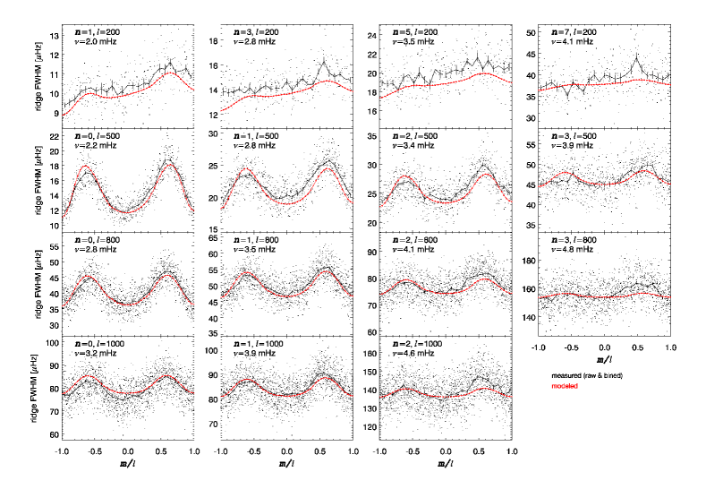
Figure 16: Comparison of ridge FWHM for a selection of multiplets, as a function of the ratio $m/\ell$. The dots correspond to individual ridge width measurements, and the black curves the corresponding binned values. The red curves correspond to our best model of the ridge width, as evaluated at 51 equispaced $m$ values. In most cases, our model reproduces rather well the variation of ridge width with the azimuthal order, $m$, although the input mode width of the model is constant with $m$.

Figure 15 compares the ridge FWHM, $\tilde{\Gamma}$, resulting from ridge fitting to the predicted ridge width from our model, for the zonal modes. The iterative procedure produced a model for the ridge FWHM that matches, but for the very low frequencies, the measured values. The intrinsic mode width estimates used in the model are also shown on that figure. These are, for a substantial fraction of modes, a lot smaller than the ridge widths. In fact, the uncertainty on the fitted ridge width becomes, in some cases, larger than the mode width estimate itself, especially at the low degree end of the low order ridges. For these modes, recovering the intrinsic mode width from ridge fitting is poorly constrained and in some cases too poorly constrained to derive a meaningful estimate.

Figure 16 also compares the measured ridge widths to the model predictions, but as a function of the ratio $m/\ell$, and for a selection of multiplets. This figure illustrates how well our model reproduces the variation of the ridge width with the azimuthal order, although the mode width in the model is constant with $m$.

The zonal ridge FWHM is by no means the mode FWHM. Its value reflects the mode FWHM, the spectral resolution, and as a result of the mode blending, the slope of the ridge with respect to the degree (i.e., $\frac{\partial\nu}{\partial\ell}$), since it is that slope that sets the separation in frequency of the leaks that contribute to the ridge. We devised a simple two step widening model to estimate the mode width from the ridge width. It is based on the Gaussian convolution analogy: the convolution of Gaussian by a Gaussian is also a Gaussian, whose width is the square root of the sum of the square of the convolved Gaussian widths. So by analogy, we relate the width of the ridge to the width of the mode using the following simple and convenient model:

$$\tilde{\Gamma}^{2}_{n,\ell}={(\Gamma^{E}_{n,\ell})}^{2}+{\cal W}_{n,\ell}^{2}$$ (38)

where $\Gamma^{E}_{n,\ell}$ is the effective mode width (as defined in Eq. 8) and ${\cal W}$ is a mode to ridge widening term, that we estimate from our modeling procedure. To account for the ridge fitting uncertainty, we rewrite Eq. 38 as:

$$(\tilde{\Gamma}_{n,\ell}\pm\tilde{\sigma}_{n,\ell})^{2}=(\Gamma^{E}_{n,\ell}\pm\sigma_{n,\ell})^{2}+{\cal W}^{2}_{n,\ell}$$ (39)

The mode to ridge widening term, ${\cal W}$, is estimated from the model

$${\cal W}^{2}_{n,\ell}=(\tilde{\Gamma}^{M}_{n,\ell})^{2}-(\Gamma^{E,M}_{n,\ell})^{2}$$ (40)

where $\Gamma^{E,M}$ is the input model’s effective mode width, i.e., the mode width widened by the spectral resolution, and $\tilde{\Gamma}^{M}$ the model’s resulting ridge width.

This can be rewritten as (after dropping the $n,\ell$ subscripts):

$$\tilde{\Gamma}^{2}+\tilde{\sigma}^{2}+2\,\tilde{\Gamma}\ \tilde{\sigma} = (\Gamma^{E})^{2}+\sigma^{2}+2\,\Gamma^{E}\ \sigma+{\cal W}^{2}$$ (41)

$$\tilde{\Gamma}^{2}+\tilde{\sigma}^{2}-2\,\tilde{\Gamma}\ \tilde{\sigma} = (\Gamma^{E})^{2}+\sigma^{2}-2\,\Gamma^{E}\ \sigma+{\cal W}^{2}$$ (42)

and simple arithmetic leads to the following two equations:

$$\tilde{\Gamma}\ \tilde{\sigma} = \Gamma^{E}\ \sigma$$ (43)

$$\tilde{\Gamma}^{2}+\tilde{\sigma}^{2} = (\Gamma^{E})^{2}+\sigma^{2}+{\cal W}^{2}$$ (44)

from which we derive $\Gamma^{E}$ and $\sigma$ as follows:

$$\sigma = \tilde{\sigma}\frac{\tilde{\Gamma}}{\Gamma^{E}}$$ (45)

$$\Gamma^{E} = \sqrt{\tilde{\Gamma}^{2}-{\cal W}^{2}+g\,\tilde{\sigma}^{2}}$$ (46)

where

$$g=1-(\frac{\tilde{\Gamma}}{\Gamma^{E}})^{2}$$ (47)

This correction factor, $g$, depends on $\Gamma^{E}$ the variable we solve for, but can be re-evaluated iteratively, starting by setting $g=0$, to solve Eq. 46. Only 3 to 4 iterations are needed to reach a $10^{-6}$ precision.

Evaluating of $\Gamma^{E}$ becomes poorly constrained when ${\cal W}^{2}$ is commensurable with $\tilde{\Gamma}^{2}+g\,\tilde{\sigma}^{2}$, since the result of their subtraction must to be a positive quantity. But since $\Gamma^{E}$ must be larger than the spectral resolution, $W_{N,T}$, we can force $\Gamma^{E}$, when derived from Eq. 46, to always be at least $W_{N,T}$.

An estimate of the mode FWHM is then derived from the effective width by solving Eq. 8, hence

$$\Gamma=\sqrt{{\Gamma^{E}}^{2}-W_{N,T}^{2}}$$ (48)

Results of this equation are guaranteed to be greater or equal to zero if $\tilde{\Gamma}^{E}$ is set to always be at least $W_{N,T}$. But estimates of $\Gamma$ much smaller than $W_{N,T}$, derived from $\Gamma^{E}$ according to Eq. 48, are in practice meaningless. To alleviate this, we introduce a reliability threshold, $f_{r}$, as to only infer $\Gamma$ from $\Gamma^{E}$ when $\Gamma\geq W_{N,T}\,f_{r}$. We used $f_{r}=1/4$, namely we derived an estimate of $\Gamma$ using Eq. 48 only when $\Gamma^{E}\geq 1.0308\,W_{N,T}$. This means that for a given $n$ the mode width correction scheme cannot always be extended to the lowest fitted degrees. The results of this correction scheme for the effective width and the mode width are plotted for zonal modes in Fig. 17.

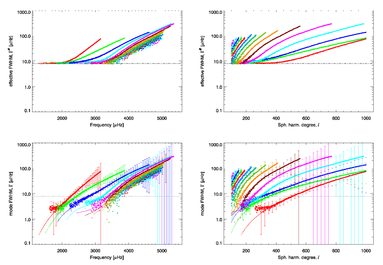
Figure 17: Top panels: effective FWHM, estimated from the ridge width, using the widening model (see description in text), as a function of frequency or degree (left and right panels, respectively). The dots correspond to effective widths below the reliability threshold. Bottom panels: mode FWHM, estimated from the effective width, using a 1/4 threshold (see explanation in text), and their associated uncertainty, as a function of frequency or degree (left and right panels, respectively). The dots in these panels are the mode widths used in our model of the ridge. The color corresponds to the value of the order, $n$. The horizontal lines are drawn at the respective reliability limits (see text for explanation).

4.2.2 Asymmetry

Figure 18 shows the measured ridge asymmetry as a function of $\frac{m}{\ell}$, for a selection of multiplets (the same set as in Fig. 16). The figure shows that our model reproduces the observed variation of the ridge asymmetry with $m$, although the mode asymmetry in the model is constant with $m$. For the selected modes in that figure, the variation of the asymmetry with $m$ is large and well modeled at $\ell=500$ for $n=0$ and $n=1$. The change of that variation with $n$ and $\ell$ is properly modeled, but our model fails to reproduce in detail the observed variation at all $n$ and $\ell$, especially the asymmetry of the observed variation with respect to $m$.

Figure 19 shows, for zonal modes, the ridge asymmetry as predicted by our model as well as the measured ridge asymmetry. These two sets match, as a direct result of the iterative process on the input values. The figure also shows that the ridge asymmetry of the zonal modes is a good estimate of the mode asymmetry.

The comparison of the asymmetry, as measured from resolved mode fitting at low and intermediate degrees shows a qualitative similarity – a similar dependence of $\alpha$ on $\nu$. The direct comparison of the asymmetry for the overlapping fitting range between high degree and resolved modes is shown in Fig. 20. The estimates derived from ridge fitting are systematically lower than the estimates derived from fitting resolved modes, although the differences are mostly within the uncertainties on the ridge fitting asymmetry. The mean difference is $0.059\pm 0.049$, the mean scaled difference (difference divided by the respective uncertainty) is $0.68\pm 0.64$. Note that the asymmetry is a somewhat tricky parameter to fit. It has a strong cross-talk with the local slope of the background (i.e., the local background asymmetry). As a result, the initial guess of the asymmetry can affect the resulting fitted value. This explains the few discontinuties seen in the model asymmetries in some panels of Fig. 19 and the set of values clustered around zero in the bottom panel of Fig. 20 (asymmetry estimates of resolved modes).

Figure 18: Comparison of ridge asymmetry, for a selection of multiplets (same as in Fig. 16), as a function of the ratio $m/\ell$. The dots correspond to individual ridge asymmetry measurements, and the black curves the corresponding binned values. The red curves correspond to our best model of the ridge asymmetry. Our model reproduces some of the variation of ridge asymmetry with the azimuthal order, $m$, although the mode asymmetry in the model is set to be constant with $m$.

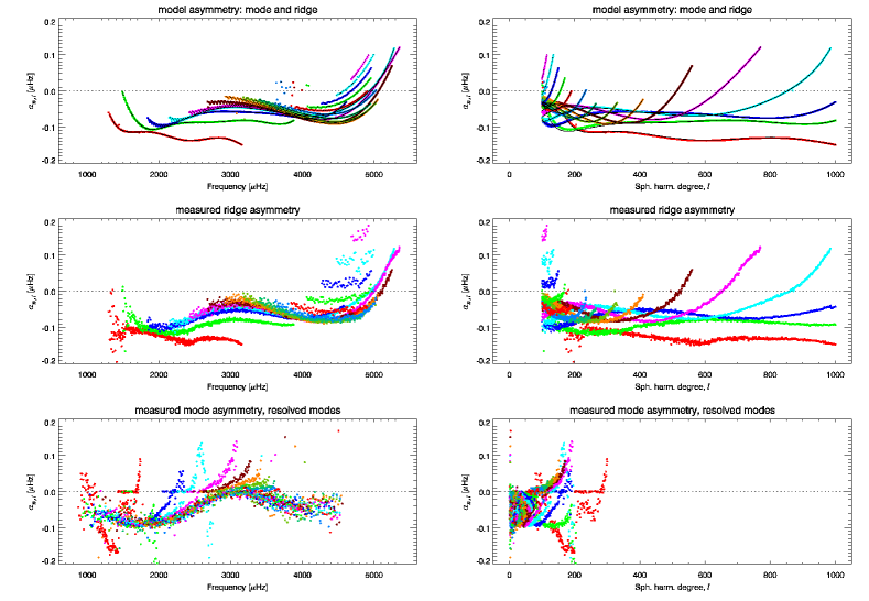
Figure 19: Ridge asymmetry, for zonal modes only, as a function of frequency or degree, left and right panels, respectively. The top panels show the model asymmetry: the input mode asymmetry (black dots) and the resulting ridge asymmetry (colored dots). Our model predicts that, for the zonal modes, the asymmetry of the ridge is essentially the mode asymmetry. The middle panels show the measured ridge asymmetry for intermediate and high degrees. The model asymmetry produced by our iterative process matches (by construction) the observed ridge asymmetry. The bottom panels show the mode asymmetry as measured from fitting resolved modes at low and intermediate degrees. It shows a qualitative similarity – a similar dependence of $\alpha$ on $\nu$ – but a poor quantitative agreement. The color corresponds to the value of the order, $n$.

Figure 20: Comparison between mode asymmetry determined from fitting resolved modes at low and intermediate degrees (crosses and error bars with serifs) and mode asymmetry estimated from ridge fitting at high degrees (dots), for the overlapping region (see Fig. 11). The color corresponds to the value of the order, $n$. Note how, but for some f-modes and most of the $n=1$ modes, the ridge fitting estimates are systematically lower than the individual mode fitting values, although that offset is mostly within $1\,\sigma$.

4.2.3 Amplitude

Figure 21 shows how our model reproduces the observed variation of the ridge amplitude with azimuthal order, although the mode amplitude is constant with $m$. The dominant variation, close to $1+(\frac{m}{\ell})^{2}$, is well reproduced, but the observed values show a departure from the reference model that gets progressively larger at higher degrees. The model also fails to reproduce the asymmetry of the variation of the ridge power amplitude with respect to the azimuthal order, $m$.

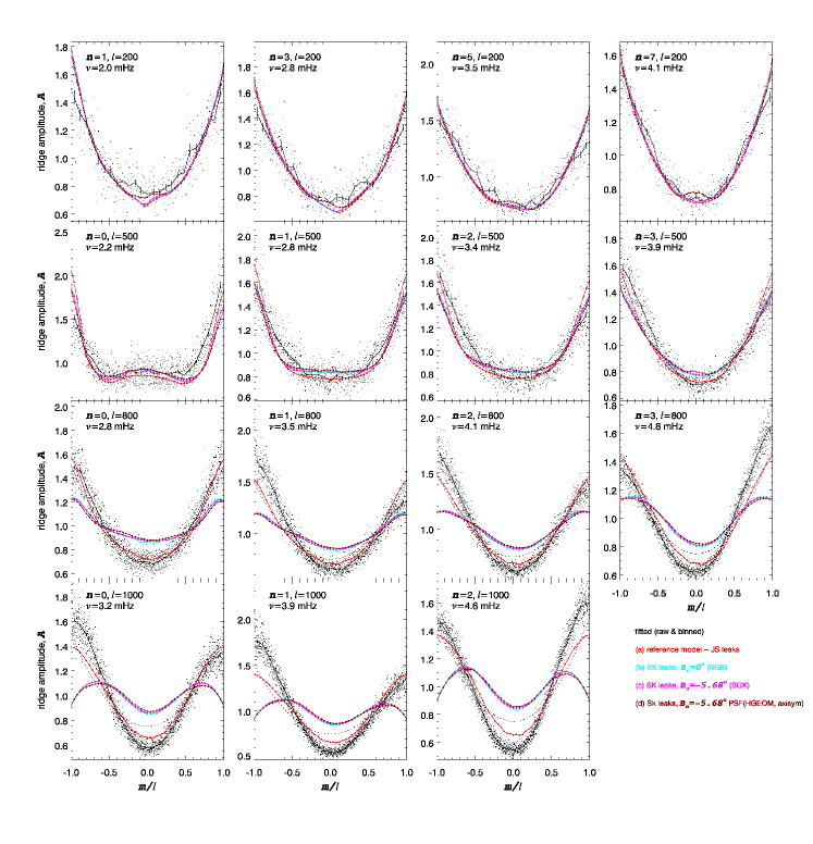
Figure 21: Comparison of ridge amplitude, for a selection of multiplets (as in Figs. 16 and 18), as a function of the ratio $m/\ell$. The dots correspond to individual ridge power amplitude measurements, and the black curves the corresponding binned values. The colored curves correspond to different models of the ridge amplitude, resulting from different models for the leakage matrix. The dotted line corresponds to $1+(\frac{m}{\ell})^{2}$. As for the asymmetry, the models reproduce over all the variation of ridge amplitude with the azimuthal order, while the mode amplitude in the model is constant with $m$. The reference model shows the best match with the observations and the discrepancies between the various model appear at high degrees and high frequencies. Note also how all of the models fail to reproduce the observed asymmetry of the ridge power amplitude.

That figure also illustrates the dependence of the observed variation of the ridge amplitude with $m$ on the leakage matrix used in the modeling. Results from using an independent leakage matrix computation by one of us (SK) are also shown in that figure. Figure 22 shows additional models, where by including various PSFs, we explored the dependence of the ridge amplitude variation with $m$ on the PSF included in the leakage matrix computation.

We computed a set of models using leakage matrices evaluated by including various PSFs. We used the PSF profile determined by HGEOM but instead of using an axisymmetric PSF, we derived an elliptic PSF, $\cal F$, with

$${\cal F}(x,y)=F(r)$$ (49)

where $F(r)$ is the PSF profile determined by HGEOM and where the mapping between $r$, the radius, and the position $(x,y)$ is a rotated ellipse:

$$r=\sqrt{(\frac{x^{\prime}}{a})^{2}+(\frac{y^{\prime}}{b})^{2}}$$ (50)

and

$$x^{\prime} = x\cos\phi-y\sin\phi$$ (51)

$$y^{\prime} = x\sin\phi+y\cos\phi$$ (52)

while $a=1-\eta$ and $b=1+\eta$. Figures 21 and 22 present the variation of the ridge power amplitude with $m$ resulting from the following 8 cases:

• Standard leakage matrix (computed by JS)

• Independent leakage matrix calculation, for $B_{o}=0^{\rm o}$ (computed by SK)

• Independent leakage matrix calculation, for $B_{o}=-5.68^{\rm o}$ (computed by SK)

• As above, plus axisymmetric PSF ($\eta=0,\ \phi=0^{\rm o}$)

• As (c), plus elliptical PSF $\eta=+0.05,\ \phi=0^{\rm o}$

• As (c), plus elliptical PSF $\eta=-0.05,\ \phi=0^{\rm o}$

• As (c), plus elliptical PSF $\eta=-0.10,\ \phi=0^{\rm o}$

• As (c), plus elliptical PSF $\eta=-0.10,\ \phi=20^{\rm o}$

with the first two cases repeated in both figures.

While in none of these models does the amplitude variation with $m$ match the observations, the figures illustrate how the precise variation of $\tilde{A}$ with $m$ at various $\ell$ is quite sensitive to the PSF and suggest that the PSF of MDI is likely to be non-axisymmetrical.

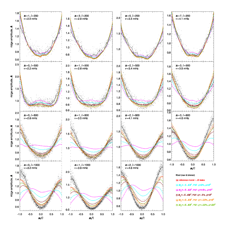
Figure 22: Comparison of scaled ridge amplitude, as a function of the ratio $m/\ell$, scaled as in Fig. 21, for models using different leakage matrices (see text for the description of the models). The dots correspond to individual ridge power amplitude measurements, while the black curves are the corresponding binned values. The colored curves correspond to different models.

A comparison of the zonal amplitudes is shown in Fig. 23, where we show the measured zonal ridge power amplitude and compare it to the ridge amplitude predicted by our model. The ridge zonal amplitudes agree rather well – by construction – since the model input mode amplitudes were adjusted iteratively to achieve such a match. The figure also shows the ratio between the mode amplitude and the ridge amplitude. While below $\ell=300$ the ridge to mode amplitude ratio is a complex function of order and degree, at the higher degrees, that ratio is mostly a function of $\ell$. A reasonable estimate of the mode amplitude can thus be derived using the ratio predicted by our model.

Figure 23: Top panels: comparison of the ridge power amplitude, as a function of frequency (panels on the left) or degree (panels on the right), for zonal modes. The model values (black dots) are compared to the measured ridge amplitude (colored dots). These agree rather well – by construction – since the model input mode amplitudes were adjusted iteratively to achieve such a match. The color corresponds to the value of the order, $n$. Bottom panels: ratio between the mode amplitude and the ridge amplitude estimated from our ridge model.

4.3 Final Correction

The steps used to estimate mode parameters from ridge parameters are summarized as follow. First, for all the singlets we corrected the ridge frequency, by subtracting the ridge to mode offset determined by our model, and propagated the correction uncertainty to the fitting uncertainty. Namely we use Eqs. 35 and 37:

$$\nu_{n,\ell,m} = \tilde{\nu}_{n,\ell,m}-\Delta^{\nu}_{n,\ell,m}$$

$$\sigma^{2}_{\nu_{n,\ell,m}} = \sigma^{2}_{\tilde{\nu}_{n,\ell,m}}+\sigma^{2}_{\Delta^{\nu}_{n,\ell,m}}$$

where $\Delta^{\nu}_{n,\ell,m}$ is defined in Eq. 36 and where $\sigma_{\Delta^{\nu}_{n,\ell,m}}$ is taken to be 1% or 0.1% of $\Delta^{\nu}_{n,\ell,m}$. The zonal frequency for a given multiplet, $\nu_{n,\ell}$, is computed as usual, by fitting Clebsh-Gordan coefficients to the corrected singlets frequencies, $\nu_{n,\ell,m}$.

For the FWHM, asymmetry and amplitude, singlets values for a given multiplet are fitted to a polynomial in $m/\ell$. The zonal value is then estimated as the value at $m=0$ of the fitted polynomial, with the uncertainty associated to the fit. The resulting zonal estimates for the ridge FWHM, asymmetry and amplitude are then corrected to produce zonal mode estimates.

These corrections are:

$$\Gamma^{2}_{n,\ell} = (\Gamma^{E}_{n,\ell})^{2}-W_{N,T}^{2}$$

$$= \tilde{\Gamma}_{n,\ell}^{2}+g\,\tilde{\sigma}_{n,\ell}^{2}-{\cal W}_{n,\ell}^{2}-W_{N,T}^{2}$$

$$\sigma_{\Gamma_{n,\ell}} = \sigma_{\tilde{\Gamma}_{n,\ell}}\tilde{\Gamma}_{n,\ell}/{\cal W}_{n,\ell}$$

$$\alpha_{n,\ell} = \tilde{\alpha}_{n,\ell}-\Delta^{\alpha}_{n,\ell}$$

$$\sigma^{2}_{\alpha_{n,\ell}} = \tilde{\sigma}^{2}_{\alpha_{n,\ell}}+\sigma^{2}_{\Delta^{\alpha}_{n,\ell,m}}$$

$$A_{n,\ell} = \tilde{A}_{n,\ell}/r^{A}_{n,\ell}$$

$$\sigma_{A_{n,\ell}} = \tilde{\sigma}_{r^{A}_{n,\ell}}/r^{A}_{n,\ell}$$

following Eqs. 40, 46, 45 and 48, where $\Delta^{\alpha}_{n,\ell}$ is the small difference between ridge and mode asymmetry predicted by the model of the ridge. The precision on the asymmetry correction, $\sigma_{\Delta^{\alpha}_{n,\ell,m}}$, is negligible and thus is neglected, as the correction itself is minute. The quantity $r^{A}_{n,\ell}$ is the ratio between the ridge and mode amplitude in the model.

These corrections have been carried out using models computed with different leakage matrices and different mode asymmetries. We computed various models since on the one hand, we were unable to produce a good model of the ridge amplitude variation with $m$ that matches the observations, and because on the other hand our estimate of the asymmetry based on ridge fitting does not match the estimates resulting from fitting resolved modes at low and intermediate degrees.

We considered five leakage matrices and two asymmetry models. For the asymmetry, we either allowed it be a bivariate polynomial of frequency and degree, $f_{1}(\nu,\ell)$, and adjusted that function iteratively to match the ridge fitting at intermediate and high degree (as described earlier), or we fixed it to be solely a function of frequency, $f_{2}(\nu)$, set to a polynomial that matches the estimate of the asymmetry resulting from mode fitting at low and intermediate degrees. As for the five leakage matrices, we considered the five cases (a), (b), (c), (d) and (h) described in section 4.2.3.

Table 4: Models Properties: comparison of various models ridge FWHM, amplitude and asymmetry to the corresponding observed values (for $m=0$). The tabulated values are the average and standard deviation of either ratios or differences.

Leakage	Asymmetry
matrix	type	$\tilde{\Gamma}_{M}/\tilde{\Gamma}_{O}$	$\tilde{A}_{M}/\tilde{A}_{O}$	$\tilde{\alpha}_{M}-\tilde{\alpha}_{O}$
(a)	$f_{1}(\nu,\ell)$	0.999 $\pm$ 0.015	1.001 $\pm$ 0.018	0.000 $\pm$ 0.010
(b)	$f_{1}(\nu,\ell)$	0.999 $\pm$ 0.015	0.993 $\pm$ 0.020	0.000 $\pm$ 0.010
(c)	$f_{1}(\nu,\ell)$	1.000 $\pm$ 0.015	0.999 $\pm$ 0.019	0.000 $\pm$ 0.010
(d)	$f_{1}(\nu,\ell)$	1.012 $\pm$ 0.021	1.000 $\pm$ 0.731	0.000 $\pm$ 0.009
(h)	$f_{1}(\nu,\ell)$	1.013 $\pm$ 0.022	1.001 $\pm$ 0.781	0.000 $\pm$ 0.009
(a)	$f_{2}(\nu)$	0.999 $\pm$ 0.015	1.001 $\pm$ 0.018	0.049 $\pm$ 0.052
(b)	$f_{2}(\nu)$	0.999 $\pm$ 0.015	0.992 $\pm$ 0.019	0.049 $\pm$ 0.052
(c)	$f_{2}(\nu)$	1.000 $\pm$ 0.015	0.998 $\pm$ 0.019	0.049 $\pm$ 0.052
(d)	$f_{2}(\nu)$	1.013 $\pm$ 0.021	0.998 $\pm$ 0.728	0.048 $\pm$ 0.052
(h)	$f_{2}(\nu)$	1.014 $\pm$ 0.021	0.999 $\pm$ 0.778	0.048 $\pm$ 0.053

Table 5: Frequency match, singlets: comparison of mode frequencies, at intermediate degree for individual singlets ($\nu_{n,\ell,m}$), determined either by fitting resolved modes or by fitting ridges and correcting for the ridge-to-model offset estimated for various models. The mean and RMS, after a $3\,\sigma$ rejection, are tabulated for raw and scaled differences, as well as the number of overlapping modes and the number of modes kept after the $3\,\sigma$ rejection.

Leakage	Asymmetry	$\Delta\nu_{n,\ell,m}$		$\frac{\Delta\nu_{n,\ell,m}}{\sigma_{\nu_{n,\ell,m}}}$
matrix	type	[$\mu$Hz]	($N,N_{k}$)		($N,N_{k}$)
(a)	$f_{1}(\nu,\ell)$	0.098 $\pm$ 1.656	(73858, 72498)	0.135 $\pm$ 1.409	(73858, 71740)
(b)	$f_{1}(\nu,\ell)$	0.094 $\pm$ 1.656	(73862, 72503)	0.130 $\pm$ 1.408	(73862, 71739)
(c)	$f_{1}(\nu,\ell)$	0.093 $\pm$ 1.654	(73864, 72499)	0.131 $\pm$ 1.406	(73864, 71737)
(d)	$f_{1}(\nu,\ell)$	0.118 $\pm$ 1.660	(73870, 72535)	0.151 $\pm$ 1.410	(73870, 71748)
(h)	$f_{1}(\nu,\ell)$	0.118 $\pm$ 1.659	(73868, 72529)	0.151 $\pm$ 1.410	(73868, 71743)
(a)	$f_{2}(\nu)$	0.086 $\pm$ 1.655	(73860, 72495)	0.123 $\pm$ 1.408	(73860, 71743)
(b)	$f_{2}(\nu)$	0.083 $\pm$ 1.654	(73860, 72490)	0.119 $\pm$ 1.407	(73860, 71739)
(c)	$f_{2}(\nu)$	0.096 $\pm$ 1.739	(65602, 64473)	0.141 $\pm$ 1.387	(65602, 63630)
(d)	$f_{2}(\nu)$	0.108 $\pm$ 1.658	(73869, 72528)	0.143 $\pm$ 1.408	(73869, 71741)
(h)	$f_{2}(\nu)$	0.108 $\pm$ 1.658	(73869, 72526)	0.144 $\pm$ 1.408	(73869, 71739)

Table 6: Frequency match, multiplets: comparison of mode frequencies, as in Table 5, but for multiplets ($\nu_{n,\ell}$).

Leakage	Asymmetry	$\Delta\nu_{n,\ell}$		$\frac{\Delta\nu_{n,\ell}}{\sigma_{\nu_{n,\ell}}}$
matrix	type	[$\mu$Hz]	($N,N_{k}$)		($N,N_{k}$)
(a)	$f_{1}(\nu,\ell)$	0.152 $\pm$ 0.543	(678, 636)	0.806 $\pm$ 2.216	(678, 649)
(b)	$f_{1}(\nu,\ell)$	0.136 $\pm$ 0.543	(678, 636)	0.739 $\pm$ 2.210	(678, 649)
(c)	$f_{1}(\nu,\ell)$	0.137 $\pm$ 0.537	(678, 635)	0.731 $\pm$ 2.201	(678, 649)
(d)	$f_{1}(\nu,\ell)$	0.122 $\pm$ 0.571	(678, 638)	0.682 $\pm$ 2.312	(678, 651)
(h)	$f_{1}(\nu,\ell)$	0.121 $\pm$ 0.573	(678, 638)	0.684 $\pm$ 2.320	(678, 651)
(a)	$f_{2}(\nu)$	0.167 $\pm$ 0.542	(678, 636)	0.871 $\pm$ 2.215	(678, 649)
(b)	$f_{2}(\nu)$	0.153 $\pm$ 0.542	(678, 636)	0.807 $\pm$ 2.205	(678, 649)
(c)	$f_{2}(\nu)$	0.118 $\pm$ 0.541	(596, 560)	0.550 $\pm$ 2.087	(596, 576)
(d)	$f_{2}(\nu)$	0.134 $\pm$ 0.568	(678, 638)	0.725 $\pm$ 2.293	(678, 651)
(h)	$f_{2}(\nu)$	0.135 $\pm$ 0.569	(678, 638)	0.732 $\pm$ 2.296	(678, 651)

Table 4 shows for each of these 10 cases some properties of the resulting models, namely how the widths, amplitudes, and, asymmetries in our modeled ridges match the observations. The widths and asymmetries agree with observations as a result of the iterative process on the model input parameters. By contrast, the modeled asymmetries do not agree with the observations when they are kept as the preset function of frequency, $f_{2}(\nu)$, based on low and intermediate degrees estimates.

Tables 5 and 6 show how well the mode frequencies estimated from ridge fitting, when corrected using these 10 models, match the values measured by fitting resolved modes, for that same overlap range between ridge fitting and resolved mode fitting. The tabulated values are the average and standard deviation of the frequency differences, and the scaled differences ($\Delta\nu/\sigma_{\nu}$), after a $3\,\sigma$ rejection. The number of overlapping modes and the number of these kept after the $3\,\sigma$ rejection are also listed.

Table 5 compares singlets, while Table 6 compares multiplets. These tabulated values are plotted in Fig. 24, where the error bars on the plot are the tabulated RMS. These comparisons show that no model is significantly better amongst these ten when comparing estimate of mode frequencies in the overlapping range between ridge fitting and resolved mode fitting.

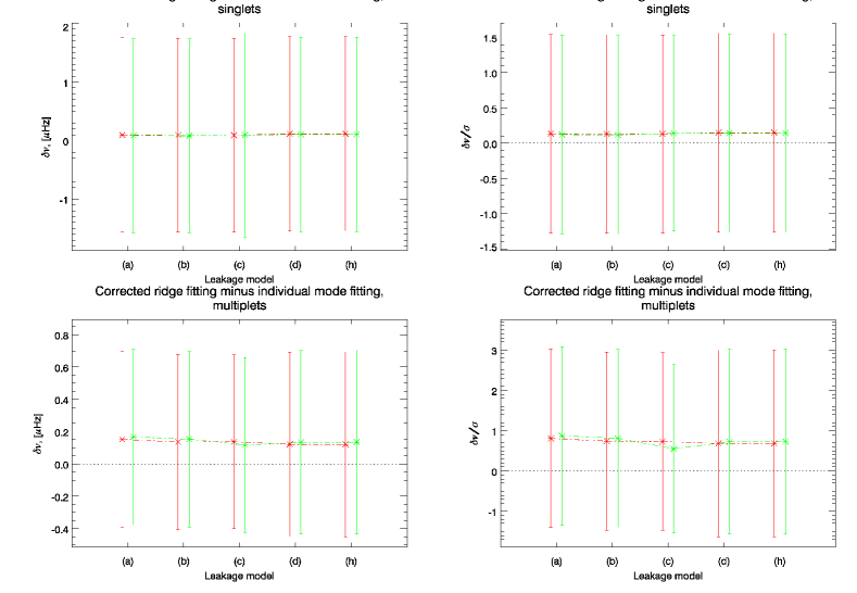
Figure 24: Mean and RMS for frequency differences (left panels) and scaled differences (right panels), between mode frequencies estimated from ridge fitting and values derived from fitting resolved modes, after correcting for the ridge-to-mode offset using different models, as presented in Tables 5 and 6. The top panels correspond to singlets, while the bottom panels correspond to multiplets. The red and green curves are models with the $f_{1}(\nu,\ell)$ or $f_{2}(\nu)$ asymmetry laws, respectively. No model is significanly better, when using this metric.

For illustration, a fraction of the resulting parameters are tabulated in the Appendix in Tables LABEL:tab:multiplets to LABEL:tab:cgCoefs, namely some singlets $(n,\ell,m)$, multiplets $(n,\ell)$, and corresponding Clebsh-Gordan coefficients. The complete tables are available in digital form at
https://www.cfa.harvard.edu/$\sim$sylvain/research/tables/HiL/.

4.4 Remaining Issues

One of the two major remaining issues is our inability to model the MDI instrument PSF. This inability results in incorporating an inadequate leakage matrix, that in turn produces a model of the variation of the ridge amplitude with $m$ that does not match the observations, especially at the higher degrees. It may also explain the mismatch of the variation with $m$ of the ridge width and asymmetry, although at a smaller scale.

Since we have co-eval full disk observations between MDI and HMI, we should be able to derive the MDI PSF from these data. Indeed, on the one hand, the HMI instrument optical characteristics have been carefully measured prior to launch, while on the other hand the higher spatial resolution of HMI will allow us to characterize precisely the PSF of the MDI instrument even without knowing very precisely the PSF of the HMI instrument.

The other remaining issue is the mismatch between the estimates of the mode asymmetry derived from low and intermediate degrees and from intermediate and high degrees. While the introduction of a better PSF for the MDI instrument might slightly change the offset between the mode and ridge asymmetry, the zonal values are unlikely to be much affected. This mismatch is not significant, since the estimates from ridge fitting have large error bars, but it is systematic. We speculate that the difficulty in constraining the background might explain this systematic offset. The background term is likely not symmetric across the ridge, but it is poorly constrained when fitting at intermediate and high degrees since there is almost no free spectral range between the ridges. It is thus conceivable that the measured ridge asymmetry might be contaminated by the local slope of the unconstrained background across the ridge.

Other remaining issues are whether our model of the image distortion and its orientation (the effective $P$ angle) are taken into account at the required precision at the spatial decomposition step. These may be responsible at some level for the mismatch between our models and the observations of the variation of the ridge amplitude with $m$.

5 Conclusions

We have successfully derived and implemented a procedure to estimate mode parameters for high degree modes, using ridge fitting. We are able to derive not only frequencies, but widths, asymmetries and amplitudes. For a range of degrees we have overlapping mode determination derived from ridge fitting and from resolved mode fitting. Thus we could quantitatively assess the precision of our method and found no residual significant differences.

Our extensive analysis of the precision of our correction scheme shows that the correction precision is substantially better than the fitting precision, but for two caveats: one is the residual, although not significant, discrepancy between the determination of the asymmetry from ridge fitting and from mode fitting that prevents us from asserting that our model of the mode asymmetry is well constrained. The other is the contribution of the instrumental PSF, through the leakage matrix, that for MDI we are unable to constrain from the data and for which we do not have a valid pre flight determination.

In both cases, our inability to constrain these properties results in some potential remaining systematic errors in the corrected parameters. We are unable to find an objective metric to select a best model. The PSF “problem” can, and we hope will, be solved by analyzing co-eval data acquired by HMI and MDI.

As for implications on other data sets, the optimistic view is to expect that when analyzing HMI data, an instrument that delivers full resolution full disk observations at all times, the instrument PSF will be shown to be well known. Applying our methodology to these data would allow us to confirm this. For the GONG data, we have to be realistic and recognize that the effective PSF is likely to also be a problem, since the contribution of the atmosphere needs to be taken into consideration, and one has to merge data from six different instruments.

Appendix: Tables

This appendix presents a subset of the mode characteristics resulting from ridge fitting after correcting them according to the procedure described in this paper. We show in Table LABEL:tab:singlets a selection of singlets $(n,\ell,m)$ (i.e., for 11 equispaced values of $m$, 3 three values of $n$ and for values of $\ell$ that are mutiples of 100). The blank entries correspond to cases where the fitting failed. A selection of multiplets $(n,\ell)$ is presented in Table LABEL:tab:multiplets, for all $n$ and for values of $\ell$ that are mutiple of 100; and the corresponding Clebsh-Gordan first three even coefficients in Table LABEL:tab:cgCoefs. The complete tables are available in digital form at
https://www.cfa.harvard.edu/$\sim$sylvain/research/tables/HiL/.

Table 7: Selected subset of singlets.

$m$	$\nu_{n,\ell,m}$	$\sigma_{\nu_{n,\ell,m}}$	$\Delta^{\nu}_{n,\ell,m}$	$\nu_{n,\ell,m}$	$\sigma_{\nu_{n,\ell,m}}$	$\Delta^{\nu}_{n,\ell,m}$	$\nu_{n,\ell,m}$	$\sigma_{\nu_{n,\ell,m}}$	$\Delta^{\nu}_{n,\ell,m}$
$\ell=100$	$n=1$			$n=8$			$n=14$
-100				3360.08	2.66	0.90	4665.92		0.37
-80	1463.21	0.98	3.66	3366.17	2.22	0.67	4655.25	2.70	0.16
-60	1464.67	0.66	3.27	3372.48	3.48	0.42	4651.68	4.59	-0.36
-40				3382.38	2.11	-0.82	4677.26	3.54	-0.64
-20	1486.21	1.85	3.44	3391.81	2.91	0.14	4671.52	4.06	-0.33
0				3396.76	3.36	1.04	4677.05	3.73	0.41
20	1493.28	0.05	5.03	3405.98	2.65	1.60	4689.71	3.92	1.18
40				3415.19	3.54	2.01	4696.68	3.25	1.50
60	1509.91	1.81	5.31	3421.46	3.17	1.65	4706.72	3.38	1.05
80				3429.23	2.31	1.09	4716.58	3.48	0.57
100				3438.31	3.10	0.91	4712.56	5.67	0.38
$\ell=200$	$n=0$			$n=5$			$n=9$
-200	1340.61	0.23	3.17	3387.44	0.37	1.32	4628.16	2.30	1.21
-160	1358.98	0.66	2.80	3409.92	0.69	0.90	4651.74	2.73	0.82
-120	1377.24	1.36	1.80	3426.47	1.66	-0.12	4671.43	1.82	-0.11
-80				3441.62	0.86	-0.82	4685.10	1.97	-0.81
-40	1412.51	0.94	2.04	3459.80	0.91	-0.14	4701.94	2.23	-0.27
0	1422.94	0.53	3.64	3475.29	0.54	1.39	4719.60	4.79	1.20
40	1440.79	1.42	5.23	3487.78	0.57	2.91	4731.66	1.99	2.68
80	1460.71	0.69	6.09	3502.31	1.73	3.66	4749.17	2.02	3.21
120	1474.25	1.32	5.72	3523.42	1.32	3.00	4767.42	2.14	2.47
160	1495.95	0.54	4.61	3540.49	1.12	1.92	4787.40	3.89	1.61
200	1511.24	0.31	4.06	3556.95	0.88	1.49	4799.06	1.86	1.28
$\ell=300$	$n=0$			$n=4$			$n=7$
-300	1615.85	0.47	2.50	3524.09	0.26	1.31	4706.00	3.44	1.55
-240	1644.04	0.43	1.91	3551.80	0.38	0.72	4735.39	4.34	1.03
-180	1671.84	0.44	0.08	3580.30	0.76	-0.83	4763.52	3.70	-0.27
-120	1696.78	0.37	-0.58	3604.94	0.55	-1.87	4784.36	2.70	-1.29
-60	1720.06	0.35	0.61	3629.08	0.51	-0.91	4807.83	2.82	-0.56
0	1742.65	0.47	2.95	3653.42	1.44	1.38	4831.62	3.32	1.55
60	1763.32	0.52	5.28	3676.21	1.00	3.67	4855.95	3.97	3.66
120	1787.29	0.41	6.56	3696.90	0.83	4.67	4886.94	6.23	4.34
180	1813.92	0.32	6.03	3720.38	0.55	3.64	4904.75	3.31	3.29
240	1839.47	0.40	4.18	3752.99	0.39	2.13	4930.28	3.72	2.13
300	1867.36	0.50	3.36	3776.91	0.44	1.54	4957.49	4.56	1.68
$\ell=400$	$n=0$			$n=3$			$n=6$
-400	1839.45	0.34	2.11	3439.71	1.13	1.31	4816.28	8.92	1.96
-320	1878.15	0.25	1.27	3481.20	0.78	0.55	4872.71	5.22	1.27
-240	1914.15	0.61	-1.56	3516.83	0.59	-1.56	4891.44	9.35	-0.43
-160	1948.60	0.23	-2.11	3550.95	0.42	-2.80	4937.41	5.64	-1.75
-80	1978.15	0.33	-0.49	3581.83	0.48	-1.56	4966.79	4.67	-0.80
0	2007.35	0.28	2.55	3617.48	0.66	1.43	5010.96	7.36	1.97
80	2037.30	0.34	5.59	3644.29	0.50	4.39	5031.16	5.16	4.71
160	2069.90	0.26	7.28	3674.82	0.49	5.62	5058.36	4.26	5.53
240	2103.62	0.35	6.78	3706.99	0.53	4.34	5095.35	6.32	4.14
320	2138.66	0.41	4.10	3741.46	1.07	2.40	5122.64	6.07	2.70
400	2176.16	0.27	2.97	3779.39	0.56	1.63	5158.84	5.39	2.12
$\ell=500$	$n=0$			$n=3$			$n=5$
-500	2032.10	0.32	1.86	3721.59	1.21	1.40	4779.20	6.69	2.12
-400	2079.39	0.41	0.78	3776.78	1.62	0.51	4850.66	8.85	1.29
-300	2126.49	0.85	-2.80	3819.99	1.16	-1.89	4892.13	5.98	-0.83
-200	2168.71	0.37	-3.39	3864.13	1.22	-3.45	4944.70	7.41	-2.49
-100	2206.01	0.27	-1.35	3900.53	1.19	-2.04	4971.54	6.02	-1.30
0	2241.99	0.22	2.29	3936.12	1.30	1.53	5010.78	7.64	2.17
100	2280.01	0.27	5.96	3974.21	1.22	5.06	5044.81	5.69	5.63
200	2317.49	0.49	8.05	4011.97	0.86	6.30	5088.53	6.62	6.65
300	2358.19	0.72	7.48	4052.67	1.14	4.62	5121.74	7.40	4.92
400	2404.15	1.22	4.11	4096.97	1.84	2.57	5168.51	5.48	3.10
500	2451.90	0.26	2.71	4145.79	0.96	1.74	5212.01	7.12	2.33
$\ell=600$	$n=0$			$n=2$			$n=4$
-600	2200.85	0.33	1.69	3375.48	0.59	1.45	4569.96	5.64	1.98
-480	2257.50	0.48	0.50	3434.14	0.48	0.30	4639.09	5.27	0.96
-360	2314.26	1.17	-3.44	3489.62	1.31	-2.90	4695.63	6.61	-1.64
-240	2363.97	1.75	-4.38	3541.13	0.76	-4.57	4746.18	5.60	-3.63
-120	2410.97	0.56	-2.05	3588.47	0.94	-2.68	4780.55	4.67	-2.16
0	2454.05	0.35	2.12	3627.75	0.79	1.64	4825.35	4.58	2.07
120	2498.71	0.56	6.32	3670.88	1.29	5.92	4878.69	6.53	6.28
240	2541.67	1.75	8.65	3723.76	1.30	7.58	4933.80	6.08	7.50
360				3772.76	1.00	5.73	4963.75	4.89	5.41
480	2649.34	1.08	4.04	3825.62	1.10	3.01	5028.84	4.75	3.22
600	2704.88	0.42	2.54	3881.58	0.65	1.91	5084.24	4.74	2.25
$\ell=700$	$n=0$			$n=2$			$n=4$
-700	2355.80	0.67	1.59	3585.34	1.18	1.52	4859.54	17.31	2.51
-560	2422.35	0.76	0.32	3655.52	1.27	0.18	4907.81	10.03	1.27
-420	2484.73	1.92	-3.75	3721.56	2.49	-3.38	4978.88	10.58	-1.82
-280	2545.93	0.68	-5.24	3780.02	2.10	-5.43	5035.02	11.13	-4.16
-140	2598.77	0.35	-2.71	3834.58	1.20	-3.33	5099.94	9.38	-2.44
0	2650.02	0.36	2.00	3886.56	1.52	1.76	5143.83	11.42	2.66
140	2700.27	0.88	6.73	3932.49	1.61	6.75	5193.52	8.96	7.67
280	2754.29	0.97	9.10	3990.67	1.69	8.46	5257.80	9.74	9.03
420	2810.04	2.09	7.60	4042.58	1.67	6.16	5299.17	11.27	6.55
560	2877.00	0.97	3.93	4114.32	1.71	3.24	5383.13	10.16	3.98
700	2941.49	0.40	2.42	4175.79	1.34	1.99	5433.74	7.97	2.79
$\ell=800$	$n=0$			$n=2$			$n=3$
-800	2490.31	1.00	1.55	3786.28	2.67	1.64	4455.38	5.41	2.07
-640	2570.26	1.06	0.12	3871.52	1.92	0.03	4534.01	4.57	0.51
-480	2642.63	1.79	-4.16	3947.30	2.58	-3.95	4610.64	5.26	-3.19
-320	2708.33	1.17	-6.07	4011.97	1.79	-6.36	4667.91	5.59	-5.80
-160	2769.17	0.87	-3.48	4072.83	2.29	-4.05	4739.06	6.38	-3.71
0	2830.75	0.86	1.98	4132.14	1.81	1.82	4792.00	5.11	2.17
160	2890.48	0.84	7.37	4185.19	2.18	7.71	4849.83	5.39	8.13
320	2948.68	1.21	9.67	4256.81	2.41	9.51	4918.18	5.76	9.73
480	3020.75	1.53	7.62	4320.01	2.91	6.77	4986.92	5.49	6.87
640	3088.17	1.00	3.97				5065.60	6.78	3.85
800	3165.50	1.01	2.37	4464.78	1.62	2.11	5134.08	5.31	2.42
$\ell=900$	$n=0$			$n=2$			$n=3$
-900	2620.96	1.43	1.55	3997.98	3.27	1.81	4688.00	11.95	2.49
-720	2705.26	1.35	-0.15	4077.75	3.79	-0.12	4765.47	8.70	0.60
-540	2790.34	2.28	-4.84	4159.38	4.18	-4.60	4845.57	8.97	-3.67
-360	2862.60	1.30	-7.20	4234.49	3.13	-7.41	4913.34	11.78	-6.63
-180	2935.24	1.60	-4.34	4309.82	3.42	-4.83	5004.43	10.60	-4.24
0	3003.06	1.37	1.98	4374.78	3.11	2.01	5062.39	9.84	2.62
180	3061.50	1.52	8.21	4442.40	3.57	8.85	5125.96	10.22	9.54
360	3128.93	1.86	10.55	4506.11	3.86	10.77	5187.44	8.42	11.31
540	3203.81	2.29	7.95	4582.98	3.89	7.60	5274.33	9.25	8.04
720	3291.54	1.53	4.15	4661.43	3.29	3.99	5351.52	9.20	4.55
900	3372.62	1.52	2.38	4749.11	3.30	2.27	5439.97	8.28	2.84
$\ell=1000$	$n=0$			$n=1$			$n=2$
-1000				3454.34	2.11	1.75	4183.54	4.48	2.04
-800	2837.09	2.54	-0.33	3555.08	4.40	-0.61	4280.47	4.26	-0.22
-600	2921.95	3.30	-5.48	3649.84	3.14	-6.06	4386.49	4.47	-5.31
-400	3006.85	2.90	-8.26	3730.87	2.60	-8.87	4454.42	4.30	-8.52
-200	3083.96	2.10	-5.36	3804.57	2.11	-5.77	4538.02	4.35	-5.69
0	3156.62	3.21	2.07	3879.78	2.21	2.03	4613.72	4.22	2.24
200	3225.57	2.16	9.34	3951.35	3.21	9.66	4683.41	5.59	9.99
400	3308.10	2.25	11.68	4030.11	2.58	12.08	4758.74	5.90	12.31
600	3387.98	3.00	8.61	4111.34	2.87	8.67	4841.74	4.19	8.74
800	3483.79	2.44	4.59	4198.87	2.31	4.45
1000	3574.75	2.12	2.50	4296.71	1.80	2.36	5029.08	4.80	2.49

Table 8: Selected subset of multiplets.

$n$	$\ell$	$\nu_{n,\ell}$	$\sigma_{\nu_{n,\ell}}$	$\Delta^{\nu}_{n,\ell}$	$\tilde{\Gamma}_{n,\ell}$	$\tilde{\alpha}_{n,\ell}$	$\tilde{A}_{n,\ell}$	$\Gamma_{n,\ell}$	$\sigma_{\Gamma_{n,\ell}}$	$\alpha_{n,\ell}$	$\sigma_{\alpha_{n,\ell}}$	$A_{n,\ell}$	$\sigma_{A_{n,\ell}}$
1	100	1490.27	2.03	4.21	15.52	-0.086	5.67e-04	$\leq 1.96$	2.23	-0.095	0.068	7.66e-03	7.26e-04
2	100	1845.44	0.33	3.37	14.74	-0.132	4.78e-03	$\leq 1.96$	0.80	-0.134	0.023	4.89e-02	1.59e-03
3	100	2146.16	0.39	3.40	17.93	-0.100	1.85e-02	$\leq 1.96$	0.97	-0.107	0.022	1.47e-01	4.14e-03
4	100	2423.24	0.37	2.25	19.84	-0.026	5.48e-02	$\leq 1.96$	0.98	-0.039	0.018	4.11e-01	9.46e-03
5	100	2678.75	0.32	2.16	21.52	0.004	1.26e-01	$\leq 1.96$	1.35	-0.019	0.015	1.11e+00	2.75e-02
6	100	2928.89	0.43	1.80	23.76	-0.005	2.28e-01	$\leq 1.96$	1.58	-0.031	0.020	2.13e+00	4.38e-02
7	100	3167.81	0.41	1.27	25.77	-0.031	2.50e-01	$\leq 1.96$	1.70	-0.048	0.017	2.27e+00	4.53e-02
8	100	3398.58	0.29	1.04	28.70	-0.041	1.40e-01	$\leq 1.96$	1.69	-0.050	0.011	1.18e+00	2.44e-02
9	100	3623.47	0.29	0.80	31.36	-0.021	6.20e-02	$\leq 1.96$	1.93	-0.025	0.010	4.58e-01	8.19e-03
10	100	3845.15	0.32	0.67	36.51	-0.038	2.69e-02	12.68	1.86	-0.037	0.010	1.63e-01	2.80e-03
11	100	4061.31	0.38	0.53	41.39	-0.025	1.35e-02	17.45	2.32	-0.025	0.011	6.66e-02	1.00e-03
12	100	4272.21	0.47	0.48	50.24	0.013	7.06e-03	29.43	2.55	0.012	0.014	2.96e-02	4.81e-04
13	100	4479.18	0.55	0.49	58.60	0.096	3.85e-03	38.57	3.51	0.092	0.019	1.39e-02	2.41e-04
14	100	4667.48	1.04	0.41	68.51	0.134	2.31e-03	48.72	5.21	0.130	0.034	7.35e-03	2.10e-04
0	200	1429.52	0.61	3.64	9.67	-0.077	5.12e-04	$\leq 1.96$	0.42	-0.085	0.044	3.82e-03	1.61e-04
1	200	1967.68	0.09	2.43	10.01	-0.119	1.32e-02	$\leq 1.96$	0.15	-0.127	0.008	7.28e-02	1.41e-03
2	200	2392.48	0.11	2.20	12.94	-0.080	7.03e-02	4.94	0.21	-0.085	0.007	3.77e-01	6.41e-03
3	200	2765.51	0.13	1.91	13.77	-0.040	2.40e-01	4.05	0.25	-0.042	0.008	1.36e+00	2.11e-02
4	200	3131.93	0.13	1.67	15.47	-0.039	3.85e-01	4.54	0.32	-0.040	0.008	2.18e+00	3.46e-02
5	200	3474.16	0.14	1.39	19.42	-0.054	1.74e-01	8.43	0.40	-0.057	0.007	8.01e-01	1.24e-02
6	200	3804.14	0.18	1.18	26.00	-0.077	5.01e-02	15.23	0.54	-0.081	0.006	1.73e-01	2.56e-03
7	200	4119.44	0.21	1.12	39.31	-0.080	1.39e-02	30.45	0.63	-0.083	0.005	3.86e-02	4.47e-04
8	200	4423.91	0.23	1.16	52.94	-0.077	5.12e-03	44.71	1.11	-0.079	0.005	1.30e-02	1.29e-04
9	200	4717.78	0.34	1.20	73.88	-0.072	2.11e-03	66.73	2.01	-0.073	0.008	5.13e-03	5.38e-05
0	300	1742.04	0.06	2.95	8.42	-0.099	3.27e-03	$\leq 1.96$	0.10	-0.102	0.008	1.38e-02	2.46e-04
1	300	2286.96	0.07	2.02	11.14	-0.096	3.84e-02	5.80	0.13	-0.102	0.005	1.16e-01	1.74e-03
2	300	2779.88	0.08	1.71	13.43	-0.067	1.77e-01	7.91	0.19	-0.072	0.005	5.44e-01	7.96e-03
3	300	3234.66	0.10	1.58	14.97	-0.046	2.70e-01	7.73	0.24	-0.050	0.005	9.16e-01	1.23e-02
4	300	3652.31	0.11	1.38	21.80	-0.075	8.39e-02	15.28	0.32	-0.078	0.005	2.35e-01	2.92e-03
5	300	4062.44	0.15	1.36	39.85	-0.083	1.59e-02	35.14	0.42	-0.085	0.004	3.85e-02	3.76e-04
6	300	4456.84	0.21	1.46	64.60	-0.088	4.08e-03	60.84	0.81	-0.089	0.004	9.50e-03	7.66e-05
7	300	4834.19	0.33	1.55	101.35	-0.077	1.32e-03	98.18	1.75	-0.078	0.006	3.03e-03	2.20e-05
0	400	2008.28	0.05	2.55	9.18	-0.119	8.54e-03	3.54	0.09	-0.120	0.005	2.31e-02	3.25e-04
1	400	2556.36	0.08	1.91	14.12	-0.105	5.37e-02	10.15	0.16	-0.108	0.004	1.27e-01	1.42e-03
2	400	3088.70	0.08	1.59	16.25	-0.054	1.60e-01	12.11	0.19	-0.057	0.004	4.02e-01	4.55e-03
3	400	3613.61	0.11	1.43	25.32	-0.066	6.71e-02	21.80	0.26	-0.068	0.004	1.64e-01	1.80e-03
4	400	4105.68	0.14	1.52	47.15	-0.086	1.07e-02	44.14	0.40	-0.087	0.003	2.49e-02	2.06e-04
5	400	4561.20	0.23	1.67	84.02	-0.069	2.29e-03	81.82	0.78	-0.070	0.004	5.27e-03	3.53e-05
6	400	5000.85	0.41	1.97	147.63	-0.026	6.65e-04	145.72	1.86	-0.027	0.007	1.52e-03	8.75e-06
0	500	2242.80	0.07	2.29	11.41	-0.134	1.23e-02	7.03	0.13	-0.133	0.004	2.63e-02	2.75e-04
1	500	2801.33	0.09	1.87	19.34	-0.083	4.81e-02	16.38	0.19	-0.085	0.004	1.06e-01	1.01e-03
2	500	3367.17	0.09	1.59	23.55	-0.058	6.97e-02	20.68	0.21	-0.059	0.003	1.64e-01	1.55e-03
3	500	3936.25	0.14	1.53	44.75	-0.071	1.39e-02	42.71	0.32	-0.072	0.003	3.25e-02	2.55e-04
4	500	4493.43	0.19	1.72	88.71	-0.075	2.13e-03	87.27	0.60	-0.076	0.003	4.97e-03	2.78e-05
5	500	5009.82	0.40	2.17	162.85	-0.035	4.86e-04	161.52	1.57	-0.035	0.006	1.14e-03	5.18e-06
0	600	2454.82	0.08	2.12	16.35	-0.140	1.15e-02	13.26	0.18	-0.139	0.004	2.29e-02	2.13e-04
1	600	3031.40	0.09	1.85	25.17	-0.077	3.36e-02	22.94	0.21	-0.078	0.003	7.52e-02	6.17e-04
2	600	3630.70	0.11	1.64	34.98	-0.069	2.28e-02	32.93	0.25	-0.070	0.003	5.43e-02	4.18e-04
3	600	4235.20	0.16	1.69	72.06	-0.077	3.45e-03	70.76	0.39	-0.077	0.002	8.35e-03	4.99e-05
4	600	4832.45	0.31	2.07	149.45	-0.033	5.67e-04	148.53	0.90	-0.033	0.005	1.39e-03	5.88e-06
0	700	2649.22	0.09	2.00	24.14	-0.136	8.61e-03	22.02	0.20	-0.136	0.003	1.79e-02	1.43e-04
1	700	3251.42	0.10	1.87	34.92	-0.080	1.69e-02	33.19	0.23	-0.080	0.003	4.04e-02	2.76e-04
2	700	3884.80	0.12	1.76	51.83	-0.076	6.54e-03	50.47	0.30	-0.076	0.002	1.66e-02	1.08e-04
3	700	4520.80	0.19	1.95	107.58	-0.062	9.60e-04	106.75	0.51	-0.062	0.002	2.50e-03	1.20e-05
4	700	5145.12	0.48	2.66	229.68	0.041	1.76e-04	229.02	1.67	0.041	0.005	4.64e-04	1.72e-06
0	800	2829.18	0.10	1.98	36.11	-0.128	5.28e-03	34.69	0.24	-0.128	0.003	1.22e-02	8.65e-05
1	800	3464.52	0.11	1.87	46.83	-0.080	7.05e-03	45.49	0.26	-0.080	0.002	1.87e-02	1.19e-04
2	800	4131.67	0.15	1.82	74.24	-0.068	1.92e-03	73.14	0.33	-0.068	0.002	5.38e-03	2.91e-05
3	800	4795.55	0.26	2.17	152.07	-0.019	2.97e-04	151.31	0.69	-0.019	0.003	8.51e-04	3.28e-06
0	900	2997.09	0.12	1.98	52.14	-0.129	2.84e-03	51.07	0.28	-0.129	0.002	7.60e-03	4.52e-05
1	900	3672.76	0.13	1.95	61.91	-0.087	2.62e-03	60.89	0.30	-0.087	0.002	7.95e-03	4.78e-05
2	900	4373.29	0.17	2.01	102.63	-0.060	5.84e-04	101.71	0.41	-0.061	0.002	1.86e-03	9.06e-06
3	900	5062.73	0.39	2.62	221.50	0.022	9.63e-05	220.86	1.15	0.022	0.004	3.14e-04	1.10e-06
0	1000	3154.77	0.13	2.07	75.30	-0.138	1.35e-03	74.84	0.36	-0.138	0.002	4.31e-03	2.47e-05
1	1000	3877.95	0.13	2.03	81.52	-0.091	9.07e-04	80.89	0.34	-0.091	0.002	3.26e-03	1.85e-05
2	1000	4610.80	0.20	2.24	135.00	-0.040	1.83e-04	134.58	0.53	-0.040	0.002	6.88e-04	3.04e-06

Table 9: Selected subset of Clebsch-Gordan coefficients.

$n$	$\ell$	$\nu_{n,\ell}$	$cg_{n,\ell}(1)$	$cg_{n,\ell}(3)$	$cg_{n,\ell}(5)$	$\sigma_{cg_{n,\ell}(1)}$	$\sigma_{cg_{n,\ell}(3)}$	$\sigma_{cg_{n,\ell}(5)}$
1	100	1490.3	359.10	9.53	-5.98	11.17	9.33	7.30
2	100	1845.4	361.01	-4.29	1.75	2.33	1.61	1.19
3	100	2146.2	357.59	-7.02	-0.07	2.48	1.74	1.32
4	100	2423.2	361.39	-4.51	-1.67	2.46	1.65	1.29
5	100	2678.7	357.92	-10.23	-3.23	2.06	1.40	1.09
6	100	2928.9	360.87	-5.56	-0.47	2.75	1.83	1.51
7	100	3167.8	357.69	-11.04	-0.33	2.70	1.71	1.41
8	100	3398.6	357.18	-9.05	-1.71	1.85	1.25	0.98
9	100	3623.5	360.31	-10.61	-2.20	1.85	1.25	1.02
10	100	3845.1	355.93	-9.65	0.01	2.00	1.36	1.10
11	100	4061.3	359.91	-7.78	-0.17	2.46	1.66	1.31
12	100	4272.2	359.63	-9.27	-1.66	2.97	2.07	1.63
13	100	4479.2	358.03	-6.85	-3.21	3.62	2.41	1.86
14	100	4667.5	370.72	-15.02	-12.33	10.51	5.29	1.53
0	200	1429.5	348.78	-1.59	-0.11	1.94	1.31	1.17
1	200	1967.7	356.67	-8.22	-0.86	0.29	0.18	0.15
2	200	2392.5	359.23	-7.53	-0.86	0.35	0.22	0.18
3	200	2765.5	358.37	-7.23	-0.37	0.40	0.27	0.22
4	200	3131.9	360.23	-7.62	-0.66	0.42	0.28	0.23
5	200	3474.2	360.72	-7.16	-0.38	0.45	0.30	0.24
6	200	3804.1	359.57	-7.94	-0.19	0.56	0.39	0.30
7	200	4119.4	361.26	-8.11	-0.70	0.66	0.43	0.34
8	200	4423.9	360.44	-7.15	-0.08	0.75	0.49	0.38
9	200	4717.8	362.64	-6.11	-1.17	1.08	0.73	0.57
0	300	1742.0	356.22	-7.48	-0.70	0.14	0.09	0.07
1	300	2287.0	356.46	-7.73	-0.52	0.16	0.10	0.08
2	300	2779.9	356.75	-7.88	-0.73	0.19	0.12	0.10
3	300	3234.7	357.20	-8.02	-0.63	0.21	0.14	0.11
4	300	3652.3	357.63	-7.68	-0.78	0.25	0.16	0.13
5	300	4062.4	358.19	-7.93	-0.83	0.32	0.21	0.17
6	300	4456.8	359.71	-7.34	-0.38	0.46	0.31	0.25
7	300	4834.2	361.43	-5.55	-0.58	0.71	0.48	0.37
0	400	2008.3	356.08	-7.42	-0.60	0.09	0.06	0.04
1	400	2556.4	355.37	-7.78	-0.49	0.13	0.08	0.07
2	400	3088.7	355.87	-8.15	-0.52	0.14	0.09	0.07
3	400	3613.6	356.42	-8.20	-0.39	0.18	0.11	0.09
4	400	4105.7	357.62	-8.18	-0.77	0.23	0.16	0.12
5	400	4561.2	359.08	-7.17	-0.48	0.37	0.25	0.20
6	400	5000.9	360.31	-5.78	-0.30	0.65	0.44	0.35
0	500	2242.8	355.21	-7.50	-0.43	0.10	0.05	0.04
1	500	2801.3	355.03	-8.00	-0.47	0.12	0.07	0.06
2	500	3367.2	355.24	-8.33	-0.53	0.13	0.08	0.06
3	500	3936.3	355.95	-7.98	-0.42	0.19	0.12	0.10
4	500	4493.4	356.84	-8.23	-0.72	0.25	0.17	0.13
5	500	5009.8	357.52	-7.45	-0.61	0.51	0.34	0.28
0	600	2454.8	354.61	-7.77	-0.46	0.10	0.06	0.04
1	600	3031.4	354.45	-8.11	-0.42	0.11	0.07	0.05
2	600	3630.7	355.22	-8.01	-0.51	0.12	0.08	0.06
3	600	4235.2	356.39	-7.88	-0.59	0.17	0.11	0.09
4	600	4832.5	357.64	-7.47	-0.75	0.34	0.22	0.18
0	700	2649.2	354.23	-7.89	-0.45	0.10	0.06	0.04
1	700	3251.4	354.49	-8.10	-0.55	0.10	0.06	0.05
2	700	3884.8	355.17	-8.16	-0.49	0.11	0.07	0.06
3	700	4520.8	356.03	-7.93	-0.74	0.17	0.11	0.09
4	700	5145.1	356.71	-7.23	-0.50	0.44	0.29	0.24
0	800	2829.2	353.78	-8.12	-0.44	0.09	0.06	0.04
1	800	3464.5	354.34	-8.15	-0.48	0.09	0.06	0.05
2	800	4131.7	355.22	-8.07	-0.50	0.12	0.08	0.06
3	800	4795.6	356.77	-7.71	-0.55	0.21	0.14	0.11
0	900	2997.1	353.58	-8.20	-0.43	0.09	0.06	0.04
1	900	3672.8	354.33	-8.27	-0.56	0.09	0.06	0.05
2	900	4373.3	355.42	-8.29	-0.69	0.12	0.08	0.06
3	900	5062.7	357.41	-7.60	-0.72	0.28	0.19	0.15
0	1000	3154.8	353.46	-8.29	-0.57	0.08	0.06	0.04
1	1000	3878.0	354.16	-8.38	-0.55	0.09	0.06	0.05
2	1000	4610.8	354.82	-8.44	-0.71	0.13	0.09	0.07

References

- Eff-Darwich & Korzennik (2012) Eff-Darwich, A., & Korzennik, S. G. 2012, “The Dynamics of the Solar Radiative Zone”, Sol. Phys., DOI: 10.1007/s11207-012-0048-z
- Fahlman & Ulrych (1982) Fahlman, G. G., & Ulrych, T. J. 1982, “New Method for Estimating the Power Spectrum of Gapped Data”, MNRAS, 199, 53-66
- Hill et al. (1996) Hill, F., et al. 1996, “The Solar Acoustic Spectrum and Eigenmode Parameters”, Science, 272, 1292
- Korzennik (1990) Korzennik, S. G. 1990, “Seismic analysis of the sun from intermediate and high-degree p-modes”, Ph.D. Thesis,
- Korzennik et al. (1990) Korzennik, S. G., Cacciani, A., Rhodes, E. J., & Ulrich, R. K. 1990, “Contribution of High-Degree Frequency Splittings to the Inversions of the Solar Rotation Rate”, Progress of Seismology of the Sun and Stars, 367, 341
- Korzennik et al. (1993) Korzennik, S. G., Cacciani, A., & Rhodes, E. J., Jr. 1993, “Towards a Better Determination of Frequency Splittings at Intermediate and High Degree Modes - Preliminary Results of Sectoral Frequency Splittings from a 90-DAY Observing Run”, GONG 1992. Seismic Investigation of the Sun and Stars, 42, 201
- Korzennik (1998) Korzennik, S. 1998, “Structure and Dynamics of the Interior of the Sun and Sun-like Stars”, Structure and Dynamics of the Interior of the Sun and Sun-like Stars, 418,
- Korzennik & Eff-Darwich (1999) Korzennik, S. G., & Eff-Darwich, A. 1999, “Solar Rotation Near the Surface: The Outer 1%”, SOHO-9 Workshop on Helioseismic Diagnostics of Solar Convection and Activity, 9,
- Korzennik et al. (2003) Korzennik, S. G., Rabello-Soares, C., & Schou, J. 2003, “On the characterization of high-degree modes: a lesson from MDI”, GONG+ 2002. Local and Global Helioseismology: the Present and Future, 517, 145
- Korzennik et al. (2004) Korzennik, S. G., Rabello-Soares, M. C., & Schou, J. 2004, “On the Determination of Michelson Doppler Imager High-Degree Mode Frequencies”, ApJ, 602, 481
- Korzennik et al. (2008) Korzennik, S. G., Rabello-Soares, M. C., & Schou, J. 2008, “High degree modes & instrumental effects”, Journal of Physics Conference Series, 118, 012027
- Rabello-Soares et al. (2000) Rabello-Soares, M. C., Basu, S., Christensen-Dalsgaard, J., & Di Mauro, M. P. 2000, Sol. Phys., 193, 345
- Rabello-Soares et al. (2001) Rabello-Soares, M. C., Korzennik, S. G., & Schou, J. 2001, “The determination of MDI high-degree mode frequencies”, SOHO 10/GONG 2000 Workshop: Helio- and Asteroseismology at the Dawn of the Millennium, 464, 129
- Rabello-Soares et al. (2006a) Rabello-Soares, M. C., Korzennik, S. G., & Schou, J. 2006a, “High-degree mode frequencies: changes with solar cycle”, Proceedings of SOHO 18/GONG 2006/HELAS I, Beyond the spherical Sun, 624,
- Rabello-Soares et al. (2006b) Rabello-Soares, M. C., Korzennik, S. G., & Schou, J. 2006b, “Variations of the solar acoustic high-degree mode parameters over solar cycle 23”, 36th COSPAR Scientific Assembly, 36, 2668
- Rabello-Soares et al. (2008a) Rabello-Soares, M. C., Korzennik, S. G., & Schou, J. 2008, “Analysis of MDI High-Degree Mode Frequencies and their Rotational Splittings”, Sol. Phys., 251, 197
- Rabello-Soares et al. (2008b) Rabello-Soares, M. C., Korzennik, S. G., & Schou, J. 2008, “Variations of the solar acoustic high-degree mode frequencies over solar cycle 23”, Advances in Space Research, 41, 861
- Rabello-Soares & Korzennik (2009) Rabello-Soares, M. C., & Korzennik, S. G. 2009, “Search for Structural Variations of the Near-Surface Layers of the Sun during the Solar Cycle”, Solar-Stellar Dynamos as Revealed by Helio- and Asteroseismology: GONG 2008/SOHO 21, 416, 277
- Reiter et al. (2002a) Reiter, J., Rhodes, E. J., Jr., Kosovichev, A. G., Schou, J., & Scherrer, P. H. 2002a, “A new method for measuring frequencies and splittings of high-degree modes”, From Solar Min to Max: Half a Solar Cycle with SOHO, 508, 91
- Reiter et al. (2002b) Reiter, J., Rhodes, E. J., Jr., Kosovichev, A. G., Schou, J., & Scherrer, P. H. 2002b, “Effect of line asymmetry on determination of high-degree mode frequencies”, From Solar Min to Max: Half a Solar Cycle with SOHO, 508, 87
- Reiter et al. (2003) Reiter, J., Kosovichev, A. G., Rhodes, E. J., Jr., & Schou, J. 2003, “Accurate measurements of SOI/MDI high-degree frequencies and frequency splittings”, GONG+ 2002. Local and Global Helioseismology: the Present and Future, 517, 369
- Reiter et al. (2004) Reiter, J., Rhodes, E. J., Jr., Kosovichev, A. G., & Schou, J. 2004, “The Current Status of Analyzing High-Degree Modes”, SOHO 14 Helio- and Asteroseismology: Towards a Golden Future, 559, 61
- Rhodes et al. (1991a) Rhodes, E. J., Cacciani, A., & Korzennik, S. G. 1991, “Observations of intermediate- and high-degree p-mode oscillations during sunspot cycles 21 and 22”, Advances in Space Research, 11, 17
- Rhodes et al. (1991b) Rhodes, E. J., Brown, T. M., Cacciani, A., Korzennik, S. G., & Ulrich, R. K. 1991, “Measurements of Intermediate- and High-Degree () p-Mode Solar Oscillation Power and Energy”, Challenges to Theories of the Structure of Moderate-Mass Stars, 388, 277
- Rhodes et al. (1995) Rhodes, E. J., Jr., Johnson, N. M., Rose, P. J., Korzennik, S. G., & Cacciani, A. 1995, “Solar Cycle Dependence of p-Mode Frequencies at Intermediate and High Degrees”, GONG 1994. Helio- and Astro-Seismology from the Earth and Space, 76, 227
- Rhodes et al. (1998) Rhodes, E. J., Jr., Reiter, J., Kosovichev, A. G., Schou, J., & Scherrer, P. H. 1998, “Initial SOI/MDI High-Degree Frequencies and Frequency Splittings”, Structure and Dynamics of the Interior of the Sun and Sun-like Stars, 418, 73
- Rhodes et al. (2001) Rhodes, E. J., Jr., Reiter, J., Schou, J., Kosovichev, A. G., & Scherrer, P. H. 2001a, “Observed and Predicted Ratios of the Horizontal and Vertical Components of the Solar p-Mode Velocity Eigenfunctions”, ApJ, 561, 1127
- Rhodes et al. (2001b) Rhodes, E. J., Reiter, J., Schou, J., Kosovichev, A. G., & Scherrer, P. H. 2001b, “Challenges in High-Degree Helioseismology”, AGU Spring Meeting Abstracts, 21
- Rhodes et al. (2002a) Rhodes, E. J., Jr., Reiter, J., & Schou, J. 2002, “Solar cycle variability of high-frequency and high-degree p-mode oscillation frequencies”, From Solar Min to Max: Half a Solar Cycle with SOHO, 508, 37
- Rhodes et al. (2003) Rhodes, E. J., Jr., Reiter, J., & Schou, J. 2003, “High-degree p-modes and the sun’s evolving surface”, GONG+ 2002. Local and Global Helioseismology: the Present and Future, 517, 173
- Scherrer et al. (1995) Scherrer, P. H., et al. 1995, “The Solar Oscillations Investigation - Michelson Doppler Imager”, Sol. Phys., 162, 129
- Thompson et al. (1996) Thompson, M. J., et al. 1996, “Differential Rotation and Dynamics of the Solar Interior”, Science, 272, 1300
- Woodard (1989) Woodard, M. F. 1989, ApJ, 347, 1176
- Woodard et al. (2001) Woodard, M. F., Korzennik, S. G., Rabello-Soares, M. C., Kumar, P., Tarbell, T. D., & Acton, S. 2001, “Energy Distribution of Solar Oscillation Modes Inferred from Space-based Measurements”, ApJ, 548, L103