Compressive Radar with Off-Grid Targets: A Perturbation Approach

Abstract.

Compressed sensing (CS) schemes are proposed for monostatic as well as synthetic aperture radar (SAR) imaging with chirped signals and Ultra-Narrowband (UNB) continuous waveforms. In particular, a simple, perturbation method is developed to reduce the gridding error for off-grid targets. A coherence bound is obtained for the resulting measurement matrix. A greedy pursuit algorithm, Support-Constrained Orthogonal Matching Pursuit (SCOMP), is proposed to take advantage of the support constraint in the perturbation formulation and proved to have the capacity of determining the off-grid targets to the grid accuracy under favorable conditions. Alternatively, the Locally Optimized Thresholding (LOT) is proposed to enhance the performance of the CS method, Basis Pursuit (BP). For the advantages of higher signal-to-noise ratio and signal-to-interference ratio, it is proposed that Spotlight SAR imaging be implemented with CS techniques and multi-frequency UNB waveforms. Numerical simulations show promising results of the proposed approach and algorithms.

1. Introduction

Advances in compressed sensing (CS) and radar processing have provided tremendous impetus to each other. On the one hand, the two CS themes of sparse reconstruction and low-coherence, pseudo-randomized data acquisition are longstanding concepts in radar processing. On the other hand, CS contributes provable performance guarantees for sparse recovery algorithms and informs refinement of these algorithms. These and other important issues relevant to CS radar are thoroughly reviewed in [8, 20] (see also the references therein).

Target sparsity, a main theme in CS, arises naturally in radar processing. According to the geometrical theory of diffraction [18], the scattering response of a target at radio frequencies can often be approximated as a sum of responses from individual reflectors. These scattering centers provide a concise, yet physically relevant, representation of the target [14]. A spiky reconstruction of reflectivity may thus be highly valuable for automatic target recognition. More generally radar images are compressible by means of either parametric models of physical scattering behaviors or transform coding [20].

In the present work, we focus on the case of off-grid point targets which do not sit on a regular grid. A main drawback of the standard CS framework is the reliance on a underlying well-resolved grid [1, 15]. In reality, the dominant scattering centers can not be assumed to be positioned exactly at the imaging grid points. Indeed, the standard CS methods break down if the effects of off-grid targets are not accounted for [8, 20]. The problem is, to reduce gridding error, the grid has to be refined, giving rise to high coherence of the measurement matrix which is detrimental to standard CS methods [11, 12, 13].

Can CS approach be extended to the case of arbitrarily located targets? Several approaches have been proposed to address this critical question [3, 7, 11, 12]. In this paper we propose a simple, alternative approach, based on improved measurement matrices as well as improvement in reconstruction algorithms, including a greedy pursuit algorithm, called Support-Constrained Orthogonal Matching Pursuit (SCOMP), to take advantage the support constraint arising in the new formulation (Section 2.2). We obtain coherence bounds for the measurement matrices with the linear chirp (Lemma 1). We prove that the greedy algorithm can determine the targets to the grid accuracy under favorable conditions and obtain an error bound for the target amplitude recovery (Theorem 1).

In Section 3 we consider the Spotlight mode of Synthetic Aperture Radar (SAR). We extend the approach for off-grid targets to Spotlight SAR and propose sparse sampling schemes based on multi-frequency Ultra-Narrowband (UNB) waveforms (Section 3). We extend the performance guarantee for SCOMP to Spotlight SAR imaging (Theorem 2). Finally we present numerical experiments demonstrating the effectiveness of our approach (Section 4) and draw conclusion (Section 5).

2. Monostatic signal model

Let us begin by reviewing the signal model for a mono-static radar with co-located transmit and receive antennas. A complex waveform $f$ with the carrier frequency $\omega_{0}$ is transmitted. Let $r$ and $v$ denote the range and the radial velocity, respectively. We parameterize the complex scene by the reflectivity function $\rho(\tau,u)$ where the delay $\tau=2r/c_{0}$ is the round-trip propagation time and $u={2v\omega_{0}}/{c_{0}}$ is the Doppler shift. Under the far-field and narrow-band approximations [4], the scattered signal is given by

(1) $$y(t) =\iint x(\tau,u)f(t-\tau)\mathrm{e}^{-2\pi\mathrm{i}ut}\,\!\operatorname{d}\!u\,\!\operatorname{d}\!\tau+w(t)$$

where

$$x(\tau,u)=\rho(\tau,u)\mathrm{e}^{-\pi\mathrm{i}u\tau}$$

and $w(t)$ represents the measurement noise.

In the present work, we focus on the case of immobile targets, $\rho(\tau,u)=\rho(\tau)\delta(u)$. Eq. (1) becomes

(2) $$y(t)=\int_{-\infty}^{\infty}\rho(\tau)f(t-\tau)\,\!\operatorname{d}\!\tau+w(t).$$

For the transmitted signal, let $\operatorname{I}_{T}$ be the indicator function of duration $[0,T]$ of transmission. By far the most commonly used waveform is the linear frequency-modulated chirp

(3) $$f_{\text{LC}}(t)=\exp\left[{2\pi\mathrm{i}\left({\frac{\alpha_{1}}{2}t^{2}+\omega_{0}t}\right)}\right]\operatorname{I}_{T}(t)$$

owing to the simplicity in implementation. The bandwidth of linear chirp is $B=\alpha_{1}T$.

With discrete targets located at $\{\tau^{*}_{k}:k=1,\cdots,s\}$ and sampling times $\{t_{j}:j=1,\cdots,m\}$, the signal model is given by

$$y(t_{j}) = \sum^{s}_{k=1}\rho_{k}f_{\rm LC}(t_{j}-\tau^{*}_{k})+w(t_{j})$$

$$= \sum^{s}_{k=1}\rho_{k}\exp\left[{2\pi\mathrm{i}\left({\frac{\alpha_{1}}{2}(t_{j}-\tau^{*}_{k})^{2}+\omega_{0}(t_{j}-\tau^{*}_{k})}\right)}\right]+w(t_{j}).$$

2.1. On-grid targets

Suppose that the targets are located exactly on the grid points of spacing $\Delta\tau$, i.e. each $\tau_{k}^{*}$ is an integer multiple of $\Delta\tau$ . Then it is natural to extend $\{\rho_{k}\}$ to the entire imaging grid, with value zero when a target is absent, and turn (2) into a linear inversion problem as follows. Let $\tau_{k}=k\Delta\tau$, $k=1,\ldots,n$ and

$$\bar{t}_{j}=t_{j}/T\in[0,1].$$

be the normalized sampling times.

We have from (2) that

(5) $$y(t_{j}) = f_{\text{LC}}(t_{j})\sum_{k=1}^{n}\rho_{k}f_{\text{LC}}(-\tau_{k})\exp\left[{-2\pi\mathrm{i}\alpha_{1}\tau_{k}t_{j}}\right]+w(t_{j}),\quad j=1,...,m$$

where $n$ is the total number of grid points in the range and $m$ is the number of observed data. In the absence of a target at a grid point $\tau_{k}$, the corresponding target amplitude $\rho_{k}=0$.

The main point of CS is to recover the targets, $\{\rho_{k},\tau_{k}\}_{k=1}^{n}$, from $\{y(t_{j})\}_{j=1}^{m}$ with $m$ much smaller than $n$.

Suppose that the bandwidth $B$ satisfies

(6) $$Q=B\Delta\tau=\alpha_{1}T\Delta\tau\in\mathbb{N}$$

where $Q$ is the resolution-time-bandwidth product. Then with

(7) $$Y_{j} = {y(t_{j})}/{f_{\text{LC}}(t_{j})}$$

(8) $$E_{j} = w(t_{j})/f_{\rm LC}(t_{j})$$

(9) $$X_{k} = \rho_{k}f_{\text{LC}}(-\tau_{k})$$

(10) $$F_{jk} = \exp\left[{-2\pi\mathrm{i}\alpha_{1}\tau_{k}t_{j}}\right]=\exp\left[{-2\pi\mathrm{i}Qk\bar{t}_{j}}\right]$$

we can write the signal model (5) as the linear system

(11) $$Y={\mathbf{F}}X+E.$$

A main thrust of CS is the performance guarantee for the Basis Pursuit (BP):

$$\widehat{X}=\hbox{arg}\min\|Z\|_{1},\quad\|{\mathbf{F}}Z-Y\|_{2}\leq\epsilon$$

under the assumption of the restricted isometry property (RIP):

$$a(1-\delta_{k})\|Z\|_{2}\leq\|{\mathbf{F}}Z\|_{2}\leq a(1+\delta_{k})\|Z\|_{2}$$

for some constant $a>0$ and all $k$-sparse $Z$ where $\delta_{k}$ is the $k$-th order restricted isometry constant. More precisely, we have the following statement for $Q=1$ [2, 21].

Proposition 1.

Let $\bar{t}_{j}\in[0,1]$, $j=1,2,\ldots,m$ be independent uniform random variables. If

(12) $$\frac{m}{\ln m}\geq Cs\ln^{2}s\ln n\ln\frac{1}{\beta}\ ,\quad\beta\in(0,1)$$

for some universal constant $C$ and sparsity level $s$, then the random partial Fourier measurement matrix $[\exp{(-2\pi\mathrm{i}k\bar{t}_{j})}]$, $k=1,\ldots,n$, satisfy the RIP with $\delta_{2s}<\sqrt{2}-1$ and the BP solution $\widehat{X}$ satisfies

$$\left\|{\widehat{X}-X}\right\|_{2}\leq C_{0}\frac{1}{\sqrt{s}}\left\|{X^{(s)}-X}\right\|_{1}+C_{1}\left\|{E}\right\|_{2}\ ,\quad\left\|{\widehat{X}-X}\right\|_{1}\leq C_{0}\left\|{X^{(s)}-X}\right\|_{1}+C_{1}\left\|{E}\right\|_{2}$$

for some constants, $C_{1}$, with probability at least $1-\beta$. Here $X^{(s)}$ is the best $s$-sparse approximation of $X$.

The assumption of independent uniform random variables underlies the important role of random sampling in CS. Random sampling also induces incoherence (see Lemma 1 below). Depending on the nature of measurement matrix certain random measurements tend to yield the best performance in reconstruction with sparse sampling.

According to the above result, the (normalized) sampling times should be chosen randomly and uniformly in $[0,1]$ and the number of time samples $m$ on the order of the target sparsity $s$, up to a logarithmic factor. Proposition 1 is useful as long as the point targets are located exactly on the grid points which is an unrealistic assumption.

2.2. Off-grid targets

In practice, the time delays $\{{\tau}^{*}_{k}\}$ do not sit exactly on the grid. The mismatch between the actual signal and the signal model creates the gridding error leading to poor performance of the standard CS methods [5, 11, 12].

To remedy this problem and reduce the gridding error, we modify the signal model as follows.

Let ${\tau}_{k}=(k+\xi_{k})\Delta\tau$, with $\left|{\xi_{k}}\right|<1/2$, which is meant to capture the actual target time delays. We modify (5) to obtain

(13) $$y(t_{j})=f_{\text{LC}}(t_{j})\sum_{k}\rho_{k}f_{\text{LC}}(-k\Delta\tau-\Delta\tau\xi_{k})\exp{(-2\pi\mathrm{i}Q\bar{t}_{j}k)}\exp{(-2\pi\mathrm{i}Q\xi_{k}\bar{t}_{j})}+w(t_{j}).$$

For small $B\max|\xi_{k}|$ we can write

(14) $$\mathrm{e}^{-2\pi\mathrm{i}Q\xi_{k}\bar{t}_{j}}=\mathrm{e}^{-\pi iQ\xi_{k}}\Big{(}1-2\pi\mathrm{i}Q\xi_{k}(\bar{t}_{j}-1/2)+\mathcal{O}\big{(}Q^{2}\left|{\xi_{k}}\right|^{2}\big{)}\Big{)}.$$

Let

(15) $$\sigma=\Big{(}m^{-1}\sum_{l}|\bar{t}_{l}-1/2|^{2}\Big{)}^{1/2}$$

be the time sample variation. With

(16) $$Y_{j} = {y(t_{j})}/{f_{\text{LC}}(t_{j})}$$

(17) $$X_{k} = \rho_{k}f_{\text{LC}}(-k\Delta\tau-\xi_{k}\Delta\tau)e^{-\pi iQ\xi_{k}}$$

(18) $$X^{\prime}_{k} = -2\pi\mathrm{i}{\sigma}{Q}\xi_{k}X_{k},$$

(19) $$F_{jk} = \exp\left[{-2\pi\mathrm{i}Qk\bar{t}_{j}}\right]\ ,\quad G_{jk}=F_{jk}(\bar{t}_{j}-1/2){\sigma^{-1}}$$

the linear system takes the form

$$Y_{j}=\sum_{k}\big{(}F_{jk}X_{k}+G_{jk}X^{\prime}_{k}\big{)}+E_{j}$$

or equivalently

(20) $${Y}=\begin{bmatrix}{\mathbf{F}}&{\mathbf{G}}\end{bmatrix}\begin{bmatrix}X\\ X^{\prime}\end{bmatrix}+E$$

where the error term

(21) $$E_{j}=w(t_{j})/f_{\rm LC}(t_{j})+\sum_{k}F_{jk}X_{k}\mathcal{O}\big{(}Q^{2}|\xi_{k}|^{2}\big{)}$$

contains not only the measurement noise but also the gridding error due to neglect of the second order term in (14).

From (18) we see that the magnitude of $X^{\prime}$ is directly proportional to $Q$. Moreover, increasing $Q$ also increases the error in the approximation (14) and hence the gridding error for the system (20).

After $X$ and $X^{\prime}$ are solved from the system, we can estimate $\{\xi_{k}\}$ and $\{\rho_{k}\}$, respectively, by

$$\widehat{\xi}_{k}={i\Delta\tau X_{k}^{\prime}\over 2\pi{\sigma}QX_{k}}$$

and

$$\widehat{\rho}_{k}={X_{k}\mathrm{e}^{\pi iQ\widehat{\xi}_{k}}\over f_{\text{LC}}(-k\Delta\tau-\Delta\tau\widehat{\xi}_{k})}.$$

It is generally difficult to establish RIP for matrices other than random partial Fourier matrices and random matrices of independently and identically distributed (i.i.d.) entries. An alternative notion is the mutual coherence. The mutual coherence $\mu$ of a matrix ${\mathbf{A}}$ is defined by the maximum normalized inner product between columns of ${\mathbf{A}}$:

(22) $$\mu({\mathbf{A}})=\max_{i\neq j}{|A_{i}^{*}A_{j}|\over\|A_{i}\|_{2}\|A_{j}\|_{2}}.$$

In CS one seeks low level of mutual coherence in the measurement matrix.

The following lemma states a coherence bound for the system (20).

Lemma 1.

Let $\bar{t}_{j}\in[0,1]$, $j=1,2,\ldots,m$ be independent uniform random variables. Suppose $2n<\delta\exp\left[{K^{2}/2}\right]$ where $\delta$ and $K$ are two arbitrary numbers. Then the mutual coherence $\mu$ of the combined sensing matrix ${\mathbf{A}}=[{\mathbf{F}}\,\,{\mathbf{G}}]$ satisfies

(23) $$\mu\leq C\left[{\frac{\sqrt{2}K}{\sqrt{m}}+\frac{1}{2\pi Q}}\right]$$

for some universal constant $C$, with probability greater than $(1-\delta)^{2}-4e^{-m/18}$.

The proof of the lemma is given in appendix A. This lemma says that to reduce the mutual coherence of the sensing matrix one should increase the number of data and $Q$. The $Q$-dependent second term on the right hand side of (23) is due to the presence of the perturbation matrix ${\mathbf{G}}$ in the signal model (20) while the mutual coherence of the primary matrix ${\mathbf{F}}$ is the first ${\mathcal{O}}(m^{-1/2})$ term.

2.3. Support-constrained OMP

Let ${\hbox{\rm supp}}(X)$ denote the support set of $X$ which is the set of index $j$ with $X_{j}\neq 0$. Note that the support constraint

(24) $${\hbox{\rm supp}}(X^{\prime})\subseteq{\hbox{\rm supp}}(X)$$

can be utilized in the greedy pursuit such as Orthogonal Matching Pursuit (OMP) as follows. A common stage for any greedy pursuit is to choose the index corresponding to the column(s) of the maximum coherence with the residual vector. Since ${X},{X}^{\prime}$ have the same sparse structure, one may utilize the a priori information: choose the $k$-th columns of ${\mathbf{F}}$ and ${\mathbf{G}}$, and test the size of the projected vector from ${Y}$ on the span of the two columns.

Algorithm 1. Support-Constrained OMP (SCOMP)

Input: ${\mathbf{F}},{\mathbf{G}},Y,\|E\|_{2}$

Initialization: $X^{0}=0,R^{0}=Y$ and ${\mathcal{S}}^{0}=\emptyset$

Iteration:

1) $i_{\rm max}=\hbox{arg}\max_{i}\Big{(}|F^{*}_{i}R^{k-1}|+|G^{*}_{i}R^{k-1}|\Big{)}$

2) ${\mathcal{S}}^{k}={\mathcal{S}}^{k-1}\cup\{i_{\rm max}\}$

3) $(X^{k},X^{{}^{\prime}k})=\hbox{arg}\min\|{\mathbf{F}}Z+{\mathbf{G}}Z^{\prime}-Y\|_{2}$ s.t. supp($Z^{\prime}$) $\subseteq$ supp($Z$) $\subseteq S^{k}$

4) $R^{k}=Y-{\mathbf{F}}X^{k}-{\mathbf{G}}X^{{}^{\prime}k}$

5) Stop if $\|R^{k}\|_{2}\leq\|E\|_{2}$.

Output: $\widehat{X}=X^{k},\widehat{X}^{\prime}=X^{{}^{\prime}k}$.

We have the following performance guarantee for SCOMP.

Theorem 1.

Suppose that the columns of ${\mathbf{A}}$ have same 2-norm. Let $\hbox{supp}(X)=\{J_{1},\ldots,J_{s}\}$ and

$$X_{\rm max}=|X_{J_{1}}|+|X^{\prime}_{J_{1}}|\geq|X_{J_{2}}|+|X^{\prime}_{J_{2}}|\geq\cdots\geq|X_{J_{s}}|+|X^{\prime}_{J_{s}}|=X_{\rm min}.$$

. Suppose

(25) $$(4s-1)\mu+\frac{4\|E\|_{2}}{X_{\rm min}}<1$$

and let $\widehat{X}$ and $\widehat{X}^{\prime}$ be the SCOMP estimates. Then

(26) $${\hbox{\rm supp}}(\widehat{X})={\hbox{\rm supp}}(X)$$

and

(27) $$\|\widehat{X}-X\|^{2}_{2}+\|\widehat{X}^{\prime}-X^{\prime}\|_{2}^{2}\leq{{2}\|E\|_{2}^{2}\over{1-\mu(2s-1)}}.$$

The proof is given in Appendix B.

Remark 1.

Since $E$ contains the griding error, the error bound (27) may be too crude to be useful. To improve the accuracy of $\widehat{X}$ and $\widehat{X}^{\prime}$ we can perform nonlinear least squares (NLS) on (13) subject to the exact recovery of the target support (26). In other words, we solve for

(28) $$\arg\min\sum_{j}\Big{|}f(t_{j})-f_{\text{LC}}(t_{j})\sum_{k\in\hbox{\tiny\rm supp}(\widehat{X})}\rho_{k}f_{\text{LC}}(-k\Delta\tau-\Delta\tau\xi_{k})\mathrm{e}^{-2\pi\mathrm{i}Q\bar{t}_{j}k}\mathrm{e}^{-2\pi\mathrm{i}Q\xi_{k}\bar{t}_{j}}\Big{|}^{2}$$

in the set of all $\{\rho_{k}:k\in{\hbox{\rm supp}}(\widehat{X})\}\subset\mathbb{C}^{s}$ and $\{\xi_{k}:k\in{\hbox{\rm supp}}(\widehat{X})\}\subset(-0.5,0.5)^{s}$. It is natural to use the SCOMP output $\widehat{X},\widehat{X}^{\prime}$ as the initial guess for iterative methods (e.g. the Gauss-Newton method or gradient methods) for (28).

Remark 2.

Lemma 1 and Theorem 1 together suggest that to enhance the performance of SCOMP one should increase $Q$. On the other hand, larger $Q$ also tends to correspond to a larger gridding error for the system (20). As we shall see in Section 4, $Q=1$ yields the best result. As the $Q$-dependence of the coherence estimate (23) is due to the perturbation matrix ${\mathbf{G}}$, we speculate that the actual performance of SCOMP has more to do with the mutual coherence of the primary matrix ${\mathbf{F}}$ which is $Q$ independent and decays like $m^{-1/2}$.

Before ending this section, we note that the gridding error term in (21) has the appearance of the matrix perturbation problems studied in [16, 24]. The analogy, however, is superficial as $\xi_{k}$ in (21) are part of the unknown and hence the gridding error is cubic, not linear, in the unknown.

3. Spotlight SAR

In this section, we consider the Spotlight SAR for a stationary scene, represented by the reflectivity $\rho({\mathbf{r}})$. For simplicity of the presentation, we focus on the case of two dimensions ${\mathbf{r}}=(r_{1},r_{2})$. The adaption to three dimensions is straightforward.

In standard radar processing, the received signal, upon receive, is typically deramped by mixing the echo with the reference transmitted chirp [17]. Under the start-stop approximation and a far-field assumption the deramp processing produces samples of the Fourier transform of the Radon projection, orthogonal to the radar look direction, of the scene reflectivity multiplied by a quadratic phase term. Furthermore, if the time-bandwidth product $TB=\alpha_{1}T^{2}$ is significantly larger than the total number $n$ of resolution cells, the quadratic phase term can be neglected and the deramped signal can be written simply as [19]

(29) $$y(\nu,\theta)={\mathcal{F}}[\rho](\nu\cos\theta,\nu\sin\theta)+w(\nu,\theta)$$

where ${\mathcal{F}}$ is the 2-d Fourier transform, $\theta$ the look angle, $\tau_{0}$ the round-trip travel time to the scene center, $w$ the measurement noise and

(30) $$\nu(t)={2\over c_{0}}\left(\omega_{0}+\alpha_{1}(t-\tau_{0})\right)$$

the spatial frequency. For a sufficiently small scene, $t$ is effectively limited to $[\tau_{0},\tau_{0}+T]$ and hence $\nu(t)$ is restricted to

(31) $$\nu\in[\nu_{0},\nu_{*}],\quad\nu_{0}={2\omega_{0}/c_{0}},\ \ \nu_{*}=\nu_{0}+{2\alpha_{1}T/c_{0}}.$$

Alternatively, the SAR tomography (29) can be implemented by multi-frequency, Ultra-Narrowband (UNB) continuous waveforms [10]. A multi-frequency UNB SAR has many practical advantages such as 1) relatively simple, low cost transmitters are deployed, 2) SNR is increased as reduced bandwidth results in less unwanted thermal noise, 3) UNB signals provide relief when the available electromagnetic spectrum is eroded by other civilian and military radar applications. For UNB SAR, the spatial frequency $\nu$ in (29) is related to the carrier frequency $\omega$ of continuous waveform by $\nu=2\omega/c_{0}$. UNB multi-frequency SAR is particularly appealing from the point of view of compressed sensing as the associated multiple spatial frequencies can be viewed as sparse sampling of the continuous range $[\nu_{0},\nu_{*}]$ of spatial frequencies.

Let the imaging domain be the finite square lattice

(32) $${\mathcal{L}}=\left\{\ell(p_{1},p_{2}):p_{1},p_{2}=1,...,\sqrt{n}\right\}.$$

The total number of cells $n$ is a perfect square. For the off-grid targets represented by

$$\rho({\mathbf{r}})=\sum_{{\mathbf{p}}\in\mathbb{Z}^{2}}\rho_{\mathbf{p}}\delta({\mathbf{r}}-\ell{\mathbf{p}}-\ell{\mathbf{h}}_{\mathbf{p}}),\quad{\mathbf{h}}_{\mathbf{p}}=(h_{1{\mathbf{p}}},h_{2{\mathbf{p}}}),\,\,|h_{1{\mathbf{p}}}|,|h_{2{\mathbf{p}}}|<1/2$$

the signal model (29) becomes

$$y(\nu,\theta) = \sum_{{\mathbf{p}}\in\mathbb{Z}^{2}}\rho_{\mathbf{p}}\exp{[-2\pi\mathrm{i}\ell\nu\widehat{\mathbf{d}}\cdot({\mathbf{p}}+{\mathbf{h}}_{\mathbf{p}})]}+w(\nu,\theta)$$

where $\widehat{\mathbf{d}}=(\cos\theta,\sin\theta)$ denotes the direction of look. Following the same perturbation technique

$$\mathrm{e}^{-2\pi\mathrm{i}\ell\nu\widehat{\mathbf{d}}\cdot({\mathbf{p}}+{\mathbf{h}}_{\mathbf{p}})}=\mathrm{e}^{-2\pi\mathrm{i}\ell\nu\widehat{\mathbf{d}}\cdot{\mathbf{p}}}\Big{(}1-2\pi\mathrm{i}\ell\nu\widehat{\mathbf{d}}\cdot{\mathbf{h}}_{\mathbf{p}}+{\mathcal{O}}(|\ell\nu\widehat{\mathbf{d}}\cdot{\mathbf{h}}_{\mathbf{p}}|^{2})\Big{)}$$

we consider the signal model

(33) $$y(\nu,\theta) = \sum_{{\mathbf{p}}\in\mathbb{Z}^{2}}\rho_{\mathbf{p}}\mathrm{e}^{-2\pi\mathrm{i}\ell\nu\widehat{\mathbf{d}}\cdot{\mathbf{p}}}(1-2\pi\mathrm{i}\ell\nu\widehat{\mathbf{d}}\cdot{\mathbf{h}}_{\mathbf{p}})+e(\nu,\theta)$$

where the error term

(34) $$e(\nu,\theta)=w(\nu,\theta)+\sum_{\mathbf{p}}\rho_{\mathbf{p}}\mathrm{e}^{-2\pi\mathrm{i}\ell\nu\widehat{\mathbf{d}}\cdot{\mathbf{p}}}{\mathcal{O}}(|\ell\nu\widehat{\mathbf{d}}\cdot{\mathbf{h}}_{\mathbf{p}}|^{2})$$

includes the measurement noise $w$ and the gridding error.

We shall distinguish two regimes: the Fully Diversified Multi-Frequency (FDMF) SAR with $\nu_{0}=0$ and the Partially Diversified Multi-Frequency (PDMF) SAR with $\nu_{0}>0$.

First we describe a general sampling scheme applicable to both regimes.

SAR scheme A: We independently select $\theta_{k},k=1,\ldots,m_{1}$ according to a probability density function $\phi$ on $[0,2\pi]$ and then, for each $\theta_{k}$, independently select $\nu_{kl},l=1,\ldots,m_{2},$ according to a probability density function $g$ on $[\nu_{0},\nu_{*}]$. The simplest case is with $\phi=1/(2\pi),g=1/(\nu_{*}-\nu_{0})$.

Let

(35) $$\sigma_{1}=\Big{(}{1\over m}\sum_{j}\sum_{k}\nu_{kj}^{2}\cos^{2}\theta_{k}\Big{)}^{1/2},\quad\sigma_{2}=\Big{(}{1\over m}\sum_{j}\sum_{k}\nu_{kj}^{2}\sin^{2}\theta_{k}\Big{)}^{1/2},\,\,m=m_{1}m_{2}$$

be the sample variations of spatial frequency. Define the primary and secondary target vectors by

$$X_{l}=\rho_{\mathbf{p}},\quad X^{\prime}_{l}=-2\pi\mathrm{i}\ell h_{1{\mathbf{p}}}{\sigma_{1}}X_{l},\quad X^{\prime\prime}_{l}=-2\pi\mathrm{i}\ell h_{2{\mathbf{p}}}{\sigma_{2}}X_{l},\quad l=(p_{2}-1)\sqrt{n}+p_{1}.$$

The signal model takes the form

(36) $$Y={\mathbf{F}}X+{\mathbf{G}}X^{\prime}+{\mathbf{H}}X^{\prime\prime}+E$$

subject to the support constraint

(37) $${\hbox{\rm supp}}(X^{\prime})\subseteq{\hbox{\rm supp}}(X),\quad{\hbox{\rm supp}}(X^{\prime\prime})\subseteq{\hbox{\rm supp}}(X)$$

where the measurement matrix is given by

(38) $$F_{il}=e^{-2\pi\mathrm{i}\ell\nu_{kj}\widehat{\mathbf{d}}_{k}\cdot{\mathbf{p}}},\quad G_{il}=e^{-2\pi\mathrm{i}\ell\nu_{kj}\widehat{\mathbf{d}}_{k}\cdot{\mathbf{p}}}\nu_{kj}\cos{\theta_{k}}{\sigma^{-1}_{1}},\quad H_{il}=e^{-2\pi\mathrm{i}\ell\nu_{kj}\widehat{\mathbf{d}}_{k}\cdot{\mathbf{p}}}\nu_{kj}\sin{\theta_{k}}{\sigma_{2}^{-1}}$$

with $i=j+(k-1)m_{2}$.

In the extreme case, we select the spatial frequencies $\nu_{l},l=1,...,m_{2}$ independently of $\theta_{k},k=1,...,m_{1}.$ The number of degrees of diversity is $m_{1}+m_{2}$ now instead of $m=m_{1}m_{2}$ as for SAR scheme A.

3.1. FDMF SAR

For PDMF SAR, we can also use the specialized scheme:

SAR scheme B: For $k=1,...,m$ we select $\nu_{k}$ and $\theta_{k}$ together by solving

(39) $$\ell\nu_{k}\cos\theta_{k}=Qa_{k},\quad\ell\nu_{k}\sin\theta_{k}=Qb_{k},$$

for a fixed $Q\in\mathbb{N}$ where $(a_{k},b_{k}),k=1,\ldots,m,$ are i.i.d. uniform random variables on $[-1/2,1/2]^{2}$.

Eq. (39) always has a solution in (31) under the condition

(40) $$\nu_{0}=0,\quad\ell\nu_{*}\geq Q/\sqrt{2}.$$

On the other hand, for PDMF SAR, $\nu_{0}\neq 0$ and eq. (39) may not have a solution for sufficiently small $a_{k}$ and $b_{k}$.

With (39), the measurement matrix is given by

(41) $$F_{kl}=e^{-2\pi\mathrm{i}Q(a_{k},b_{k})\cdot{\mathbf{p}}},\quad G_{kl}=e^{-2\pi\mathrm{i}Q(a_{k},b_{k})\cdot{\mathbf{p}}}a_{k}{\sigma^{-1}_{1}},\quad H_{kl}=e^{-2\pi\mathrm{i}Q(a_{k},b_{k})\cdot{\mathbf{p}}}b_{k}{\sigma_{2}^{-1}}$$

with $l=(p_{2}-1)\sqrt{n}+p_{1}$ and

(42) $$\sigma_{1}=\Big{(}{1\over m}\sum_{k=1}^{m}a_{k}^{2}\Big{)}^{1/2},\quad\sigma_{2}=\Big{(}{1\over m}\sum_{k=1}^{m}b_{k}^{2}\Big{)}^{1/2}.$$

The measurement matrix ${\mathbf{A}}=[{\mathbf{F}}\ {\mathbf{G}}\ \mathbf{H}]$ with (41) is a two-dimensional version of (19) and hence satisfies the coherence bound analogous to Lemma 1.

3.2. 2D SCOMP

SCOMP with the two-dimensional support constraint is given as follows.

Algorithm 2. 2D SCOMP
Input: ${\mathbf{F}},{\mathbf{G}},\mathbf{H},Y,\|E\|_{2}$
Initialization: $X^{0}=0,R^{0}=Y$ and ${\mathcal{S}}^{0}=\emptyset$
Iteration:
1) $i_{\rm max}=\hbox{arg}\max_{l}\Big{(}|F^{*}_{l}R^{k-1}|+|G^{*}_{l}R^{k-1}|+|H^{*}_{l}R^{k-1}|\Big{)}$
2) ${\mathcal{S}}^{k}={\mathcal{S}}^{k-1}\cup\{i_{\rm max}\}$
3) $(X^{k},X^{{}^{\prime}k},X^{{}^{\prime\prime}k})=\hbox{arg}\min\|{\mathbf{F}}Z+{\mathbf{G}}Z^{\prime}+\mathbf{H}Z^{\prime\prime}-Y\|_{2}$,
s.t. ${\hbox{\rm supp}}(Z^{\prime}),{\hbox{\rm supp}}(Z^{\prime\prime})\subseteq{\hbox{\rm supp}}(Z)\subseteq S^{k}$
4) $R^{k}=Y-{\mathbf{F}}X^{k}-{\mathbf{G}}X^{{}^{\prime}k}-\mathbf{H}X^{{}^{\prime\prime}k}$
5) Stop if $\|R^{k}\|_{2}\leq\|E\|_{2}$.
Output: $\widehat{X}=X^{k},\widehat{X}^{\prime}=X^{{}^{\prime}k},\widehat{X}^{\prime\prime}=X^{{}^{\prime\prime}k}$.

From $\widehat{X},\widehat{X}^{\prime},\widehat{X}^{\prime\prime}$, we can recover the off-grid perturbation by

$$\widehat{\mathbf{h}}_{\mathbf{p}}={i\over 2\pi\ell X_{l}}\Big{(}{X_{l}^{\prime}\over\sigma_{1}},{X_{l}^{\prime\prime}\over\sigma_{2}}\Big{)},\quad l=(p_{2}-1)\sqrt{n}+p_{1}.$$

Performance guarantee similar to Theorem 1 follows the same line of argument given in Appendix B.

Theorem 2.

Suppose that the columns of ${\mathbf{A}}=[{\mathbf{F}}\ {\mathbf{G}}\ \mathbf{H}]$ have same 2-norm. Let $\hbox{supp}(X)=\{J_{1},\ldots,J_{s}\}$ and

$$X_{\rm max}=|X_{J_{1}}|+|X^{\prime}_{J_{1}}|+|X^{\prime\prime}_{J_{1}}| \geq |X_{J_{2}}|+|X^{\prime}_{J_{2}}|+|X^{\prime\prime}_{J_{2}}|\geq\cdots$$

$$\geq |X_{J_{s}}|+|X^{\prime}_{J_{s}}|+|X^{\prime\prime}_{J_{s}}|=X_{\rm min}.$$

Suppose

(43) $$(6s-1)\mu+\frac{6\|E\|_{2}}{X_{\rm min}}<1$$

and let $\widehat{X}$ and $\widehat{X}^{\prime}$ be the output of Algorithm 2. Then

$${\hbox{\rm supp}}(\widehat{X})={\hbox{\rm supp}}(X)$$

and

(44) $$\|\widehat{X}-X\|^{2}_{2}+\|\widehat{X}^{\prime}-X^{\prime}\|_{2}^{2}+\|\widehat{X}^{\prime\prime}-X^{\prime\prime}\|_{2}^{2}\leq{{3}\|E\|_{2}^{2}\over{1-\mu(3s-1)}}.$$

Remark 3.

Analogous to Remark 1, we can improve the accuracy of recovery by performing the nonlinear least squares

(45) $$\arg\min\sum_{k,j}\Big{|}y(\nu_{kj},\theta_{k})-\sum_{{\mathbf{p}}\in\hbox{\tiny\rm supp}(\widehat{X})}\rho_{\mathbf{p}}\mathrm{e}^{-2\pi\mathrm{i}\ell\nu_{kj}\widehat{\mathbf{d}}_{k}\cdot({\mathbf{p}}+{\mathbf{h}}_{\mathbf{p}})}\Big{|}^{2}$$

in the set of all $\{\rho_{\mathbf{p}}:{\mathbf{p}}\in{\hbox{\rm supp}}(\widehat{X})\}\subset\mathbb{C}^{s}$ and $\{{\mathbf{h}}_{\mathbf{p}}:{\mathbf{p}}\in{\hbox{\rm supp}}(\widehat{X})\}\subset(-0.5,0.5)^{2s}$ with the SCOMP estimates as initial guess.

The greedy algorithm for the 3-dimensional setting and its performance guarantee can be analogously formulated. For the sake of brevity, we will not pursue them here.

4. Numerical experiments

In the following simulations, we use $s=10$ complex-valued targets with random amplitudes

$$1+(c_{1}+ic_{2})/\sqrt{8}$$

where $c_{1},c_{2}$ are standard normal random variables. We set the grid spacing $\Delta\tau,\ell=1$ and let off-grid perturbations $\{\xi_{k}\}$ be i.i.d. uniform random variables in $[-0.4,0.4]$. In all our simulations, we add $1\%$ external noise to the data and so the signal-to-noise ratio (SNR) is 100.

The BP estimates (solved with YALL1 [23]) tend to be “bushy” and require “pruning.” To take advantage of the prior knowledge of sparsity and the support constraint (24) we apply the technique of Locally Optimized Thresholding (LOT) to the BP estimates $\widehat{X},\widehat{X}^{\prime}$ as follows. In addition to pruning (i.e. thresholding), LOT also locally adjusts the reconstruction to minimize the residual subject to the support constraint.

Algorithm 3. Locally Optimized Thresholding (LOT)
Input: $\widehat{X},\widehat{X}^{\prime}$, ${\mathbf{A}}=[{\mathbf{F}}\ {\mathbf{G}}],Y,s=\hbox{\rm target sparsity}$.
Iteration: Set ${\mathcal{S}}^{0}=\emptyset$. For $n=1,2,...,s$
1) $i_{n}=\hbox{arg}\,\,\max_{j}\big{(}|\widehat{X}_{j}|+|\widehat{X}_{j}^{\prime}|(2\pi\sigma Q)^{-1}\big{)},\ \hbox{\rm s.t.}\ j\not\in{\mathcal{S}}^{n-1}$.
2) ${\mathcal{S}}^{n}={\mathcal{S}}^{n-1}\cup\{i_{n}\}$.
Output: $(\widetilde{X},\widetilde{X}^{\prime})=\hbox{arg}\,\,\min_{z}\|{\mathbf{F}}Z+{\mathbf{G}}Z^{\prime}-Y\|_{2},$  s.t. ${\hbox{\rm supp}}(Z^{\prime})\subseteq{\mathcal{S}}^{s},{\hbox{\rm supp}}(Z)\subseteq{\mathcal{S}}^{s}.$

Remark 4.

As in (28) we can improve the accuracy of the LOT estimates by performing the nonlinear least squares

(46) $$\min\sum_{j}\Big{|}f(t_{j})-f_{\text{LC}}(t_{j})\sum_{k\in{\mathcal{S}}^{s}}\rho_{k}f_{\text{LC}}(-k\Delta\tau-\Delta\tau\xi_{k})\mathrm{e}^{-2\pi\mathrm{i}Q\bar{t}_{j}k}\mathrm{e}^{-2\pi\mathrm{i}Q\xi_{k}\bar{t}_{j}}\Big{|}^{2}$$

in the set of all $\{\rho_{k}:k\in{\mathcal{S}}^{s}\}\subset\mathbb{C}^{s}$ and $\{\xi_{k}:k\in{\mathcal{S}}^{s}\}\subset(-0.5,0.5)^{s}$ with the LOT estimates as the initial guess for iterative methods (e.g. the Gauss-Newton method or gradient methods) for (28).

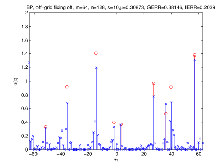
(a) BP

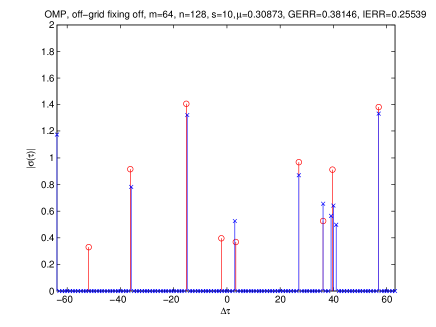
(b) OMP

(c) BPLOT

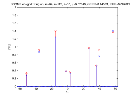
(d) SCOMP

Figure 1. Radar ranging (blue crosses) with $Q=1$ of off-grid targets (red circles) by (a) BP, (b) OMP with eq. (11) and (c) BPLOT, (d) SCOMP with eq. (20).

The idea of LOT is similar to that of the Band-excluded Locally Optimized Thresholding (BLOT) proposed in [12, 13] except without the band-exclusion step which is not needed here since the grid is well resolved. For brevity, we shall denote the combined algorithm of BP followed by LOT as BPLOT.

Successful recovery for OMP, SCOMP, BPLOT is defined as the recovery of target support to the grid accuracy, i.e. ${\hbox{\rm supp}}(\widehat{X})={\hbox{\rm supp}}(X)$. For BP, a recovery is counted as successful if ${\hbox{\rm supp}}(\widehat{X}^{s})={\hbox{\rm supp}}(X)$ where $\widehat{X}^{s}$ is the best $s$-sparse approximation of the BP recovery $\widehat{X}$ (i.e. thresholded BP). We distinguish two versions of thresholded BP: the grid-corrected version and the uncorrected version (“fixON BP” and “fixOff BP”, respectively, in the legend of Fig. 4, 8, 9(b) and 11(b)).

When recovery is successful, we measure the degree of success by the (relative) recovery error $\|X-\widehat{X}\|_{2}/\|X\|_{2}$ in the case of OMP, SCOMP, BPLOT and by $\|X-\widehat{X}^{s}\|_{2}/\|X\|_{2}$ in the case of BP. Note that for the system (20)

$$\|X-\widehat{X}\|_{2}/\|X\|_{2}=\sum_{k}\Big{|}{f_{\rm LC}(-k\Delta\tau-\xi_{k}\Delta\tau)\over f_{\rm LC}(-k\Delta\tau-\widehat{\xi}_{k}\Delta\tau)}e^{\pi iQ(\widehat{\xi}_{k}-\xi_{k})}\rho_{k}-\widehat{\rho}_{k}\Big{|}^{2}/\|\rho\|_{2}$$

while for the system (36) $\|X-\widehat{X}\|_{2}/\|X\|_{2}=\|\widehat{\rho}-\rho\|_{2}/\|\rho\|_{2}.$

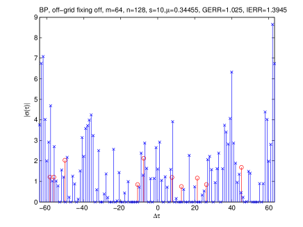
(a) BP

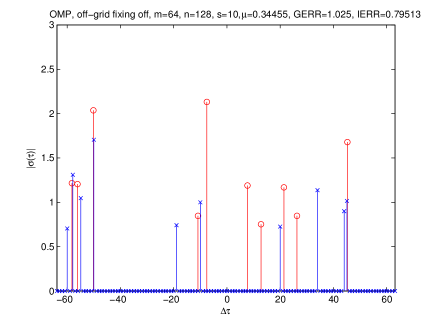
(b) OMP

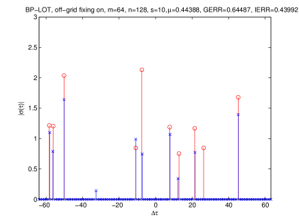
(c) BPLOT

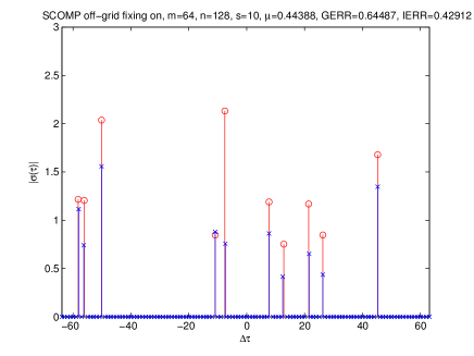
(d) SCOMP

Figure 2. Radar ranging with $Q=2$ by (a) BP, (b) OMP without grid correction and (c) BPLOT, (d) SCOMP with grid correction.

For radar ranging (13), we set the parameters $m=64,n=128$ and $Q=1,2$ (Fig.1-4). The gridding error for the formulation (11) is a whopping $38.1\%$ for $Q=1$ and $103\%$ for $Q=2$ while that for (20) is $14.5\%$ for $Q=1$ and 64.5% for $Q=2$ which still seem large. But surprisingly BPLOT (Fig.1(c)) and SCOMP (Fig.1(d) & 2(d)) can locate the targets to the grid accuracy, producing error of $8.8\%$ for Fig.1(c) & (d) and $43\%$ 2(d). Note that the second target from the right is missed by BPLOT in Fig.2(c). By contrast BP (Fig.1 (a) & 2 (a)) and OMP (Fig.1(b) & 2 (b)) poorly locate the targets for both $Q=1\&2$.

Fig.3 shows how the NLS technique can further improve the performance of SCOMP. The error for SCOMP-NLS is 2.2% and 31.2%, respectively, for $Q=1$ (Fig.3(a)) and $Q=2$ (Fig.3(b)). The worsening performance as $Q$ increases from 1 to 2 is probably due to the increasing gridding error.

Fig.4 shows the success rate computed out of 100 independent trials as a function of the target sparsity with the support recovery to the grid accuracy as the criterion for success. For each trial, the target support, amplitudes, time samples and external noise are independently chosen with the same sparsity.

For $Q=1$ (Fig.4(a)) BPLOT has the best performance while for $Q=2$ (Fig.4(b)) SCOMP is the best performer. Both BPLOT and SCOMP outperform both BP and OMP without grid correction.

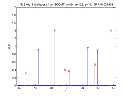
(a) SCOMP-NLS with $Q=1$

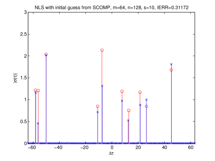
(b) SCOMP-NLS with $Q=2$

Figure 3. SCOMP-NLS produces ranging error of (a) $2.2\%$ with $Q=1$ and (b) $31.2\%$ with $Q=2$.

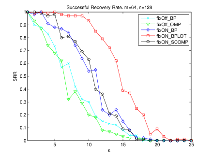
(a) $Q=1$

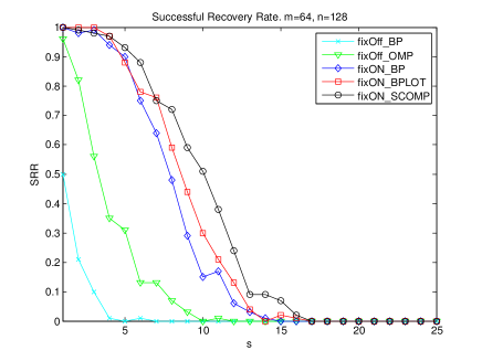
(b) $Q=2$

Figure 4. Success rate of ranging versus sparsity with (a) $Q=1$ and (b) $Q=2$. In the legend, “fixOff” means recovery without grid correction and “fixOn” means recovery with grid correction.

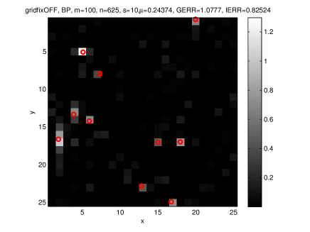
(a) BP

(b) OMP

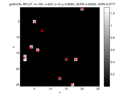
(c) BPLOT

(d) SCOMP

Figure 5. FDMF SAR imaging (white spots) of off-grid targets (red circles) with SAR scheme B and $Q=1$ by (a) BP, (b) OMP, both without grid correction, and (c) BPLOT, (d) SCOMP, both with grid correction.

For 2D Spotlight SAR in the FDMF regime, we use SAR schemes A & B (Sections 3) with $n=625,m=100,\nu_{0}=0,c_{0}=1$ (Fig.5-8). For $Q=1$, we set $\nu_{*}=1/\sqrt{2}$. For $Q=2$, we set $\nu_{*}=\sqrt{2}$. For SAR scheme A, we set $\phi=1/(2\pi),g=1/(\nu_{*}-\nu_{0})$ here and below.

First we consider the SAR scheme B. Fig.5 shows that only SCOMP locates the targets to the grid accuracy. Note that OMP and BPLOT miss the target located at around (15, 17) in (b) & (c), respectively. In Fig.6 with $Q=2$, BPLOT and SCOMP have the same results, locating the targets to the grid accuracy. The relative error is 45.7% for Fig.5(d) and 24.9% for Fig.6(d). After applying NLS to the SCOMP estimates, the error is reduced to 0.7% for $Q=1$ and 0.3% for $Q=2$ (Fig.7). This is a rate instance where the gridding and recovery errors are smaller with $Q=2$ than $Q=1$ and reminds us the subtle dependence of the gridding error on target and measurement configurations.

Fig.8 shows the success rate versus sparsity computed out of 100 independent trials. For both $Q=1$ and $Q=2$, SCOMP has the best performance. It is also clear from Fig.8, the results with $Q=1$ are better than those with $Q=2$ for all tested methods, despite the fact that the former’s bandwidth $1/\sqrt{2}$ is smaller than the latter’s $\sqrt{2}$.

Fig.9 shows the results of FDMF SAR ($m_{1}=m_{2}=10,\nu_{0}=0,\nu_{*}=1$) with the SAR scheme A which is easier to implement than the SAR scheme B (Section 3). The purpose is to compare the performance of the two sampling schemes. From Fig.8(a) and 9(b) we find that with the SAR scheme A, the performance of SCOMP worsens while the performances of grid-corrected thresholded BP and BPLOT improve. Note, however, that the bandwidth ($=1$) for Fig. 9(b) is larger than that ($=1/\sqrt{2}$) for Fig. 8(a).

For PDMF Spotlight SAR in Fig.10-11, we use the SAR scheme A with $n=625,m_{1}=m_{2}=14,\nu_{0}=1/2,\nu_{*}=1,c_{0}=1$, resulting in the fractional bandwidth $2/3$. Note that the total number of data $m=196$ almost doubles that for the FDMF case.

In Fig.10, only SCOMP manages to locate the targets to the grid accuracy (BPLOT misses the target located around (19, 22)), yielding an error of $49.9\%$. The error is reduced to 25.4% by NLS (Fig.11(a)). The success rate plot in Fig.11(b) shows that BPLOT and SCOMP have a similar, best performance, with the grid-corrected thresholded BP trailing closely behind.

From Fig.9(b) and 11(b), we find that grid-corrected thresholded BP, BPLOT and SCOMP have comparable performances with the SAR scheme A. Also, the similarity of the success rates (for grid-corrected thresholded BP, BPLOT and SCOMP) between Fig.9(b) and 11(b) indicates that increasing the spatial diversity and the number of data can compensate the deficiency in frequency diversity, up to a point.

For the purpose of comparison, Fig. 12 shows the results of PDMF SAR with (a) $m_{1}=28,m_{2}=7$ and (b) $m_{1}=7,m_{2}=28$, and other parameters the same as in Fig. 11. The number of degrees of diversity (=196) is the same for both Fig. 11 and 12. Clearly, the performances of grid-corrected thresholded BP, BPLOT and SCOMP improve (slightly) in Fig. 12(a) but degrade in Fig. 12(b) relative to Fig. 11(b). This means that, for a fixed bandwidth and number of degrees of diversity, there is an optimal distribution between the frequency diversity and the angular diversity. For example, for a smaller bandwidth, the frequency diversity should be decreased (and the angular diversity be increased) accordingly.

In the case of extreme deficiency in frequency diversity $(\nu_{*}-\nu_{0})/\nu_{0}\ll 1$, the gridding error dominates the data and our methods eventually break down.

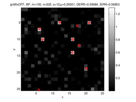
(a) BP

(b) OMP

(c) BPLOT

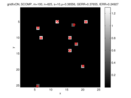
(d) SCOMP

Figure 6. FDMF SAR imaging with SAR scheme B and $Q=2$ by (a) BP, (b) OMP, without grid correction, and (c) BPLOT, (d) SCOMP, with grid correction.

(a) SCOMP-NLS with $Q=1$

(b) SCOMP-NLS with $Q=2$

Figure 7. SCOMP-NLS for FDMF SAR scheme B produces error of (a) $0.7\%$ with $Q=1$ and (b) $0.3\%$ with $Q=2$.

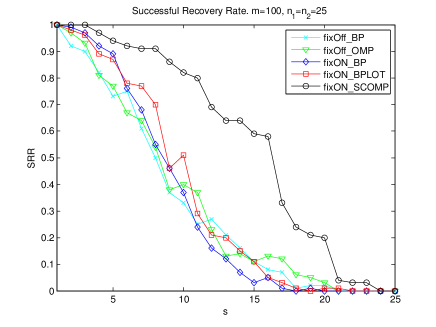
(a) $Q=1$

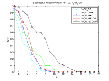
(b) $Q=2$

Figure 8. Success rate versus sparsity for FDMF SAR scheme B with (a) $Q=1$ and (b) $Q=2$. The legend is same as in Fig. 4.

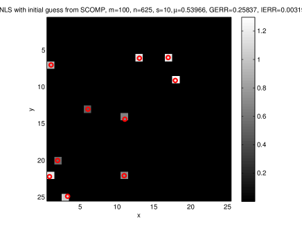
(a) SCOMP-NLS

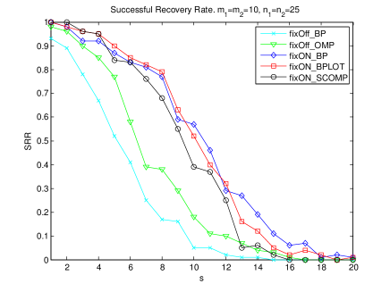
(b) Success rate vs. sparsity

Figure 9. FDMF SAR imaging with SAR scheme A ($m_{1}=m_{2}=10,\nu_{0}=0,\nu_{*}=1$). (a) SCOMP-NLS produces error of $0.3\%$. (b) Success rate versus sparsity. The legend is same as in Fig. 4.

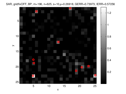
(a) BP

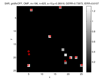
(b) OMP

(c) BPLOT

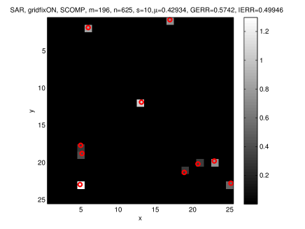
(d) SCOMP

Figure 10. PDMF SAR imaging with SAR scheme A by (a) BP, (b) OMP, without grid correction, and (c) BPLOT, (d) SCOMP, with grid correction.

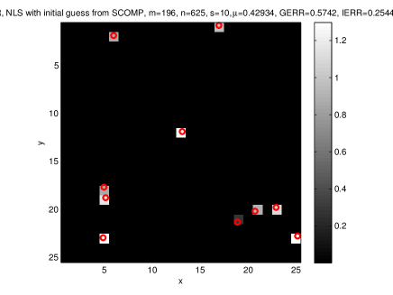
(a) SCOMP-NLS

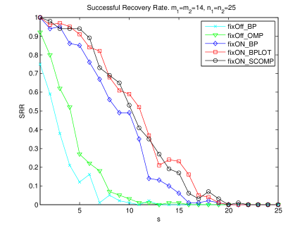
(b) Success rate versus sparsity

Figure 11. PDMF SAR imaging with scheme A ($m_{1}=m_{2}=14,\nu_{0}=1/2,\nu_{*}=1$). (a) SCOMP-NLS produces error of $25.4\%$. (b) Success rate versus sparsity. The legend is same as in Fig. 4.

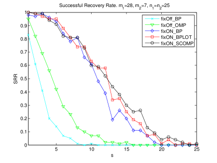
(a) $m_{1}=28,m_{2}=7$

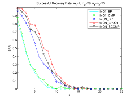
(b) $m_{1}=7,m_{2}=28$

Figure 12. Success rate of PDMF SAR scheme A with (a) $m_{1}=28,m_{2}=7$ (b) $m_{1}=7,m_{2}=28$. The legend is same as in Fig. 4.

5. Conclusion

We explored compressed sensing approach to monostatic radar with chirped signals or multi-frequency UNB waveforms. Particular attention is on the off-grid targets and the resulting intrinsically nonlinear gridding error.

We used the Taylor expansion of phase factor to approximate the signals from the off-grid targets and reduce the gridding error. We proposed a new algorithm, SCOMP, to solve the resulting grid-corrected system and gave a performance guarantee (Theorem 1). Our theory, however, does not fully account for the numerical performance of the proposed schemes, especially in the regime of low $Q$ which remains to be further analyzed (Remark 2).

In addition, we proposed technique (LOT) to enhance BP for the off-grid setting. The resulting method BPLOT can sometimes outperform SCOMP (Fig.4(a) and 9(b)). We extended SCOMP and the performance guarantee (Theorem 2) to Spotlight SAR and proposed the UNB multi-frequency version of implementation. Our numerical experiments show significant improvement over the standard CS methods, especially in locating sparse targets to the grid accuracy. The recovery of target amplitudes can be further improved by applying the nonlinear least squares with the SCOMP/BPLOT estimates as the initial guess.

Our numerical study indicates that in both radar ranging and SAR imaging, our methods perform best with $Q=1$. The latter corresponds to the setting where the grid spacing is around the resolution threshold of the probe, no more no less. Excessive bandwidth for the same grid spacing hinders the radar performance due to overall enhanced level of gridding error.

When full frequency diversity is not available, a good performance can be maintained up to about 2/3 fractional bandwidth. Further reduction in the probe bandwidth significantly degrades performance. Therefore the signals much be of ultra-wideband (UWB), defined as at least $1/4$ fractional bandwidth [22], if Spotlight SAR (29) is to be implemented with chirped signals and sparse measurements.

Implementing the proposed CS Spotlight SAR with multi-frequency UNB waveforms, instead of UWB pulses, has the added benefits of simpler transmitters, increased signal-to-noise ratio due to less unwanted thermal noise and increased signal-to-interference ratio due to avoiding the electromagnetic spectrum occupied by other civilian and military applications. The last of these benefits is a natural fit for the CS paradigm which opens the door for fully diversified, but sparse measurements in the frequency domains.

In the case of extreme deficiency in frequency diversity $(\nu_{*}-\nu_{0})/\nu_{0}\ll 1$, the gridding error dominates the data and our methods eventually break down. In this case SAR imaging of off-grid targets with sparse measurement requires a different approach than the proposed methods.

We plan to extend our methodology to the case of range-Doppler radar and SAR imaging of moving targets in the future.

Appendix A Proof of Lemma 1

Proof.

We prove the coherence bound for the matrix ${\mathbf{A}}=[{\mathbf{F}}\ {\mathbf{G}}]$.

The $k$-th column vector $A_{k}$ of ${\mathbf{A}}$ is given by

$$A_{jk}=\begin{cases}\mathrm{e}^{-2\pi\mathrm{i}Qk\bar{t}_{j}},&k\leq n\\ (\bar{t}_{j}-1/2)\mathrm{e}^{-2\pi\mathrm{i}Q(k-n)\bar{t}_{j}},&k>n.\end{cases}$$

Note that $\left\|{A_{k}}\right\|^{2}=m,k\leq n$ and $\mathbb{E}[\left\|{A_{k}}\right\|^{2}]={m}/{12},k>n.$ Consequently, the scalar product of two distinct columns of ${\mathbf{A}}$ has three possible forms:

$$b_{kk^{\prime}}=\sum_{j=1}^{m}a(\bar{t}_{j})\exp\left[{2\pi\mathrm{i}Q(k-k^{\prime})\bar{t}_{j}}\right]\ ,\quad a(t_{j})=1,\ (\bar{t}_{j}-1/2),\text{ or }\ (\bar{t}_{j}-1/2)^{2}\ ,$$

for $k,k^{\prime}=1,\ldots,n$. When $a(t_{j})=1$ or $(\bar{t}_{j}-1/2)^{2}$ both columns are drawn from ${\mathbf{F}}$ or ${\mathbf{G}}$ and thus $k\neq k^{\prime}$. When $a(t_{j})=\bar{t}_{j}-1/2$, one column is drawn from ${\mathbf{F}}$ and the other from ${\mathbf{G}}$. In the last case, $k$ and $k^{\prime}$ are arbitrary.

Let $S_{m}=\sum_{j=1}^{m}U_{j}$, $T_{m}=\sum_{j=1}^{m}V_{j}$ where

$$U_{j}=a(\bar{t}_{j})\cos\left[{2\pi Q(k-k^{\prime})\bar{t}_{j}}\right]\ ,\quad V_{j}=a(\bar{t}_{j})\sin\left[{2\pi Q(k-k^{\prime})\bar{t}_{j}}\right]$$

are independent (for different $j$) random variables in $[-1,1]$. We have

$$\left|{b_{kk^{\prime}}}\right| \leq\left|{b_{kk^{\prime}}-\mathbb{E}(b_{kk^{\prime}})}\right|+\left|{\mathbb{E}(b_{kk^{\prime}})}\right|$$

$$=\left|{S_{m}+\mathrm{i}T_{m}-\mathbb{E}S_{m}-\mathrm{i}\mathbb{E}T_{m}}\right|+\left|{\mathbb{E}(S_{m}+\mathrm{i}T_{m})}\right|.$$

Recall the Hoeffding inequality.

Proposition 2.

Let $U_{1},\ldots,U_{m}$ be independent random variables, and $S_{m}=\sum_{j=1}^{m}U_{j}$. Assume that $U_{j}\in[u,v]$, $j=1,2,\ldots,m$ almost surely, then we have

(47) $$\mathbb{P}(\left|{S_{m}-\mathbb{E}S_{m}}\right|\geq mt)\leq 2\exp\left[{-{2m^{2}t^{2}\over\sum_{j}(v-u)^{2}}}\right]$$

for all positive $t$.

Choosing $t=K/\sqrt{m}$ for some constant $K$, we have

$$\mathbb{P}(\left|{S_{m}-\mathbb{E}S_{m}}\right|\geq\sqrt{m}K)\leq 2\exp\left[{-K^{2}/2}\right].$$

Note that the quantities $S_{m}$ depend on $k-k^{\prime}$ but there are at most $n-1$ different values. The union bound yields

$$\mathbb{P}(\max_{k\neq k^{\prime}}\left|{S_{m}-\mathbb{E}S_{m}}\right|\geq\sqrt{m}K)\leq 2(n-1)\exp\left[{-K^{2}/2}\right],$$

and similarly

$$\mathbb{P}(\max_{k\neq k^{\prime}}\left|{T_{m}-\mathbb{E}T_{m}}\right|\geq\sqrt{m}K)\leq 2(n-1)\exp\left[{-K^{2}/2}\right].$$

We have

$$\mathbb{P}(\max_{k\neq k^{\prime}}\left|{b_{kk^{\prime}}-\mathbb{E}b_{kk^{\prime}}}\right|<\sqrt{2m}K)$$

$$=\quad \mathbb{P}(\max_{k\neq k^{\prime}}\left|{S_{m}+\mathrm{i}T_{m}-\mathbb{E}S_{m}-\mathrm{i}\mathbb{E}T_{m}}\right|<\sqrt{2m}K)$$

$$>\quad \Big{(}1-2(n-1)\exp\left[{-K^{2}/2}\right]\Big{)}^{2}\ >\ (1-\delta)^{2}$$

if $\delta>2n\exp\left[{-K^{2}/2}\right]$.

Now let us estimate the mean $\mathbb{E}(b_{kk^{\prime}})$ or $\mathbb{E}(S_{m}+\mathrm{i}T_{m})$ for $k\neq k^{\prime}$. Note that $\bar{t}_{j}$, $j=1,\ldots,m$, are independently and uniformly distributed in $[0,1]$. We have three different cases:

1. For $a(\bar{t}_{j})=1$,

   $$\mathbb{E}(b_{kk^{\prime}})=m\int_{0}^{1}\mathrm{e}^{2\pi\mathrm{i}Q(k-k^{\prime})t}\,\!\operatorname{d}\!t=0.$$

2. For $a(\bar{t}_{j})=\bar{t}_{j}-1/2$,

   $$\mathbb{E}(b_{kk^{\prime}})=m\int_{0}^{1}(t-1/2)\mathrm{e}^{2\pi\mathrm{i}Q(k-k^{\prime})t}\,\!\operatorname{d}\!t=m\mathrm{e}^{\pi iQ(k-k^{\prime})}\frac{(-1)^{(k-k^{\prime})Q}}{2\pi\mathrm{i}(k-k^{\prime})Q},\quad k\neq k^{\prime},$$

   and thus

   $$\left|{\mathbb{E}(b_{kk^{\prime}})}\right|\leq\frac{m}{2\pi Q},\quad k\neq k^{\prime}.$$

   On the other hand,

   $$\mathbb{E}(b_{kk})=m\int_{0}^{1}(t-1/2)\cdot 1\,\!\operatorname{d}\!t=0.$$

3. For $a(\bar{t}_{j})=(\bar{t}_{j}-1/2)^{2}$,

   $$\mathbb{E}(b_{kk^{\prime}})=m\int_{0}^{1}(t-1/2)^{2}\mathrm{e}^{2\pi\mathrm{i}Q(k-k^{\prime})t}\,\!\operatorname{d}\!t=m\mathrm{e}^{\pi iQ(k-k^{\prime})}\frac{(-1)^{(k-k^{\prime})Q}}{(2\pi(k-k^{\prime})Q)^{2}},\quad k\neq k^{\prime}$$

   and thus

   $$\left|{\mathbb{E}(b_{kk^{\prime}})}\right|\leq\frac{m}{(2\pi Q)^{2}}.$$

For $k,k^{\prime}\leq n$, since $\left\|{A_{k}}\right\|^{2}=m$,

(48) $$b_{kk^{\prime}}\leq\frac{C}{m}\sqrt{2m}K=C\frac{\sqrt{2}K}{\sqrt{m}},\quad k,k^{\prime}\leq n$$

for some universal constant $C$, with probability greater than $(1-\delta)^{2}$.

On the other hand, for $k>n$,

$$\|A_{k}\|^{2}_{2}=\sum_{j}(t_{j}-1/2)^{2}$$

which is a sum of $m$ i.i.d. random variables of mean $1/12$ on $[0,1/4]$. Applying Hoeffding inequality with $t={1/24}$, we have

$$\mathbb{P}\Big{(}|\|A_{k}\|^{2}_{2}-{m\over 12}|\geq{m\over 24}\Big{)}\leq 2e^{-{m/18}}$$

and thus

$$\mathbb{P}\Big{(}\|A_{k}\|^{2}_{2}\leq{m\over 24}\Big{)}\leq 2e^{-{m/18}}.$$

We conclude from these observations that

(49) $$b_{kk^{\prime}} \leq \frac{C}{m}\left[{\sqrt{2m}K+\frac{m}{2\pi Q}}\right]=C\cdot\left[{\frac{\sqrt{2}K}{\sqrt{m}}+\frac{1}{2\pi Q}}\right],\quad k\leq n<k^{\prime}$$

(50) $$b_{kk^{\prime}} \leq \frac{C}{m}\left[{\sqrt{2m}K+\frac{m}{(2\pi Q)^{2}}}\right]=C\cdot\left[{\frac{\sqrt{2}K}{\sqrt{m}}+\frac{1}{(2\pi Q)^{2}}}\right],\quad k,k^{\prime}>n$$

with probability at least $(1-\delta)^{2}-4e^{-m/18}$. (48)-(50) are what we set out to prove.

∎

Appendix B Proof of Theorem 1

Proof.

We prove the theorem by induction. Without loss of generality, we assume that the columns of ${\mathbf{A}}$ have unit 2-norm.

In the first step,

$$|F^{*}_{J_{1}}Y|+|G^{*}_{J_{1}}Y| = |X_{J_{1}}F^{*}_{J_{1}}F_{J_{1}}+X_{J_{2}}F_{J_{1}}^{*}F_{J_{2}}+...+X_{J_{s}}F_{J_{1}}^{*}F_{J_{s}}+$$

$$X^{\prime}_{J_{1}}F^{*}_{J_{1}}G_{J_{1}}+X^{\prime}_{J_{2}}F_{J_{1}}^{*}G_{J_{2}}+...+X^{\prime}_{J_{s}}F_{J_{1}}^{*}G_{J_{s}}+F_{J_{1}}^{*}E|$$

$$+|X^{\prime}_{J_{1}}G^{*}_{J_{1}}G_{J_{1}}+X^{\prime}_{J_{2}}G_{J_{1}}^{*}G_{J_{2}}+...+X^{\prime}_{J_{s}}G_{J_{1}}^{*}G_{J_{s}}+$$

$$X_{J_{1}}G^{*}_{J_{1}}F_{J_{1}}+X_{J_{2}}G_{J_{1}}^{*}F_{J_{2}}+...+X_{J_{s}}G_{J_{1}}^{*}F_{J_{s}}+G_{J_{1}}^{*}E|$$

$$\geq X_{\rm max}-X_{\rm max}(2s-1)\mu-2\|E\|_{2}.$$

On the other hand, $\forall l\notin\hbox{supp}(X)$,

$$|F^{*}_{l}Y|+|G^{*}_{l}Y| = |X_{J_{1}}F^{*}_{l}F_{J_{1}}+X_{J_{2}}F_{l}^{*}F_{J_{2}}+...+X_{J_{s}}F_{l}^{*}F_{J_{s}}+$$

$$X^{\prime}_{J_{1}}F^{*}_{l}G_{J_{1}}+X^{\prime}_{J_{2}}F_{l}^{*}G_{J_{2}}+...+X^{\prime}_{J_{s}}F_{l}^{*}G_{J_{s}}+F_{l}^{*}E|$$

$$+|X^{\prime}_{J_{1}}G^{*}_{l}G_{J_{1}}+X^{\prime}_{J_{2}}G_{l}^{*}G_{J_{2}}+...+X^{\prime}_{J_{s}}G_{l}^{*}G_{J_{s}}+$$

$$X_{J_{1}}G^{*}_{l}F_{J_{1}}+X_{J_{2}}G_{l}^{*}F_{J_{2}}+...+X_{J_{s}}G_{l}^{*}F_{J_{s}}+G_{l}^{*}E|$$

$$\leq 2X_{\rm max}s\mu+2\|E\|_{2}.$$

Hence, if

$$(4s-1)\mu+\frac{4\|E\|_{2}}{X_{\rm max}}<1,$$

then the right hand side of (B) is greater than the right hand side of (B) which implies that the first index selected by OMP must belong to $\hbox{supp}(X)$.

To continue the induction process, we need the following result.

Proposition 3.

Let $Y={\mathbf{F}}X+{\mathbf{G}}X^{\prime}+E$ where ${\hbox{\rm supp}}(X^{\prime})\subseteq{\hbox{\rm supp}}(X)={\mathcal{S}}$. Let ${\mathcal{S}}^{k}$ be a set of $k$ indices containing both ${\hbox{\rm supp}}{(\widehat{X})}$ and ${\hbox{\rm supp}}(\widehat{X}^{\prime})$. Define

(53) $$Y^{\prime}=Y-{\mathbf{F}}\widehat{X}-{\mathbf{G}}\widehat{X}^{\prime}.$$

Clearly, $Y^{\prime}={\mathbf{F}}(X-\widehat{X})+{\mathbf{G}}(X^{\prime}-\widehat{X}^{\prime})+E$. If ${\mathcal{S}}^{k}\subseteq{\mathcal{S}}$ and the sparsity $s$ of $X$ satisfies $4s<1+1/\mu$, then ${\mathbf{F}}(X-\widehat{X})+{\mathbf{G}}(X^{\prime}-\widehat{X}^{\prime})$ has a unique sparsest representation ${\mathbf{F}}Z+{\mathbf{G}}Z^{\prime}$ with $Z=X-\widehat{X}$ and $Z^{\prime}=X^{\prime}-\widehat{X}^{\prime}$.

Proof.

Clearly ${\hbox{\rm supp}}(Z),{\hbox{\rm supp}}(Z^{\prime})\subseteq{\hbox{\rm supp}}(X)$. Since

$$\|Z\|_{0}+\|Z^{\prime}\|_{0}\leq 2s<{1\over 2}(1+{1\over\mu})$$

we conclude that $Z$ and $Z^{\prime}$ are the unique sparsest representation of ${\mathbf{F}}(X-\widehat{X})+{\mathbf{G}}(X^{\prime}-\widehat{X}^{\prime})$. ∎

Proposition 3 says that selection of a column, followed by the formation of the residual signal, leads to a situation like before, where the ideal noiseless signal has no more representing columns than before, and the noise level is the same.

Suppose that the set ${\mathcal{S}}^{k}\subseteq{\hbox{\rm supp}}(X)$ of $k$ distinct indices has been selected and that $\widehat{X}$ in Proposition 3 solves the following least squares problem

(54) $$\left(\begin{matrix}\widehat{X}\\ \widehat{X}^{\prime}\end{matrix}\right)=\hbox{arg}\min\|Y-[{\mathbf{F}}\ {\mathbf{G}}]Z\|_{2},\quad\hbox{s.t.}\quad{\hbox{\rm supp}}(Z)\subseteq{\mathcal{S}}^{k}.$$

Let ${\mathbf{F}}_{{\mathcal{S}}^{k}}$ and ${\mathbf{G}}_{{\mathcal{S}}_{k}}$ be, respectively, the column submatrices of ${\mathbf{F}}$ and ${\mathbf{G}}$ indexed by the set ${\mathcal{S}}^{k}$. By (53) and (54), ${\mathbf{F}}^{*}_{{\mathcal{S}}^{k}}Y^{\prime}={\mathbf{G}}^{*}_{{\mathcal{S}}_{k}}Y^{\prime}=0,$ which implies that no element of ${\mathcal{S}}^{k}$ gets selected at the $(k+1)$-st step.

In order to ensure that some element in ${\hbox{\rm supp}}(X)\setminus{\mathcal{S}}^{k}$ gets selected at the $(k+1)$-st step we only need to repeat the calculation (B)-(B) to obtain the condition

$$(4s-1)\mu+\frac{4\|E\|_{2}}{|X_{J_{k+1}}|+|X^{\prime}_{J_{k+1}}|}<1$$

which follows from

(55) $$(4s-1)\mu+\frac{4\epsilon}{X_{\rm min}}<1.$$

By the $s$-th step, all elements of the support set are selected and by the nature of the least squares solution the $2$-norm of the residual is at most $\epsilon$. Thus the stopping criterion is met and the iteration stops after $s$ steps.

On the other hand, it follows from the calculation

$$2\|Y^{\prime}\|_{2} \geq \big{|}F^{*}_{J_{k+1}}Y^{\prime}\big{|}+\big{|}G^{*}_{J_{k+1}}Y^{\prime}\big{|}$$

$$= |X_{J_{k+1}}+\sum_{i=k+2}^{s}X_{J_{i}}F_{J_{k+1}}^{*}F_{J_{i}}+\sum_{i=k+1}^{s}X^{\prime}_{J_{i}}F_{J_{k+1}}^{*}G_{J_{i}}+F_{J_{k+1}}^{*}E|$$

$$+ |X^{\prime}_{J_{k+1}}+\sum_{i=k+1}^{s}X_{J_{i}}G_{J_{k+1}}^{*}F_{J_{i}}+\sum_{i=k+2}^{s}X^{\prime}_{J_{i}}G_{J_{k+1}}^{*}G_{J_{i}}+G_{J_{k+1}}^{*}E|$$

$$\geq |X_{J_{k+1}}|+|X^{\prime}_{J_{k+1}}|-(|X_{J_{k+1}}|+|X^{\prime}_{J_{k+1}}|)\mu$$

$$-2(s-k-1)\mu(|X_{J_{k+2}}|+|X_{J_{k+2}}|)-2\|E\|_{2}$$

$$\geq (1-\mu(2s-2k-1))(|X_{J_{k+1}}|+|X^{\prime}_{J_{k+1}}|)-2\|E\|_{2}$$

and (55) that $\|Y^{\prime}\|_{2}>\epsilon$ for $k=0,1,\cdots,s-1$. Thus the iteration does not stop until $k=s$.

By (54), we have

$$\|Y-{\mathbf{F}}\widehat{X}-{\mathbf{G}}\widehat{X}^{\prime}\|_{2}\leq\|Y-{\mathbf{F}}X-{\mathbf{G}}X^{\prime}\|_{2}\leq\epsilon$$

and

$$\|{\mathbf{F}}(X-\widehat{X})+{\mathbf{G}}(X^{\prime}-\widehat{X}^{\prime})\|^{2}_{2}\leq 2\|Y-{\mathbf{F}}X-{\mathbf{G}}X^{\prime}\|^{2}_{2}+2\|Y-{\mathbf{F}}\widehat{X}-{\mathbf{G}}\widehat{X}^{\prime}\|^{2}_{2}\leq 2\epsilon^{2}$$

implying that

$$\|\widehat{X}-X\|^{2}_{2}+\|\widehat{X}^{\prime}-X^{\prime}\|_{2}^{2}\leq 2\epsilon^{2}/\lambda^{2}_{\rm min}$$

where

$$\lambda_{\rm min}=\hbox{\rm the $2s$-th largest singular value of ${\mathbf{A}}$.}$$

.

The desired error bound can now be obtained from the following result (Lemma 2.2, [6]).

Proposition 4.

Suppose $2s<1+\mu^{-1}$. Every $m\times(2s)$ column submatrix of ${\mathbf{A}}$ has the $2s$-th singular value bounded below by $\sqrt{1-\mu(2s-1)}$.

By Proposition 4, $\lambda_{\rm min}\geq\sqrt{1-\mu(2s-1)}$ and thus the desired estimate (27) follows. ∎

Acknowledgement. We thank an anonymous referee for a suggestion that inspired our formulation of Algorithm 3 (LOT) in Section 6. The research is partially supported by the NSF grant DMS-0908535.

References

• [1] R. Baraniuk and P. Steeghs, “Compressive radar imaging.” IEEE Radar Conf. (2007), 128-133.
• [2] E. J. Candès, “The restricted isometry property and its implications for compressed sensing.” Comptes Rendus Mathematique 346 (2008), 589-592.
• [3] E.J. Candès, Y.C. Eldar, D. Needell, and P. Randall, “Compressed sensing with coherent and redundant dictionaries,” Appl. Comput. Harmon. Anal., 31 (2011), pp. 59 73.
• [4] M. Cheney and B. Borden, “Imaging moving targets from scattered waves.” Inverse Probl. 24 (2008), 035005.
• [5] Y. Chi, L. L. Scharf, A. Pezeshki and A. R. Calderbank, “Sensitivity to basis mismatch in compressed sensing.” IEEE T. Signal Proces. 59 (2011), 2182-2195.
• [6] D.L. Donoho, M. Elad and V.N. Temlyakov, “Stable recovery of sparse overcomplete representations in the presence of noise,” IEEE Trans. Inform. Theory 52 (2006) 6-18.
• [7] M.F. Duarte and R.G. Baraniuk, “Spectral compressive sensing,” Appl. Comput. Harmon. Anal., 32 (2012).
• [8] J. Ender, “On compressive sensing applied to radar.” Signal Proces. 90 (2010), 1402-1414.
• [9] A. Fannjiang, “Compressive inverse scattering I. High-frequency SIMO/MISO and MIMO measurements.” Inverse Probl. 26 (2010), 035008.
• [10] A. Fannjiang, “Compressive inverse scattering II. Multi-shot SISO measurements with Born scatterers.” Inverse Probl. 26 (2010), 035009.
• [11] A. Fannjiang and W. Liao, “Mismatch and resolution in compressive imaging,” Wavelets and Sparsity XIV, edited by Manos Papadakis, Dimitri Van De Ville, Vivek K. Goyal, Proc. SPIE Vol. 8138, 0Y1-9,2011.
• [12] A. Fannjiang and W. Liao, “Coherence-Pattern guided compressive sensing with unresolved grids,” SIAM J. Imag. Sci. 5 (2012), 179-202.
• [13] A. Fannjiang and W. Liao, “Super-resolution by compressive sensing algorithms,” IEEE Proc. Asilomar conference on signals, systems and computers, 2012.
• [14] M. J. Gerry, L. C. Potter, I. J. Gupta, and A. van der Merwe, “A parametric model for synthetic aperture radar measurements,” IEEE Trans. Antennas Propag. 47, pp. 1179 1188, 1999.
• [15] M. Herman and T. Strohmer, “High resolution radar via compressed sensing.” IEEE Trans. Signal Process. 57 (2009), 2275-2284.
• [16] M. Herman and T. Strohmer, “General deviants: an analysis of perturbations in compressed sensing,” IEEE J. Sel. Topics Signal Process. 4 (2010), pp. 342 - 349.
• [17] C. V. Jakowatz et al., Spotlight-Mode Synthetic Aperture Radar: A Signal Processing Approach. New York: Springer, 1996.
• [18] J. B. Keller, “Geometrical theory of diffraction”, J. Opt. Soc. Amer., 5 (1962) pp. 116 130.
• [19] D. C. Munson, Jr., J. D. O’Brien, and W. K. Jenkins, “A tomographic formulation of spotlight-mode synthetic aperture radar,” Proc. IEEE 71, pp. 917-925, 1983.
• [20] L. C. Potter, E. Ertin, J. T. Parker and Müjdat Çetin, “Sparsity and compressed sensing in radar imaging.” Proc. IEEE 98 (2010), 1006-1020.
• [21] H. Rauhut, “Stability results for random sampling of sparse trigonometric polynomials.” IEEE Trans. Inform. Theory 54 (2008), 5661-5670.
• [22] J. D. Taylor, Introduction to Ultra-wideband Radar Systems, CRC Press, Boca Raton, 1995.
• [23] J. Yang and Y. Zhang, “Alternating direction algorithms for L1 problems in compressive sensing,” SIAM J. Sci. Comput. 33 (2011), 250 - 278.
• [24] H. Zhu, G. Leus and G. B. Giannakis, “Sparsity-cognizant total least-squares for perturbed compressive sampling,” IEEE Trans. Sign. Process. 59 (2011), 2002-2016.