Instrumental and Observational Artifacts in Quiet Sun Magnetic Flux Cancellation Functions

Abstract

Under the assumption that the photospheric quiet-Sun magnetic field is turbulent, the cancellation function has previously been used to estimate the true, resolution-independent mean, unsigned vertical flux $\langle|B_{z}|\rangle_{\mathrm{true}}$. We show that the presence of network elements, noise, and seeing complicate the measurement of accurate cancellation functions and their power-law exponents $\kappa$. Failure to exclude network elements previously led to too low estimates of both the cancellation exponent $\kappa$ and of $\langle|B_{z}|\rangle_{\mathrm{true}}$. However, both $\kappa$ and $\langle|B_{z}|\rangle_{\mathrm{true}}$ are over-estimated due to noise in magnetograms. While no conclusive value can be derived with data from current instruments, our Hinode/SP results of $\kappa\lessapprox 0.38$ and $\langle|B_{z}|\rangle_{\mathrm{true}}\lessapprox 270\,$gauss can be taken as upper bounds.

1 Introduction

Turbulent fields possess self-similar power-laws, i.e., they are fractals [Brandenburg et al. (1992), Frisch (1995)]. Such power-laws (i.e, self-similarity) are found in systems where the underlying physical processes are the same at all scales (e.g., vortex or flux tube stretching suggested by F95). In these systems, the fields have the same degree of complexity (look the same) regardless of the observational resolution. For example, incompressible magnetohydrodynamics (MHD) is expected [Iroshnikov (1964), Kraichnan (1965), Goldreich and Sridhar (1995)] and found (e.g., LeBrPo+2009; PiGrMiPo2011) to display self-similar magnetic energy spectra. Power-law magnetic energy spectra are also seen in compressible, stratified MHD photospheric simulations [Brandenburg (1995)] including those with realistic radiation and partial ionization [Pietarila Graham, Cameron, and Schüssler (2010), Moll et al. (2011)]. Power-laws are found in solar observations of the line-of-sight magnetic energy, kinetic energy, and even the granulation intensity [Abramenko and Yurchyshyn (2010a), Abramenko and Yurchyshyn (2010b), Goode et al. (2010)]. Power-laws are, of course, fundamental in measurements of the fractal dimension of magnetic structures in both observations and simulations (e.g., JaVoKn2003). Both the observations and simulations above indicate that the quiet Sun magnetic field is likely turbulent.

The application of turbulent self-similarity to estimate the true mean unsigned vertical flux from magnetograms was introduced by Pietarila Graham, Danilovic, and Schüssler (2009, hereafter PGDS2009). Define the “net” flux ($\mathrm{Flux}_{l}$) at scale $l$ for any vertical field $f_{z}$ to be the flux remaining after averaging over boxes $\mathcal{A}_{i}(l)$ of edge length $l$:

$$\mathrm{Flux}_{l}=\sum_{i}\bigg{|}\int_{\mathcal{A}_{i}(l)\in\mathcal{A}}f_{z}\mathrm{d}a\bigg{|}\,,\ilabel{eq:netflux}$$ (1)

where the boxes partition the total area: $\bigcup_{i}\mathcal{A}_{i}(l)=\mathcal{A}$. The unsigned flux of the field is given by

$$\mathrm{Flux}_{0}=\int_{\mathcal{A}}|f_{z}|\mathrm{d}a\,.\ilabel{eq:netflux}$$ (2)

The ratio of the net flux at length scale $l$ to the true mean unsigned flux (i.e., flux cancellation) is called the partition function

$$\chi(l)=\frac{\mathrm{Flux}_{l}}{\mathrm{Flux}_{0}}\,,\ilabel{eq:partition}$$ (3)

which follows a power-law for self-similar fields,

$$\chi(l)\propto l^{-\kappa}\,,\ilabel{eq:kappa}$$ (4)

where $\kappa$ is the cancellation exponent Ott et al. (1992). For a completely self-similar field, knowledge of net flux at any scale and of the power-law scaling exponent implies knowledge of net flux at all scales and, hence, the unsigned flux. The two extreme examples are a unipolar field, for which the net flux always equals the unsigned flux ($\kappa=0$), and a random field. For a random field, the observed net flux equals the unsigned flux times the ratio of the noise correlation length to the diameter of the resolution element ($\kappa=1$). See the Appendix for a mathematical derivation of the random noise case and of the general formula, Equation (eq:extrapolate), to determine the unsigned flux for a completely self-similar field given $\kappa$ and the correlation length below which the field becomes smooth.

Under the assumption that the quiet-Sun magnetic field is turbulent, the theoretical framework in the Appendix applies. This might suggest that the unsigned quiet-Sun flux could be deduced from Zeeman-based instruments. Such studies have previously been made (PGDS2009; St2011). PGDS2009 observed a power-law in $\chi(l)$ (which they dubbed the “cancellation function” when applied to a magnetogram) down to $\approx 200\,$km with $\kappa=0.26$ in Hinode Spectro-Polarimeter (SP; HinodeSOT) data. Note that power-laws for $\chi(l)$ have previously been seen in simulations of the electric currents Sorriso-Valvo et al. (2002); Pietarila Graham, Mininni, and Pouquet (2005) and in solar observations of current-helicity Sorriso-Valvo et al. (2003); Abramenko (2003); Sorriso-Valvo et al. (2004); Abramenko and Yurchyshyn (2010a). PGDS2009 used Equation (eq:extrapolate) to estimate the net flux at a scale of $800\,$m to be $\approx 50\,$G. Turbulent power-laws (e.g., energy spectra and $\chi(l)$) extend only down to the dissipative range, but the magnetic diffusion scale is expected to be significantly smaller than $800\,$m. Thus, the extrapolation was taken as a lower bound, $\mathrm{Flux}_{0}>50\,$G (gauss). This result was found to be in agreement with a separate extrapolation from radiative MHD simulations.

Other estimates of $\kappa$ can be made. LiKuSoNa+2008 found a 30% increase in flux changing from a resolution of 1^′′ to 0.33^′′ which indicates $\kappa=0.24$. SoBaDa+2010 found a factor of 3.7 more flux on doubling of resolution, indicating $\kappa=1.9$. Using many instruments with different spatial resolutions, SaAlMaGo2011 fit $\mathrm{Flux}_{l}\propto l^{-1}$, i.e., $\kappa$=1. The data set used by PGDS2009 was recalibrated by St2011 leading to more pronounced high field strength tails in the flux probability distribution. The power law from the recalibrated magnetogram yielded a value of $\kappa$ that is half of the value derived by PGDS2009. In addition to the SP magnetogram St2011 computed cancellation functions from a set of Hinode Narrow-band Filter Imager (NFI) Na i $D_{1}$ magnetograms. The resulting $\kappa$ was found to be 0.127, i.e., very similar to the value for the recalibrated SP magnetogram. In order to agree with Hanle-based magnetic field measurements, this cancellation function needs to be extrapolated down to a spatial scale of 10 – 100 m.

Another application for using the fractal nature of magnetic fields is in flare predictions. Previous works (SoVaAbCa+2003b, 2004; AbYu2010) have shown it to be promising. However, as in the case of cancellation functions, the data-sample sizes used to study the suitability of the method have been limited. Recently Georgoulis2011 has shown how previous analyses may have been misleading: A statistical comparison of flaring and non-flaring active regions found that the fractal properties of the line-of-sight magnetic field cannot distinguish flaring and non-flaring active regions. Many of the previous works, however, used current helicity, not magnetic flux, for the analysis and therefore the conclusions of Georgoulis2011 may not apply to them.

Prompted by the results of PGDS2009, St2011, and Georgoulis2011, we suggest that measurements of the cancellation function do not confront the reality of the observational data. Such confrontation is the aim of this paper. We analyze the statistics of quiet Sun cancellation functions using magnetograms from three different instruments. We test if the cancellation exponent $\kappa$ is robust within and among the instruments to point out observational artifacts in the measurement of $\kappa$ and to determine if any conclusive values or bounds can be made with existing data.

2 Data and Methods

We use altogether $\approx$800 magnetograms from the Helioseismic and Magnetic Imager (HMI; HMI) on the Solar Dynamics Observatory (SDO) satellite, Michelson Doppler Imager (MDI; MDI) on the Solar and Heliospheric Observatory (SOHO) sarellite, and Hinode SP. The largest data set, 700 HMI magnetograms, allows us to characterize the variation within a single instrument. Data from MDI and SP allow for inter-instrument comparisons and for identification of possible instrumental artifacts as well as for determination of the effects of spatial resolution and magnetogram noise.

The HMI data consist of daily (from end of March 2010 to mid-June 2011) 4 s integration magnetograms taken around 12:00 UT. We analyze a $501\times 501$ pixel ($\approx 253$ ^′′$\times 253$ ^′′) area around the disk center. For MDI, we use $301\times 301$ pixel ($\approx 182$ ^′′$\times 182$ ^′′) sub-regions, excluding active regions, in high resolution magnetograms (level 1.8) near the solar disk center. Note that a calibration coefficient (BSCALE=2.81) is applied to the MDI magnetograms to convert from counts to gauss leading to the magnetograms being quantized in units of BSCALE.

The SP magnetograms are the longitudinal magnetic field measurements in Level 1D data with exposure times varying between 1.6 and 12 s. Both $\approx$0.16^′′ and $\approx$0.32^′′ pixel size magnetograms are included in the data set. We choose observations of quiet Sun taken near the disk center. The size of SP magnetograms ranges from $\approx$ $400\times 400$ to $1000\times 1000$ pixels ($\approx 64$ ^′′$\times 64$ ^′′–160 ^′′$\times 160$ ^′′).

Cancellation functions [$\chi(l)$] are computed for each magnetogram using the Monte Carlo technique of CaLaRu+1994. Linear fits to $\chi(l)$ in log-log space are made for three different spatial scales: small scale $<$2^′′  (exponent $\kappa_{\mathrm{S}}$), intermediate scale 2 – 5^′′ ($\kappa_{\mathrm{I}}$) and large scale 2 – 9 ^′′ ($\kappa_{\mathrm{L}}$). While the physical scales are the same for all instruments, the number of pixels for fitting the exponent varies due to the instruments’ different pixel sizes (HMI $\approx$0.5^′′, MDI $\approx$0.6^′′, SP $\approx$0.16^′′or $\approx$0.32^′′). The spatial scales were chosen to be sensitive to the scales most affected by noise ($\kappa_{\mathrm{S}}$) and scales not dominated by noise, but still below the spatial scale of the network ($\kappa_{\mathrm{I}}$ and $\kappa_{\mathrm{L}}$). The overlap of $\kappa_{\mathrm{I}}$ and $\kappa_{\mathrm{L}}$ ensures that enough data points (14 for HMI, 11 for MDI and 24 or 47, depending on pixel size, for SP) are included in fitting $\kappa_{\mathrm{L}}$ and that the results are not strongly sensitive to the upper cut-off (5^′′ or 9^′′) of the fitted spatial scales.

Additionally, the mean unsigned flux $\langle|B_{z}|\rangle$ and flux imbalance $\langle B_{z}\rangle$/$\langle|B_{z}|\rangle$ are computed for each magnetogram.

3 Results

3.1 Exponents and Effects of Network

The results of the analysis on the HMI cancellation function are summarized in Figure fig:hmi-all and Table table:hmi-mdi. Compared to large spatial scales ($>$10^′′, for which we do not fit a power-law), the exponents at the smaller scales are fairly similar: $\kappa_{\mathrm{I}}$ and $\kappa_{\mathrm{L}}$are nearly identical, which indicates that we are fitting a genuine power-law at these scales ( 2^′′to 9^′′). $\chi(l)$ turns up at the small scales as is demonstrated by $\kappa_{\mathrm{S}}$ having $\approx$30% higher values than $\kappa_{\mathrm{I}}$ and $\kappa_{\mathrm{L}}$. The increase is partially due to contributions from noise becoming more dominant (see Section sec:noise and note that $\kappa_{\mathrm{noise}}=1$; SVCN+02 and the Appendix). Note that there is both scatter (standard deviation up to 6% of the mean) and systematic differences between the exponents of power-law fit to different magnetograms.

All exponents decrease as a function of $\langle|B_{z}|\rangle$, $\langle|B_{z}|\rangle$$\equiv\mathrm{Flux}_{l}$ for $l=1\,$pixel. The more flux there is in the magnetogram, the smaller each $\kappa$ is. A linear fit of $\kappa$ as a function of $\log$$\langle|B_{z}|\rangle$ shows that the decrease is strongest for $\kappa_{\mathrm{L}}$ and weakest for $\kappa_{\mathrm{S}}$. No correlation is found for $\kappa$ and the global (full-disk) unsigned flux, which reflects the overall activity present on the solar disk at a given time: The cancellation functions reflect the local magnetic environment, whose fractal properties do not appear to be influenced by the global field. $\kappa$ does not depend on the flux imbalance at small imbalances (below $\approx$10%). For imbalances greater than $\approx$10% $\kappa$ decreases with increasing imbalance on all spatial scales.

The exponents show no strong temporal evolution or indications of the exponent changing as solar activity increases (Figure fig:hmi-ts). Since the activity in the rising phase of the solar cycle emerges at high latitudes, it is not surprising that no significant change in the exponent is seen near disk center.

The results for MDI are shown in Figure fig:mdi-all and Table table:hmi-mdi. They are qualitatively similar to HMI, confirming that the trends ($\langle|B_{z}|\rangle$, flux imbalance) are of solar, not instrumental, origin. The exponents are larger and have more scatter (standard deviation is 9% of the mean). Also the dependence of $\kappa$ on $\langle|B_{z}|\rangle$ is stronger.

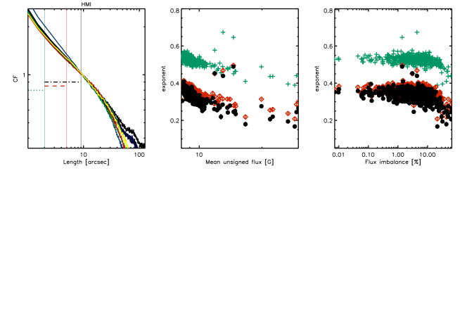
Figure 1.: HMI cancellation functions. Left: Cancellation functions for selected magnetograms (in various colors) normalized to unity at 9^′′. Vertical and horizontal lines mark ranges used for fitting the exponents ($\kappa_{\mathrm{S}}$ in green dotted line and crosses, $\kappa_{\mathrm{I}}$ in red dashed line and diamonds, and $\kappa_{\mathrm{L}}$ in black dash-dotted line and circles). The same colors and symbols are used in all plots to differentiate between the spatial scales. Middle: Cancellation exponents as a function of $\langle|B_{z}|\rangle$. Error bars show 1$\sigma_{\mathrm{fit}}$. Right: Exponents as a function of flux imbalance. fig:hmi-all

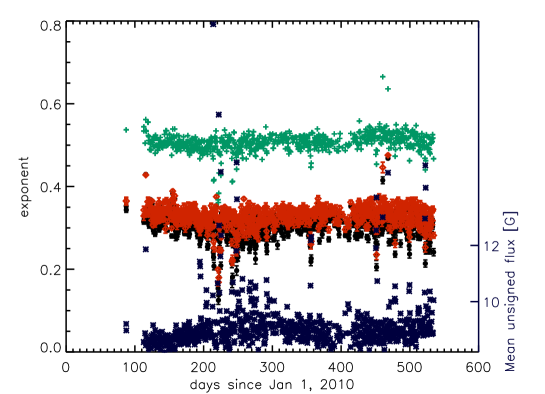
Figure 2.: HMI cancellation exponents as a function of time. $\kappa_{\mathrm{S}}$ is shown in green crosses, $\kappa_{\mathrm{I}}$ in red diamonds, and $\kappa_{\mathrm{L}}$ in black circles. $\langle|B_{z}|\rangle$is shown in dark blue $\ast$ (y-axis on right). fig:hmi-ts

Figure 3.: MDI cancellation functions. Left: Cancellation functions for selected magnetograms (in various colors) normalized to unity at 9^′′. Vertical and horizontal lines mark ranges used for fitting the exponents ($\kappa_{\mathrm{S}}$ in green dotted line and crosses, $\kappa_{\mathrm{I}}$ in red dashed line and diamonds, and $\kappa_{\mathrm{L}}$ in black dash-dotted line and circles). The same colors and symbols are used in all plots to differentiate between the scales. Middle: Cancellation exponents as a function of $\langle|B_{z}|\rangle$. Error bars show 1$\sigma_{\mathrm{fit}}$. Right: Exponents as a function of flux imbalance.fig:mdi-all

Table 1.: Power-law fits to $\chi(l)$ for HMI, MDI, and SP magnetograms.table:hmi-mdi

table:sp Mean Standard deviation c f¹ HMI $\kappa_{\mathrm{S}}$ 0.53 0.017 0.74 (0.01) -0.22 (0.01) $\kappa_{\mathrm{I}}$ 0.36 0.020 0.61 (0.01) -0.26 (0.01) $\kappa_{\mathrm{L}}$ 0.35 0.022 0.66 (0.01) -0.34 (0.01) MDI² $\kappa_{\mathrm{S}}$ 0.61 0.053 1.62 (0.06) -0.64 (0.03) $\kappa_{\mathrm{I}}$ 0.45 0.033 1.47 (0.07) -0.65 (0.04) $\kappa_{\mathrm{L}}$ 0.42 0.036 1.51 (0.08) -0.70 (0.05) SP $t_{\mathrm{exp}}<$2 s $\kappa_{\mathrm{S}}$ 0.30 0.020 – – $\kappa_{\mathrm{I}}$ 0.28 0.020 – – $\kappa_{\mathrm{L}}$ 0.29 0.014 – – $t_{\mathrm{exp}}>$2 s $\kappa_{\mathrm{S}}$ 0.24 0.0063 – – $\kappa_{\mathrm{I}}$ 0.26 0.014 – – $\kappa_{\mathrm{L}}$ 0.28 0.032 – –
${}^{\mathrm{1}}\kappa=c$+$f$*$\log$($\langle|B_{z}|\rangle$) $\sigma_{\mathrm{fit}}$ is given in parentheses.
²Only magnetograms with flux imbalances below 5% are included.

The SP magnetograms (Figure fig:sp-all and Table table:sp) are a mixture of data with different pixel sizes and exposure times. A comparison of $\kappa_{\mathrm{S}}$ for magnetograms with exposure times less than two seconds and ones with above, shows that $\kappa_{\mathrm{S}}$ is larger for shorter exposure (and thus noisier) magnetograms. The difference is smaller for $\kappa_{\mathrm{I}}$ and $\kappa_{\mathrm{L}}$. This is to be expected, if the difference is due to noise, which is more dominant at small scales (see Section sec:noise). The measured exponents are similar to $\kappa$ found by PGDS2009 who measured $\kappa$=0.26 from a single magnetogram. Regardless of exposure time, all the SP exponents are smaller than MDI and HMI exponents. No dependence of $\kappa$ on $\langle|B_{z}|\rangle$ or flux imbalance is seen. The sample, however, is too small to establish this. Note that for the magnetograms with the longest exposure times a mixture of spatial and temporal cancellation may occur. The time to raster 2^′′ varies strongly depending on the exposure time and step size: For exposure times of 1.6 and 4.8 s the rastering times are well below the granulation turnover time scale. For the exposure time of 8 s and above the rastering time is over 100 s.

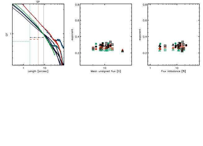
Figure 4.: SP cancellation functions. Left: Cancellation functions for selected magnetograms (in various colors). The cancellation functions with pixel size 0.32^′′are normalized to unity at 18^′′and pixel size 0.16^′′at 9^′′. Vertical and horizontal lines mark ranges used for fitting the exponents ($\kappa_{\mathrm{S}}$ in green dotted line, $\kappa_{\mathrm{I}}$ in red dashed line, and $\kappa_{\mathrm{L}}$ in black dash-dotted line). The same colors are used in all plots to differentiate between the spatial scales. Middle: Cancellation exponents as a function of $\langle|B_{z}|\rangle$. Error bars show 1$\sigma_{\mathrm{fit}}$. Circle symbols are rasters with exposure times less than 2 s, diamonds are exposure times between 2 and 5 s, and squares are exposure times longer than 5 s. Right: Exponents as a function of flux imbalance. fig:sp-all

The dependence of MDI and HMI cancellation exponents on $\langle|B_{z}|\rangle$ and flux imbalance suggest that the presence of magnetic network elements in the magnetograms influences the cancellation exponents. (Magnetic network flux is stronger than the intra-network, the network is mostly unipolar, and occurs at scales of a few tens of arcseconds.) To model the effect on $\chi(l)$ of a large (active-region-remnant or network-like) unipolar flux region, our observation region $\mathcal{A}$ is decomposed into two sub-regions: $\mathcal{B}$ (containing intra-network quiet-Sun in which a scaling $\chi(l)$ would be found) and the unipolar flux concentration $\mathcal{C}$ (over which $\int_{\mathcal{C}}|B_{z}|\mathrm{d}a=\big{|}\int_{\mathcal{C}}B_{z}\mathrm{d}a\big{|}$, i.e., there is no cancellation). Our goal is to find the cancellation function [$\chi^{\prime}(l)$] over the entire region $\mathcal{A}=\mathcal{B}\cup\mathcal{C}$. We consider only scales $l\ll$ the size of the unipolar flux concentration. So, a given square $\mathcal{A}_{i}(l)$ is either in $\mathcal{B}$ or $\mathcal{C}$,

$$\chi^{\prime}(l)=\frac{\sum_{\mathcal{A}_{i}(l)\in\mathcal{B}}\bigg{|}\int_{\mathcal{A}_{i}(l)}B_{z}\mathrm{d}a\bigg{|}+\sum_{\mathcal{A}_{i}(l)\in\mathcal{C}}\bigg{|}\int_{\mathcal{A}_{i}(l)}B_{z}\mathrm{d}a\bigg{|}}{\int_{\mathcal{B}}|B_{z}|\mathrm{d}a+\int_{\mathcal{C}}|B_{z}|\mathrm{d}a}\,.$$ (5)

Using $\sum_{\mathcal{A}_{i}(l)\in\mathcal{C}}\bigg{|}\int_{\mathcal{A}_{i}(l)}B_{z}\mathrm{d}a\bigg{|}=\int_{\mathcal{C}}|B_{z}|\mathrm{d}a$ and defining
$P=\int_{\mathcal{C}}|B_{z}|\mathrm{d}a/\int_{\mathcal{B}}|B_{z}|\mathrm{d}a$, the ratio of mean unsigned flux in the unipolar flux concentration compared to the rest of the region, we find

$$\chi^{\prime}(l)=\frac{\chi(l)+P}{1+P}\,.$$ (6)

Assuming that the intra-network quiet-Sun flux is completely balanced, flux imbalance (FI) is given by

$$\mathrm{FI}=\frac{\bigg{|}\int_{\mathcal{A}}B_{z}\mathrm{d}a\bigg{|}}{\int_{\mathcal{A}}\big{|}B_{z}\big{|}\mathrm{d}a}=\frac{P}{1+P}\,.\ilabel{eq:fip}$$ (7)

We take $\chi(l)$ from the HMI magnetogram with the smallest flux imbalance and employ Equations (eq:model) and (eq:fip) to plot synthetic $\chi^{\prime}(l)$ versus flux imbalance in Figure fig:unipolar. The synthetic exponents as a function of flux imbalance mimic the MDI and HMI observations: Small increases in the imbalance do not alter the exponent, while imbalances above $\approx$10% lead to a decreasing $\kappa$. The model explains the observed dependence of $\kappa$ on flux imbalance as a consequence of unipolar network magnetic fields altering the cancellation function. Note that the dependence of the exponents on $\langle|B_{z}|\rangle$ applies also to magnetograms with very small imbalances. Small imbalances imply that the positive and negative network concentrations balance out each other, not that there is only a small amount of network flux present.

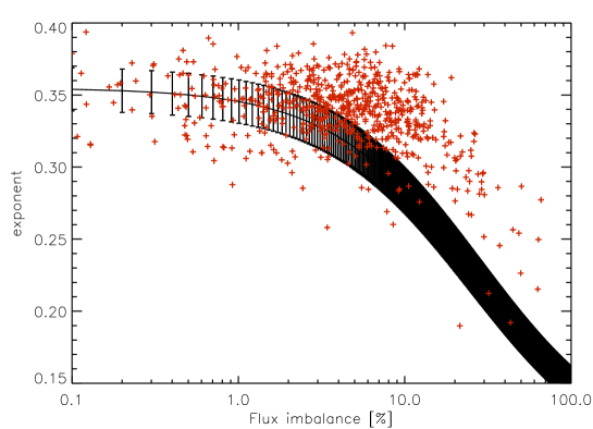
Figure 5.: Effect of flux imbalance. Synthetic cancellation exponents for intermediate scale $\kappa_{\mathrm{I}}$ as a function of flux imbalance. Error bars are 1$\sigma_{\mathrm{\mathrm{fit}}}$. Measured HMI $\kappa_{\mathrm{I}}$ are shown as red crosses.fig:unipolar

3.2 Intra-Network Exponents

Since the cancellation exponents are affected by the presence of network elements, a combination of smoothing and thresholding can be applied to mask out all the network pixels in the magnetograms prior to computing the cancellation functions. An example of a mask applied to an HMI magnetogram is shown in Figure fig:mask. To test how the masking affects the measured exponents, we apply a network mask to a synthetic magnetogram consisting of pure noise ($\kappa_{\mathrm{noise}}=1$) and compare the exponents from the masked and unmasked magnetograms: The effect on the exponent is smaller than the error in the fit.

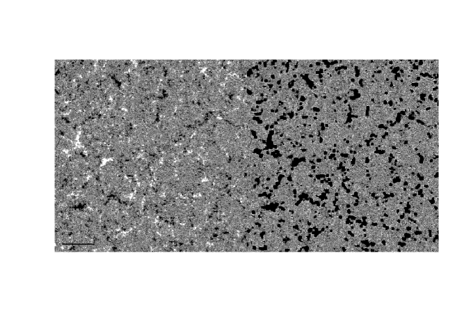
Figure 6.: Masking of network. Left: Original HMI magnetogram with network elements. Right: Same magnetogram with network elements masked out. The color scales saturate at $\pm$25 G. The horizontal line in the bottom left corner shows the spatial scale of 50^′′. fig:mask

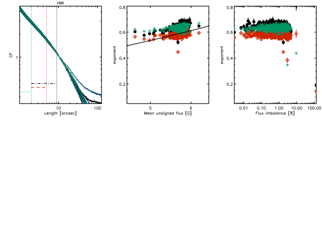
Figure 7.: HMI cancellation functions for intra-network (network masked out) magnetograms. Left: Cancellation functions for selected magnetograms (in various colors) normalized to unity at 9^′′. Vertical and horizontal lines mark ranges used for fitting the exponents ($\kappa_{\mathrm{S}}$ in green dotted line and crosses, $\kappa_{\mathrm{I}}$ in red dashed line and diamonds, and $\kappa_{\mathrm{L}}$ in black dash-dotted line and circles). The same colors and symbols are used in all plots to differentiate between the spatial scales. Middle: Cancellation exponents as a function of $\langle|B_{z}|\rangle$. Solid black line shows linear fit, slope 0.3, of $\kappa$ vs. $\log$$\langle|B_{z}|\rangle$. Error bars show 1$\sigma_{\mathrm{fit}}$. Right: Exponents as a function of flux imbalance. The systematic dependence is seen to be effectively removed.fig:hmi-qs

Masking out the network pixels in the HMI magnetograms to measure the “true” intra-network cancellation exponents (Figure fig:hmi-qs and Table table:inw) leads to significantly higher values for $\kappa_{\mathrm{L}}$ and $\kappa_{\mathrm{I}}$. $\kappa$ still depends on $\langle|B_{z}|\rangle$, but in the opposite sense than in the unmasked magnetograms: In the intra-network magnetograms $\kappa$ increases with increasing $\langle|B_{z}|\rangle$. This demonstrates that the decrease of $\kappa$ with increasing $\langle|B_{z}|\rangle$ in the unmasked magnetograms was due to the presence of the network elements. A linear fit of intra-network magnetogram $\kappa$ vs.  $\log$($\langle|B_{z}|\rangle$) gives a slope of $\approx$0.3. This increase of $\kappa$ with $\langle|B_{z}|\rangle$ can be understood from Equation (eq:model). An increase in flux imbalance means more pixels that are never canceled out at any scale, a flattening of the cancellation function, and a decrease in $\kappa$. A magnetogram with very weak signal can be out of balance from a small number of moderately strong pixels of the same sign. In fact, we see in Figure fig:for-j that nearly all magnetograms with over 1% flux imbalance, have $\langle|B_{z}|\rangle$$<\,5.5\,$G. The weakest magnetograms have greater flux imbalances and, consequently, smaller $\kappa$.

Figure 8.: Flux imbalance in masked HMI magnetograms vs. $\langle|B_{z}|\rangle$. fig:for-j

The network masking of MDI magnetograms was not entirely successful and effects of network are still visible in the $\langle|B_{z}|\rangle$ and flux imbalance plots. Compared to HMI, the effect of masking the magnetograms is small in MDI (Figure fig:mdi-inw and Table table:inw). The modest change may also be partially due to the network vs. intra-network contrast being smaller in MDI than HMI. The intra-network SP exponents (Figure fig:sp-qs and Table table:inw2) are increased on all scales. The change is largest for longer exposures and large spatial scales. Since the longer exposure times have less noise and their $\kappa$ values increase the most after removal of the network, the increase in $\kappa$ cannot be due to noise alone.

Figure 9.: MDI intra-network (network masked out) cancellation functions. Left: Cancellation functions for selected magnetograms (in various colors) normalized to unity at 9^′′. Vertical and horizontal lines mark ranges used for fitting the exponents ($\kappa_{\mathrm{S}}$ in green dotted line and crosses, $\kappa_{\mathrm{I}}$ in red dashed line and diamonds, and $\kappa_{\mathrm{L}}$ in black dash-dotted line and circles). The same colors and symbols are used in all plots to differentiate between the scales. Middle: Cancellation exponents as a function of $\langle|B_{z}|\rangle$. Error bars show 1$\sigma_{\mathrm{fit}}$. Right: Exponents as a function of flux imbalance. fig:mdi-inw

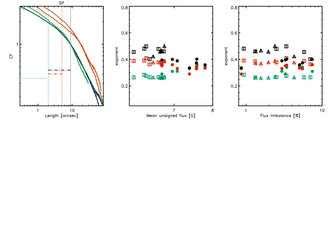
Figure 10.: SP intra-network (network masked out) cancellation functions. Left: Cancellation functions for selected magnetograms (in various colors). The cancellation functions with pixel size 0.32^′′are normalized to unity at 18^′′and pixel size 0.16^′′at 9^′′. Vertical and horizontal lines mark ranges used for fitting the exponents ($\kappa_{\mathrm{S}}$ in green dotted line, $\kappa_{\mathrm{I}}$ in red dashed line, and $\kappa_{\mathrm{L}}$ in black dash-dotted line). The same colors are used in all plots to differentiate between the spatial scales. Middle: Cancellation exponents as a function of $\langle|B_{z}|\rangle$. Error bars show 1$\sigma_{\mathrm{fit}}$. Circle symbols are rasters with exposure times less than 2 s, diamonds are exposure times between 2 and 5 s, and squares are exposure times longer than 5 s. Most of the scatter is due to differing exposure times. Right: Exponents as a function of flux imbalance. fig:sp-qs

Table 2.: Power-law fits for intra-network (network masked out) cancellation functions for HMI, MDI, and SP magnetograms.table:inw

table:inw2 Mean Standard deviation HMI $\kappa_{\mathrm{S}}$ 0.63 0.024 $\kappa_{\mathrm{I}}$ 0.58 0.024 $\kappa_{\mathrm{L}}$ 0.64 0.084 MDI $\kappa_{\mathrm{S}}$ 0.59 0.055 $\kappa_{\mathrm{I}}$ 0.46 0.077 $\kappa_{\mathrm{L}}$ 0.46 0.089 SP $t_{\mathrm{exp}}<$2s $\kappa_{\mathrm{S}}$ 0.32 0.020 $\kappa_{\mathrm{I}}$ 0.32 0.017 $\kappa_{\mathrm{L}}$ 0.38 0.017 $t_{\mathrm{exp}}>$2s $\kappa_{\mathrm{S}}$ 0.28 0.0063 $\kappa_{\mathrm{I}}$ 0.38 0.014 $\kappa_{\mathrm{L}}$ 0.48 0.036
¹Only magnetograms with no network remnants are included.

3.3 Effect of Noise and Seeing

sec:noise

An examination of Tables table:sp and table:inw suggests that the cancellation exponent is larger for noisier instruments and shorter exposures, i.e., for noisier magnetograms. We now demonstrate that this is the case by artificially adding noise to our magnetograms. The first panel in Figure fig:noise shows how an HMI cancellation function changes as random-distributed noise is incrementally added to the magnetogram prior to computing $\chi(l)$. Adding noise changes first the smallest scales. As the amount of noise increases the scales affected by noise also increase. For HMI adding 1 G (random numbers with a mean of zero and a standard deviation of one) of noise does not change the cancellation function noticeably and only a small difference is seen for 3 G. In contrast, adding noise at the 6 and 15 G levels, respectively, significantly alters $\chi(l)$ on increasing spatial scales. That no change is visible for $3\,$G, gives us a measure of noise in the HMI magnetogram: between 3 and $6\,$G.

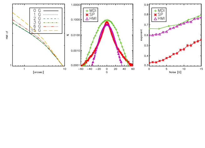
Figure 11.: Noise and $\chi(l)$. Left: HMI intra-network cancellation functions with increasing artificial noise (see figure legend). Middle: Histograms of intra-network magnetic flux. Right: Small-scale exponents as a function of added noise. For the SP magnetogram we use a raster taken with a 1.6 s exposure time.fig:noise

The remaining panels in Figure fig:noise show how the small scale cancellation exponents for the different instruments react to increased noise. (Noise was added in units of counts (1 count = 2.81 G) to the MDI magnetograms.) All of the $\kappa_{\mathrm{S}}$, as a function of noise curves, have the same general shape (rightmost panel in Figure fig:noise): They start with a plateau and after an instrument-specific threshold (magnetogram noise level) is reached, $\kappa_{\mathrm{S}}$ begins to increase linearly as a function of added noise. The nominal noise values (upper limits) of the different instruments can be defined as the full width at half maximum of Gaussian fits to the magnetic flux histograms. The widths are 31.6 G for MDI, 21.1 G for HMI, and 13.5 G for SP. In the linear increase regime the increase in $\kappa$ per added noise is 0.01 per G for MDI and 0.02 per G for SP and HMI. The length of the plateau and steepness of the increase are related to the inherent noise in the data: The less instrumental noise there is, the more sensitive the cancellation function is to added noise. SP, which has the lowest nominal noise level, has the shortest plateau and steepest increase, while MDI, the noisiest instrument, is less sensitive to noise. Consistent with the noise experiment, SP has the smallest measured exponents and MDI the largest, suggesting that MDI magnetograms are more strongly affected by noise.

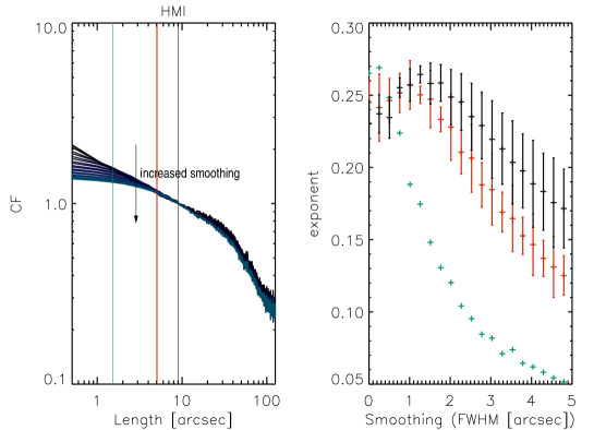
Figure 12.: Effects of spatial smoothing. Left: HMI cancellation functions computed with increased spatial smoothing (Gaussian smoothing with full width at half maximum (FWHM) increasing in increments of 0.5 pixels). Right: Exponents as a function of Gaussian FWHM ($\kappa_{\mathrm{S}}$ in green, $\kappa_{\mathrm{I}}$ in red and $\kappa_{\mathrm{L}}$ in black).fig:hmi-smooth

Figure fig:hmi-smooth shows how spatial smoothing changes the cancellation function. The effect of smoothing is opposite to that of increasing the noise (recall that $\kappa=0$ for a smooth field and $k=1$ for noise). The exponents decrease with increased spatial smoothing. This demonstrates how seeing conditions and spatial over-sampling can reduce the measured exponents.

4 Conclusions

Significant artifacts in measuring the cancellation function from current observations have been identified. The cancellation exponent is sensitive to noise level differences between instruments: Noise increases both $\kappa$ and the scatter between individual measurements of $\kappa$. Not surprisingly, $\kappa$ decreases by seeing and spatial over-sampling. We also find that $\kappa$ is sensitive within a single instrument’s observations to magnetic flux imbalances and mean unsigned flux. A simple model suggests that this dependence is the effect of network elements: They reduce $\kappa$. This simple model also explains why the value of $\kappa$ calculated in PGDS2009 and St2011 differ: The network is enhanced in the latter study, decreasing $\kappa$.

Of all the observational artifacts, the effect of the network can be removed by masking network elements out of magnetograms. We then find values of $\kappa_{I}\approx 0.58$ for HMI and $\kappa_{I}\approx 0.38$ for SP. (For MDI the removal of network was not fully successful and the dependence of $\chi(l)$ on the presence of network elements was not entirely removed.) The difference in $\kappa$ between HMI and SP is due to HMI magnetograms being demonstrably more noisy: HMI’s noise level is $\approx 4\,$G and SP’s is $\approx 2\,$G, at least for determinations of the cancellation exponent (see Figure fig:noise). Since noise first affects the smallest scales of the cancellation function, high resolution (diffraction limit, pixel size, and seeing) observations with minimal noise are needed to measure the exponent on scales below a couple of arcseconds. Therefore, no conclusive value of the unsigned flux can be given by cancellation function analysis with current instruments.

An upper bound of the unsigned flux is the best that can be done with the available data. Since SP has the lowest noise level, we can safely conclude $\kappa\lessapprox 0.38$. The quiet-Sun magnetic field is not a completely self-similar field: It will become smooth over an order-of-magnitude in scales near the magnetic diffusion scale (below which there is no further cancellation). However, using $\kappa\lessapprox 0.38$ and that the power-law ends at $l_{0}\geq 80\,$m (the magnetic diffusion scale estimate from PGDS2009) in Equation (eq:extrapolate), we have an upper bound on the true mean unsigned flux. We find that $\langle|B_{z}|\rangle_{\mathrm{true}}\equiv\mathrm{Flux}_{0}\lessapprox 268\,$G (standard deviation 44 G) from SP data with exposure times longer than 5 s. (Note that if the power-law for some reason ends at even larger scales than the $\approx 800\,$m beginning of the diffusive range, this bound still holds.) The noisier instruments, MDI and HMI, give significantly higher values. Both the noise level and sensitivity of the instruments affect the estimates. SP being the least noisy of the instruments can be considered as an upper bound for the flux. MaSaLaDeTrBu2006 found a similar upper bound, $\langle|B_{z}|\rangle_{\mathrm{true}}\lessapprox 200-300\,$G from the scattering line polarization of Ce ii.

We found no correlation between $\kappa$ and global mean unsigned flux: The small scale ($<$10^′′) field distribution/fractal geometry is not affected by the global magnetic configuration, at least not during a rising phase of the cycle sampled by HMI. A study of HMI cancellation functions from the end of the previous solar minimum past the next solar maximum may show how flux from decaying active regions affects the flux distribution in the quiet Sun, and possibly give indications of the relative importance of possible quiet-Sun small-scale dynamo action in different phases of the solar activity cycle.

It should be emphasized that the present analysis and findings are for quiet Sun magnetic fields which are known to be turbulent. Issues identified in the analysis most likely do not affect as strongly measurements of active region fractal dimensions. The significance of noise in the cancellation statistics may extend to the studies of fractal dimensions and flaring probability (e.g., Georgoulis2011). Based on the current analysis, using less-noisy magnetograms, such as HMI, may show the fractal dimension of the magnetic flux to still have some predictive capability for flaring active regions. To establish the usability of fractal analysis for flare forecasting, however, a large sample of flaring and non-flaring active region magnetograms with little noise is needed. A statistical study of flaring and non-flaring HMI vector magnetograms could also be used to address the differences of using line of sight flux and current helicity for predictions.

Acknowledgement

JPG gratefully acknowledges the support of the U.S. Department of Energy through the LANL/LDRD Program for this work. Hinode is a Japanese mission developed and launched by ISAS/JAXA, with NAOJ as domestic partner and NASA and STFC (UK) as international partners. It is operated by these agencies in co-operation with ESA and NSC (Norway) Data provided by the SOHO/MDI consortium. SOHO is a mission of international cooperation between ESA and NASA. SDO is a mission for NASA’s Living With a Star program.

Appendix

For a completely self-similar field, knowledge of net flux at any scale and of the power-law scaling exponent implies knowledge of net flux at all scales and, hence, the unsigned flux. This is most easily seen in the example of a vertical random field [$f_{z}$]. For a random field, the integral over an area is proportional to the square root of the area (random walk),

$$\bigg{|}\int_{\mathcal{A}_{i}(l)\in\mathcal{A}}f_{z}\mathrm{d}a\bigg{|}\propto l\,,$$ (8)

while the integral over a strictly positive field is proportional to its area,

$$\int_{\mathcal{A}_{i}(l)\in\mathcal{A}}|f_{z}|\mathrm{d}a\propto l^{2}\,.$$ (9)

Therefore,

$$\chi(l)\propto\frac{1}{l}\,,$$ (10)

and we identify $\kappa=1$ for pure noise. For scales smaller than the correlation length of the noise, the net flux is equal to the unsigned flux,

$$\mathrm{Flux}_{l}=\mathrm{Flux}_{0}\qquad\forall l\leq l_{0}\,,\ilabel{eq:kappais1a}$$ (11)

and for larger scales,

$$\mathrm{Flux}_{l}=\frac{C}{l}\qquad\forall l\geq l_{0}\,.\ilabel{eq:kappais1b}$$ (12)

The constant $C$ is determined by equating Equations (eq:kappais1a) and (eq:kappais1b) at the correlation length, $l=l_{0}$:

$$\frac{\mathrm{Flux}_{l}}{\mathrm{Flux}_{0}}=\frac{l_{0}}{l}\qquad\forall l\geq l_{0}\,.\ilabel{eq:kappais1c}$$ (13)

This power-law dependence, Equation. (eq:kappais1c), is shown in Figure fig:kappais1. This means that the unsigned flux can be exactly calculated given the net flux at any scale and the scale at the end of the power-law, $l_{0}$,

$$\mathrm{Flux}_{0}=\mathrm{Flux}_{l}\frac{l}{l_{0}}\,,$$ (14)

for a random field. For any other purely self-similar field with cancellation exponent $\kappa$,

$$\mathrm{Flux}_{l}=\mathrm{Flux}_{L}\big{(}\frac{L}{l}\big{)}^{\kappa}\qquad\forall l,L\geq l_{0}\,.\ilabel{eq:extrapolate}$$ (15)

For the extreme case of a unipolar field, $\kappa=0$ and $\mathrm{Flux}_{l}=\mathrm{Flux}_{0}$ for all scales $l$. In general, $0\leq\kappa\leq 1$.

Figure 13.: Ratio of net flux to unsigned flux $\chi(l)$ versus scale ($l$) for noise with correlation length $l_{0}$. The ratio is given by $\frac{l_{0}}{l}$ (dashed line).fig:kappais1

References

- Abramenko (2003) Abramenko, V.: 2003, Pre-flare changes in current helicity and turbulent regime of the photospheric magnetic field. Adv. Space Res. 32, 1937.
- Abramenko and Yurchyshyn (2010a) Abramenko, V., Yurchyshyn, V.: 2010a, Intermittency and multifractality spectra of the magnetic field in solar active regions. ApJ 722, 122.
- Abramenko and Yurchyshyn (2010b) Abramenko, V., Yurchyshyn, V.: 2010b, Magnetic energy spectra in solar active regions. ApJ 720, 717.
- Brandenburg (1995) Brandenburg, A.: 1995, Flux tubes and scaling in MHD dynamo simulations. Chaos Solitons Fractals 5, 2023.
- Brandenburg et al. (1992) Brandenburg, A., Procaccia, I., Segel, D., Vincent, A.: 1992, Fractal level sets and multifractal fields in direct simulations of turbulence. Phys. Rev. A 46, 4819.
- Cadavid et al. (1994) Cadavid, A.C., Lawrence, J.K., Ruzmaikin, A.A., Kayleng-Knight, A.: 1994, Multifractal models of small-scale solar magnetic fields. ApJ 429, 391.
- Frisch (1995) Frisch, U.: 1995, Turbulence. The legacy of A. N. Kolmogorov. Cambridge University Press. 136-148, 185-189 Cambridge.
- Georgoulis (2012) Georgoulis, M.K.: 2012, Are solar active regions with major flares more fractal, multifractal, or turbulent than others? Sol. Phys. 276, 161.
- Goldreich and Sridhar (1995) Goldreich, P., Sridhar, S.: 1995, Toward a theory of interstellar turbulence. 2: Strong Alfvénic turbulence. ApJ 438, 763.
- Goode et al. (2010) Goode, P.R., Yurchyshyn, V., Cao, W., Abramenko, V., Andic, A., Ahn, K., Chae, J.: 2010, Highest resolution observations of the quietest Sun. ApJ 714, L31.
- Iroshnikov (1964) Iroshnikov, P.S.: 1964, Turbulence of a conducting fluid in a strong magnetic field. Soviet Ast. 7, 566.
- Janßen, Vögler, and Kneer (2003) Janßen, K., Vögler, A., Kneer, F.: 2003, On the fractal dimension of small-scale magnetic structures in the Sun. A&A 409, 1127.
- Kraichnan (1965) Kraichnan, R.H.: 1965, Inertial-range spectrum of hydromagnetic turbulence. Phys. Fluids 8, 1385.
- Lee et al. (2010) Lee, E., Brachet, M.E., Pouquet, A., Mininni, P.D., Rosenberg, D.: 2010, Lack of universality in decaying magnetohydrodynamic turbulence. Phys. Rev. E 81, 016318.
- Lites et al. (2008) Lites, B.W., Kubo, M., Socas-Navarro, H., Berger, T., Frank, Z., Shine, R., et al.2008, The horizontal magnetic flux of the quiet-Sun internetwork as observed with the Hinode Spectro-Polarimeter. ApJ 672, 1237.
- Manso Sainz, Landi Degl’Innocenti, and Trujillo Bueno (2006) Manso Sainz, R., Landi Degl’Innocenti, E., Trujillo Bueno, J.: 2006, A qualitative interpretation of the second solar spectrum of Ce ll. A&A 447, 1125.
- Moll et al. (2011) Moll, R., Pietarila Graham, J., Pratt, J., Cameron, R.H., Müller, W.-C., Schüssler, M.: 2011, Universality of the small-scale dynamo mechanism. ApJ 736, 36.
- Ott et al. (1992) Ott, E., Du, Y., Sreenivasan, K.R., Juneja, A., Suri, A.K.: 1992, Sign-singular measures - Fast magnetic dynamos, and high-Reynolds-number fluid turbulence. Phys. Rev. Lett. 69, 2654.
- Pietarila Graham, Cameron, and Schüssler (2010) Pietarila Graham, J., Cameron, R., Schüssler, M.: 2010, Turbulent small-scale dynamo action in solar surface simulations. ApJ 714, 1606. http://stacks.iop.org/0004-637X/714/i=2/a=1606?key=crossref.c8866af85337f716c98e702d39990156.
- Pietarila Graham, Danilovic, and Schüssler (2009) Pietarila Graham, J., Danilovic, S., Schüssler, M.: 2009, Turbulent magnetic fields in the quiet Sun: Implications of Hinode observations and small-scale dynamo simulations. ApJ 693, 1728.
- Pietarila Graham, Mininni, and Pouquet (2005) Pietarila Graham, J., Mininni, P.D., Pouquet, A.: 2005, Cancellation exponent and multifractal structure in two-dimensional magnetohydrodynamics: Direct numerical simulations and Lagrangian averaged modeling. Phys. Rev. E 72, 045301.
- Pietarila Graham, Mininni, and Pouquet (2011) Pietarila Graham, J., Mininni, P.D., Pouquet, A.: 2011, High Reynolds number magnetohydrodynamic turbulence using a Lagrangian model. Phys. Rev. E 84, 016314.
- Sánchez Almeida and Martínez González (2011) Sánchez Almeida, J., Martínez González, M.: 2011, The magnetic fields of the quiet Sun. In: Kuhn, J.R. Harrington, D.M. Lin, H. Berdyugina, S.V. Trujillo-Bueno, J. Keil, S.L. Rimmele, T. (eds.), Solar Polarization 6, ASP Conf. Ser., 437 451.
- Scherrer et al. (1995) Scherrer, P.H., Bogart, R.S., Bush, R.I., Hoeksema, J.T., Kosovichev, A.G., Schou, J., et al.1995, The Solar Oscillations Investigation - Michelson Doppler Imager. Sol. Phys. 162, 129.
- Scherrer et al. (2012) Scherrer, P.H., Schou, J., Bush, R.I., Kosovichev, A.G., Bogart, R.S., Hoeksema, J.T., et al.2012, The Helioseismic and Magnetic Imager (HMI) Investigation for the Solar Dynamics Observatory (SDO). Sol. Phys. 275, 207.
- Solanki et al. (2010) Solanki, S.K., Barthol, P., Danilovic, S., Feller, A., Gandorfer, A., Hirzberger, J., et al.2010, SUNRISE: Instrument, mission, data, and first results. ApJ 723, L127.
- Sorriso-Valvo et al. (2002) Sorriso-Valvo, L., Carbone, V., Noullez, A., Politano, H., Pouquet, A., Veltri, P.: 2002, Analysis of cancellation in two-dimensional magnetohydrodynamic turbulence. Phys. Plasmas 9, 89.
- Sorriso-Valvo et al. (2003) Sorriso-Valvo, L., Abramenko, V., Carbone, V., Noullez, A., Politano, H., Pouquet, A., Veltri, P., Yurchyshyn, V.: 2003, Cancellations analysis of photospheric magnetic structures and flares. Mem. Soc. Astron. Italiana 74, 631.
- Sorriso-Valvo et al. (2004) Sorriso-Valvo, L., Carbone, V., Veltri, P., Abramenko, V.I., Noullez, A., Politano, H., Pouquet, A., Yurchyshyn, V.: 2004, Topological changes of the photospheric magnetic field inside active regions: A prelude to flares? Planet. Space Sci. 52, 937.
- Stenflo (2011) Stenflo, J.O.: 2011, Collapsed, uncollapsed, and hidden magnetic flux on the quiet Sun. A&A 529, A42.
- Tsuneta et al. (2008) Tsuneta, S., Ichimoto, K., Katsukawa, Y., Nagata, S., Otsubo, M., Shimizu, T., et al.2008, The Solar Optical Telescope for the Hinode mission: An overview. Sol. Phys. 249, 167.