Overdamped dynamics of long-range systems on a one-dimensional lattice: Dominance of the mean-field mode and phase transition

Abstract

We consider the overdamped dynamics of a paradigmatic long-range system of particles residing on the sites of a one-dimensional lattice, in the presence of thermal noise. The internal degree of freedom of each particle is a periodic variable which is coupled to those of other particles with an attractive $XY$-like interaction. The coupling strength decays with the interparticle separation $r$ in space as $1/r^{\alpha}$;  $0<\alpha<1$. We study the dynamics of the model in the continuum limit by considering the Fokker-Planck equation for the evolution of the spatial density of particles. We show that the equation allows a linearly stable stationary state which is always uniform in space, being non-uniform in the internal degrees below a critical temperature $T=1/2$ and uniform above, with a phase transition between the two at $T=1/2$. The state is the same as the equilibrium state of the mean-field version of the model, obtained by considering $\alpha=0$. Our analysis also lets us to compute the growth and decay rates of spatial Fourier modes of density fluctuations. The growth rates compare very well with numerical simulations.

I Introduction

In long-range interacting systems, the interparticle potential in $d$ dimensions decays at large separation, $r$, as $1/r^{\alpha}$, with $0\leq\alpha\leq d$ review1 ; review2 ; review3 . Examples are gravitational systems Chavanis:2006 , plasmas Escande:2010 , two-dimensional hydrodynamics Bouchet:2012 , charged and dipolar systems Bramwell:2010 , etc. Long-range systems are non-additive, and have equilibrium properties unusual for short-range systems, e.g., inequivalence of statistical ensembles Barre:2001 . Besides, they show intriguing dynamical features, e.g., broken ergodicity Mukamel:2005 and slow relaxation towards equilibrium Mukamel:2005 ; Yamaguchi:2004 .

A paradigmatic example of long-range systems is the so-called Hamiltonian mean-field (HMF) model, comprising a system of $N$ interacting particles evolving under Hamilton dynamics Ruffo:1995 . The $i$th particle, $i=1,2,\ldots,N$, has an internal degree of freedom $\theta_{i}$, a periodic variable of period $2\pi$. The $\theta_{i}$’s are coupled to one another via an attractive $XY$-like interaction $\sim-\cos(\theta_{i}-\theta_{j})$ between the $i$th and $j$th particles, with the coupling strength being of the “mean-field” type: It is equal for every pair of particles. As a result, the model is defined without requiring any lattice structure for the particles to reside on. In this model, a wide class of initial distributions relaxes to the Boltzmann-Gibbs equilibrium state over times that diverge with the system size Yamaguchi:2004 . As a consequence, the system in the thermodynamic limit does not ever attain equilibrium, instead it remains trapped in intermediate quasistationary states. Besides the HMF model, these states have been observed in a wide variety of long-range systems ranging from models with spin dynamics Gupta:2011 and plasma physics Levin:2008 to one-dimensional and two-dimensional gravity Joyce:2011 ; Levin:2010 . The HMF model is a prototype for systems with unscreened long-range interactions leading to long-lived spatially inhomogeneous states. Moreover, the model does not have a singularity at short length scales so that one can exclusively focus on effects of long-range interactions, in a way similar to studies of gravitational systems where a short-range softening is introduced Binney .

To explore how far the results obtained within the HMF model extend beyond its setting of mean-field coupling, the model has been considered on a one-dimensional periodic lattice on the sites of which the particles reside. Particles on different sites are coupled as in the HMF model, with the difference that the coupling strength decays with their separation $r$ along the lattice length as $1/r^{\alpha}$, with $0<\alpha<1$. The resulting model is known as the $\alpha$-HMF model Anteneodo:1998 . The HMF model is recovered on considering $\alpha=0$. Within a canonical ensemble, the $\alpha$-HMF model has the same equilibrium state as those of the HMF model Campa:2000-2003 . There have been many studies dealing with various dynamical aspects of the $\alpha$-HMF model that have illustrated their difference from those of the HMF model, e.g., Lyapunov exponents ineq1 ; ineq2 , and others ineq3 ; ineq4 . Hence, the equivalence of the equilibrium state of the two models raises an immediate question: How does the dynamics of the $\alpha$-HMF model lead to the same equilibrium state as that of its mean-field counterpart, the HMF model? This work is a step towards answering this question regarding the mean-field dominance in dictating the equilibrium state.

To address the issue, let us consider the simple setting of the $\alpha$-HMF model evolving in the presence of thermal noise and dissipation. The $i$th particle has the equations of motion

$$\frac{d\theta_{i}}{dt}=p_{i},$$ (1)

$$\frac{dp_{i}}{dt}=-\gamma p_{i}+\frac{1}{\widetilde{N}}\sum_{j=1,j\neq i}^{N}\frac{\sin(\theta_{j}-\theta_{i})}{(|j-i|_{c})^{\alpha}}+\sqrt{\gamma}\eta_{i}(t),$$ (2)

where $p_{i}$ denotes the momentum of the $i$th particle, while $\gamma$ is the damping constant. The second term on the right hand side of Eq. (2) is the force on the $i$th particle arising from the interaction potential: The quantity $|j-i|_{c}$ is the closest distance on the periodic lattice between the $i$th and $j$th sites:

$$|j-i|_{c}={\rm min}(|j-i|,N-|j-i|),$$ (3)

while

$$\widetilde{N}=\sum_{j=1}^{N}(|j-i|_{c})^{-\alpha}~{}\forall~{}i.$$ (4)

From Eq. (2), since $\alpha<1$, the cumulative interaction of one particle with all the remaining particles with aligned $\theta$’s would diverge in the limit $N\to\infty$ in the absence of the normalization $\widetilde{N}$, which explains its inclusion Campa:2000-2003 . In Eq. (2), $\eta_{i}(t)$ is a Gaussian white noise:

$$\langle\eta_{i}(t)\rangle=0,$$ (5)

$$\langle\eta_{i}(t)\eta_{j}(t^{\prime})\rangle=2T\delta_{ij}\delta(t-t^{\prime}),$$ (6)

where $T$ denotes the temperature, while the angular brackets denote averaging over noise realizations. In this work, we take the Boltzmann constant to be unity. The equations of motion (1) and (2) describe the evolution of the $\alpha$-HMF model within a canonical ensemble. We note that for $\alpha=0$, these equations reduce to those of the Brownian mean-field model considered in Refs. Acebron:1998-2000 and Chavanis:2005 .

Here, we will study the overdamped limit of the equations of motion, (1) and (2); after a time rescaling, these equations then reduce to the following Langevin equation for the $i$th particle:

$$\frac{d\theta_{i}}{dt}=\frac{1}{\widetilde{N}}\sum_{j=1,j\neq i}^{N}\frac{\sin(\theta_{j}-\theta_{i})}{(|j-i|_{c})^{\alpha}}+\eta_{i}(t).$$ (7)

We analyze the dynamics (7) in the continuum limit $N\to\infty$, when the lattice becomes a continuous segment characterized by the spatial coordinate $s\in[0,1]$. In this limit, the local density of oscillators $\rho(\theta;s,t)$ evolves in time following a Fokker-Planck equation.

We show that the Fokker-Planck equation allows a stationary state which is uniform in both $\theta$ and $s$. By performing a linear stability analysis of such a state, we find that when it is unstable, different spatial Fourier modes of fluctuations have different critical temperatures below which the modes grow exponentially in time with different rates. The largest critical temperature, $T_{c,0}=1/2$, corresponds to the spatially independent zero Fourier mode, i.e. the mean-field mode. Above this temperature, all the Fourier modes decay in time, thereby stabilizing the uniform state. Below $T_{c,0}$, our numerical simulations starting from the uniform state show that the unstable non-zero Fourier modes, growing exponentially in time at short times, nevertheless decay at long times to zero. By contrast, the mean-field mode grows and reaches a non-zero value, corresponding to a non-uniform stationary state, i.e. a state which is uniform in $s$, but non-uniform in $\theta$. We perform a linear stability analysis of the non-uniform state to demonstrate that indeed at temperatures below $T_{c,0}$, all the Fourier modes of fluctuations decay in time, thereby stabilizing the non-uniform state.

The long time dominance of the mean-field mode leading to a stationary state always uniform in space, here observed in the alpha-HMF model evolving under the canonical and overdamped dynamics, has also been observed when the model evolves within a microcanonical ensemble. In the latter case, the dynamical equations are obtained from Eqs. (1) and (2) by substituting $\gamma=0$ Bachelard:2011 . In the case of microcanonical dynamics, this dominance was just a numerical observation with no theoretical justification, while within the canonical and overdamped dynamics, we show how the mean-field mode arises as a linearly stable stationary solution of the Fokker-Planck equation.

The paper is structured as follows. In section II, we introduce the continuum limit of the dynamics (7), and perform the linear stability analysis of the uniform stationary state. In section III, we present numerical simulations in support of the analysis, in particular, to show the agreement of the growth rates of the unstable modes, the decay at long times of the unstable non-zero modes at all temperatures $T<1/2$, and the associated dominance of the mean-field mode. In section IV, we perform the linear stability analysis of the non-uniform stationary state. We end the paper with conclusions and perspectives.

II Continuum limit: Uniform stationary state and dynamics of Fourier modes

In the continuum limit $N\to\infty$, the lattice of the system (7) is densely filled with sites. Let us introduce the variable $s=i/N$ to denote the spatial coordinate along the lattice length, such that in the continuum limit it becomes the continuous variable $s\in[0,1]$. In this limit, we define a local density of particles $\rho(\theta;s,t)$ such that of all particles located between $s$ and $s+ds$ at time $t$, the fraction $\rho(\theta;s,t)d\theta$ have their degrees of freedom between $\theta$ and $\theta+d\theta$. This density is non-negative, $2\pi$-periodic in $\theta$, and obeys the normalization

$$\int_{0}^{2\pi}d\theta~{}\rho(\theta;s,t)=1~{}~{}\forall~{}s.$$ (8)

In the continuum limit, the equation of motion is given by

$$\frac{\partial\theta(s,t)}{\partial t}=\kappa(\alpha)\int d\theta^{\prime}ds^{\prime}\frac{\sin(\theta^{\prime}-\theta)}{(|s^{\prime}-s|_{c})^{\alpha}}\rho(\theta^{\prime};s^{\prime},t)+\eta(s,t),$$

(9)

where

$$\kappa(\alpha)^{-1}=\int_{s-1/2}^{s+1/2}\frac{ds^{\prime}}{(|s^{\prime}-s|_{c})^{\alpha}},$$ (10)

and

$$|s^{\prime}-s|_{c}={\rm min}(|s^{\prime}-s|,1-|s^{\prime}-s|).$$ (11)

Also, we have

$$\langle\eta(s,t)\rangle=0,$$ (12)

$$\langle\eta(s,t)\eta(s^{\prime},t^{\prime})\rangle=2T\delta(s-s^{\prime})\delta(t-t^{\prime}).$$ (13)

The time evolution of $\rho(\theta;s,t)$ follows the Fokker-Planck equation

$$\frac{\partial\rho}{\partial t} = -\kappa(\alpha)\frac{\partial}{\partial\theta}\Big{[}\Big{(}\int d\theta^{\prime}ds^{\prime}\frac{\sin(\theta^{\prime}-\theta)}{(|s^{\prime}-s|_{c})^{\alpha}}\rho(\theta^{\prime};s^{\prime},t)\Big{)}\rho\Big{]}$$ (14)

$$+T\frac{\partial^{2}\rho}{\partial\theta^{2}}.$$

Its stationary solution, obtained by setting the left hand side to zero, is

$$\rho_{0}(\theta;s)\propto\exp\Big{[}\frac{\kappa(\alpha)}{T}\int d\theta^{\prime}ds^{\prime}\frac{\cos(\theta^{\prime}-\theta)}{(|s^{\prime}-s|_{c})^{\alpha}}\rho_{0}(\theta^{\prime};s^{\prime})\Big{]}.$$ (15)

Consider the particular stationary state which is uniform both in $\theta$ and in the spatial coordinate $s$,

$$\rho_{0}=\frac{1}{2\pi}.$$ (16)

This state, although stationary, might be destabilized by the thermal fluctuations inherent in the dynamics. Let us then analyze the stability, in particular, linear stability of the state with respect to small thermal fluctuations $\delta\rho(\theta;s,t)$. To this end, we write

$$\rho(\theta;s,t)=\frac{1}{2\pi}+\delta\rho(\theta;s,t);~{}~{}\delta\rho(\theta;s,t)\ll 1.$$ (17)

Substituting Eq. (17) into Eq. (14) and keeping terms to linear order in $\delta\rho$, we find that $\delta\rho$ satisfies

$$\frac{\partial\delta\rho}{\partial t} = \frac{\kappa(\alpha)}{2\pi}\int d\theta^{\prime}ds^{\prime}~{}\frac{\cos(\theta^{\prime}-\theta)}{(|s^{\prime}-s|_{c})^{\alpha}}\delta\rho(\theta^{\prime};s^{\prime},t)+T\frac{\partial^{2}\delta\rho}{\partial\theta^{2}}.$$

Expressing $\delta\rho$ in terms of its Fourier series with respect to the periodic variable $\theta$ as

$$\delta\rho(\theta;s,t)=\sum_{k=-\infty}^{\infty}\widehat{\delta\rho}_{k}(s,t)e^{ik\theta},$$ (19)

we find from Eq. (LABEL:linearized-equation) that only the modes $k=\pm 1$ are affected by the coupling between the particles, and that $\widehat{\delta\rho}_{\pm 1}$ satisfies

$$\frac{\partial\widehat{\delta\rho}_{\pm 1}}{\partial t}=\frac{\kappa(\alpha)}{2}\int ds^{\prime}\frac{\widehat{\delta\rho}_{\pm 1}(s^{\prime},t)}{(|s^{\prime}-s|_{c})^{\alpha}}-T\widehat{\delta\rho}_{\pm 1}.$$ (20)

One thus gets a set of equations for each position $s$, all coupled together by the second term on the right hand side of Eq. (20). For $k\neq\pm 1$, one has

$$\frac{\partial\widehat{\delta\rho}_{\pm k}}{\partial t}=-T\widehat{\delta\rho}_{\pm k};~{}~{}k\neq 1.$$ (21)

Thus, $\widehat{\delta\rho}_{\pm k}(s,t)$ for $k\neq 1$ decays exponentially in time as $\exp(-Tt)$, so that these modes cannot destabilize the uniform state (16).

Since we have a periodic lattice, to solve Eq. (20), we next consider the spatial Fourier series of $\widehat{\delta\rho}_{\pm 1}(s,t)$:

$$\widehat{\delta\rho}_{\pm 1}(s,t)=\sum_{m=-\infty}^{\infty}\overline{\delta\rho}_{\pm 1,m}(t)e^{i2\pi ms}.$$ (22)

On substituting in Eq. (20), we get

$$\frac{\partial\overline{\delta\rho}_{\pm 1,m}}{\partial t}=\frac{\kappa(\alpha)\Lambda_{m}(\alpha)}{2}\overline{\delta\rho}_{\pm 1,m}-T\overline{\delta\rho}_{\pm 1,m},$$ (23)

where

$$\Lambda_{m}(\alpha) = \int_{s-1/2}^{s+1/2}ds^{\prime}~{}\frac{e^{i2\pi m(s^{\prime}-s)}}{(|s^{\prime}-s|_{c})^{\alpha}}.$$ (24)

Note that $\Lambda_{m}(\alpha)=\Lambda_{-m}(\alpha)$. It is known that $\Lambda_{m}(\alpha)\geq 0$, and that it is a monotonically decreasing function of $|m|$ when $m$ is an integer; moreover, $\Lambda_{m}(\alpha)\to 0$ as $m\to\pm\infty$ Gupta:2012 .

Equation (23) has the solution

$$\overline{\delta\rho}_{\pm 1,m}(t)=\exp\Big{[}\Big{(}\frac{\kappa(\alpha)\Lambda_{m}(\alpha)}{2}-T\Big{)}t\Big{]}\overline{\delta\rho}_{\pm 1,m}(0).$$ (25)

It then follows from our linear stability analysis that the $m$th spatial mode of fluctuations $\overline{\delta\rho}_{\pm 1,m}(t)$ either (i) decays in time, which happens at temperatures such that $T>\frac{\kappa(\alpha)\Lambda_{m}(\alpha)}{2}$, or (ii) grows in time at temperatures $T<\frac{\kappa(\alpha)\Lambda_{m}(\alpha)}{2}$. The borderline between these two behaviors is achieved at the critical temperature $T_{c,m}$ for the $m$th mode, given by

$$T_{c,m}=\frac{\kappa(\alpha)\Lambda_{m}(\alpha)}{2}.$$ (26)

The $m$th mode at $T<T_{c,m}$ grows in time as $\exp[(T_{c,m}-T)t]$. With $\Lambda_{m}(\alpha)=\Lambda_{-m}(\alpha)$, the Fourier modes $m$ and $-m$ have the same behavior in time and the same critical temperature. Since $\Lambda_{m}(\alpha)$ decreases on increasing $|m|$, we conclude that

$$T_{c,0}>T_{c,1}>T_{c,2}>\ldots.$$ (27)

Note that $T_{c,0}$ is the critical temperature for the $m=0$ mode, i.e., the “mean-field” mode; we have

$$T_{c,0}=\frac{\kappa(\alpha)\Lambda_{0}(\alpha)}{2}=\frac{1}{2}.$$ (28)

Thus, above $T=1/2$, when all the spatial modes decay in time, the uniform state (16) is stable. On the other hand, the state is unstable when $T<1/2$. At temperatures between $1/2$ and $T_{c,1}$, the $m=0$ mode grows in time, while all the other modes decay in time. At temperatures between $T_{c,2}$ and $T_{c,1}$, the $m=0,\pm 1$ modes grow in time, while all the other modes decay in time, and so on. In Table 1, we show representative numbers for these critical temperatures for $\alpha=0.25,0.50,0.75$.

$\alpha$	$T_{c,1}$	$T_{c,2}$	$T_{c,3}$	$T_{c,4}$	$T_{c,5}$
0.25	0.082555	0.042070	0.033719	0.025764	0.022664
0.50	0.186991	0.122063	0.103418	0.087614	0.079556
0.75	0.321783	0.262301	0.239974	0.221807	0.210691

Table 1: Critical temperatures $T_{c,m};m=1,\ldots,5$ for $\alpha=0.25,0.50,0.75$. Note that $T_{c,0}=1/2$, independent of $\alpha$. When $\alpha=0$, one has $T_{c,m}=0$ for $m\neq 0$. When $\alpha$ approaches unity from below, all the $T_{c,m}$’s for $m\neq 0$ approach $T_{c,0}$.

III Comparison with numerical simulations

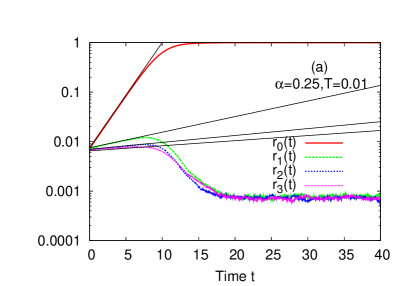
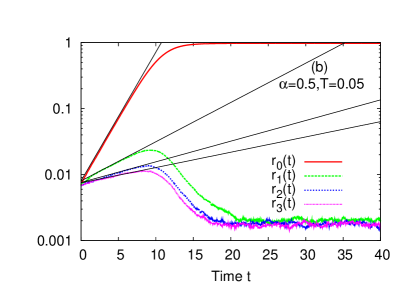
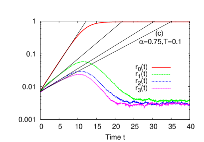
Figure 1: (Color online) Time evolution of the observables $r_{0}(t),r_{1}(t),r_{2}(t)$, and $r_{3}(t)$ starting from an initial state $\{\theta_{i}(0);i=1,2,...,N\}$, where the $\theta_{i}$’s are chosen uniformly in $[-\pi,\pi]$. Thus, initially, the system is in the uniform state (16). Here, the values of $\alpha$ and temperature $T$ are (a) $\alpha=0.25,T=0.01$, (b) $\alpha=0.5,T=0.05$, and (c) $\alpha=0.75,T=0.1$. From Table (1), it follows then that the Fourier modes $0,1,2,3$ in particular are linearly unstable. Consequently, $r_{0}(t),r_{1}(t),r_{2}(t)$, and $r_{3}(t)$ all grow in time from their initial values. However, the plots show that in the long-time limit, $r_{0}(t)$ attains a value very close to unity, while $r_{1}(t),r_{2}(t),r_{3}(t)$ all decay to a value very close to zero. The data in the plots are obtained from numerical simulations with $N=2^{14}$, and involve averaging over $100$ independent initial conditions and dynamical realizations. The straight lines show the initial exponential growth with rates given by $(T_{c,m}-T)$, where the values of $T_{c,m}$’s can be read off from Table 1. The agreement of the growth rates between theory and simulations is very good.

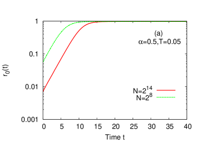
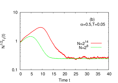
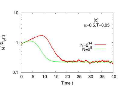
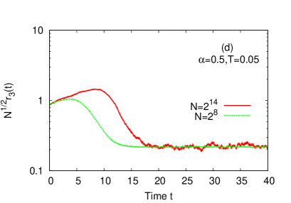
Figure 2: (Color online) Time evolution of the observables $r_{0}(t),r_{1}(t),r_{2}(t)$, and $r_{3}(t)$ starting from an initial state $\{\theta_{i}(0);i=1,2,...,N\}$, where the $\theta_{i}$’s are chosen uniformly in $[-\pi,\pi]$. Here, $\alpha=0.5$ and $T=0.05$. The plots show that in the long-time limit, $r_{0}(t)$ attains a value very close to unity and does not scale with the system size $N$, while $r_{1}(t),r_{2}(t),r_{3}(t)$ all decay to values that scale with $N$ as $1/\sqrt{N}$. The data involve averaging over $100$ independent initial conditions and dynamical realizations for $N=2^{14}$, and over $5000$ realizations for $N=2^{8}$.

In order to test the theoretical predictions in the limit $N\to\infty$ obtained in the preceding section regarding values of critical temperatures, and growth and decay of Fourier modes depending on the temperature, we performed extensive numerical simulations of the dynamics for large $N$. A standard procedure for simulations is to integrate the equation of motion (7) for each of the $N$ particles; this involves computing at every integration step a sum over $N$ terms for each particle, thus requiring a total computation time scaling with $N$ as $N^{2}$. In order to perform faster simulations, we adopted the algorithm discussed in Ref. Gupta:2012 to compute the sum in Eq. (7). This algorithm requires a total computation time that scales with $N$ as $N\ln N$. The equations of motion were integrated using a fourth-order Runge-Kutta algorithm with time step equal to $0.01$. The initial state of the system was chosen to be the uniform state (16), prepared by having each particle degree of freedom $\theta$ uniformly distributed in $[-\pi,\pi]$, independently of the others. We report here simulation results for system sizes $2^{14}$ and $2^{8}$.

In simulations, we monitor the observable

$$r_{m}(t)=\frac{1}{N}\Big{|}\sum_{j=1}^{N}e^{i(\theta_{j}+2\pi jm/N)}\Big{|};m=0,1,2,\ldots;$$ (29)

in particular, $r_{0}(t)$ does not contain any spatial dependence, and, thus, characterizes the mean-field mode. In the continuum limit, we have

$$r_{m}(t)=\Big{|}\int d\theta ds~{}e^{i(\theta+2\pi ms)}\rho(\theta;s,t)\Big{|}.$$ (30)

Starting at time $t=0$ from the uniform state such that $r_{m}(0)=0~{}\forall~{}m$, and at a temperature $T=0.01$ with $\alpha=0.25$, we expect from Table 1 that the Fourier modes $0,1,2,3$ in particular are linearly unstable. Consequently, $r_{0}(t),r_{1}(t),r_{2}(t),r_{3}(t)$ are expected to grow in time. Indeed, Fig. 1(a) displaying the simulation results for $r_{0}(t),r_{1}(t),r_{2}(t),r_{3}(t)$ does show that they all grow in time. However, in the long-time limit, we see that $r_{0}(t)$ saturates to a value very close to unity, while $r_{1}(t),r_{2}(t),r_{3}(t)$ all decay to a value very close to zero. By repeating simulations at different temperatures $T<1/2$ for different values of $\alpha<1$ (see Fig. 1(b),(c)), we have confirmed that $r_{0}(t)$ always saturates in the long-time limit to a non-zero stationary state value $r_{0}^{st}=r_{0}^{st}(T)$ that depends on the temperature, while $r_{m}(t)$’s, with $m\neq 0$, decay in the long-time limit to a stationary state value very close to zero. As shown in Fig. 2, the asymptotic value of $r_{0}(t)$ does not scale with the system size $N$, while that of $r_{m}(t)$ for $m\neq 0$ scales with the system size as $1/\sqrt{N}$, and hence approaches zero in the continuum limit $N\to\infty$. These observations suggest that for temperatures $T<1/2$ for all values of $\alpha<1$, the stationary state is characterized by a distribution $\rho_{0}$ which is non-uniform in $\theta$, but uniform in $s$, and may be obtained from Eq. (15) as:

$$\rho_{0}(\theta) \propto \exp\Big{[}\frac{\kappa(\alpha)}{T}\int d\theta^{\prime}ds^{\prime}\frac{\cos(\theta^{\prime}-\theta)}{(|s^{\prime}-s|_{c})^{\alpha}}\rho_{0}(\theta^{\prime})\Big{]}$$ (31)

$$= \exp\Big{[}\frac{1}{T}(m_{x}\cos\theta+m_{y}\sin\theta)\Big{]},$$

where

$$(m_{x},m_{y})\equiv\int_{0}^{2\pi}d\theta(\cos\theta,\sin\theta)\rho_{0}(\theta).$$ (32)

IV Non-uniform stationary state and dynamics of Fourier modes

Our observations regarding saturation of $r_{0}(t)$ and decay of $r_{m}(t)$’s, with $m\neq 0$, detailed in the preceding section, raise an immediate question: Can we show by performing a linear stability analysis of the state (31) at temperatures $T<1/2$ that all the modes of fluctuations decay in the long-time limit to zero, so that the state is linearly stable for all values of $\alpha<1$?

Before proceeding with the stability analysis, we note that our system has full rotational invariance in $\theta$ at each space point, so that in the following, we take $m_{y}=0$ and $0\leq m_{x}\leq 1$ without any loss of generality; then, we have

$$\rho_{0}(\theta) = A\exp\Big{[}\frac{1}{T}m_{x}\cos\theta\Big{]},$$ (33)

where $A$ is the normalization:

$$A=\frac{1}{\int_{0}^{2\pi}d\theta e^{\frac{m_{x}}{T}\cos\theta}}.$$ (34)

Note that the quantity $m_{x}$ is determined self-consistently by combining Eq. (33) with Eq. (32); one gets

$$m_{x}=\frac{I_{1}(m_{x}/T)}{I_{0}(m_{x}/T)},$$ (35)

where $I_{n}(x)$ is the modified Bessel function of order $n$:

$$I_{n}(x)=\frac{1}{2\pi}\int_{0}^{2\pi}d\theta~{}e^{x\cos\theta}\cos n\theta.$$ (36)

We thus have $A=\left[2\pi I_{0}(m_{x}/T)\right]^{-1}$.

To study the linear stability of the state (33), we write

$$\rho(\theta;s,t)=\rho_{0}(\theta)+\delta\rho(\theta;s,t);~{}~{}~{}~{}\delta\rho(\theta;s,t)\ll 1,$$ (37)

where we expand $\delta\rho(\theta;s,t)$ as

$$\delta\rho(\theta;s,t)=\sum_{m=-\infty}^{\infty}\widehat{\delta\rho}_{m}(\theta,t)e^{i2\pi ms}.$$ (38)

Using Eq. (38) in Eq. (14), we find that $\widehat{\delta\rho}_{m}(\theta,t)$ satisfies at its leading order the equation

$$\frac{\partial\widehat{\delta\rho}_{m}}{\partial t}=m_{x}\frac{\partial(\sin\theta~{}\widehat{\delta\rho}_{m})}{\partial\theta}+T\frac{\partial^{2}\widehat{\delta\rho}_{m}}{\partial\theta^{2}}$$

$$-\lambda_{m}(\alpha)\frac{\partial}{\partial\theta}\Big{(}\Big{[}\int d\theta^{\prime}\sin(\theta^{\prime}-\theta)\widehat{\delta\rho}_{m}(\theta^{\prime},t)\Big{]}\rho_{0}\Big{)},$$ (39)

where we have defined

$$\lambda_{m}(\alpha)\equiv\kappa(\alpha)\Lambda_{m}(\alpha).$$ (40)

The eigenfrequencies associated with the linear equation (39) can be studied by looking for solutions of the form

$$\widehat{\delta\rho}_{m}(\theta,t)=\widetilde{\delta\rho}_{m}(\theta,\omega)e^{i\omega t}.$$ (41)

Before studying the spectrum of the eigenfrequency $\omega$, it is instructive to analyze the explicit solution $\widetilde{\delta\rho}_{m}(\theta,0)$ corresponding to the neutral mode $\omega=0$. We find from Eq. (39) that $\widetilde{\delta\rho}_{m}(\theta,0)$ satisfies

$$m_{x}\sin\theta~{}\widetilde{\delta\rho}_{m}-\lambda_{m}(\alpha)\Big{(}\widetilde{m}_{y}\cos\theta-\widetilde{m}_{x}\sin\theta\Big{)}\rho_{0}$$

$$+T\frac{\partial\widetilde{\delta\rho}_{m}}{\partial\theta}=C,$$ (42)

where $C$ is a constant independent of $\theta$, and

$$(\widetilde{m}_{x},\widetilde{m}_{y})=\int d\theta(\cos\theta,\sin\theta)\widetilde{\delta\rho}_{m}(\theta,0).$$ (43)

Equation (42) has the solution

$$\widetilde{\delta\rho}_{m}(\theta,0) = \widetilde{\delta\rho}_{m}(0,0)e^{-\frac{m_{x}}{T}(1-\cos\theta)}$$ (44)

$$+\frac{C}{T}e^{\frac{m_{x}}{T}\cos\theta}\int_{0}^{\theta}d\theta^{\prime}e^{-\frac{m_{x}}{T}\cos\theta^{\prime}}$$

$$+\frac{A\lambda_{m}(\alpha)\widetilde{m}_{y}}{T}e^{\frac{m_{x}}{T}\cos\theta}\sin\theta$$

$$-\frac{A\lambda_{m}(\alpha)\widetilde{m}_{x}}{T}e^{\frac{m_{x}}{T}\cos\theta}(1-\cos\theta).$$

The periodicity condition $\widetilde{\delta\rho}_{m}(\theta+2\pi,0)=\widetilde{\delta\rho}_{m}(\theta,0)$ implies that $C=0$. Normalization of $\rho(\theta;s,t)$ for all times implies, using Eq. (37) and the fact that $\rho_{0}(\theta)$ is normalized, that $\int_{0}^{2\pi}d\theta~{}\widetilde{\delta\rho}_{m}(\theta,0)=0~{}\forall~{}m$. Then, from Eq. (44) with $C=0$, we get

$$\widetilde{\delta\rho}_{m}(0,0)\int_{0}^{2\pi}d\theta e^{-\frac{m_{x}}{T}(1-\cos\theta)}$$

$$=\frac{A\lambda_{m}(\alpha)\widetilde{m}_{x}}{T}\int_{0}^{2\pi}d\theta e^{\frac{m_{x}}{T}\cos\theta}(1-\cos\theta).$$ (45)

Using the above equation and Eq. (35) in Eq. (44) with $C=0$, we arrive at the following expression for $\widetilde{\delta\rho}_{m}(\theta,0)$:

$$\widetilde{\delta\rho}_{m}(\theta,0)$$

$$=\frac{A\lambda_{m}(\alpha)}{T}e^{\frac{m_{x}}{T}\cos\theta}\left[\widetilde{m}_{x}\left(\cos\theta-m_{x}\right)+\widetilde{m}_{y}\sin\theta\right].$$ (46)

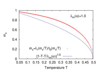
Figure 3: (Color online) Plot showing as a function of $T$ the values of $m_{x}$ that satisfy Eq. (35), and those that satisfy (49) at $\lambda_{m}(\alpha)=1$. The fact that the curves do not intersect at any $T$ in the range $0<T<1/2$ shows that in this range, the value of $m_{x}$ that solves Eq. (35) at a given $T$ does not satisfy Eq. (49).

The quantities $\widetilde{m}_{x,y}$ in Eq. (46) are determined self-consistently. They cannot both be equal to zero, as would have happened if $\widetilde{\delta\rho}_{m}(\theta,0)$ were a constant, but this is not possible as the integral of $\widetilde{\delta\rho}_{m}(\theta,0)$ from $0$ to $2\pi$ is required to vanish. Using Eqs. (43), (46), (34) and (35), we get the following two equations:

$$\widetilde{m}_{y}=\widetilde{m}_{y}\frac{\lambda_{m}(\alpha)}{m_{x}}\frac{I_{1}(m_{x}/T)}{I_{0}(m_{x}/T)},$$ (47)

$$\widetilde{m}_{x}=\widetilde{m}_{x}\frac{\lambda_{m}(\alpha)}{T}\left(1-T-m_{x}^{2}\right),$$ (48)

where $0<T<1/2$, and $m_{x}$ satisfies Eq. (35). Equation (47) is obviously satisfied for $\widetilde{m}_{y}=0$. If $\widetilde{m}_{y}\neq 0$, then, using Eq. (35), we see that Eq. (47) is an identity for $m=0$, while it has no solution for $m\neq 0$, which follows from the property that $\lambda_{m}(\alpha)<1$ for $m\neq 0$. Let us now analyze Eq. (48). It is satisfied for $\widetilde{m}_{x}=0$. If $\widetilde{m}_{x}\neq 0$, it gives

$$m_{x}=\sqrt{1-T-T/\lambda_{m}(\alpha)},$$ (49)

giving a relation between $m_{x}$ and $T$, which has to be satisfied together with Eq. (35). To check whether the two equations are consistent, note that $\lambda_{m}(\alpha)=\lambda_{-m}(\alpha)$ and that $\lambda_{m}(\alpha)\geq 0$ is a monotonically decreasing function of $|m|$, with $\lambda_{0}(\alpha)=1$ and $\lim_{m\to\pm\infty}\lambda_{m}(\alpha)=0$. Hence, to check the consistency, we have to consider in Eq. (49) any value for $\lambda_{m}(\alpha)$ between $0$ and $1$. Actually, when $\lambda_{m}(\alpha)<1$, Eq. (49) gives a real value for $m_{x}$ only for $T$ in the range $0<T<\frac{\lambda_{m}(\alpha)}{1+\lambda_{m}(\alpha)}$, which is smaller than the range $0<T<1/2$. In Fig. 3, we plot $m_{x}(T)$ as given by Eq. (49) for $\lambda_{m}(\alpha)=1$, and as given by solving the implicit equation (35). We see that the two curves do not intersect. This also implies that there cannot be any intersection for $\lambda_{m}(\alpha)<1$, since the right hand side of Eq. (49) decreases on decreasing $\lambda_{m}(\alpha)$. Thus, we conclude that Eq. (49) for $0<T<1/2$ is not solved by $m_{x}$ that satisfies Eq. (35). In summary, the two equations, (47) and (48), are not satisfied by $m_{x}$ given by Eq. (35), when $m\neq 0$. When $m=0$, there is only one solution, namely, $\widetilde{m}_{x}=0$, and $\widetilde{m}_{y}$ any non-zero value. For this solution, on using Eqs. (33) and (46), we have

$$\widetilde{\delta\rho}_{0}(\theta,0)=\frac{1}{T}\rho_{0}(\theta)\widetilde{m}_{y}\sin\theta,$$ (50)

which is just a perturbation of $\rho_{0}(\theta)$ that corresponds to a rotation in $\theta$ space of all the rotators of the system. It is therefore natural that it corresponds to a neutral mode.

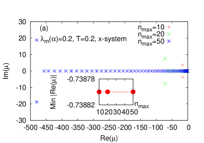
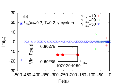
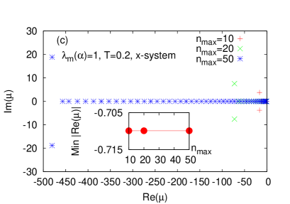
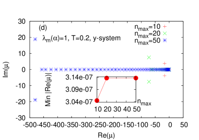
Figure 4: (Color online) Real and imaginary parts of the eigenvalues $\mu$ of the $x$-system, Eq. (53), and the $y$-system, Eq. (54), for a $m\neq 0$ mode such that $\lambda_{m}(\alpha)<1$ and for the $m=0$ mode such that $\lambda_{m}(\alpha)=1$. The temperature is $T=0.2$. The parameter $n_{max}$ denotes the order of truncation of the eigenvalue equations.

On the basis of the above discussion, we conclude that there is no temperature $T<1/2$ such that the $m$th mode of fluctuations, for any $m$, has a vanishing eigenfrequency, excepting for the trivial one for $m=0$ that corresponds to a state obtained by a rotation in $\theta$ space of all the rotators of the system. Thus, the $m$th mode either grows or decays in time at all temperatures $T<1/2$, corresponding to eigenfrequencies $\omega$ which have respectively a negative or a positive imaginary part.

In order to examine the entire spectrum of the eigenfrequency $\omega$, we use Eqs. (39) and (41), and the substitution $\mu\equiv i\omega$ to get the following equation for $\widetilde{\delta\rho}_{m}(\theta,\omega)$.

$$\mu\widetilde{\delta\rho}_{m}=m_{x}\frac{\partial(\sin\theta~{}\widetilde{\delta\rho}_{m})}{\partial\theta}+T\frac{\partial^{2}\widetilde{\delta\rho}_{m}}{\partial\theta^{2}}$$

$$-\lambda_{m}(\alpha)\frac{\partial}{\partial\theta}\Big{(}\Big{[}\int d\theta^{\prime}\sin(\theta^{\prime}-\theta)\widetilde{\delta\rho}_{m}(\theta^{\prime},\omega)\Big{]}\rho_{0}\Big{)}.$$ (51)

Let us define

$$(\widetilde{m}^{(n)}_{x},\widetilde{m}^{(n)}_{y})=\int d\theta(\cos n\theta,\sin n\theta)\widetilde{\delta\rho}_{m}(\theta,\omega),$$

(52)

$$m^{(n)}_{x}=\int d\theta\cos n\theta~{}\rho_{0}(\theta)=\frac{I_{n}(m_{x}/T)}{I_{0}(m_{x}/T)},$$

where we note that $m^{(1)}_{x}=m_{x}$. On multiplying Eq. (51) in turn by $\cos n\theta$ and $\sin n\theta$, integrating over $\theta$ from $0$ to $2\pi$, noting that $\rho_{0}$ is even in $\theta$, that $\widetilde{\delta\rho}_{m}(2\pi,\omega)=\widetilde{\delta\rho}_{m}(0,\omega)$, and that $\rho_{0}(2\pi)=\rho_{0}(0)$, we arrive at the following system of equations for $n\geq 1$:

$$\mu\widetilde{m}^{(n)}_{x} = \frac{1}{2}nm_{x}\Big{(}\widetilde{m}^{(n-1)}_{x}-\widetilde{m}^{(n+1)}_{x}\Big{)}-Tn^{2}\widetilde{m}^{(n)}_{x}$$ (53)

$$+\frac{1}{2}\lambda_{m}(\alpha)n\widetilde{m}^{(1)}_{x}\Big{(}m^{(n-1)}_{x}-m^{(n+1)}_{x}\Big{)},$$

$$\mu\widetilde{m}^{(n)}_{y} = \frac{1}{2}nm_{x}\Big{(}\widetilde{m}^{(n-1)}_{y}-\widetilde{m}^{(n+1)}_{y}\Big{)}-Tn^{2}\widetilde{m}^{(n)}_{y}$$ (54)

$$+\frac{1}{2}\lambda_{m}(\alpha)n\widetilde{m}^{(1)}_{y}\Big{(}m^{(n-1)}_{x}+m^{(n+1)}_{x}\Big{)},$$

where $\widetilde{m}^{(0)}_{x}=\widetilde{m}^{(0)}_{y}=0$, and $m^{(0)}_{x}=1$. The operators on the right-hand sides of the above equations being non-hermitian have in general both real and complex eigenvalues.

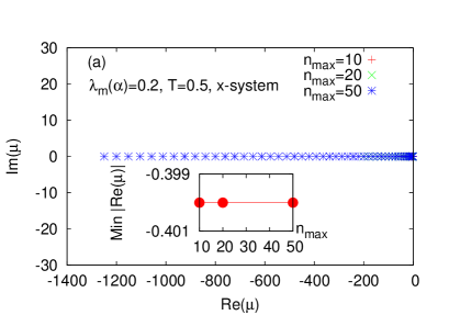
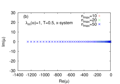
Figure 5: (Color online) Real and imaginary parts of the exact eigenvalues $\mu$ of the $x$-system, Eqs. (55) and (57), for a $m\neq 0$ mode such that $\lambda_{m}(\alpha)<1$ and for the $m=0$ mode such that $\lambda_{m}(\alpha)=1$. The temperature is $T=0.5$. The parameter $n_{max}$ denotes the order of truncation of the eigenvalue equations.

When $T<1/2$ and $m^{(n)}_{x}\neq 0$ for all $n\in\mathcal{N}$, then, combined with Eq. (35), the eigenvalues of the system of equations, (53) and (54), can be obtained numerically after truncating the equations to a finite value of $n$, say, $n_{max}$. As argued before on the basis of properties of $\lambda_{m}(\alpha)$, in order to probe the behavior of a $m\neq 0$ mode of fluctuations, it suffices to consider any real positive value $<1$ for $\lambda_{m}(\alpha)$, while for the $m=0$ mode, we have $\lambda_{m}(\alpha)=1$. The results for the eigenvalue spectrum of Eqs. (53) and (54) are shown in Fig. 4 for the temperature $T=0.2$.

When $T\geq 1/2$ and $m^{(n)}_{x}=0$ for all $n\in\mathcal{N}$, the eigenvalue equations, (53) and (54), simplify for $n\geq 2$ to

$$\mu\widetilde{m}^{(n)}_{x} = -Tn^{2}\widetilde{m}^{(n)}_{x},$$ (55)

$$\mu\widetilde{m}^{(n)}_{y} = -Tn^{2}\widetilde{m}^{(n)}_{y},$$ (56)

while for $n=1$, the equations are

$$\mu\widetilde{m}^{(1)}_{x} = -T\widetilde{m}^{(1)}_{x}+\frac{1}{2}\lambda_{m}(\alpha)\widetilde{m}^{(1)}_{x},$$ (57)

$$\mu\widetilde{m}^{(1)}_{y} = -T\widetilde{m}^{(1)}_{y}+\frac{1}{2}\lambda_{m}(\alpha)\widetilde{m}^{(1)}_{y}.$$ (58)

The system of equations, (55)-(58) is a set of independent equations, and may be solved quite easily to get the exact eigenvalues $\mu$; from the equations, it is clear that these eigenvalues are the same for the $x$ and the $y$-system. Of course, the number of eigenvalues depends on the value $n_{max}$ of $n$ at which the equations are truncated. In particular, for $\lambda_{m}(\alpha)=1$ and $T=1/2$, one finds the eigenvalue $\mu=0$. The results for the eigenvalue spectrum of Eqs. (55)-(58) are shown in Fig. 5 for the temperature $T=1/2$.

Let us first discuss the results displayed in Fig. 4. From the $m\neq 0$ mode results, displayed in panels (a) and (b), we see that the eigenvalues of the $x$- and the $y$-system are both real and complex, but the important thing to note is that the real eigenvalues are all negative while the complex ones have strictly negative real parts. In order to demonstrate the former fact, a zoom into the region near the zero of the $Re(\mu)$ axis, shown in the insets, illustrates that the eigenvalue closest to 0 of both the $x$- and the $y$-system has a negative real part, so that the remaining eigenvalues having larger real parts in magnitude are thus all negative. The insets also show that the eigenvalue with the smallest negative real part converges in magnitude on increasing the truncation order $n_{max}$. For higher $n_{max}$, only the number of eigenvalues increases; in particular, only the number of real eigenvalues with larger magnitude increases, while there is still only one complex eigenvalue which has the largest negative real part. Computing the eigenvalues for other $\lambda_{m}$’s and temperatures $T<1/2$, we find that the number of complex eigenvalues is always small (with the number increasing for smaller $\lambda_{m}$’s and $T$’s), and these eigenvalues always have large negative real parts. Since the $m$th mode of fluctuations has the time dependence $\sim e^{\mu t}$ (recall Eq. (41) and the definition of $\mu=i\omega$), and since all values for $\mu$ have strictly negative real parts, it follows that at temperatures $T<1/2$, the $m$th mode of fluctuations, with $m\neq 0$, decays in the long-time limit to zero. Figure 4, panel (c) shows that the behavior for the $m=0$ mode is very similar to that observed in panels (a) and (b) for $m\neq 0$, discussed above. Panel (d) also has the same general behavior, excepting that now the eigenvalue closest to the origin of the $Re(\mu)$ axis, shown in the inset as a function of $n_{max}$, is very slightly ($\sim 10^{-7}$) positive. Actually, this eigenvalue should be exactly zero, being the one corresponding to rotational invariance that we discussed earlier (see the discussion following Eq. (49)). In fact, using Eq. (50) in Eq. (52) to compute $\widetilde{m}^{(n)}_{y}$, and using it in Eq. (54), it may be checked that its right hand side is zero for any $n$, that is, the particular solution (50) gives $\mu=0$. The slight positive value is just a numerical artifact.

We now discuss the results displayed in Fig. 5. We show here only the eigenvalues of the $x$-system, since, as noted earlier, the $y$-system has exactly the same eigenvalue spectrum. From the $m\neq 0$ mode results, displayed in panel (a), we see that the eigenvalues are only real and negative, with no complex eigenvalue. The eigenvalue closest to the origin of the $Re(\mu)$ axis, shown in the inset as a function of $n_{max}$, dominates the behavior of the $m$th mode of fluctuations in time, thereby making it decay to zero in the long-time limit. From the $m=0$ mode results, displayed in panel (b), we see that the eigenvalues are real and negative. As already mentioned above, the eigenvalue closest to the origin is precisely zero, which makes the zero mode of fluctuations to neither grow nor decay at the temperature $T=1/2$.

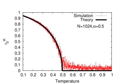
Figure 6: Plot showing $r_{0}^{st}$ as a function of temperature. The data are obtained by starting from the uniform state (16) at a high temperature $T=1$, and then changing adiabatically the temperature as a function of time $t$ as $T(t)=1-Rt$, where the rate $R$ is taken to be such that $R\tau_{st}\ll 1$, with $\tau_{st}$ being the time to reach stationary state at a fixed temperature. The condition $R\tau_{st}\ll 1$ ensures that between two successive values of $T$, the system gets enough time to attain stationarity. For a system of size $N$, taking $\tau_{st}=N^{2}dt$, where $dt$ is the numerical integration timestep, we take $R=0.1/N^{2}dt$.

Based on results discussed in this section and in section II, we conclude that the linearly stable stationary state of the dynamics (7) in the $N\to\infty$ limit is a state uniform in space but non-uniform in $\theta$ when the temperature is less that $1/2$. On tuning the temperature to a value larger than $1/2$, the stationary state becomes uniform in $\theta$. Thus, our linear stability analysis in the limit $N\to\infty$ allows us to predict that the system undergoes a transition at the temperature $T=T_{c,0}=1/2$. Indeed, simulation results shown in Fig. 6 for $r_{0}^{st}$ suggests a continuous phase transition as a function of temperature, where we also show the theoretical curve for $r_{0}^{st}$ obtained by combining Eq. (30) with Eq. (33) to give for $T<1/2$ the result

$$r_{0}^{st}=\frac{I_{1}(m_{x}/T)}{I_{0}(m_{x}/T)}=m_{x};$$ (59)

for $T>1/2$, on using Eq. (16), one has

$$r_{0}^{st}=0.$$ (60)

Exactly at $T=1/2$, we have $r_{0}^{st}=0$.

V Conclusions and perspectives

In this paper, we considered a paradigmatic long-range interacting model of particles residing on the sites of a one-dimensional periodic lattice. Each particle has an internal degree of freedom $\theta$ which is coupled to those of other particles with an attractive $XY$-like interaction $\sim-\cos(\theta_{i}-\theta_{j})$ between the $i$th and $j$th particles, with the coupling strength decaying with the interparticle separation $r$ as $1/r^{\alpha}$;  $0<\alpha<1$. We considered the overdamped dynamics within a canonical ensemble of this so-called $\alpha$-HMF model. We studied the model numerically, and also analytically in the continuum limit through the Fokker-Planck equation for the evolution of the local density of particles.

The Fokker-Planck equation allows a stationary state which is uniform in both $\theta$ and space $s$ of the lattice. A linear stability analysis of such a state shows that it is stable above the temperature $T=1/2$. Below this temperature, when it is unstable, numerics as well as the linear stability analysis show that different spatial Fourier modes of fluctuations (the number of which depends on the temperature) grow exponentially in time with different rates. However, our numerical simulations also show that all the non-zero Fourier modes decay at long times to zero. By contrast, the zero mode (the “mean-field” mode) grows and reaches a non-zero value, corresponding to a non-uniform stationary state, i.e. a state which is non-uniform in $\theta$, but uniform in $s$.

On the basis of our investigations, it appears that both for temperatures below and above $T=1/2$, the state which is uniform in space acts as a global attractor of all possible stationary states of the $\alpha$-HMF model. The state is the same as the equilibrium state of the mean-field version of the model, the HMF model. For temperatures below $1/2$, the late-time damping of the unstable non-zero modes after their initial growth is an interesting and unexpected phenomenon. For such temperatures, by developing a linear stability analysis around the non-uniform state, we showed that all fluctuations around that state decay in time, thereby stabilizing the state; describing analytically the complete evolution of the unstable non-zero modes, from their initial growth in time to their late-time decay, thereby leading to the convergence to the non-uniform state remains an interesting challenging problem.

The model we studied may be related to the Kuramoto model in the field of non-linear dynamical systems Kuramoto:1984 ; Strogatz:2000 ; Acebron:2005 . Interpreting each of the $N$ particles of our system to be a phase-only oscillator with phase $\theta_{i}$, the equation of motion (7) may be looked upon as the one governing the time evolution of the phase of the $i$th oscillator, in the presence of thermal noise. On considering $\alpha=0$ in Eq. (7), the model in the absence of thermal noise is a particular limit of the Kuramoto model in which each oscillator has the same intrinsic frequency of oscillation. In the presence of thermal noise, Eq. (7) with $\alpha=0$ is the generalization of the Kuramoto model considered in Ref. Sakaguchi:1988 . On considering $\alpha\neq 0$, and attributing to each oscillator an intrinsic frequency sampled from a distribution, the model in the absence of thermal noise has been considered in Rogers:1996 ; Chowdhury:2010 ; Uchida:2011 ; Gupta:2012 . In particular, a mean-field dominance similar to the one observed in this work has been seen in numerics in Ref. Gupta:2012 . It remains an open problem to relate this dominance in these two scenarios.

VI Acknowledgments

S. G. and S. R. acknowledge the contract ANR-10-CEXC-010-01 for support. The motivation for this work arose from discussions in two workshops held at the Korea Institute for Advanced Study (KIAS), Seoul, and at the Centre Blaise Pascal, ENS-Lyon in July and August, 2012, respectively. S. G. and S. R. thank KIAS for hospitality during their mutual visit in July, 2012. A. C. acknowledges ENS-Lyon for hospitality during some stages of the work presented in this paper. We acknowledge useful discussions with David Mukamel and Hyunggyu Park.

References

- (1) A. Campa, T. Dauxois, and S. Ruffo, Phys. Rep. 480, 57 (2009).
- (2) Long-Range Interacting Systems, edited by T. Dauxois, S. Ruffo, and L. F. Cugliandolo (Oxford University Press, New York, 2010).
- (3) F. Bouchet, S. Gupta, and D. Mukamel, Physica A 389, 4389 (2010).
- (4) P. H. Chavanis, Int. J. Mod. Phys. B 20, 3113 (2006).
- (5) D. F. Escande, in Long-Range Interacting Systems, edited by T. Dauxois, S. Ruffo, and L. F. Cugliandolo (Oxford University Press, New York, 2010).
- (6) F. Bouchet and A. Venaille, Phys. Rep. 515, 227 (2012).
- (7) S. T. Bramwell, in Long-Range Interacting Systems, edited by T. Dauxois, S. Ruffo, and L. F. Cugliandolo (Oxford University Press, New York, 2010).
- (8) J. Barré, D. Mukamel, and S. Ruffo, Phys. Rev. Lett. 87, 030601 (2001).
- (9) D. Mukamel, S. Ruffo, and N. Schreiber, Phys. Rev. Lett. 95, 240604 (2005); F. Bouchet, T. Dauxois, D. Mukamel, and S. Ruffo, Phys. Rev. E 77, 011125 (2008).
- (10) Y. Y. Yamaguchi, J. Barré, F. Bouchet, T. Dauxois, and S. Ruffo, Physica A 337, 36 (2004).
- (11) M. Antoni and S. Ruffo, Phys. Rev. E 52, 2361 (1995).
- (12) S. Gupta and D. Mukamel, J. Stat. Mech. Theory Exp. P03015 (2011).
- (13) Y. Levin, R. Pakter, and T. N. Teles, Phys. Rev. Lett. 100, 040604 (2008).
- (14) M. Joyce and T. Worrakitpoonpon, Phys. Rev. E 84, 011139 (2011).
- (15) T. N. Teles, Y. Levin, R. Pakter, and F. B. Rizzato, J. Stat. Mech. Theory Exp. P05007 (2010).
- (16) J. Binney and S. Tremaine, Galactic Dynamics (Princeton University Press, Princeton, 2008), Chapter 2.
- (17) C. Anteneodo and C. Tsallis, Phys. Rev. Lett. 80, 5313 (1998); F. Tamarit and C. Anteneodo, Phys. Rev. Lett. 84, 208 (2000).
- (18) A. Campa, A. Giansanti, and D. Moroni, Phys. Rev. E 62, 303 (2000); A. Campa, A. Giansanti, and D. Moroni, J. Phys. A 36, 6897 (2003).
- (19) M.-C. Firpo and S. Ruffo, J. Phys. A 34 L511 (2001).
- (20) C. Anteneodo and R. O. Vallejos, Phys. Rev. E 65 016210 (2001).
- (21) A. Campa, A. Giansanti, and D. Moroni, Physica A 305 137 (2002).
- (22) S. Goto and Y. Y. Yamaguchi, Physica A 354, 312 (2005).
- (23) J.A. Acebrón and R. Spigler, Phys. Rev. Lett. 81, 2229 (1998); J.A. Acebrón, L.L. Bonilla, and R. Spigler, Phys. Rev. E 62, 3437 (2000).
- (24) P. H. Chavanis, J. Vatteville, and F. Bouchet, Eur. Phys. J. B 46, 61 (2005).
- (25) R. Bachelard, T. Dauxois, G. De Ninno, S. Ruffo, and F. Staniscia, Phys. Rev. E 83, 061132 (2011).
- (26) S. Gupta, M. G. Potters, and S. Ruffo, Phys. Rev. E 85, 066201 (2012).
- (27) Y. Kuramoto, Chemical Oscillations, Waves and Turbulence (Springer, Berlin, 1984).
- (28) S. H. Strogatz, Physica D 143, 1 (2000).
- (29) J. A. Acebrón, L. L. Bonilla, C. J. Pérez Vicente, F. Ritort, and R. Spigler, Rev. Mod. Phys. 77, 137 (2005).
- (30) H. Sakaguchi, Prog. Theor. Phys. 79, 39 (1988).
- (31) J. L. Rogers and L. T. Wille, Phys. Rev. E 54, R2193 (1996).
- (32) D. Chowdhury and M. C. Cross, Phys. Rev. E 82, 016205 (2010).
- (33) N. Uchida, Phys. Rev. Lett. 106, 064101 (2011).