Cosmological constraints on polytropic gas model

Abstract

We study the polytropic gas scenario as the unification of dark matter and dark energy. We fit the model parameters by using the latest observational data including type Ia supernovae, baryon acoustic oscillation, cosmic microwave background, and Hubble parameter data. At 68.3% and 95.4% confidence levels, we find the best fit values of the model parameters as $\tilde{K}=0.742_{-0.024}^{+0.024}(1\sigma)_{-0.049}^{+0.048}(2\sigma)$ and $n=-1.05_{-0.08}^{+0.08}(1\sigma)_{-0.16}^{+0.15}(2\sigma)$. Using the best fit values of the model, we obtain the evolutionary behaviors of the equation of state parameters of the polytropic gas model and dark energy, the deceleration parameter of the universe as well as the dimensionless density parameters of dark matter and dark energy. We conclude that in this model, the universe starts from the matter dominated epoch and approaches a de Sitter phase at late times, as expected. Also the universe begins to accelerate at redshift $z_{\rm t}=0.74$. Furthermore in contrary to the $\Lambda$CDM model, the cosmic coincidence problem is solved naturally in the polytropic gas scenario.

PACS numbers: 95.35.+d, 95.36.+x
Keywords: Dark matter, Dark energy

1 Introduction

Various cosmological observations, including the type Ia supernovae (SNeIa) [1], cosmic microwave background (CMB) [2] and baryon acoustic oscillation (BAO) [3], etc., have revealed that the current expansion of the universe is accelerating and it entered this accelerating phase only in the near past. A new energy component with negative pressure called dark energy (DE) is needed to explain this acceleration expansion within the framework of general relativity (GR). The simplest and most appealing candidate for DE is the $\Lambda$ cold dark matter ($\Lambda$CDM) model, in which the cosmological constant $\Lambda$ plays a role of DE in GR. This model is in general agreement with current astronomical observations, but has difficulties in reconciling the small observational value of DE density to that coming from quantum field theories. This is called the cosmological constant problem [4]. Therefore, a number of models for DE to explain the current acceleration without the cosmological constant has been proposed, such as quintessence [5], phantom [6], K-essence [7], tachyon [8], quintom [9]; as well as the Chaplygin gas [10] and the generalized Chaplygin gas [11], the holographic DE [12], the new agegraphic DE [13], the Ricci DE [14], and so on.

One of interesting DE models is the polytropic gas which was proposed to explain the accelerated expansion of the universe [15, 16, 17]. It was shown that the polytropic gas model in the presence of interaction with DM can behave as phantom type DE [16]. It was pointed out that a polytropic scalar field can be reconstructed according to the evolutionary behaviors of the holographic [18] and new agegraphic [19] DE densities. The validity of the generalized second law of gravitational thermodynamics was examined for the polytropic gas model in [20]. Different modified gravity models including $f(T)$-gravity [21] and $f(R)$-gravity [22] were reconstructed according to the polytropic gas equation of state. The polytropic tachyon, K-essence and dilaton scalar field models were studied in [23]. In [24], the polytropic gas model was investigated from the viewpoint of statefinder diagnostic tool and $w-w^{\prime}$ analysis.

In the present work, our main aim is to fit the polytropic gas model and give the constraints on model parameters, with current observational data including SNeIa, CMB, BAO and observational Hubble data (OHD), filling in the gap existing in the literature. To do so, in section 2, we briefly review the polytropic gas model as unified picture of DM and DE in a spatially flat Friedmann-Robertson-Walker (FRW) universe. In section 3, we consider the cosmological constraints on the polytropic gas model by using the latest observational data. In section 4, we give numerical results. Section 5 is devoted to conclusions.

2 Polytropic gas model

For a polytropic gas model, the energy density $\rho_{\rm pol}$ and pressure $p_{\rm pol}$ satisfy the equation of state (EoS) [17]

$$p_{\rm pol}=-K\rho_{\rm pol}^{1+\frac{1}{n}},$$ (1)

where $K>0$ and the polytropic index $n$ are two constants of the model.

Here, we consider a spatially flat FRW universe containing only the polytropic fluid and baryonic matter. We ignore the contribution of radiation, as expected from the observations [25]. In the framework of the standard FRW cosmology, the first Friedmann equation reads

$$H^{2}=\frac{8\pi G}{3}(\rho_{\rm pol}+\rho_{\rm bm}),$$ (2)

where $H=\dot{a}/a$ is the Hubble parameter. Also $\rho_{\rm pol}$ and $\rho_{\rm bm}$ denote the energy densities of the polytropic and pressureless baryonic matter ($p_{\rm bm}=0$), respectively, which satisfy the following energy conservation laws

$$\dot{\rho}_{\rm pol}+3H(\rho_{\rm pol}+p_{\rm pol})=0,$$ (3)

$$\dot{\rho}_{\rm bm}+3H\rho_{\rm bm}=0.$$ (4)

Using the dimensionless density parameters

$$\Omega_{\rm pol}=\frac{\rho_{\rm pol}}{\rho_{\rm cr}}=\frac{8\pi G\rho_{\rm pol}}{3H^{2}},~{}~{}~{}\Omega_{\rm bm}=\frac{\rho_{\rm bm}}{\rho_{\rm cr}}=\frac{8\pi G\rho_{\rm bm}}{3H^{2}},$$ (5)

the Friedmann equation (2) is rewritten as follows

$$1=\Omega_{\rm pol}+\Omega_{\rm bm}.$$ (6)

Substituting Eq. (1) into (2) gives the evolution of the polytropic gas energy density in terms of redshift $z=\frac{1}{a}-1$ as

$$\rho_{\rm pol}=\rho_{\rm pol_{0}}\Big{[}\tilde{K}+(1-\tilde{K})(1+z)^{-3/n}\Big{]}^{-n},$$ (7)

where

$$\tilde{K}=\rho_{\rm pol_{0}}^{1/n}K,$$ (8)

and $\rm{\rho_{\rm pol_{0}}}$ is the polytropic energy density at present time. Also Eq. (4) gives

$$\rho_{\rm bm}=\rho_{\rm bm_{0}}(1+z)^{3}.$$ (9)

It is worth to note that the polytropic gas energy density (7) offers a unified picture of DM and DE. Because it smoothly interpolates between a non-relativistic matter phase, $\rho_{\rm pol}\propto(1+z)^{3}$, in the past and a negative-pressure DE regime, $\rho_{\rm pol}=-p_{\rm pol}$, at late time ($z\rightarrow-1$). Therefore, within the framework of unified DM-DE (UDME) scenario one can rewrite the polytropic gas energy density as

$$\rho_{\rm pol}=\rho_{\rm dm}+\rho_{\rm de},$$

$$p_{\rm pol}=p_{\rm de},$$ (10)

where the DM is a pressureless matter ($p_{\rm dm}=0$). Using Eqs. (1) and (7) one can obtain the EoS parameter $\omega_{\rm pol}$ of the polytropic gas model as

$$\omega_{\rm pol}(z)=\frac{p_{\rm pol}}{\rho_{\rm pol}}=-\frac{\tilde{K}}{\tilde{K}+(1-\tilde{K})\left(1+z\right)^{-3/n}}.$$ (11)

With the help of Eqs. (3), (4), (7) and (10), the energy densities of DM and DE evolve as follows

$$\rho_{\rm dm}=\rho_{\rm dm_{0}}(1+z)^{3},$$ (12)

$$\rho_{\rm de}=\rho_{\rm pol_{0}}\Big{[}\tilde{K}+(1-\tilde{K})(1+z)^{-3/n}\Big{]}^{-n}-\rho_{\rm dm_{0}}(1+z)^{3}.$$ (13)

Using Eqs. (1), (5) and (13) the EoS parameter of DE reads

$$\omega_{\rm de}(z)=\frac{p_{\rm de}}{\rho_{\rm de}}=\frac{-\tilde{K}(1-\Omega_{\rm bm_{0}})\Big{[}\tilde{K}+(1-\tilde{K})(1+z)^{-3/n}\Big{]}^{-1-n}}{(1-\Omega_{\rm bm_{0}})\Big{[}\tilde{K}+(1-\tilde{K})(1+z)^{-3/n}\Big{]}^{-n}-\Omega_{\rm dm_{0}}(1+z)^{3}}.$$ (14)

With the help of Eqs. (7) and (9) and using (5), the first Friedmann equation (2) takes the form

$$H^{2}(z,\textbf{p})=H_{0}^{2}\left\{(1-\Omega_{\rm bm_{0}})\Big{[}\tilde{K}+(1-\tilde{K})(1+z)^{-3/n}\Big{]}^{-n}+\Omega_{\rm bm_{0}}(1+z)^{3}\right\},$$ (15)

where $H_{0}=70.2\pm 1.4~{}\rm km~{}s^{-1}~{}Mpc^{-1}~{}(68\%~{}\rm CL)$ and $\Omega_{\rm bm_{0}}=\frac{8\pi G\rho_{\rm bm_{0}}}{3H_{0}^{2}}=0.0458\pm 0.0016~{}(68\%~{}\rm CL)$ are the present Hubble constant and the present value of the dimensionless BM density, respectively, which have been updated in the 7-year WMAP (WMAP7) data [25]. Also p indicate model parameters including $\tilde{K}$ and $n$. Thus, throughout this work we fix the Hubble and the baryon density parameters at $H_{0}=70.2$ and $\Omega_{\rm bm_{0}}=0.0458$. With $H_{0}$ and $\Omega_{\rm bm_{0}}$ being determined by independent measurements, in the next section we will use the cosmic observations to constrain the polytropic gas model parameters ($\tilde{K},n$).

For completeness, we give the deceleration parameter

$$q=-1-\frac{\dot{H}}{H^{2}},$$ (16)

which combined with the EoS and the dimensionless density parameters form a set of useful parameters for the description of the astrophysical observations. Using Eq. (15) the deceleration parameter (16) can be obtained as

$$q(z)=\frac{1}{2}\frac{\Omega_{\rm bm_{0}}(1+z)^{3}+(3\omega_{\rm pol}+1)(1-\Omega_{\rm bm_{0}})\left[\tilde{K}+(1-\tilde{K})(1+z)^{-3/n}\right]^{-n}}{\Omega_{\rm bm_{0}}(1+z)^{3}+(1-\Omega_{\rm bm_{0}})\left[\tilde{K}+(1-\tilde{K})(1+z)^{-3/n}\right]^{-n}}.$$ (17)

3 Observational constraints

Here, we fit the free parameters of the polytropic gas model (1) by using the recent observational data including SNeIa, BAO, CMB and OHD.

For the SNeIa data, we use the currently largest Union2.1 compilation [26] that contains a total of 580 SNeIa, which is an updated version of the Union2 compilation [27]. Cosmological constraints from SNeIa data are obtained through the distance modulus $\mu(z)$. The theoretical distance modulus is defined as [28, 29]

$$\mu_{\rm th}(z)=5\log_{10}D_{\rm L}(z)+\mu_{0},$$ (18)

where $\mu_{0}=42.38-5\log_{10}h$ and $h$ is the Hubble constant $H_{0}$ in units of $100~{}\rm{km~{}s^{-1}~{}Mpc^{-1}}$. Also the Hubble-free luminosity distance $D_{\rm L}(z)$ for the flat universe is given by

$$D_{\rm L}(z)=(1+z)\int_{0}^{z}\frac{dz^{\prime}}{E(z^{\prime};\textbf{p})},$$ (19)

with p the model parameters and $E(z;\textbf{p})=H(z;\textbf{p})/H_{0}$.

For using SNeIa data, theoretical model parameters are determined by minimizing the quantity [28, 29]

$$\tilde{\chi}_{\rm SN}^{2}=A-\frac{B^{2}}{C},$$ (20)

where

$$A=\sum_{\rm i=1}^{580}[\mu_{\rm obs}(z_{\rm i})-\mu_{\rm th}(z_{\rm i})]^{2}/\sigma_{\rm i}^{2},$$ (21)

$$B=\sum_{\rm i=1}^{580}[\mu_{\rm obs}(z_{\rm i})-\mu_{\rm th}(z_{\rm i})]/\sigma_{\rm i}^{2},$$ (22)

$$C=\sum_{\rm i=1}^{580}1/\sigma_{\rm i}^{2},$$ (23)

and $\sigma_{\rm i}$ stands for the $1\sigma$ uncertainty associated to the $i$th data point.

Next, we add the data from the observation of acoustic signatures in the large scale clustering of galaxies. Using the BAO data, one can minimize the $\chi_{\rm BAO}^{2}$ defined as [30, 3],

$$\chi_{\rm BAO}^{2}=\frac{\left[A_{\rm obs}-A_{\rm th}\right]^{2}}{\sigma_{A}^{2}},$$ (24)

where

$$A_{\rm th}=\sqrt{\Omega_{\rm m_{0}}}~{}E(z_{\rm b};\textbf{p})^{-1/3}\left[\frac{1}{z_{\rm b}}\int_{0}^{z_{\rm b}}\frac{dz^{\prime}}{E(z^{\prime};\textbf{p})}\right]^{2/3},$$ (25)

is the theoretical distance parameter and $z_{\rm b}=0.35$ is the redshift of luminous red galaxies sample of the Sloan Digital Sky Survey (SDSS). Here $A_{\rm obs}=0.469(n_{s}/0.98)^{-0.35}\pm 0.017$ is measured from the SDSS data [3] and the scalar spectral index $n_{s}$ is taken to be 0.968 [25].

Since the SNeIa and BAO data contain information about the universe at relatively low redshifts, we will include the CMB shift information by using the WMAP7 data [25] to probe the entire expansion history up to the last scattering surface. The shift parameter $R$ of the CMB is defined as [31, 32]

$$R_{\rm th}=\sqrt{\Omega_{\rm m_{0}}}\int_{0}^{z_{\rm rec}}\frac{dz^{\prime}}{E(z^{\prime};\textbf{p})},$$ (26)

where $z_{\rm rec}\simeq 1091.3$ is the redshift at the recombination epoch [25]. Also $\Omega_{\rm m_{0}}$ is the effective matter density parameter defined as

$$\Omega_{\rm m_{0}}=\Omega_{\rm bm_{0}}+(1-\Omega_{\rm bm_{0}})(1-\tilde{K})^{-n}.$$ (27)

This expression for $\Omega_{\rm m_{0}}$, is an estimate of the “matter” component of the polytropic gas fluid with the baryon density. The $\chi^{2}$ from the CMB constraint is given by

$$\chi_{\rm CMB}^{2}=\frac{\left[R_{\rm obs}-R_{\rm th}\right]^{2}}{\sigma_{R}^{2}},$$ (28)

where the observational value of $R_{\rm obs}$ has been updated to $1.725\pm 0.018$ from the WMAP7 data [25].

Finally, we further add the data from the observational Hubble parameter. The Hubble parameter is related to redshift with

$$H(z)=-\frac{1}{1+z}\frac{{\rm d}z}{{\rm d}t},$$ (29)

so if ${\rm d}z/{\rm d}t$ is known, $H(z)$ is obtained directly [33]. The best fit values of the model parameters from OHD can be determined by minimizing [34]

$$\chi_{\rm OHD}^{2}=\sum_{\rm i=1}^{12}\frac{\left[H_{\rm obs}(z_{\rm i})-H_{\rm th}(z_{\rm i},\textbf{p})\right]^{2}}{\sigma_{\rm i}^{2}},$$ (30)

where $H_{\rm th}$ is the theoretical value of the Hubble parameter and $H_{\rm obs}$ is the observed value. Table 1 shows the observational Hubble data containing the nine data from [35] and three additional data, in bold face, from [36].

As the relative likelihood function is defined by ${\mathcal{L}}=e^{-(\chi^{2}_{\rm total}-\chi^{2}_{\rm min})/2}$ [37], the best fit value of the model parameters follows from minimizing the sum

$$\chi_{\rm total}^{2}=\tilde{\chi}_{\rm SN}^{2}+\chi_{\rm BAO}^{2}+\chi_{\rm CMB}^{2}+\chi_{\rm OHD}^{2}.$$ (31)

4 Numerical results

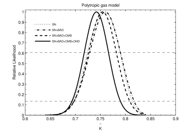
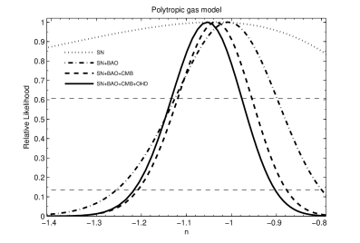
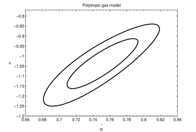
The best fit values and errors of the polytropic gas model parameters ($\tilde{K},n$) are summarized in Table 2, where we also list the best fit results of the $\Lambda$CDM model for comparison. At $1\sigma~{}(68.3\%)$ and $2\sigma~{}(95.4\%)$ confidence levels (CLs), we obtain the best fit values $\tilde{K}=0.742_{-0.024}^{+0.024}(1\sigma)_{-0.049}^{+0.048}(2\sigma)$ and $n=-1.05_{-0.08}^{+0.08}(1\sigma)_{-0.16}^{+0.15}(2\sigma)$ for the full data sets including SNeIa+BAO+CMB+OHD. The total $\chi^{2}$ of the best fit values of the polytropic gas model is $\chi_{\rm min}^{2}=573.089$ for the full data sets with $dof~{}(\rm degree~{}of~{}freedom)=594$. The reduced $\chi^{2}=\chi_{\rm min}^{2}/dof$ is $0.965$, which is acceptable. The obtained $\chi_{\rm min}^{2}$ is slightly smaller than the one for the $\Lambda$CDM model, $\chi_{\Lambda\rm CDM}^{2}=573.552$, for the same data sets. The marginalized relative likelihood functions ${\mathcal{L}}(\tilde{K})$ and ${\mathcal{L}}(n)$ are shown in Figs. 1 and 2, respectively. Considering only the SNeIa data, the degeneracy between the model parameters is considerable, but using the combined data this degeneracy is dropped in different ranges of redshift. Figure 3 shows the constraint on the polytropic gas parameter space $n-\tilde{K}$ at $1\sigma$ and $2\sigma$ CLs, using the full data sets.

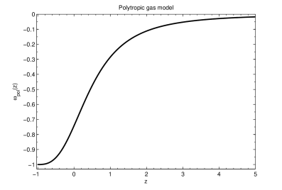
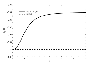
The variations of the EoS parameters of the polytropic gas model $\omega_{\rm pol}$ and DE $\omega_{\rm de}$ with the best fit values of the model are plotted in Figs. 4 and 5, respectively. Figure 4 presents that $\omega_{\rm pol}$ at early ($z>>1$) and late ($z\rightarrow-1$) times behave like the EoS parameters of the matter ($\omega_{\rm pol}=0$) and the cosmological constant ($\omega_{\rm pol}=-1$), respectively. This shows that in the polytropic gas scenario, the DM and DE can be unified. Figure 5 shows that $\omega_{\rm de}$ varies from $\omega_{\rm de}>-1$ to $\omega_{\rm de}=-1$, which is similar to the freezing quintessence model [38]. The current best fit value of the EoS parameter of the DE in the polytropic gas model is obtained as $\omega_{\rm de_{0}}=-0.98$ which is in good agreement with the recent observational result $\omega_{\rm de_{0}}=-0.93\pm 0.13~{}(68\%~{}\rm CL)$ deduced from the WMAP7 data [25].

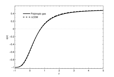
In Fig. 6, we plot the evolutionary behavior of the deceleration parameter of the universe with the best fit values of the polytropic gas model, Eq. (17), and the $\Lambda$CDM model. Figure 6 shows that very similar to the $\Lambda$CDM model the universe transits from an early matter dominant regime, i.e. $q=0.5$, to the de Sitter phase, i.e. $q=-1$, in the future, as expected. The accelerating expansion begins at transition redshift $z_{\rm t}=0.74$, which is earlier than what the $\Lambda$CDM model predicts, $z_{\rm t}^{\Lambda\rm CDM}=0.72$. The current best fit value of the deceleration parameter in the polytropic gas model is obtained as $q_{0}=-0.56$ which indicates the expansion rhythm of the current universe. This is in good agreement with the recent observational constraint $q_{0}=-0.43_{-0.17}^{+0.13}~{}(68\%~{}\rm CL)$ obtained by the cosmography [39].

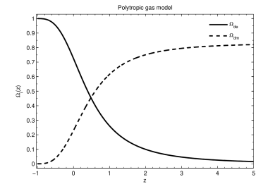
In Fig. 7, we plot the evolutionary behaviors of the energy density parameters of DM, $\Omega_{\rm dm}=\frac{8\pi G\rho_{\rm dm}}{3H^{2}}$, and DE, $\Omega_{\rm de}=\frac{8\pi G\rho_{\rm de}}{3H^{2}}$, with the best fit values of the polytropic gas model using the full data sets. Figure 7 shows that $\Omega_{\rm dm}$ and $\Omega_{\rm de}$ decreases and increases, respectively, during history of the universe. We also obtain $\Omega_{\rm dm_{0}}=0.229$ and $\Omega_{\rm de_{0}}=0.725$ as the current best fit values. These are in exact agreement with the latest observational results $\Omega_{\rm dm_{0}}=0.229\pm 0.015~{}(68\%~{}\rm CL)$ and $\Omega_{\rm de_{0}}=0.725\pm 0.016~{}(68\%~{}\rm CL)$ deduced from the WMAP7 data [25]. We also get $\Omega_{\rm de_{0}}/\Omega_{\rm dm_{0}}=3.166\simeq{\mathcal{O}}(1)$. This shows that in contrary to the $\Lambda$CDM model, the cosmic coincidence problem, namely why the ratio of the DE and DM densities is of order unity today, is solved naturally in the polytropic gas scenario.

5 Conclusions

Using the latest observational data from SNeIa, BAO, CMB and OHD, we fitted the parameters of the polytropic gas model as the unification of DM and DE. We obtained the constraint results of polytropic gas model parameters, $\tilde{K}=0.742_{-0.024}^{+0.024}(1\sigma)_{-0.049}^{+0.048}(2\sigma)$ and $n=-1.05_{-0.08}^{+0.08}(1\sigma)_{-0.16}^{+0.15}(2\sigma)$ for the full data sets. The minimal $\chi^{2}$ gives $\chi_{\rm min}^{2}=573.089$ with $dof=594$. The reduced $\chi^{2}$ equals to $0.965$ which is acceptable. The $\chi_{\rm min}^{2}$ is slightly smaller than the one for the $\Lambda$CDM model, $\chi_{\Lambda\rm CDM}^{2}=573.552$, for the same data sets.

Using the best fit values of the polytropic gas model parameters, we also studied the evolutionary behaviors of the EoS parameters of polytropic gas model and DE, the deceleration parameter of the universe as well as the DM and DE dimensionless density parameters. Our numerical results show the following.

(i) The evolutionary behavior of the EoS parameter $\omega_{\rm pol}$ of the polytropic gas model shows that the universe transits from an early matter dominated phase, i.e. $\omega_{\rm pol}=0$, to the $\Lambda$CDM model, i.e. $\omega_{\rm pol}=-1$, in the future, as expected. This confirms that the polytropic gas model plays the role of a unified model for DM and DE.

(ii) The EoS parameter $\omega_{\rm de}$ of DE in the polytropic gas scenario varies from $\omega_{\rm de}>-1$ to $\omega_{\rm de}=-1$ like a freezing quintessence model. The present value of $\omega_{\rm de_{0}}=-0.98$ is in good agreement with the result of WMAP7.

(iii) The variation of the deceleration parameter $q$ shows that the universe transits from an early matter dominant epoch, i.e. $q=0.5$, to the de Sitter era, i.e. $q=-1$, in the future, as expected. The accelerating expansion begins at $z_{\rm t}=0.74$, which is earlier than that of the $\Lambda$CDM model. The current value of $q_{0}=-0.56$ is in good accordance with the constraint coming from the cosmography.

(iv) The evolutions of the dimensionless density parameters of DM and DE clear that $\Omega_{\rm dm}$ decreases and $\Omega_{\rm de}$ increases during history of the universe. The present values of dimensionless DM and DE densities are obtained as $\Omega_{\rm dm_{0}}=0.229$ and $\Omega_{\rm de_{0}}=0.725$ which are in exact agreement, surprisingly, with the results of WMAP7. Also the obtained present density ratio $\Omega_{\rm de_{0}}/\Omega_{\rm dm_{0}}=3.166\simeq{\mathcal{O}}(1)$ shows that in contrary to the $\Lambda$CDM model, the cosmic coincidence problem is solved naturally in the polytropic gas scenario.

Table 1: The observational $H(z)$ data [35, 36].

$z$	$0.09$	$0.17$	$\mathbf{0.24}$	$0.27$	$\mathbf{0.34}$	$0.40$	$\mathbf{0.43}$	$0.88$	$1.30$	$1.43$	$1.53$	$1.75$
$H(z)$	$69$	$83$	$\mathbf{79.69}$	$70$	$\mathbf{83.80}$	$87$	$\mathbf{86.45}$	$117$	$168$	$177$	$140$	$202$
$1\sigma$	$\pm 12$	$\pm 8.3$	$\mathbf{\pm 2.32}$	$\pm 14$	$\mathbf{\pm 2.96}$	$\pm 17.4$	$\mathbf{\pm 3.27}$	$\pm 23.4$	$\pm 13.4$	$\pm 14.2$	$\pm 14$	$\pm 40.4$

Table 2: The best fit values of the parameters $\tilde{K}$ and $n$ within the 68.3% ($1\sigma$) and 95.4% ($2\sigma$) CLs for each observational data set for the polytropic gas model. Columns 5, 6, and 7 show the current EoS parameter of DE, the current deceleration parameter of the universe and the transition redshift, respectively. The last row shows the best fit result of the $\Lambda$CDM model using the full data sets for comparison.

Data	$\tilde{K}$	$n$	$\chi^{2}_{\rm min}$	$\omega_{\rm de_{0}}$	$q_{0}$	$z_{\rm t}$
$\rm SN$	$0.758_{-0.034-0.063}^{+0.031+0.055}$	$-1.04$	$562.225$	$-0.98$	$-0.59$	$0.77$
$\rm SN+BAO$	$0.760_{-0.031-0.063}^{+0.030+0.057}$	$-1.01_{-0.12-0.25}^{+0.11+0.21}$	$562.229$	$-1$	$-0.59$	$0.75$
SN+BAO
+CMB	$0.754_{-0.028-0.057}^{+0.028+0.054}$	$-1.03_{-0.09-0.18}^{+0.08+0.15}$	$562.366$	$-0.98$	$-0.58$	$0.75$
SN+BAO+
CMB+OHD	$0.742^{+0.024+0.048}_{-0.024-0.049}$	$-1.05^{+0.08+0.15}_{-0.08-0.16}$	$573.089$	$-0.98$	$-0.56$	$0.74$
$\Lambda\rm CDM$	$-$	$-$	$573.552$	$-1$	$-0.58$	$0.72$

Figure 1: The 1D marginalized likelihood of $\tilde{K}$. The horizontal dashed lines give the bounds with $1\sigma$ and $2\sigma$ CLs.

Figure 2: Same as Fig. 1, for parameter $n$.

Figure 3: The $68.3\%~{}(1\sigma)$ and $95.4\%~{}(2\sigma)$ CL contours for $n$ versus $\tilde{K}$ from the full data sets.

Figure 4: The best fit of the EoS parameter $\omega_{\rm pol}$ of the polytropic gas model, Eq. (11), using the full data sets.

Figure 5: The best fit of the EoS parameter of DE $\omega_{\rm de}$, Eq. (14), and the $\Lambda$CDM model using the full data sets.

Figure 6: The best fit of the deceleration parameter $q(z)$ of the universe for the polytropic gas model, Eq. (17), and the $\Lambda$CDM model using the full data sets.

Figure 7: The best fits of the dimensionless density parameters of DM, $\Omega_{\rm dm}=\frac{8\pi G\rho_{\rm dm}}{3H^{2}}$, and DE, $\Omega_{\rm de}=\frac{8\pi G\rho_{\rm de}}{3H^{2}}$, versus redshift for the polytropic gas model using the full data sets.

References

-
[1]
S. Perlmutter, et al., Astrophys. J. 483, 565 (1997);
S. Perlmutter, et al., Nature 391, 51 (1998);
S. Perlmutter, et al., Astrophys. J. 517, 565 (1999);
A.G. Riess, et al., Astrophys. J. 607, 665 (2004);
A.G. Riess, et al., Astrophys. J. 659, 98 (2007). -
[2]
C. Bennett, et al., Astrophys. J. Suppl. 148, 1 (2003);
D.N. Spergel, et al., Astrophys. J. Suppl. 148, 175 (2003);
D.N. Spergel, et al., Astrophys. J. Suppl. 170, 377 (2007). - [3] D.J. Eisenstein, et al., Astrophys. J. 633, 560 (2005).
- [4] S. Weinberg, Rev. Mod. Phys. 61, 1 (1989).
- [5] R.R. Caldwell, R. Dave, R.J. Steinhardt, Phys. Rev. Lett. 80, 1582 (1998).
- [6] R.R. Caldwell, Phys. Lett. B 545, 23 (2002).
- [7] C. Armendariz-Picon, V. Mukhanov, P.J. Steinhardt, Phys. Rev. D 63, 103510 (2001).
[8]
T. Padmanabhan, Phys. Rev. D 66, 021301 (2002);
A. Sen, Phys. Scr. T117, 70 (2005). -
[9]
E. Elizadle, S. Nojiri, S.D. Odintsov, Phys. Rev. D 70,
043539 (2004);
B. Feng, X.L. Wang, X.M. Zhang, Phys. Lett. B 607, 35 (2005). - [10] A. Kamenshchik, U. Moschella, V. Pasquier, Phys. Lett. B 511, 265 (2001).
- [11] M.C. Bento, O. Bertolami, A.A. Sen, Phys. Rev. D 66, 043507 (2002).
[12]
A.G. Cohen, D.B. Kaplan, A.E. Nelson, Phys. Rev. Lett.
82, 4971 (1999);
M. Li, Phys. Lett. B 603, 1 (2004). -
[13]
H. Wei, R.G. Cai, Phys. Lett. B 660, 113 (2008);
H. Wei, R.G. Cai, Phys. Lett. B 663, 1 (2008). - [14] C. Gao, F. Wu, X. Chen, Y.G. Shen, Phys. Rev. D 79, 043511 (2009).
- [15] U. Mukhopadhyay, S. Ray, Mod. Phys. Lett. A 23, 3187 (2008).
- [16] K. Karami, S. Ghaffari, J. Fehri, Eur. Phys. J. C 64, 85 (2009).
- [17] J. Christensen-Dalsgard, Lecture Notes on Stellar Structure and Evolution, 6th edn. Aarhus University Press, Aarhus (2004).
- [18] K. Karami, A. Abdolmaleki, Phys. Scr. 81, 055901 (2010).
- [19] K. Karami, A. Abdolmaleki, Astrophys. Space Sci. 330, 133 (2010).
- [20] K. Karami, S. Ghaffari, Phys. Lett. B 688, 125 (2010).
- [21] K. Karami, M.S. Khaledian, arXiv:1010.2639.
- [22] K. Karami, A. Abdolmaleki, J. Phys.: Conf. Ser. 375, 032009 (2012).
[23]
M. Malekjani, A. Khodam-Mohammadi, M. Taji, Int. J. Theor. Phys.
50, 3112 (2011);
M. Malekjani, arXiv:1206.0647. - [24] M. Malekjani, A. Khodam-Mohammadi, Int. J. Theor. Phys. 51, 3141 (2012).
- [25] E. Komatsu, et al., Astrophys. J. Suppl. 192, 18 (2011).
- [26] N. Suzuki, et al., Astrophys. J. 746, 85 (2012).
- [27] R. Amanullah, et al., Astrophys. J. 716, 712 (2010).
- [28] E. Di Pietro, J.F. Claeskens, Mon. Not. Roy. Astron. Soc. 341, 1299 (2003).
[29]
L. Perivolaropoulos, Phys. Rev. D 71, 063503
(2005);
R. Gannouji, D. Polarski, JCAP 05, 018 (2008). -
[30]
M. Tegmark, et al., Astrophys. J. 606, 702 (2004);
M. Tegmark, et al., Phys. Rev. D 69, 103501 (2004);
U. Seljak, et al., Phys. Rev. D 71, 103515 (2005);
M. Tegmark, et al., Phys. Rev. D 74, 123507 (2006). - [31] Y. Wang, P. Mukherjee, Astrophys. J. 650, 1 (2006).
- [32] J.R. Bond, G. Efstathiou, M. Tegmark, Mon. Not. Roy. Astron. Soc. 291, L33 (1997).
- [33] R. Jimenez, A. Loeb, Astrophys. J. 573, 37 (2002).
- [34] L. Samushia, B. Ratra, Astrophys. J. 650, L5 (2006).
- [35] J. Simon, L. Verde, R. Jimenez, Phys. Rev. D 71, 123001 (2005).
- [36] E. Gaztanaga, A. Cabre, L. Hui, Mon. Not. Roy. Astron. Soc. 399, 1663 (2009).
- [37] S. Nesseris, L. Perivolarpoulos, Phys. Rev. D 72, 123519 (2005).
- [38] R.R. Caldwell, E.V. Linder, Phys. Rev. Lett. 95, 141301 (2005).
- [39] S. Capozziello, et al., Phys. Rev. D 84, 043527 (2011).