Entropy of polydisperse chains: solution on the Husimi lattice

Abstract

We consider the entropy of polydisperse chains placed on a lattice. In particular, we study a model for equilibrium polymerization, where the polydispersity is determined by two activities, for internal and endpoint monomers of a chain. We solve the problem exactly on a Husimi lattice built with squares and with arbitrary coordination number, obtaining an expression for the entropy as a function of the density of monomers and mean molecular weight of the chains. We compare this entropy with the one for the monodisperse case, and find that the excess of entropy due to polydispersity is identical to the one obtained for the one-dimensional case. Finally, we obtain a distribution of molecular weights with a rather complex behavior, but which becomes exponential for very large mean molecular weight of the chains, as required by scaling properties which should apply in this limit.

I Introduction

The statistical mechanics of chains placed on lattices has a long history, among the pioneering studies we may mention the study of dimers on two-dimensional lattices as a model for adsorption of diatomic molecules on a surface fr37 . In the simplest version of the model, the dimers are chains with two monomers which occupy edges between first neighbor sites of the lattice and only excluded volume interactions are considered, so that the problem is athermal. In the sixties, the entropy of dimers placed on two-dimensional lattices was calculated exactly in the particular case in which the lattice is fully occupied fkt61 . The extension of this calculation to three-dimensional lattices or to situations where the lattice is not fully occupied are still open problems. An interesting recent contribution in the dimer problem is the extension of the solution to the situation in which one site on the border of the lattice is not occupied w06 , that is, the problem of dimers and one monomer. In another generalization of the dimer problem a dimer is associated to different energies if it is placed on different edges of an anisotropic lattice nyb89 . These models lead to unusual phase transitions and may be applied to the study of phase transitions in some ferroelectric crystals (see sn74 for an example).

Another generalization is to consider linear chains with a number of monomers (molecular weight) $M$. If the chains are totally flexible, all allowed configurations will have the same energy and again the model is athermal. One fundamental equation, in the thermodynamical sense, for this gas of $M$-mers is the entropy per site as a function of the fraction of lattice sites occupied by monomers, which may be defined as:

$$s_{M}(\rho)=\lim_{V\to\infty}\frac{1}{V}\ln[\Gamma(N_{p}=\rho V/M,M;V)],$$ (1)

where $\Gamma(N_{p},M;V)$ is the number of ways to place $N_{p}$ linear chains with $M$ monomers each on the lattice with $V$ sites. In two dimensions this problem has bee studied using series expansions ncf89 , exact solutions on Bethe and Husimi lattices so90 and transfer matrix solutions of the model defined on finite strips followed by finite size scaling extrapolations to the two-dimensional limit ds03 .

Here we study a version of this model where the molecular weight of the chains is not fixed. In other words, instead of the monodisperse set of chains considered above, polydisperse chains, with different numbers of monomers, are allowed. The particular model we consider is defined in the grand-canonical ensemble and was used to model equilibrium polymerization. It was applied by Wheeler and co-workers to the polymerization transition of sulfur wkp80 . The statistical weight of a configuration of chains on the lattice is determined by the activities $z_{i}$ and $z_{e}$ for internal and endpoint monomers of chains, respectively. The particular case $z_{i}=0$ corresponds to the dimer model (no internal monomers allowed), and in the limit $z_{e}\to 0$ only very long chains are present. This second limit was considered in detail in wkp80 , since a polymerization transition occurs in this limit. Actually, the model may be mapped into the $n$-vector model of magnetism in the limit $n\to 0$ and the magnetic field in the magnetic model is associated to the activity of endpoint monomers $z_{e}$ wkp80 .

For finite values of $z_{e}$, no phase transition is expected. Thermal generalizations of the model, where energies are associated to different allowed configurations, were studied in the literature with techniques similar to the one we will use here, with focus on phase transitions which occur in these models, as well as on metastable states and glass transitions g03 . Also, a model where the sets of connected sites are not linear chains, but objects with loops, was also considered before with emphasis on the percolation transition g01 , but in the particular case where this athermal model reduces to the one we study here no distinction is made between internal and endpoint monomers of the chains.

The solution of statistical mechanical models on hierarchical lattices such as the Bethe lattice b82 is a useful method to estimate the thermodynamic behavior of these models on real lattices g95 , and the equilibrium polymerization model was solved on this lattice, both with and without dilution sw87 . However, this work concentrated on the polymer limit of the model, where the polymerization transition occurs. Recently, we studied the Bethe lattice solution of the model in the general case ns08 . Besides obtaining the entropy as a function of the density and the mean molecular weight $\bar{M}$, we also studied the distribution of molecular weights, which was found to be exponential, similar to the distribution for the one-dimensional case snd06 . Here we present a solution of the same model on a Husimi tree built with squares. On the Bethe lattice, which corresponds to the core of a Cayley tree, no closed loops are present, and this is one of the relevant differences between this lattice and regular lattices. On the Husimi tree we considered, small loops with four edges are present, and therefore we may expect that the solution of models on this lattice should be closer to the ones for hypercubic lattices than the one on a Bethe lattice with the same coordination number, since the elementary plaquette of both lattices will be the same. Another motivation for the present calculation is that the exponential molecular weight distribution which was always found on the Bethe lattice solution may be an artificial result for this lattice. Actually, since the critical exponents for such hierarchical lattices are classical, an exponential distribution is expected in the critical condition at the polymer limit, since the classical value for the exponent $\gamma$ is equal to unity s92 , but deviations from this distributions are possible in the general case.

In section II we define the model more precisely and obtain the entropy for a general Husimi lattice built with squares, as well as the distribution of molecular weights. Final comments and discussions may be found in section III.

II Definition of the model and solution on the Husimi lattice

We consider a grand-canonical model of chains placed on a lattice. Each chain is composed by two endpoint monomers, placed on the lattice sites, and $0,1,2,\ldots$ internal monomers, corresponding to linear self- and mutually avoiding walks on the lattice. The statistical weight of a particular configuration of chains will be $z_{e}^{N_{e}}z_{i}^{N_{i}}$, where $N_{e}$ and $N_{i}$ are the numbers of endpoint and internal monomers in the configuration, respectively, while $z_{e}$ and $z_{i}$ are the activities of the two types of monomers. The partition function of this model on a lattice with $V$ sites may be written as:

$$\Xi(z_{e},z_{i};V)=\sum z_{e}^{N_{e}}z_{i}^{N_{i}}$$ (2)

where the sum over all configurations of the chains on the lattice. In Fig. 1 a possible configuration of the chains is shown.

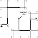
Figure 1: A configuration of chains placed on a Husimi tree with branching parameter $\sigma=1$. Internal monomers are represented as white circles and endpoint monomers are black circles. The statistical weight of this configuration with 3 chains is $z_{i}^{5}\,z_{e}^{6}$.

The density of endpoint monomers is $\rho_{e}=\langle N_{e}\rangle/V$, the density of internal monomers is $\rho_{i}=\langle N_{i}\rangle/V$, and the total density of monomers is $\rho=\rho_{e}+\rho_{i}$. The densities may be obtained from the partition function as follows:

$$\rho_{i}=\frac{z_{i}}{V\Xi}\frac{\partial{\Xi}}{\partial z_{i}},$$ (3)

and

$$\rho_{e}=\frac{z_{e}}{V\Xi}\frac{\partial{\Xi}}{\partial z_{e}}.$$ (4)

Let us now consider the model defined on a Husimi tree (or cactus), which is a Cayley tree built with squares. The branching parameter will be equal to $\sigma$, so that the coordination number of the tree is $q=2(\sigma+1)$. In Fig. 1 a tree with three generations of squares is shown. The tree has a hierarchical structure which allows many statistical mechanical models to be solved in quite simple ways, similar to the ones used on Cayley trees and Bethe lattices b82 . To solve the model on a Husimi tree, it is convenient to consider rooted subtrees, with a square at the root connected to $3\sigma$ other subtrees with one generation less. The configuration of the two bonds incident on the root site of the subtrees is fixed, and we define partial partition functions (ppf’s) on these subtrees for fixed root configurations. The possible root configurations are depicted in Fig. 2, so that partial partition function $g_{0}$ corresponds to a root configuration without any bond coming from above, $g_{i},i=1,2,3,\ldots$ are related to root configurations with a single bond coming from above, connected to $i$ monomers. Finally, the partial partition function $h$ corresponds to a root configuration with two incoming bonds. The root configurations with one incoming bond have been split into the cases where the bond is already attached to $i$ monomers since we later will be interested in obtaining the distribution of sizes of the chains. It will be useful to define the sum of all partial partition functions with a single incoming bond:

$$k=\sum_{i=1}^{\infty}g_{i}.$$ (5)

Figure 2: The root configurations of the subtrees

Now we obtain expressions for the partial partition functions of subtrees with $n+1$ generations of squares in term of the ones of subtrees with $n$ generations of squares. This may be done considering the operation of attaching 3 groups of $\sigma$ smaller subtrees to a new root square. As an example, the recursion relation for a subtree without any bond incident on the root site will be:

$$g_{o}^{\prime} = (g_{0}^{\sigma}+\sigma z_{e}g_{0}^{\sigma-1}k+\frac{\sigma(\sigma-1)}{2}z_{i}g_{0}^{\sigma-2}k^{2}+\sigma z_{i}h)^{3}+$$ (6)

$$(z_{e}g_{0}^{\sigma}+\sigma z_{i}kg_{0}^{\sigma-1})^{2}\,[2(g_{0}^{\sigma}+\sigma z_{e}g_{0}^{\sigma-1}k+$$

$$\frac{\sigma(\sigma-1)}{2}z_{i}g_{0}^{\sigma-2}k^{2}+\sigma z_{i}h)+z_{i}g_{0}^{\sigma}].$$

The first term in the sum corresponds to a configuration of the root square without any polymer bond on its edges. Similar recursion relations may be obtained for the other ppf’s, but since they are rather long they will not be written down here. When these recursion relations are iterated, we obtain the ppf’s of a subtree with additional generations of sites. As expected, these partition functions diverge in the thermodynamic limit.

Let us now define the ratios of partial partition functions:

$$G_{i} = \frac{g_{i}}{g_{0}},\;i=1,2,\ldots$$ (7a)

$$H = \frac{h}{g_{0}},$$ (7b)

$$K = \frac{k}{g_{0}}=\sum_{i=1}^{\infty}G_{i}.$$ (7c)

As seen in the explicit recursion relation presented above, some linear combinations of partial partition functions appear repeatedly, so it is convenient to define them here:

$$a = g_{0}^{\sigma}A=g_{0}^{\sigma}\left[1+\sigma z_{e}K+\frac{\sigma(\sigma-1)}{2}z_{i}K^{2}\right.$$ (8)

$$\left.+\sigma z_{i}H\right],$$

$$b = g_{0}^{\sigma}B=g_{0}^{\sigma}(z_{e}+\sigma z_{i}K),$$ (9)

The recursion relations for the ratios of partial partition functions are:

$$G_{1}^{\prime} = \frac{2z_{e}(A^{2}+B^{2})}{D},$$ (10a)

$$G_{2}^{\prime} = \frac{2z_{i}[\sigma(A^{2}+B^{2})G_{1}+z_{e}A]}{D},$$ (10b)

$$G_{3}^{\prime} = \frac{2z_{i}[\sigma(A^{2}+B^{2})G_{2}+\sigma z_{i}AG_{1}+z_{i}z_{e}]}{D},$$ (10c)

$$G_{i}^{\prime} = \frac{2\sigma z_{i}[(A^{2}+B^{2})G_{i-1}+z_{i}AG_{i-2}+z_{i}^{2}G_{i-3}]}{D}$$ (10d)

$$(i\geq 4),$$

$$H^{\prime} = \frac{(A+2z_{i})B^{2}}{D},$$ (10e)

where $D=A^{3}+B^{2}(2A+z_{i})$. Summing the recursion relations for the $G_{i}$ leads to:

$$K^{\prime} = \sum_{i=1}^{\infty}G_{i}^{\prime}$$ (11)

$$= \frac{2B(A^{2}+B^{2}+z_{i}A+z_{i}^{2})}{D}.$$

In the thermodynamic limit, the behavior of the model will be described by the fixed point values of the infinite set of recursion relations Eqs. (10). The linearity of these recursion relations with respect to the ratios $G_{i}$ allows us to assure that a fixed point of the pair of recursion relations Eqs. (10e) and (11), $H^{\prime}=H,K^{\prime}=K$, is also a fixed point of the whole set of recursion relations pair of recursion relations, so that we restrict ourselves to this reduced set of equations. Due to the non-linearity of these equations, we were not able to find closed expressions of the fixed point values $H(z_{i},z_{e};\sigma)$ and $K(z_{i},z_{e};\sigma)$ in general, but their numerical determination is straightforward. Two particular cases where the fixed point equations simplify are when only dimers are allowed ($z_{i}=0$) and the polymer limit ($z_{e}\to 0$). In these limits the recursion relations above reduce to results in the literature so90 . Once the fixed point values of $K$ and $H$ are found, it is easy to determine the remaining ratios $G_{1},G_{2},\ldots$ using the equations above. The partition function of the model on the Husimi tree may then be obtained considering the operation of attaching $\sigma+1$ subtrees to the central site:

$$\Xi=g_{0}^{\sigma+1}\left[1+(\sigma+1)\left(z_{e}K+z_{i}H+\frac{\sigma}{2}z_{i}K^{2}\right)\right].$$ (12)

We are not interested in the solution of the model on the whole Husimi tree, which is expected to show a behavior which is quite different from the one on regular lattices, and thus concentrate our attention on the behavior at the core of the tree (Husimi lattice). Thus, we obtain the densities of external and internal monomers at the central site, which are easily found considering the contributions to the partition function in Eq. (12) above. The results are:

$$\rho_{e}=\frac{z_{e}K}{\frac{1}{\sigma+1}+z_{e}K+z_{i}H+\frac{\sigma}{2}z_{i}K^{2}},$$ (13)

and

$$\rho_{i}=\frac{z_{i}H+\frac{\sigma}{2}z_{i}K^{2}}{\frac{1}{\sigma+1}+z_{e}K+z_{i}H+\frac{\sigma}{2}z_{i}K^{2}}.$$ (14)

.

The entropy per site $s(\rho_{e},\rho_{i})$ is related to the activities through the equations of state:

$$\ln z_{e}=-\left(\frac{\partial s}{\partial\rho_{e}}\right)_{\rho_{i}},$$ (15)

and

$$\ln z_{i}=-\left(\frac{\partial s}{\partial\rho_{i}}\right)_{\rho_{e}}.$$ (16)

The entropy may then be obtained inverting Eqs. (13) and (14) to obtain $z_{e}(\rho_{e},\rho_{i})$ and $z_{i}(\rho_{e},\rho_{i})$ and then performing the integration:

$$s(\rho_{e},\rho_{i})=-\int_{0}^{\rho_{e}}\ln z_{e}(\rho,0)d\rho-\int_{0}^{\rho_{i}}\ln z_{i}(\rho_{e},\rho)d\rho.$$ (17)

The first integral may be performed analytically, since in the dimer limit the fixed point equations are exactly solvable. The resulting expression is so90 :

$$s(\rho_{e},0) = -(1-\rho_{e})\ln(1-\rho_{e})-\frac{\rho_{e}}{2}\ln\frac{\rho_{e}}{q}+$$ (18)

$$+\frac{1}{2}\left(\frac{q}{2}-\rho_{e}\right)\ln\left(1-\frac{2\rho_{e}}{q}\right)+$$

$$\frac{1}{2}\left(\frac{q}{2}-\rho_{e}\right)\ln(1+W)-$$

$$-\frac{q}{8}\ln(1+2W-W^{2}),$$

where

$$W=\left(1-\frac{q}{2\rho_{e}}\right)+\left[\left(\frac{q}{2\rho_{e}}-1\right)^{2}+1\right]^{1/2}$$ (19)

and $q=2(\sigma+1)$ is the coordination number of the lattice. Now the entropy may be found performing the second integration in Eq. (17) numerically.

We will, however, proceed along a different path, which leads to the same results but with a simpler numerical calculation. We start with an argument proposed by Gujrati g95 to obtain the bulk grand-canonical free energy per site $\phi_{b}$, adapting it to a Husimi lattice built with squares sg05 . This result may be obtained assuming the free energy per elementary square to be a function of the generation of the plaquette in the tree and that in the bulk it will converge to a fixed value in the thermodynamic limit osb10 . A simple derivation for the present case, where we suppose that the center of the Husimi tree is a site, starts by associating a generation number $m$ to each site of the tree, such that $m=0$ for the central site, $m=1$ for the $3(\sigma+1)$ first neighbors of the central site and so on, until the surface of the tree is reached for $m=M$. The number of sites at the surface of the tree will be equal to:

$$N_{s}(M)=3(\sigma+1)(3\sigma)^{M-1}.$$ (20)

The number of remaining sites in the tree, which are in the bulk, will be:

$$N_{b}(M)=1+3(\sigma+1)\sum_{j=0}^{M-2}(3\sigma)^{j}=1+3(\sigma+1)\frac{(3\sigma)^{M-1}-1}{3\sigma-1}.$$ (21)

Supposing that the free energy of the whole tree may be written as a sum of the contributions of its surface and the bulk, we have: $\Phi(M)=-k_{B}T\ln\Xi(M)=N_{b}(M)\phi_{b}+N_{s}(M)\phi_{s}$, where $\phi_{b}$ and $\phi_{s}$ are the free bulk and surface free energies per site, respectively. In the thermodynamic limit $M\to\infty$, we may then find that:

$$-\ln\Xi(M+1)+3\sigma\ln\Xi(M)=[N_{b}(M+1)-3\sigma N_{b}(M)]\varphi_{b}$$ (22)

where $\varphi_{b}=\phi_{b}/(k_{B}T)$. The substitution of the expressions (20) and (21) for the numbers of bulk and surface sites we will find that:

$$\varphi_{b}=-\frac{1}{4}\ln\left(\frac{\Xi(M+1)}{\Xi(M)^{3\sigma}}\right).$$ (23)

This expression is a generalization of the one obtained using a similar argument by Semerianov and Gujrati for $\sigma=1$ (expression A7 in sg05 ). If we now substitute the partition function (12) in the expression above and observe that $g_{0}(M+1)/(g_{0})^{3\sigma}$ is equal to the fixed point value of the denominator of the recursion relations (10e) $D$, so that

$$\varphi_{b}=$$

$$-\frac{1}{4}\ln\left[\frac{D^{\sigma+1}}{[1+(\sigma+1)(z_{e}K+z_{i}H+\sigma z_{i}K^{2}/2)]^{3\sigma-1}}\right],$$ (24)

where the thermodynamic limit is implicit since the fixed point values of $D$, $K$, and $H$ are used.

The entropy per site in the bulk of the tree is given by the state equation:

$$s=-\left(\frac{\partial\phi_{b}}{\partial T}\right)_{\mu_{e},\mu_{i}},$$ (25)

which leads to the expression:

$$\frac{s}{k_{B}}=-\varphi_{b}-\rho_{e}\ln z_{e}-\rho_{i}\ln z_{i}.$$ (26)

Solving equations (13) and (14) for the activities $z_{e}$ and $z_{i}$, we obtain the equations:

$$\rho_{e}=z_{e}K(\sigma+1)(1-\rho_{e}-\rho_{i}),$$ (27)

and

$$\rho_{i}=z_{i}(\sigma+1)(H+\sigma K^{2}/2)(1-\rho_{e}-\rho_{i}).$$ (28)

To obtain the entropy as a function of the densities of internal monomers and endpoint monomers, we numerically solve the set of four equations (27), (28), (10e), and (11) (making $H^{\prime}=H$ and $K^{\prime}=K$ in the last two equations), so that we obtain $z_{e}$, $z_{i}$, $H$, and $K$ as functions of the densities, and then the entropy per site in the bulk using expression (26). In general, this numerical procedure converges to the fixed point and leads to accurate results, but there are problems when the full lattice limit is approached, as expected, since the activities diverge in this limit. Therefore, to compute the entropy in the full lattice limit we use a separate procedure we will describe below. We thus take the limit of diverging fugacities keeping $z=z_{e}/z_{i}=\exp[(\mu_{e}-\mu_{i})/(k_{B}T)]$ fixed. In this limit, the variables defined in expressions (8) and (9) diverge and it is convenient to define the new variables

$$A_{\infty} = \frac{A}{z_{i}}=\sigma zK+\frac{\sigma(\sigma-1)}{2}K^{2}+\sigma H,$$ (29a)

$$B_{\infty} = \frac{B}{z_{i}}=z+\sigma K,$$ (29b)

$$D_{\infty} = =\frac{D}{z_{i}^{3}}=A_{\infty}^{3}+B_{\infty}^{3}(2A_{\infty}+1),$$ (29c)

and the recursion relations may be rewritten as

$$H^{\prime} = \frac{B_{\infty}^{2}(A_{\infty}+2)}{D_{\infty}},$$ (30)

$$K^{\prime} = \frac{2B_{\infty}(A_{\infty}^{2}+B_{\infty}^{2}+A_{\infty}+1)}{D_{\infty}}.$$ (31)

The density of endpoint monomers will be given by:

$$\rho_{e}=\frac{zK}{zK+H+\sigma K^{2}/2},$$ (32)

and we notice that in the limit $z\to\infty$, which corresponds to the lattice fully covered with dimers, we find that $\rho_{e}\to 1$, while for $z\to 0$ we have $\rho_{e}\to 0$, as expected. The density of internal monomers will be $\rho_{i}=1-\rho_{e}$, and the mean number of monomers per chain is ${\bar{M}}=2/\rho_{e}$. Substitution of equation (32) in this last expression leads to:

$$H=\frac{K}{2}[z({\bar{M}}-2)-\sigma K].$$ (33)

This last expression allows us to eliminate $H$ from the fixed point equations associated to the recursion relations (10e) and (11), so that the fixed point equations reduce to:

$$\frac{K}{2}[z({\bar{M}}-2)-\sigma K]D_{\infty}=(A_{\infty}+2)B_{\infty}^{2},$$ (34)

$$KD_{\infty}=2B_{\infty}[A_{\infty}(1+A_{\infty})+B_{\infty}+1].$$ (35)

For fixed values of the mean molecular weight of the chains ${\bar{M}}$, these equations may numerically be solved for $K$ and $z$, using also the equations (29). Once the fixed point is found, we may obtain the entropy noticing that expression (26) in the full lattice limit reduces to $s/k_{B}=-\varphi_{b}-\rho_{e}\ln z-\ln z_{i}$, and substitution of the bulk free energy in this limit allows us to write the entropy as:

$$\frac{s}{k_{B}}=\frac{1}{4}\ln\frac{D_{\infty}^{\sigma+1}}{[(\sigma+1){\bar{M}}zK/2]^{3\sigma-1}}-\frac{2}{{\bar{M}}}\ln z.$$ (36)

Figure 3: Entropy as a function of the density of monomers $\rho=\rho_{e}+\rho_{i}$ for polydisperse chains on the Husimi lattice. In the region of small densities, the curves shown correspond to mean molecular weights ${\bar{M}}=3,6,$ and $10$ in downward order. The results are for $\sigma=1$ ($q=4$).

Figure 4: Entropy as a function of the mean molecular weight at full coverage for a Husimi lattice with $\sigma=1$ ($q=4$).

On the Bethe lattice, it is possible to obtain an the entropy explicitly using the expression for the bulk free energy, and we show this calculation in some detail in the Appendix.

Results for the entropy as a function of the total density of sites, for fixed values of the mean molecular weight ${\bar{M}}=2(\rho_{e}+\rho_{i})/\rho_{e}$ are displayed in figure 3. As was already noticed in the results on the Bethe lattice, the entropy is a increasing function for small values of the density and goes through a maximum at intermediate densities. We notice that at low densities the entropy is a decreasing function of the mean molecular weight ${\bar{M}}$, but this does not hold for larger densities.

Figure 5: Relative differences between the entropies of polydisperse chains on Bethe ($s_{B}$) and Husimi ($s_{H}$) lattices as functions of the density for lattices with $q=4$. From the upper to the lower curve, the mean molecular weights are equal to 10, 6, and 3.

Figure 6: Relative differences between the entropies of polydisperse chains on Bethe ($s_{B}$) and Husimi ($s_{H}$) lattices as functions of the density for ${\bar{M}}=6$. From the upper to the lower curve, the coordination numbers are equal to 4, 6, 8, 10, and 12. Numerical round-off errors are already visible at higher coordination numbers, particularly at low densities.

It is interesting to compare the present results with the ones for the Bethe lattice ns08 . In general, as was also found in the monodisperse case so90 , both results are quite close. In figure 5 the relative differences between both entropies are given as functions of the density for some values of ${\bar{M}}$, in general these differences are in a range below 1%. At low densities, the entropy on the Bethe lattice is larger than the one on the Husimi lattice, but the opposite may happen at higher densities. The difference between the results on both lattices reduces as the coordination number $q$ is increased, as expected, since in the limit $q\to\infty$ both entropies are equal to the simple mean field estimate, this is apparent in the plots displayed in figure 6.

$M$	Bethe (m)	Husimi (m)	Bethe (p)	Husimi (p)
$2$	$\ \ 0,26162$	$\ \ 0,26743$	$\ \ 0,26162$	$\ \ 0,26743$
$3$	$\ \ 0,42284$	$\ \ 0,41295$	$\ \ 0,88493$	$\ \ 0,88650$
$4$	$\ \ 0,48166$	$\ \ 0,48951$	$\ \ 0,95904$	$\ \ 0,95969$
$5$	$\ \ 0,50669$	$\ \ 0,50888$	$\ \ 0,95656$	$\ \ 0,95673$
$6$	$\ \ 0,51349$	$\ \ 0,51265$	$\ \ 0,93473$	$\ \ 0,93467$
$7$	$\ \ 0,52217$	$\ \ 0,52284$	$\ \ 0,90836$	$\ \ 0,90820$
$\infty$	$\ \ 0,4055$	$\ \ 0,4090$	$\ \ 0,4055$	$\ \ 0,4090$

Table 1: Entropy at full coverage for lattices with $q=4$. Results for monodisperse (m) and polydisperse (p) chains are shown. Data for the monodisperse case are from reference so90 and the case of polydisperse chains on the Bethe lattice is discussed in ns08 .

In the table 1 we present data for the entropy at full coverage ($\rho=1$). As mentioned before for the general case, the differences, both in the monodisperse and the polydisperse systems, between the results of the Bethe lattice and of the Husimi lattice solutions are quite small, and there are indications that these values are still rather far away from the results for regular lattices with the same coordination number. For dimers ($M=2$), where there is no polydispersity in our model, the exact value on the square lattice is known fkt61 ($s_{2}=G/\pi\approx 0.29156$, $G$ is Catalan’s constant). In this case, the value on the Bethe lattice is about 10% below the exact value, while on the Husimi lattice the difference reduces to roughly 8%. The entropy for monodisperse chains with $M>2$ calculated on Bethe and Husimi lattices is always larger than the estimates obtained from transfer matrix calculations for the square lattice ds03 , and the relative differences are smaller than the ones for dimers. In the polymer limit $M\to\infty$, the difference between the entropies for the poly- and monodisperse cases vanishes again.

We notice that the entropy at full coverage is not a monotonic function of the mean molecular weight, showing a maximum around ${\bar{M}}\approx 4.37$, as may be seen in figure 4. As expected, on the Husimi lattice we find that the entropy for polydisperse chains is always larger or equal to the one for monodisperse chains with $M$ monomers for the same density of monomers $\rho$ and finite ${\bar{M}}=M>2$, obtained in so90 , where equality holds only for vanishing density.

On the Bethe lattice, it was possible to obtain the entropy for polydisperse chains analytically, and it was found that the contribution of polydispersity to the entropy,

$$\Delta s_{M}(\rho)=s_{\bar{M}}(\rho)-s_{M}(\rho),$$ (37)

with $M=\bar{M}$, is linear in $\rho$ and independent of $q$ ns08 : $\Delta s_{M,B}=\rho[(M-1)\ln(M-1)-(M-2)\ln(M-2)]/M$. The contribution to the entropy of polydispersity in the solution of the model on the Husimi lattice ($\Delta s_{M,B}$ does not show such a simple behavior. In figure 7 we show the difference between the results on the Bethe and on the Husimi lattices, for different values of the molecular weight $M$. We notice that in general, as the molecular weight $M$ is increased, the Husimi lattice results are closer to the ones found on the Bethe lattice. This may be understood if we remember that since no loops are present on the Bethe lattice and loops of four edges only may be found on the Husimi lattice we considered, a reasonable effect of these closed paths should be expected for chains of length close to four, but these effects should become smaller as the chains grow. In opposition to what is found on the Bethe lattice, the contribution of polydispersity to the entropy on the Husimi lattice solution changes as the branching parameter $\sigma$ varies. This may be seen in figure 8. In general, we find that the Husimi lattice results become closer to the ones found on the Bethe lattice as $\sigma$, and therefore the coordination number $q$, grow. This is expected, since both solutions should become equal to the simple mean field solution in the limit $q\to\infty$. However, as is apparent in the curves in figure 8, the convergence is not monotonic.

Figure 7: Difference between the contribution of polydispersity on the Bethe and the Husimi lattice solutions as a function of the density $\rho$. The full curve is for $M=\bar{M}=3$, the dashed one for $M=\bar{M}=4$ and the dotted one for $M=\bar{M}=5$. All results are for $\sigma=1$ ($q=4$).

Figure 8: Difference between the contribution of polydispersity on the Bethe and the Husimi lattice solutions as a function of the density $\rho$. The full curve is for $\sigma=1$, the dashed one for $\sigma=2$ and the dotted one for $\sigma=3$ ($q=6,4,8$, respectively). All curves are for $M=\bar{M}=4$.

To calculate the probability $r_{M}$ to find a chain with $M$ monomers among all chains, we notice that:

$$r_{M}=\frac{G_{M-1}}{K},$$ (38)

and this probability can be numerically evaluated, since we may obtain the functions $G$ and $K$, whose recursion relations are given in Eqs. (10e) and (11), at the fixed point. We recall that on the Bethe lattice these ratios are given by $B_{B}=r_{M+1}/r_{M}=({\bar{M}}-2)/({\bar{M}}-1)$, and therefore are independent of $\rho$ and $q$ ns08 . As may be noted in Fig. 9, where the ratios $B_{H}(M)=r_{M+1}/r_{M}$ are plotted as functions of $M$, for small values of $M$ compared to 4 the distribution of molecular weights is not exponential, but as $M\gg 4$ an exponential behavior is apparent. The value 4 corresponds to the size of the only possible closed path on the lattice we considered. Again, we notice that the deviations from the exponential behavior are larger for smaller values of $q$, as $q$ increases the results approach an exponential behavior for all values of $M$, as found on the Bethe lattice. The asymptotic value of the ratio for large values of $M$ may be found by assuming an exponential decay of the probabilities for the fixed point values of the ratios of partial partition functions $G_{i}$ for $i>3$ in Eqs. (10e), which leads to the following equation for the limiting ratio $B_{H}=\lim_{M\to\infty}r_{M+1}/r_{M}$:

$$B_{H}^{3}-\frac{2\sigma z_{i}}{D}[(A^{2}+B)\,B_{H}^{2}+z_{i}A\,B_{H}+z_{i}^{2}]=0,$$ (39)

and the horizontal line in Fig. 9 was obtained solving this equation.

Figure 9: Ratios of probabilities to find chains with successive molecular weights $M$ on the Husimi lattice $B_{H}(M)$ as functions of the molecular weight $M$ for ${\bar{M}}=3$. Data shown are for $\sigma=1$ and $\rho=0.3019045$. The dashed line corresponds to the result on the Bethe lattice, which for this case is $B_{B}=1/2$. The full line is the asymptotic value $B_{H}=\lim_{M\to\infty}B_{H}(M)$.

The asymptotic ratio of the solution on the Husimi lattice, $B_{H}$, in general will be a function of $\bar{M}$, $\sigma$ and $\rho$. In figure 10 this is apparent, and again we notice that as the coordination number of the lattice become larger, the result on the Husimi lattice approaches the one found on the Bethe lattice. This may be seen analytically in the limit of vanishing activities. Expanding the recursion relations up to the lowest nonzero order of $z_{e}$ and $z_{i}$, we get:

$$H^{\prime} = z_{e}^{2}+2\sigma z_{e}z_{i}K+(\sigma z_{i}K)^{2},$$ (40a)

$$K^{\prime} = 2z_{e}+2\sigma z_{i}K.$$ (40b)

It is then easy to find the fixed point values up to lowest non-vanishing order $K^{*}=2z_{e}$ and $H^{*}=z_{e}^{2}$, and the corresponding values for the mean molecular weight $\bar{M}=2+(1+2\sigma)z_{i}$ and density of monomers $\rho=2(\sigma+1)z_{e}^{2}$. The approximate solution of the equation (39) for the decay exponent in the limit of small activities is $\beta_{H}=2\sigma z_{i}$, which may be combined with the expression for $\bar{M}$ above leading to:

$$\beta_{H}=\frac{2\sigma}{1+2\sigma}(\bar{M}-2),$$ (41)

where the dependence of the exponent with $\sigma$ in the limit considered is clear. In general, the exponent will also be a function of $\rho$, but, as may be seen above, in the limit we consider here this contribution is of higher order. The same expansion may be done for the Bethe lattice solution ns08 , and leads to the result $\beta_{B}=\sigma^{\prime}z_{i}$, where $\sigma^{\prime}$ is the branching parameter of this lattice. If we compare Bethe and Husimi lattices with the same coordination numbers, we have $\sigma^{\prime}=2\sigma+1$, and as expected $\beta_{H}\to\beta_{B}$ as $\sigma\to\infty$.

Figure 10: Asymptotic coefficient $B_{H}$ as a function of the density $\rho$, calculated for ${\bar{M}}=6$. The lowest curve corresponds to $\sigma=1$ $(q=4)$ and the following ones in upward order to $\sigma=2,\;3$ $(q=6,\;8)$. The dashed line corresponds to coefficient for the Bethe lattice $B_{B}=4/5$.

III Final comments and discussions

We have studied an athermal model of flexible chains with excluded volume interactions only on a Husimi lattice built with squares, with an arbitrary value for the branching parameter $\sigma$, so that the coordination number of the lattice is $q=2(\sigma+1)$. The chains are linear and composed by a set of monomers, so that consecutive monomers occupy first neighbor sites of the lattice. They are polydisperse, and the distribution of sizes is determined in an annealed way by two parameters: the activity $z_{e}$ of an endpoint monomer (linked to one other monomer of the chain only) and $z_{i}$ of an internal monomer, which is linked to two other monomer of its chain.

The entropy as a function of the fraction of sites occupied by monomers and the mean number of monomers in each chain (mean molecular weight of the chains) is a fundamental equation of the system in the thermodynamic sense, and we have obtained this function in general on the Husimi lattice, although, at variance to what was done in the solution of this problem on the Bethe lattice ns08 , we were not able to derive a closed form for it. We found that the differences between results on Bethe and Husimi lattices with the same coordination numbers s rather small, below 1%, as was also the case for monodisperse chains so90 . It is also possible that the results on the Husimi lattice for $q=4$ are still not very close to the ones on the square lattice, although, to our knowledge, no results for the entropy of this model on regular lattices are available in the literature. For the monodisperse rather precise estimates were obtained using the transfer matrix approach ds03 , and we are presently extending these results for the polydisperse model on the square lattice. It is expected that the results on the Husimi lattice will be closer to the ones on regular lattices at higher dimensions, but again there are no estimates of the entropy of the model available in the literature for three-dimensional lattices, for example.

Another point which should be further investigated is the distribution of molecular weights of the chains. The simple exponential distribution which was found on the Bethe lattice ns08 is no longer valid on the Husimi lattice, so we expect that on regular lattices a different size distribution will be found too. It may be that this question could be addressed on the square lattice with transfer matrix techniques, we are now investigating this possibility.

Appendix A Free energy of the model on Bethe lattice

On a Bethe lattice with arbitrary coordination number $q$, the entropy of chains whose polydispersity is determined by different activities for internal and endpoint monomers may be calculated exactly. Here we show that this result, which was originally obtained integrating the expressions for monomer densities, may also be found more directly by derivation of the bulk free energy calculated using Gujrati’s prescription. Recalling the discussion of the problem in ns08 , we define a partial partition functions $g_{0}$ and $g_{1}$ for subtrees with and without a polymer bond on the root edge, respectively. The recursion relation for the ratio $R=g_{1}/g_{0}$ of these ppf’s is given by expression (13) in this paper:

$$R^{\prime}=\frac{z_{e}+\sigma z_{i}R}{1+\sigma z_{e}R+\frac{\sigma(\sigma-1)}{2}z_{i}R^{2}},$$ (42)

and equation (14) for the partition function of the model on the Cayley tree may be written as:

$$\Xi = g_{0}^{q}+qz_{e}g_{0}^{q-1}g_{1}+\frac{q(q-1)}{2}z_{i}g_{0}^{q-2}g_{1}^{2}$$ (43)

$$= g_{0}^{q}\left[1+qz_{e}R+\frac{q(q-1)}{2}z_{i}R^{2}\right].$$

The free energy of the model on the Bethe lattice corresponds to free energy on the bulk of the Cayley tree, and denoting this free energy per site of the tree by $\phi_{b}$ we obtain, using Gujrati’s ansatz, the result oss09 :

$$\varphi_{b}=\frac{\phi_{b}}{k_{b}T}=-\frac{1}{2}\ln\frac{\Xi_{m+1}}{\Xi_{m}^{q-1}},$$ (44)

where $m$ denotes the number of generations in the tree and we are interested in the thermodynamic limit $m\to\infty$. Using expression (43) for the partition function, we get:

$$\varphi_{b}=-\frac{1}{2}\ln\left\{\left(\frac{g_{0}^{\prime}}{g_{0}^{q-1}}\right)^{q}\frac{1}{\left[1+qz_{e}R+\frac{q(q-1)}{2}z_{i}R^{2}\right]^{q-2}}\right\},$$ (45)

and recalling the recursion relation for $g_{0}$ (expression (11)), which is:

$$g_{0}^{\prime}=g_{0}^{\sigma}+\sigma z_{e}g_{0}^{\sigma-1}g_{1}+\frac{\sigma(\sigma-1)}{2}z_{i}g_{0}^{\sigma-2}g_{1}^{2},$$ (46)

we reach the following expression for the bulk free energy per site:

$$\varphi_{b}=-\frac{1}{2}\ln\left[\frac{\left(1+\sigma z_{e}R+\frac{\sigma(\sigma-1)}{2}z_{i}R^{2}\right)^{q}}{\left(1+qz_{e}R+\frac{q(q-1)}{2}z_{i}R^{2}\right)^{q-2}}\right].$$ (47)

Now the entropy is given as a state equation associated to the free energy, whose expression is equation (26) above. since the activities may be written as functions of the densities in the core of the tree, expression (25) in ns08 for the entropy as a function of these densities is found.

References

- (1) R. H. Fowler and G. S. Rushbrooke, Trans. Faraday Soc. 33, 1272 (1937).
- (2) M. E. Fisher, Phys. Rev. 124, 1664 (1961); P. W. Kasteleyn, Physica 27, 1209 (1961); H. N. V. Temperley and M. E. Fisher, Philos. Mag. 6, 1061 (1961).
- (3) F.Y. Wu, Phys. Rev. E 74 020140(R) (2006); Erratum, Phys. Rev. E 74 020104(E) (2006).
- (4) J. F. Nagle, C. S. O. Yokoi, and S. M. Battacharjee, Phase Transitions and Critical Phenomena, volume 13, edited by C. Domb and J. L. Lebowitz Academic, London, (1989).
- (5) S. R. Salinas and J. F. Nagle, Phys. Rev. B 9, 4920(1974).
- (6) A. M. Nemirovsky and M. D. Coutinho-Filho, Phys. Rev. A 39, 3120 (1989).
- (7) J. F. Stilck and M. J. de Oliveira, Phys. Rev. A 42, 5955 (1990).
- (8) W. G. Dantas and J. F. Stilck, Phys. Rev. E 67, 031803 (2003); W. G. Dantas, M. J. de Oliveira and J. F. Stilck, Phys. Rev. E 76, 031133 (2007).
- (9) J. C. Wheeler, S. J. Kennedy and P. Pfeuty, Phys. Rev. Lett. 45, 1748 (1980); J. C. Wheeler and P. Pfeuty, Phys. Rev. A 24, 1050 (1981); P. D. Gujrati, Phys. Rev. B 24, 2854 (1981) and Phys. Rev. A 24, 2096 (1981).
- (10) P. D. Gujrati, S. S. Rane, and A. Corsi, Phys. Rev. E 67, 052501 (2003); A. Corsi and P. D. Gujrati, Phys. Rev. E 68, 031502 (2003).
- (11) P. D. Gujrati, J. Phys. A: Math. Gen. 34, 9211 (2001).
- (12) R. Baxter, Exactly solved models in statistical mechanics, (1982).
- (13) P. D. Gujrati, Phys. Rev. Lett. 74, 809 (1995).
- (14) J. F. Stilck and J. C. Wheeler, J. Stat. Phys. 46, 1 (1987).
- (15) M. A. Neto and J. F. Stilck, J. Chem. Phys. 128, 184904 (2008), see also P. D. Gujrati, J. Chem. Phys. 130, 057101 (2009).
- (16) J. F. Stilck, M. A. Neto, and W. G. Dantas, Physica A 368, 442 (2006).
- (17) L. Schäfer, Phys. Rev. B 46, 6061 (1992).
- (18) F. Semerianov and P. Gujrati, Phys. Rev. E 72, 011102 (2005).
- (19) T. J. Oliveira,J. F. Stilck, and M. A. A. Barbosa, Phys. Rev. E 82, 051131 (2010).
- (20) T. J. Oliveira, J. F. Stilck, and P. Serra, Phys. Rev. E 80, 041804 (2009).