Generating Very-High-Precision Frobenius Series
with Apriori Estimates of Coefficients

Abstract

The Frobenius method can be used to compute solutions of ordinary linear differential equations by generalized power series. Each series converges in a circle which at least extends to the nearest singular point; hence exponentially fast inside the circle. This makes this method well suited for very-high-precision solutions of such equations. It is useful for this purpose to have prior knowledge of the behaviour of the series. We show that the magnitude of its coefficients can be apriori predicted to surprisingly high accuracy, employing a Legendre transformation of the WKB approximated solutions of the equation.

Second order ODEs, Regular singular points, Frobenius method, Legendre transformation, WKB approximation.

1 Introduction

A large set of problems from technology and science involves the study of linear second order ordinary differential equations. Although the original problem is more likely to be a partial differential equation involving the Laplace operator in two or higher dimensions, it is often possible to reduce it to a set of one-dimensional problems through separation of variables.

For example, in three dimensions the wave, heat, or Schrödinger equation in zero or constant potential can be separated in ellipsoidal coordinates $\left(\xi_{1},\xi_{2},\xi_{3}\right)$, related to cartesian coordinates by

$$x =\sqrt{\frac{(\xi_{1}^{2}-a^{2})(\xi_{2}^{2}-a^{2})(\xi_{3}^{2}-a^{2})}{a^{2}(a^{2}-b^{2})}},$$

$$y =\sqrt{\frac{(\xi_{1}^{2}-b^{2})(\xi_{2}^{2}-b^{2})(\xi_{3}^{2}-b^{2})}{b^{2}(b^{2}-a^{2})}},$$ (1)

$$z =\frac{\xi_{1}\xi_{2}\xi_{3}}{ab},$$

where $\xi_{1}>a>\xi_{2}>b>\xi_{3}>0$, plus 10 degenerate forms of these coordinates [1]. The separated equations have five regular singular points, at $\pm a$, $\pm b$, and $\infty$ [2]. This means that the equations can be formulated as second order equations with polynomial coefficients. The majority of the special functions of mathematical physics, as f.i. discussed by Whittaker and Watson [3], can be described as solutions to such equations.

The Schrödinger equation remain separable if we add a potential of the form

$$V=\frac{(\xi_{2}^{2}-\xi_{3}^{2})u(\xi_{1})+(\xi_{1}^{2}-\xi_{3}^{2})v(\xi_{2})+(\xi_{1}^{2}-\xi_{2}^{2})w(\xi_{3})}{(\xi_{1}^{2}-\xi_{2}^{2})(\xi_{1}^{2}-\xi_{3}^{2})(\xi_{2}^{2}-\xi_{3}^{2})}.$$ (2)

The degenerate forms often lead to situations where two or more regular singular points merge to irregular singular points (confluent singularities).

It is sometimes useful to evaluate solutions to much higher accuracy than possible with standard double-precision methods. Recently we have developed and used code for solving a large class of ordinary Frobenius type equations to almost arbitrary high precision, in a number of algebraic operations $N$ which grows asymptotically linearly with the desired precision $P$, i.e.

$$N\approx N_{0}+\text{const}\,P.$$ (3)

It was f.i. used in [4] to find the lowest eigenvalue of

$$-\psi^{\prime\prime}(x)+x^{4}\psi(x)=\varepsilon\psi(x)$$ (4)

to an accuracy of one million decimals digits, and its eigenvalue number $50\,000$ to $50\,000$ decimal digits. It was further demonstrated in [5] that it is possible to compute normalization integrals of the resulting wavefunctions to comparable precision. The method also extends to computation of many other types of amplitudes.

In reference [6] we have published and tested code for solving equations of the class

$$-\!\left(\frac{d^{2}}{dz^{2}}+\frac{1\!-\!\nu_{+}\!-\!\nu_{-}}{z}\frac{d}{dz}+\frac{\nu_{+}\nu_{-}}{z^{2}}\right)\psi(z)+\frac{1}{z}\sum_{n=0}^{N}\text{v}_{n}\,z^{n}\,\psi(z)=0.$$ (5)

I.e., equations with polynomial coefficients (after multiplication by $z^{2}$), and at most one regular singular point in the finite plane.

When implementing the Frobenius method [7] numerically the solution is represented by a convergent series

$$\psi(z)=\sum_{m=0}^{\infty}a_{m}\,z^{m+\nu},$$ (6)

where the coefficients $a_{m}$ is generated recursively in parallel with the accumulation of the sum of the series. The method is straightforward to extend to the wider class of equations (9), but this requires consideration of several special cases.

The individual terms in (6) may grow very big, leading to huge cancellations and large roundoff errors. It is therefore useful to have some prior knowledge of the magnitude of the $a_{m}$’s before a high-precision evaluation — to set the computational precision required for a desired accuracy of the final result, and to estimate the time required to complete the computation. There is also the question whether one should evaluate $\psi(z)$ directly at some far away point $z$, or if it is better to make one or more steps of analytic continuation. I.e., evaluate $\psi(z_{i})$ and $\psi^{\prime}(z_{i})$ at one or more intermediate points $z_{i}$. Analytic continuation of functions which satisfy a second order differential equation is rather simple to implement, since the function is fully specified by just two complex numbers $\psi(z_{i})$ and $\psi^{\prime}(z_{i})$, plus the differential equation.

We have found that $|a_{m}|$ can be estimated surprisingly accurate from a WKB approximation of the solution, followed by a Legendre transform with additional corrections. For the general class of equations (5), or its extension to (9), the WKB integrals and the Legendre transform must be done by numerically, but for this one can employ standard double-precision methods. The rest of this paper is organized as follows:

In section 2 we give a systematic presentation of all explicit formulas for a Frobenius series solutions of equation (9) around ordinary and regular singular points, also considering the special cases where logarithmic terms will or may occur.

In section 3 we first give a brief motivation of the method of Legendre transformations, from the point of view of evaluating partition function integrals of statistical physics. We next show how the method may be improved by a “finite size correction”, and demonstrate how it works on an example with known result. Although the correction method was motivated by our desire to estimate the coefficients of (6) more accurately, it should also be applicable to the statistical mechanics of small systems (i.e., systems which must be considered before the thermodynamic limit).

In section 4 we view the sum (6) as a partition function, and apply the method of the previous section to find a relation between the magnitudes $|a_{m}|$ and $|\psi(z)|$. This can be used to estimate $|a_{m}|$ provided we know $|\psi(z)|$.

In section 5 we discuss how one may use the WKB approximation to find a sufficiently good approximation to $\psi(z)$, thereby completing the set of tools required for our estimates.

In section 6 we demonstrate how the method works on a set of examples where much of the calculations may be performed analytically.

A first account of this work has been presented in [8].

2 The Frobenius method for second order ODEs

The Frobenius method for solving homogeneous linear ordinary differential equations is treated in all books on differential equations. However, it is difficult to find general expressions which are sufficiently explicit for implementation as numerical code, and which also cover all special cases. We present such expressions in this section.

We consider the second order differential operator

$${\cal L}=p(z)\frac{d^{2}}{dz^{2}}+q(z)\frac{d}{dz}+r(z),$$ (7)

where

$$p(z) =\sum_{k\geq 0}p_{k}\,z^{k}=C\,\prod_{n\geq 0}(z-z_{n})$$

$$q(z) =\sum_{k\geq 0}q_{k}\,z^{k},\quad r(z)=\sum_{k\geq 0}r_{k}\,z^{k},$$

are (short) polynomials in $z$. Solutions to the equation

$${\cal L}\,\psi(z)=0$$ (9)

in the vicinity of $z=0$, depending on the behaviour of $p(z)$, can often be found by series expansion. For explicit implementation of solution algorithms we must consider several cases.

2.1 Ordinary points

When $p_{0}\neq 0$ the point $z=0$ is an ordinary point for equation (9). The solution can be expanded in a Taylor series,

$$\psi(z)=\sum_{m\geq 0}a_{m}\,z^{m}.$$ (10)

Insertion into equation (9) gives

$${\cal L}\,\psi(z)=\sum_{m\geq 0}\sum_{k\geq 0}P_{k}(m+2)\,a_{m+2-k}\,z^{m}=0,$$ (11)

with

$$P_{k}(\mu)\equiv(\mu-k)\left[(\mu-1-k)p_{k}+q_{k-1}\right]+r_{k-2}.$$ (12)

Here, and in the following, all coefficients with negative indices should be interpreted as zero,

$$a_{-n}=p_{-n}=q_{-n}=r_{-n}=0,\quad\text{for }n=1,2,\ldots.$$

The requirement that the coefficient of each power $z^{m}$ in (11) must vanish leads to the recursion formula

$$a_{m+2}=-\frac{1}{(m+2)(m+1)\,p_{0}}\,\sum_{k\geq 1}P_{k}(m+2)\,a_{m+2-k}.$$ (13)

The coefficients $a_{0}$ and $a_{1}$ can be chosen freely, or according to the initial conditions.

2.2 Regular singular points

When (a) $p_{0}=0$ with $p_{1}\neq 0$ (and at least one of $q_{0}$ or $r_{0}$ is nonzero), or when (b) $p_{0}=p_{1}=q_{0}=0$ with $p_{2}\neq 0$ (and $r_{0}$ is nonzero), equation (9) has a regular singular point at $z=0$. A series solution can be found by the Frobenius method. I.e., one writes the tentative solution as a generalized power series (6).

One solvability condition is that $\nu$ must satisfy a second order algebraic equation. Hence, counting possible degeneracies, there will be two solutions, $\nu_{1,2}$ (choosing $\text{Re}\,\nu_{1}\leq\text{Re}\,\nu_{2}$). We must further consider the cases (i) $\nu_{1}=\nu_{2}$, (ii) $\nu_{2}=\nu_{1}+\ell$ with $\ell$ a positive integer, and (iii) everything else. To avoid explicit implementation of too many special cases we can instead write

$$\psi(z)=z^{\nu_{2}}\,\tilde{\psi}(z),$$ (14)

and solve the resulting equation for $\tilde{\psi}(z)$. The explicit transformation of the polynomial coefficients is

$$\tilde{p}(z) =z^{-1}\,p(z),$$

$$\tilde{q}(z) =2\nu z^{-2}p(z)+z^{-1}q(z),$$ (15)

$$\tilde{r}(z) =\nu(\nu-1)z^{-3}p(z)+\nu z^{-2}q(z)+z^{-1}r(z),$$

where $\tilde{p}(z)$ and $\tilde{q}(z)$ remain polynomials because $p_{0}=p_{1}=q_{0}=0$, and $\tilde{r}(z)$ is a polynomial when

$$\nu(\nu-1)p_{2}+\nu q_{1}+r_{0}=0.$$ (16)

I.e., when $\nu$ satisfies the indicial equation. The transformed equation corresponds to the case (a) above, with index $\tilde{\nu}_{2}=0$ and $q_{0}/p_{1}\geq 1$. The latter implies $\tilde{\nu}_{1}\leq 0$. Henceforth we will only consider this case, dropping $\tilde{\ }$ from the notation. For the computations below we need various cases of the formula (using $P_{0}(\mu)=0$ when $p_{0}=0$),

$${\cal L}\,\sum_{m\geq 0}\left(a_{0,m}+a_{1,m}\log z\right)z^{m+\nu}=$$

$$\sum_{m\geq-1}\Big{\{}\sum_{k\geq 0}\Big{[}P_{k\!+\!1}(m\!+\!2\!+\!\nu)\left(a_{0,m\!+\!1\!-\!k}+a_{1,m\!+\!1\!-\!k}\log z\right)$$

$$+Q_{k\!+\!1}(m\!+\!2\!+\!\nu)\,a_{1,m\!+\!1\!-\!k}\Big{]}\Big{\}}z^{m+\nu},$$ (17)

with $P_{k}(\mu)$ given by equation (12), and

$$Q_{k}(\mu)=(2\mu-1-2k)p_{k}+q_{k-1}.$$ (18)

2.3 Regular singular point with non-integer index difference

First consider the everything else case. We assume a solution of the form (6). Now ${\cal L}\psi(z)=0$ implies

$$\sum_{k\geq 0}P_{k+1}(m+2+\nu)\,a_{m+1-k}=0,$$ (19)

for $m=-1,0,\ldots$. For $m=-1$ this becomes

$$P_{1}(1+\nu)=\nu\left[(\nu-1)p_{1}+q_{0}\right]=0,$$ (20)

with solutions and $\nu_{1}=1-q_{0}/p_{1}$, and $\nu_{2}=0$. In this case $\nu_{1}$ is non-integer. For $m\geq 0$, and $\nu=\nu_{1}$ and $\nu=\nu_{2}=0$ respectively, equation (19) implies the recursion relations

$$a_{m\!+\!1} =\frac{-1}{(m\!+\!1)(m\!+\!1\!+\!\nu_{1})p_{1}}\sum_{k\geq 1}P_{k+1}(m\!+\!2\!+\!\nu_{1})\,a_{m\!+\!1\!-\!k},$$

$$a_{m\!+\!1} =\frac{-1}{(m\!+\!1)(m\!+\!1\!-\!\nu_{1})p_{1}}\sum_{k\geq 1}\,P_{k+1}(m\!+\!2)\,a_{m\!+\!1\!-\!k}.$$

In both cases the coefficient $a_{0}$ can be chosen freely, or according to initial conditions. The last recursion in (LABEL:RecursionFormula2) is always working, since by arrangement $\nu_{1}\leq 0$. The first one is working in this case since $\nu_{1}$ is non-integer by assumption.

2.4 Regular singular point with degenerate indices

For the degenerate case of $\nu_{1}=\nu_{2}=0$ we still have a solution corresponding to the last recursion in equation (LABEL:RecursionFormula2). For a linear independent solution we make the ansatz

$$\psi(z)=\sum_{m\geq 0}\left(a_{0,m}+a_{1,m}\log z\right)z^{m}.$$ (22)

Now ${\cal L}\,\psi(z)=0$ implies

$$\sum_{k\geq 0}P_{k\!+\!1}(m\!+\!2)\,a_{1,m\!+\!1\!-\!k}=0,$$

$$\sum_{k\geq 0}P_{k\!+\!1}(m\!+\!2)\,a_{0,m\!+\!1\!-\!k}+Q_{k\!+\!1}(m\!+\!2)\,a_{1,m\!+\!1\!-\!k}=0.$$

for $m=-1,0,\ldots$. For $m=-1$ this becomes

$$P_{1}(1)=Q_{1}(1)=0,$$ (24)

which holds since $q_{0}=p_{1}$ when $\nu_{1}=0$. For $m\geq 0$ equation (LABEL:CoefficientConditions) implies the recursion relations

$$a_{1,m\!+\!1} =\frac{-1}{(m\!+\!1)^{2}p_{1}}\sum_{k\geq 1}\,P_{k\!+\!1}(m\!+\!2)\,a_{1,m\!+\!1\!-\!k},$$

$$a_{0,m\!+\!1} =\frac{-1}{(m\!+\!1)^{2}p_{1}}\Big{[}\sum_{k\geq 1}\,P_{k\!+\!1}(m\!+\!2)\,a_{0,m\!+\!1\!-\!k}$$ (25)

$$\phantom{=\frac{-1}{(m\!+\!1)^{2}p_{1}}}+\!\!\sum_{k\geq 0}\,Q_{k\!+\!1}(m\!+\!2)\,a_{1,m\!+\!1\!-\!k}\Big{]}.$$

The coefficients $a_{0,0}$ and $a_{1,0}$ can be chosen freely, or according to initial conditions.

2.5 Regular singular point with integer index difference

For the case $\nu_{1}=-\ell$ (a negative integer) and $\nu_{2}=0$ we still have a ($\nu_{2}$) solution corresponding to the last recursion in equation (LABEL:RecursionFormula2). For a linear independent solution we make the ansatz

$$\psi(z)=\sum_{m\geq 0}\left(a_{0,m}+a_{1,m}\log z\right)z^{m-\ell}.$$ (26)

Now ${\cal L}\,\psi(z)=0$ implies

$$\sum_{k\geq 0}P_{k\!+\!1}(m\!+\!2\!-\!\ell)\,a_{1,m\!+\!1\!-\!k}=0,$$

$$\sum_{k\geq 0}P_{k\!+\!1}(m\!+\!2\!-\!\ell)\,a_{0,m\!+\!1\!-\!k}\!+\!Q_{k\!+\!1}(m\!+\!2\!-\!\ell)\,a_{1,m\!+\!1\!-\!k}=0.$$

for $m=-1,0,\ldots$. For $m=-1$ this can be solved by chosing $a_{0,0}$ arbitrary, since $P_{1}(1-\ell)=0$ when $\nu_{1}=-\ell$ and $q_{0}=(1+\ell)p_{1}$, and $a_{1,0}=0$ since $Q_{1}(1-\ell)=-\ell p_{1}\neq 0$. We may next use the first recursion in equation (LABEL:RecursionFormula2) to compute $a_{0,1+m}$ until $m+1=\ell$, where it breaks down. For $m+1=\ell$ equation (LABEL:CoefficientConditions2) becomes

$$\sum_{k\geq 1}P_{k+1}(1)a_{0,\ell-k}+Q_{1}(1)a_{1,\ell}=0,$$ (28)

with solution (note that $Q_{1}(1)=\ell p_{1}$)

$$a_{1,\ell}=-\frac{1}{\ell p_{1}}\sum_{k\geq 1}P_{k+1}(1)a_{0,\ell-k}.$$ (29)

We may choose $a_{0,\ell}$ freely; this correponds to an addition of the $\nu_{2}$ solution. For $m+1\geq\ell$ equation (LABEL:CoefficientConditions2) implies the recursion relations

$$a_{1,m\!+\!1} =\frac{-1}{(m\!+\!1)(m\!+\!1\!-\!\ell)p_{1}}\sum_{k\geq 1}P_{k\!+\!1}(m\!+\!2\!-\!\ell)\,a_{1,m\!+\!1\!-\!k},$$

$$a_{0,m\!+\!1} =\frac{-1}{(m\!+\!1)(m\!+\!1\!+\!\ell)p_{1}}\Big{[}\!\sum_{k\geq 1}P_{k\!+\!1}(m\!+\!2\!-\!\ell)\,a_{0,m\!+\!1\!-\!k}$$

$$\phantom{=\frac{-1}{(m\!+\!1)(m\!+\!1\!+\!\ell)p_{1}}}\!\!\!\!\!\!\!\!+\sum_{k\geq 0}Q_{k\!+\!1}(m\!+\!2\!-\!\ell)\,a_{1,m\!+\!1\!-\!k}\Big{]}.$$

This completes the description of the Frobenius series solution of ${\cal L}\,\psi(z)=0$ around ordinary and regular singular points.

3 Legendre transform with finite size corrections

Although the Legendre transform is a well-defined mathematical procedure by itself [9, 10, 11], it can f.i. be motivated as a maximum integrand approximation to integral relations between partition functions in equilibrium statistical physics. As such it can be modified to take into account corrections due to (gaussian) integral contributions around the maximum.

3.1 Maximum integrand approximation

Consider the integral relation

$$\text{e}^{F(\bm{p})}=\int\text{d}\bm{y}\,\text{e}^{-U(\bm{y})+\bm{p}\cdot\bm{y}},$$ (31)

where $U(\bm{y})$ is assumed to be a smooth function of its argument. We first approximate the integral by the maximum value of the integrand. This occur at some point $\bm{x}$ where

$$-\bm{\nabla}_{\bm{x}}U(\bm{x})+\bm{p}=0,$$

and the approximate value of $F(\bm{p})$, which we shall denote $F_{0}(\bm{p})$, becomes $\bm{p}\cdot\bm{x}-U(\bm{x})$. These relations correspond to the standard Legendre transform from the pair $\bm{x}$, $U(\bm{x})$ to

$$\bm{p} =\bm{\nabla}_{\bm{x}}{U}(\bm{x}),$$ (32)

$$F_{0}(\bm{p}) =\bm{p}\cdot\bm{x}-U(\bm{x}),$$ (33)

where $\bm{x}$ is assumed to be eliminated by use of equation (32).

Consider next the effect of changing $\bm{p}$ by a small amount, $\bm{p}\to\bm{p}+\bm{\delta p}$. This will change the maximum $\bm{x}$ by a small amount, $\bm{x}\to\bm{x}+\bm{\delta x}$. This leads to a small change in $F_{0}$,

$$F_{0}(\bm{p}) \to F_{0}(\bm{p}+\bm{\delta p})=F_{0}(\bm{p})+\bm{\delta p}\cdot\bm{\nabla}_{\bm{p}}F_{0}(\bm{p})$$

$$=\left(\bm{p}+\bm{\delta p}\right)\cdot\left(\bm{x}+\bm{\delta x}\right)-U(\bm{x}+\bm{\delta x})$$

$$=\bm{p}\cdot\bm{x}-U(\bm{x})+\bm{\delta x}\cdot\left[\bm{p}-\bm{\nabla}_{\bm{x}}U(\bm{x})\right]+\bm{\delta p}\cdot\bm{x},$$

when neglecting second order corrections. Eliminating terms by use of (32) and (33) gives $\bm{\delta p}\cdot\bm{\nabla}_{\bm{p}}F_{0}(\bm{p})=\bm{\delta p}\cdot\bm{x}$, or since the direction of $\bm{\delta p}$ is arbitrary,

$$\bm{x} =\bm{\nabla}_{\bm{p}}F_{0}(\bm{p}),$$ (34)

$$U(\bm{x}) =\bm{p}\cdot\bm{x}-F_{0}(\bm{p}).$$ (35)

This is the inverse Legendre transform. Equation (35) is just a trivial rewriting of (33).

It follows from equation (32) that the Jacobi matrix

$$\left(\frac{\partial p^{i}}{\partial x^{j}}\right)=\frac{\partial^{2}}{\partial x^{j}\partial x^{i}}U(\bm{x}),$$

and from equation (34) that the Jacobi matrix

$$\left(\frac{\partial x^{i}}{\partial p^{j}}\right)=\frac{\partial^{2}}{\partial p^{j}\partial p^{i}}F_{0}(\bm{p}).$$

Since Jacobi matrices of inverse transformations are matrix inverses, we have the relation

$$U_{ij}(\bm{x})\equiv\left(\frac{\partial^{2}U(\bm{x})}{\partial x^{i}\partial x^{j}}\right)=\left(\frac{\partial^{2}F_{0}(\bm{p})}{\partial p^{i}\partial p^{j}}\right)^{-1}\equiv F^{-1}_{0\,ij}(\bm{p}).$$ (36)

3.2 One loop fluctuation correction

We next improve the evaluation of (31) by expanding $U(\bm{y})$ around its minimum. We write $\bm{y}=\bm{x}+\bm{z}$ and assume that the main contribution to the integral comes from a small range of $\bm{z}$-values. Hence

$$U(\bm{x}+\bm{z})\approx U(\bm{x})+\bm{z}\cdot\bm{\nabla}_{\bm{x}}U(\bm{x})+\frac{1}{2}z^{i}z^{j}U_{ij}(\bm{x}),$$

which gives

$$\text{e}^{F(\bm{p})} =\text{e}^{\bm{p}\cdot\bm{x}-U(\bm{x})}\int\text{d}\bm{z}\,\text{e}^{-\frac{1}{2}z^{i}z^{j}U_{ij}(\bm{x})}$$

$$=\text{e}^{\bm{p}\cdot\bm{x}-U(\bm{x})}\,\det\left(U_{ij}(\bm{x})/2\pi\right)^{-1/2}.$$ (37)

I.e., denoting the corrected expression $F_{1}(\bm{p})$,

$$F_{1}(\bm{p}) =\bm{p}\cdot\bm{x}-U(\bm{x})-\frac{1}{2}\log\det\left(U_{ij}(\bm{x})/2\pi\right)$$

$$\equiv F_{0}(\bm{p})-\frac{1}{2}\log\det\left(U_{ij}(\bm{x})/2\pi\right).$$ (38)

This corresponds to a standard one-loop correction to the partition function $\text{e}^{F(\bm{p})}$ of statistical physics, where one may proceed with an ordinary inverse Legendre transform to define a (fluctuation corrected) effective potential

$$\bm{x} =\bm{\nabla}_{\bm{p}}F_{1}(\bm{p}),$$ (39)

$$\Gamma(\bm{x}) =\bm{p}\cdot\bm{x}-F_{1}(\bm{p}).$$ (40)

However, here we want to compute the original potential $U(\bm{x})$ from the information provided by $F_{1}(\bm{p})$. The relation (36) now reads

$$U_{ij}(\bm{x})=\left(\frac{\partial^{2}F_{0}(\bm{p})}{\partial p^{i}\partial p^{j}}\right)^{-1},$$ (41)

but we have no direct access to the quantity $F_{0}(\bm{p})$. Equation (38) instead becomes a second order differential equation relating $F_{0}(\bm{p})$; hence an exact inversion seems difficult in general. However, if the one-loop correction is assumed to be small compared to $F_{0}(\bm{p})$, we may approximate

$$\left(\frac{\partial^{2}F_{0}(\bm{p})}{\partial p^{i}\partial p^{j}}\right)\approx\left(\frac{\partial^{2}F_{1}(\bm{p})}{\partial p^{i}\partial p^{j}}\right)\equiv F_{1\,ij}(\bm{p}),$$

and

$$F_{0}(\bm{p})\approx F_{1}(\bm{p})-\frac{1}{2}\log\det\left(2\pi F_{1\,ij}(\bm{p})\right).$$ (42)

We finally apply the inverse Legendre transform (34), (35) of the pair $\bm{p},F_{0}(\bm{p})$ to find the pair $\bm{x},U(\bm{x})$.

3.3 Simple application

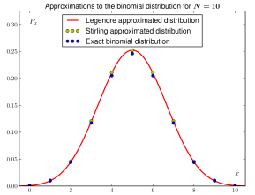
Figure 1: Comparison of the continuous distribution obtained by a Legendre transform (with finite size corrections) of the generating function, cf. equation (48), with the exact binomial distribution (44) for $N=10$. For a fair comparison one should perhaps compare the exact probability $P_{x}$ given by (44) with the average value of (48) over the interval $\left(x-\frac{1}{2},x+\frac{1}{2}\right)$. The result of making a Stirling approximation of the binomial coefficient is also shown. This approximation gives $P_{x}=0$ at the endpoints $x=0$ and $x=N$.

Consider the “partition function”

$$\text{e}^{f(p)}=2^{-N}\,\left(1+\text{e}^{p}\right)^{N}.$$ (43)

This actually is the generating function for the probability of $x$ heads in a sequence of $N$ independently flipped coins, corresponding to the probability

$$P_{x}\equiv\text{e}^{-u(x)}=2^{-N}\,\binom{N}{x},$$ (44)

but assume we don’t know that. We instead use the method above, with

$$f(p) =N\log\left(1+\text{e}^{p}\right)-N\log 2,$$ (45)

$$f^{\prime\prime}(p) =N\,\text{e}^{p}(1+\text{e}^{p})^{-2}.$$ (46)

From

$$x =\frac{d}{dp}\left[f(p)-\frac{1}{2}\log 2\pi f^{\prime\prime}(p)\right],$$

$$u(x) =px-\left[f(p)-\frac{1}{2}\log 2\pi f^{\prime\prime}(p)\right],$$

we find

$$p=\log\xi-\log(1-\xi),$$

where we have written $x=(N+1)\xi-\frac{1}{2}$ to simplify expressions, and

$$u(x) =(N+1)\left[\xi\log\xi+(1-\xi)\log(1-\xi)\right]$$

$$+{\textstyle\frac{1}{2}}\log 2\pi N+N\log 2.$$ (47)

This means that the discrete probability $P_{x}$ of equation (44) is approximated by a continuous distribution

$$\text{e}^{-u(x)}=2^{-N}\frac{1}{\sqrt{2\pi N}}\,\text{e}^{-(N+1)\left[\xi\log\xi+(1-\xi)\log(1-\xi)\right]},$$ (48)

which should be compared with the Stirling approximation to the binomial coefficient

$$2^{-N}\, \binom{N}{x}\approx 2^{-N}\frac{1}{\sqrt{2\pi N}}$$

$$\times\frac{1}{\sqrt{\chi(1-\chi)}}\text{e}^{-N\left[\chi\log\chi+(1-\chi)\log(1-\chi)\right]},$$ (49)

where $x=N\chi$. Comparisons between the exact distribution (44), its Stirling approximation (49), and the Legendre transformed approximation (48) are shown in Fig. 1 and 2.

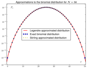
Figure 2: Comparison of the continuous distribution obtained by a Legendre transform (with finite size corrections) of the generating function, cf. equation (48), with the exact binomial distribution (44) for $N=50$. The result of making a Stirling approximation of the binomial coefficient is also shown. This approximation gives $P_{x}=0$ at the endpoints $x=0$ and $x=N$.

4 Estimating Frobenius coefficients by Legendre transform

We now use the results of the previous section for our main objective, to estimate the magnitude of the coefficients $a_{m}$. Here we will not consider the presence of logarithmic terms. Our basic hypothesis is that the sum (6) for large $|z|$ receives its main contribution from a relatively small range of $m$-values, at least for some phase values of $z$. Introduce quantities $u$ and $s(m)$ so that

$$x=\text{e}^{u},\quad|a_{m}|=\text{e}^{s(m)}.$$

Hence our hypothesis is that

$$\text{e}^{S(u)}\equiv\max_{\varphi}\psi(\text{e}^{u+i\varphi})\approx\sum_{m}\text{e}^{s(m)+(\nu+m)u},$$ (50)

with the main contribution to the sum coming from a relatively small range of $m$-values around a maximum value $\bar{m}$. The latter is defined so that $s^{\prime}(\bar{m})+u=0$, $s^{\prime\prime}(\bar{m})<0$. Now write $m=\bar{m}+\Delta m$, and approximate the sum (50) over $\Delta m$ by a gaussian integral. This gives

$$\text{e}^{S(u)}\approx\sqrt{{-2\pi}/{s^{\prime\prime}(\bar{m})}}\,\text{e}^{s(\bar{m})+(\nu+\bar{m})u}.$$

In summary, we have found the relations

$$u =-s^{\prime}(m),$$ (51)

$$S(u) =s(m)-(\nu+m)s^{\prime}(m)+\frac{1}{2}\log\left(\frac{2\pi}{-s^{\prime\prime}(m)}\right)$$

$$\equiv S_{0}(u)+\frac{1}{2}\log\left(\frac{2\pi}{-s^{\prime\prime}(m)}\right).$$ (52)

Compared with the discussion in the previous section we see that this is essentially a Legendre transformation between $s(m)$ and $S(u)$, but since there are some minor differences we repeat the derivation of the inverse transformation.

Consider a small change $u\to u+\delta u$. To maintain the maximum condition we must also make a small change $m\to m+\delta m$, with $\delta m=-{\delta u}/{s^{\prime\prime}(m)}$. I.e. $s^{\prime\prime}(m)=-u^{\prime}(m)$. This is consistent with the result of taking the $m$-derivative of equation (51). One further finds that $S_{0}(u)$ becomes

$$S_{0}(u+\delta u)=S_{0}(u)+S^{\prime}_{0}(u)\,\delta u+\frac{1}{2}S^{\prime\prime}_{0}(u)\,\delta u^{2}+\cdots$$

$$=s(m)+(\nu+m)u+(m+\nu)\,\delta u-\frac{1}{2s^{\prime\prime}(m)}\,\delta u^{2}+\cdots,$$

giving the relations

$$(m+\nu) =S^{\prime}_{0}(u),$$ (53)

$$s(m) =S_{0}(u)-uS^{\prime}_{0}(u),$$ (54)

$$s^{\prime\prime}(m) =-S^{\prime\prime}_{0}(u)^{-1}.$$ (55)

Equation (55) just says that $\left(dm/du\right)=\left(du/dm\right)^{-1}$. We are only able to compute $S(u)$ directly, not $S_{0}(u)$. However, they only differ by a logarithmic term, hence we will approximate $\log(-s^{\prime\prime}(m))=-\log S^{\prime\prime}_{0}(u)\approx-\log S^{\prime\prime}(u)$. This gives

$$S_{0}(u)\approx S(u)-\frac{1}{2}\log\left(2\pi\,S^{\prime\prime}(u)\right),$$ (56)

which can be used in equations (53–55) when we have computed $S(u)$.

5 WKB approximation

It remains to find $S(u)$. Here we will use the leading order WKB approximation to find a sufficiently accurate estimate. When $z=0$ is an ordinary point, i.e. when $\nu_{-}=0$, $\nu_{+}=1$, the leading order WKB solution to (5) is [12, 13, 14]

$$\psi(z)\approx\sqrt{Q_{0}/Q(z)}\exp\left({\frac{1}{s}}\int_{0}^{z}Q(t)\text{d}t\right),$$ (57)

where $Q^{2}(z)=\sum_{n=1}^{N}\text{v}_{n}z^{n-1}$, and $Q_{0}=Q(0)$. This represents a superposition of the solutions $\psi_{\pm}(z)$. The difference between the $\nu_{+}$ and $\nu_{-}$ solutions is at worst comparable to accuracy of our approximation; hence we will not distinguish between them.

When $z=0$ is a regular singular point we use the Langer corrected WKB approximation to obtain leading order solutions in the form

$$\psi_{\pm}(z) \approx z^{\nu_{\pm}}\sqrt{Q_{0}/Q(z)}\;\times$$

$$\exp\left(\pm\frac{1}{s}\int_{0}^{z}\frac{\text{d}t}{t}\left[\sqrt{Q^{2}(t)}-Q_{0}\right]\right).$$ (58)

Here $Q^{2}(z)=\frac{1}{4}s^{2}(\nu_{+}-\nu_{-})^{2}+\sum_{n=0}^{N}\text{v}_{n}z^{n+1}$, and $Q_{0}=Q(0)$. In equation (58) we distinguish between the $\nu_{+}$- and $\nu_{-}$-solutions, because the difference $\nu_{+}-\nu_{-}$ may in principle be large.

The WKB integrals must in general be done numerically, sometimes along curves in the complex plane. This requires careful attention to branch cuts. One must also take into account that the behaviour of the WKB solution may change from one exponential behaviour to another, due to the existence of Stokes lines [15]. We have observed that this sometimes can be explained as contributions from topologically different integrations paths. In this paper we will only give some examples where most of the calculations can be done analytically.

6 Examples

6.1 Anharmonic oscillators

Consider the equation

$$-\frac{\partial^{2}}{\partial y^{2}}\Psi(y)+\left(y^{2}+c^{2}\right)^{2}\Psi(y)=0,$$ (59)

for real $c$ so that $c^{2}\geq 0$. For large $y$ the typical solution behaves like

$$\Psi(y)\sim\text{e}^{\frac{1}{3}y^{3}+c^{2}y},$$ (60)

neglecting the slowly varying prefactor. For a given value of $|y|$ this is maximum along the positive real axis. Hence, with $x=y^{2}=\text{e}^{u}$, we find as a leading approximation

$$S(u)={\textstyle\frac{1}{3}}\left(\text{e}^{\frac{3}{2}u}+3c^{2}\text{e}^{\frac{1}{2}u}\right).$$

In this case the Frobenius series can be written

$$\Psi(y)=\sum_{m=0}^{\infty}a_{m}\,y^{2m+\nu}\equiv\sum_{m=0}^{\infty}A_{m}(y),$$ (61)

with $\nu=0,\;1$. Ignoring the $\log(S^{\prime\prime}(u))$-term in (53, 54, 56) we find

$${m} ={\textstyle\frac{1}{2}}\left(\text{e}^{\frac{3}{2}u}+c^{2}\,\text{e}^{\frac{1}{2}u}\right),$$ (62)

$$\log\left(\left|a_{{m}}\right|\right) =\left({\textstyle\frac{1}{3}}-{\textstyle\frac{1}{2}}u\right)\text{e}^{\frac{3}{2}u}+c^{2}\left(1-{\textstyle\frac{1}{2}}u\right)\text{e}^{\frac{1}{2}u}.$$ (63)

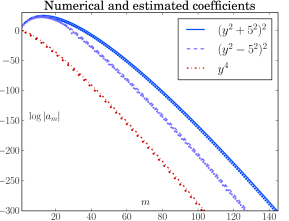
Figure 3: Comparison of numerical coefficients $a_{m}$ (points) with estimates (full-drawn lines) based on (62, 63) and (LABEL:m_DoubleWell). The estimates of $\log|a_{m}|$ are accurate up to corrections which depend logarithmically on $m$.

For $c=0$ an explicit representation is

$$\log|a_{m}|=\frac{2}{3}m\left(1-\log 2m\right).$$ (64)

This is plotted as the lower curve in figure 3. It fits satisfactory with the high-precision coefficients generated numerically, but there remains a correction which depends logarithmically on $m$. For nonzero $c$ the parametric representation provides equally good results, as shown by the upper curve in figure 3.

The conclusion of this example is that for a fixed (large) $x$ we expect the largest term of the power series to be

$$\mathop{\text{max}}_{m}|A_{m}(x)|\sim\text{e}^{\frac{1}{3}(x^{3/2}+3c^{2}x^{1/2})},$$ (65)

neglecting a slowly varying prefactor. Further, the maximum should occur at

$$m\approx{\textstyle\frac{1}{2}}\left(x^{3/2}+c^{2}x^{1/2}\right).$$ (66)

Finally, estimates like equation (64) for the coefficients $a_{m}$ may be used to predict how many terms ${\cal M}$ we must sum to evaluate $\psi(x)$ to a given precision $P$, based on the stopping criterium

$$|a_{\cal M}|\,x^{\cal{M}}\leq 10^{-P}.$$ (67)

As can be seen in figure 4 the agreement with the actual number of terms used by our evaluation routine is good, in particular for high precision $P$. But keep in mind that a logarithmic scale makes it easier for a comparison to look good.

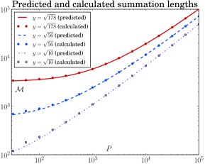
Figure 4: This figure compares the a priori prediction, based on equation (64), of the number of terms ${\cal M}$ which must be summed in order to evaluate $\Psi(y)$ for $c=0$ to a desired precision $P$, with the actual number of terms computed by the numerical routine [6].

Next consider the logarithmic corrections. Including the prefactor of equation (60) changes $S(u)$ by an amount

$$\Delta S(u)=-\frac{1}{2}\log\left(\text{e}^{u}+c^{2}\right).$$ (68)

Including the $\log(S^{\prime\prime}(u))$-term in the relation between $S(u)$ and $S_{0}(u)$ changes $S_{0}$ by an additional amount

$$\Delta S_{0}(u)=-\frac{1}{2}\log\left(\frac{3}{4}\text{e}^{\frac{3}{2}u}+\frac{1}{4}c^{2}\,\text{e}^{\frac{1}{2}u}\right).$$ (69)

For $c^{2}=0$ this changes the relation (64) to

$$\log|a_{m}|=\frac{1}{3}\left(2m+{5}/{2}\right)\left(1-\log\left(2m+{5}/{2}\right)\right).$$ (70)

For $|a_{m}|$ this essentially corresponds to a factor $m^{-5/6}$.

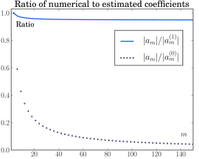
Figure 5: This figure shows the ratio between the computed coefficients $a_{m}$ and the crude prediction (64) (labelled $|a^{(0)}_{m}|$) and the logarithmically corrected prediction (70) (labelled $|a^{(1)}_{m}|$). For easy comparison we have in both cases adjusted an overall constant such that the ratio is unity for $m=3$.

6.2 Double well oscillators

The same procedure also work for the equation

$$-\frac{\partial^{2}}{\partial y^{2}}\Psi(y)+\left(y^{2}-c^{2}\right)^{2}\Psi(y)=0,$$ (71)

which however is a little more challenging since the maximum value of $|\Psi(y\text{e}^{\text{i}\varphi}|$ sometimes occur for $\varphi\neq 0$, i.e. for complex arguments.

For large $y$ the typical solution behaves like

$$\Psi(y)\sim\text{e}^{\frac{1}{3}y^{3}-c^{2}y},$$ (72)

neglecting the slowly varying prefactor. Equation (71) can be transformed to the form (5) by introducing $x=y^{2}$, $\Psi(y)=\psi(x)$. Hence, with $x=y^{2}=\text{e}^{u}$

$$S(u)=\mathop{\text{max}}_{\varphi}{\textstyle\frac{1}{3}}\text{Re}\left(\text{e}^{\frac{3}{2}(u+\text{i}\varphi)}-3c^{2}\text{e}^{\frac{1}{2}(u+\text{i}\varphi)}\right).$$

The maximum occurs for $\cos\frac{1}{2}\varphi=-\frac{1}{2}\left(1+c^{2}\,\text{e}^{-u}\right)^{1/2}$ when $\text{e}^{u}\geq\frac{1}{3}c^{2}$, and for $\cos\frac{1}{2}\varphi=-1$ otherwise. This gives

$$S(u)=\left\{\begin{array}[]{cc}{\textstyle c^{2}\text{e}^{u/2}-\frac{1}{3}\text{e}^{3u/2}}&\text{for $e^{u}\leq\frac{1}{3}c^{2}$,}\\[2.15277pt] {\textstyle\frac{1}{3}}(\text{e}^{u}+c^{2})^{3/2}&\text{for $e^{u}\geq\frac{1}{3}c^{2}$.}\end{array}\right.$$ (73)

This implies that

$$\bar{m} =\left\{\begin{array}[]{lc}\frac{1}{2}\text{e}^{u/2}\left(c^{2}-e^{u}\right)&\text{for $e^{u}\leq\frac{1}{3}c^{2}$,}\\[1.72221pt] {\textstyle\frac{1}{2}}\text{e}^{u}\,\left(\text{e}^{u}+c^{2}\right)^{1/2}&\!\!\!\text{for $e^{u}\geq\frac{1}{3}c^{2}$},\end{array}\right.$$ (76)

$$\log\left(\left|a_{\bar{m}}\right|\right) =$$

$$\left\{\begin{array}[]{cc}\left(1\!-\!\frac{1}{2}u\right)c^{2}\text{e}^{u/2}-\left(\frac{1}{3}-\frac{1}{2}u\right)\text{e}^{3u/2}&\text{for $e^{u}\leq\frac{1}{3}c^{2}$,}\\[1.72221pt] \left[\left({\textstyle\frac{1}{3}}\!-\!{\textstyle\frac{1}{2}}u\right)\text{e}^{u}+{\textstyle\frac{1}{3}}c^{2}\right]\left(\text{e}^{u}+c^{2}\right)^{1/2}&\text{for $e^{u}\geq\frac{1}{3}c^{2}$}.\end{array}\right.$$ (80)

This representation compares fairly well with the numerically generated coefficients, as shown by the middle curve in figure 3. However, in this case the coefficients $a_{m}$ have a local oscillating behaviour. The representation (LABEL:m_DoubleWell) should be interpreted as the local amplitude of this oscillation.

The conclusion of this example is that we expect the largest term of the power series to be term of the series to be

$$\mathop{\text{max}}_{m}|A_{m}(x)|\sim\text{e}^{\frac{1}{3}(x+c^{2})^{3/2}},$$ (81)

neglecting the slowly varying prefactor. Further, the maximum should occur at

$$m\approx{\textstyle\frac{1}{2}}x\left(x+c^{2}\right)^{1/2}\approx{\textstyle\frac{1}{2}}x^{3/2}+{\textstyle\frac{1}{4}}c^{2}x^{1/2}.$$ (82)

7 Conclusion

As illustrated in this contribution the coefficients of Frobenius series can be predicted to surprisingly high accuracy by use of Legendre transformations and lowest order WKB approximations. We have also tested the validity of the method on many other cases.

References

- [1] Philip M. Morse and Herman Feshbach, Methods of Theoretical Physics, Part I, pp. 508–515, McGraw-Hill (1953)
- [2] Philip M. Morse and Herman Feshbach, Methods of Theoretical Physics, Part I, p. 663, McGraw-Hill (1953)
- [3] E.T. Whittaker and A.N. Watson, A course of MODERN ANALYSIS, 4th ed, reprinted by Cambridge University Press (2002)
- [4] A. Mushtaq, A. Noreen, K. Olaussen and I. Øverbø, Very-high-precision solutions of a class of Schrödinger type equations, Computer Physics Communications, 182, no. 9, pp. 1810-1813 (2011)
- [5] A. Noreen, K. Olaussen, Very-high-precision normalized eigenfunctions for a class of Schrödinger type equations, Proceedings of World Academy of Science, Engineering and Technology, 76, pp. 831-836 (2011)
- [6] A. Noreen, K. Olaussen, High precision series solution of differential equations: Ordinary and regular singular point of second order ODEs, Computer Physics Communications, 183, no. 10, pp. 2291-2297 (2012)
- [7] F.G. Frobenius, Über die Integration der linearen Differentialgleichungen durch Reihen, Journal für die reine und angewandte Mathematik, 76, p. 214–235 (1873)
-
[8]
A. Noreen, K. Olaussen, Estimating Coefficients of Frobenius Series by
Legendre Transform and WKB Approximation, Lecture Notes in Engineering and Computer Science: Proceedings of The World Congress on Engineering 2012, WCE 2012, 4-6 July, 2012, London, U.K., pp. 789-791. - [9] R.T Rockafellar, Convex Analysis paperback ed., Princeton University Press (1996)
- [10] K. Huang, Statistical Mechanics 2nd ed., John Wiley & Sons (1987)
- [11] R. K. P. Zia, Edward F. Redish, and Susan R. McKay, Making Sense of the Legendre Transform, arXiv.org//0806.1147 (2008)
- [12] L.I. Schiff, Quantum Mechanics, Third Edition, section 34, McGraw-Hill (1968)
- [13] H. Kroemer, Quantum Mechanics: for engineering, materials science, and applied physics, Chapter 6, Prentice Hall (1994)
- [14] C.M Bender and S.A. Orszag, Advanced Mathematical Methods for Scientists and Engineers, Chapter 10, McGraw-Hill (1978)
- [15] W.H. Furry, Two notes on Phase-Integral Methods, Physical Review 71 pp. 360–371 (1947)