Revealing a strongly reddened, faint active galactic nucleus population by stacking deep co-added images

Abstract

More than half of the sources identified by recent radio sky surveys have not been detected by wide-field optical surveys. We present a study based on our co-added image stacking technique, in which our aim is to detect the optical emission from unresolved, isolated radio sources of the Very Large Array (VLA) Faint Images of the Radio Sky at Twenty-cm (FIRST) survey that have no identified optical counterparts in the Sloan Digital Sky Survey (SDSS) Stripe 82 co-added data set. From the FIRST catalogue, 2116 such radio point sources were selected, and cut-out images, centred on the FIRST coordinates, were generated from the Stripe 82 images. The already co-added cut-outs were stacked once again to obtain images of high signal-to-noise ratio, in the hope that optical emission from the radio sources would become detectable. Multiple stacks were generated, based on the radio luminosity of the point sources. The resulting stacked images show central peaks similar to point sources. The peaks have very red colours with steep optical spectral energy distributions. We have found that the optical spectral index $\alpha_{\nu}$ falls in the range $-2.9\leq\alpha_{\nu}\leq-2.2$ ($S_{\nu}\propto\nu^{\alpha_{\nu}}$), depending only weakly on the radio flux. The total integration times of the stacks are between $270$ and $300$ h, and the corresponding $5\sigma$ detection limit is estimated to be about $m_{r}\simeq 26.6$ mag. We argue that the detected light is mainly from the central regions of dust-reddened Type 1 active galactic nuclei. Dust-reddened quasars might represent an early phase of quasar evolution, and thus they can also give us an insight into the formation of massive galaxies. The data used in the paper are available on-line at http://www.vo.elte.hu/doublestacking.

1 Introduction

A significant fraction of sources that have been detected in recent deep radio sky surveys have not yet been detected in the optical wavelength regime by wide field surveys. From the about $10^{6}$ objects identified by the Very Large Array (VLA) Faint Images of the Radio Sky at Twenty-cm (FIRST) survey (Becker et al., 1995; White et al., 1997), only approximately $30$ per cent have optical counterparts in the legacy Sloan Digital Sky Survey (SDSS; York et al., 2000; Ivezić et al., 2002) at a limiting magnitude of $r\sim 22.2$. We estimate that for the SDSS Stripe 82 co-added survey, which is about $1.8$ mag deeper (Abazajian et al., 2009), this detection ratio is about $42$ per cent.

The nature of the optically undetected fraction has been the subject of debate for many years. Recent studies have shown that there exists a significant population of reddened radio-selected quasars (Webster et al., 1995; Cutri et al., 2001; Gregg et al., 2002; Richards et al., 2003; White et al., 2003; Glikman et al., 2004; Martínez-Sansigre et al., 2005; Glikman et al., 2007). According to the generally accepted unification model (e.g. Antonucci, 1993), a likely explanation for the low optical luminosity of these quasars is that their central engines are obscured by an optically thick dust torus.

In this paper, we use a new image stacking technique to investigate the average optical properties of unresolved faint point sources from the VLA FIRST survey that have no detected optical counterparts in the SDSS Stripe 82 (equatorial stripe) co-added data set (Abazajian et al., 2009).We call our technique deep co-add stacking (DCS) because we stack images that have already been co-added from multiple observations of the SDSS equatorial stripe. In our technique, we put strong emphasis on accurate background estimation and on correcting for selection effects.

1.1 Image stacking

Co-adding repeated observations and stacking of images of different, but similar objects can be used to extend the limiting magnitude and surface brightness limits of surveys. When stacking images of different extended sources with varying apparent sizes – depending on the specific needs – cut-out images are made, which can be rotated, resized and/or otherwise scaled together to make the individual objects overlap. Stacking increases the signal-to-noise ratio of the images by reducing the photon noise. For undetected sources, stacking can be successfully used to reveal an average image of extremely faint sources that otherwise would be beyond the detection limits of the instruments. The individual objects must be similar to each other in order to be able to give a physical interpretation to the average images. The application of image stacking is limited by a couple of factors, of which the thermal and read-out noise of the detectors are the most important. However, modern detector technology makes it possible to stack hundreds of images together, without significant systematic background noise in the results.

One important disadvantage of image stacking is its limited capability for statistical analysis. In the optical wavelength regime, usually only one or a few stacked images per band are obtained from the individual cut-outs. Bootstrapping techniques can be used to determine the variance of the measured properties of the stacked images by sacrificing the surface brightness depth and signal-to-noise ratio.

When we are interested in faint objects only, it is important to exclude those pixels of the individual cut-outs from stacking that are brighter than a carefully determined threshold; otherwise, the strong signal from the brighter sources or stray light from nearby bright sources would wash away the very weak signal of the faint object. Fine-tuned masking techniques are required to address this problem, as we show in Section 3.2.

Previously, image stacking has been used successfully to recover the undetected light from objects that are visible in a given wavelength range but are too faint in another to detect them directly. White et al. (2007) stacked VLA FIRST images of optically identified quasars, and investigated the radio properties (the correlation between radio and optical luminosities, radio loudness) of the sample. Hodge et al. (2008) identified the faint radio emission from a diverse sample of quiescent (optically unclassifiable) galaxies from the SDSS by stacking their FIRST radio images. They showed that the radio emission from these galaxies can be related to their star formation rate, or a significant part of these galaxies might harbour quiescent active galactic nuclei (AGNs) in their cores and their activity is related to the stellar mass. They continued their analysis by stacking radio images of luminous red galaxies (LRGs) from the SDSS. They showed that low radio luminosity AGNs (with $1400$ MHz flux densities in the $10\leq S_{\text{int},1400}\leq 100$ $\mu$Jy range) are characteristic of the LRG population, and that an evolution of the nuclear activity is apparent for redshifts in the range $0.45<z<0.6$ (Hodge et al., 2009). Radio contribution by star formation was ruled out by sample selection (i.e. LRGs are passive galaxies with no significant star formation).

Another use of the stacking method is the detection of faint haloes of extended objects. Zibetti et al. (2004) stacked SDSS optical images of edge-on disc galaxies to detect their stellar halo components, and they reached a surface brightness level as low as $\mu_{r}\simeq 31$ mag arcsec^-2. Later, they analysed the radial profile of intracluster light by stacking the SDSS images of $683$ galaxy clusters. They identified faint emission from intergalactic stars as far as $700$ kpc from the centres of the clusters, by pushing the surface brightness limit of the stacked images to $\mu_{r}\simeq 27.5-30$ mag arcsec^-2 in the SDSS r-band (Zibetti et al., 2005). Also, Zibetti et al. (2007) applied their technique to reveal light from Mgii absorbers. Hathi et al. (2008) used image stacking to determine the average properties of the surface brightness profiles of very distant, compact galaxies in the Hubble Deep Field. Bergvall et al. (2010) detected the extended red haloes of low surface brightness SDSS galaxies.Most recently, Tal & van Dokkum (2011) have investigated the faint stellar haloes of LRGs by stacking SDSS images. They have found that stellar light in massive elliptical galaxies can be traced out to about a radius of $100$ kpc.

An interesting similarity of these SDSS-based studies is that the stacked images show extremely red colours. According to Zibetti et al. (2004) the $r-i$ colours of the stellar haloes of the galaxies reach up to about $0.8$ mag, which is attributed to very old and/or metal-abundant stellar populations. As an explanation, for the case of edge-on disc galaxies, de Jong (2008) has provided evidence that the anomalous halo colours are at least partly a result of the underestimated effect of the extended tails of the point spread function (PSF).

1.2 Radio–optical cross-identification

Cross-identification of radio sources with their optical counterparts is a challenging problem because of the complex morphology of radio galaxies. Many studies have previously investigated the possibilities of automatic radio–optical cross-identification and the connections between the optical and radio properties of extragalactic objects. McMahon et al. (2002) automatically identified the optical counterparts of the FIRST radio sources in the Cambridge Automated Plate Measurement (APM) scans of the First Palomar Observatory Sky Survey (POSS-I) plates, and they found about $70.000$ matches. According to them, in the case of the aforementioned catalogues, positional coincidence is enough to cross-identify radio point sources with optical sources at false-positive levels lower than 5 per cent when an association radius of 2 arcsec is used. This false-positive rate is, of course, only for the particular combination of catalogues of that study. The rate depends on the astrometrical accuracy of the catalogues and the density of sources. McMahon et al. (2002) also addressed the cross-identification of double radio sources with their optically observable counterparts. They found that an optical counterpart is likely to be found halfway between the components of the radio source pairs.

1.3 Origins of the unresolved radio emission

In Section 2, we construct a sample of optically undetected, unresolved radio sources with integrated $1400$ MHz radio flux above $S_{1400}\geq 1$ mJy. We consider several types of radio sources that can appear unresolved in the VLA FIRST images: galactic pulsars, radio stars, hotspots of radio jets associated with the outer regions of radio galaxies and AGNs (including quasars).

A flux density limit of $1$ mJy is useful to separate AGNs from low redshift starburst galaxies. This limit is sufficiently bright to exclude most of the starburst galaxies, and yet faint enough to permit high redshift AGNs and classical radio galaxies (Windhorst et al., 1985; Hopkins et al., 2000). The 1-mJy limit was used by Waddington et al. (2001), who compiled the Leiden–Berkeley Deep Survey (LBDS) Hercules sample, which is still the largest optically complete sample of mJy radio sources at $1400$ MHz.

Because we restrict our analysis to the area covered by the SDSS Stripe 82 ($-50^{\circ}\leq\alpha\leq 59^{\circ}$, $|\delta|\leq 1.26^{\circ}$), the high galactic latitude and the relatively high selection limit on the radio flux make it very unlikely that the resulting point sources are pulsars. For example, the comprehensive Australia Telescope National Facility (ATNF) pulsar catalogue (Manchester et al., 2005) contains only two pulsars within the footprint of Stripe 82. This number is negligible compared to the more than $20.000$ unresolved radio objects that are catalogued in the VLA FIRST data set within the same footprint.

According to Helfand et al. (1999), there are 26 known radio stars brighter than $0.7$ mJy at $1400$ MHz discovered in the FIRST survey, from which only three sources lie in the Stripe 82 footprint. Therefore, it is very unlikely that our optically undetected sample of 2116 objects contains any radio stars.

Hotspots of radio galaxy jets might also appear as point sources in FIRST images. They are almost always associated with an easily detectable nearby elliptical galaxy and they tend to appear in pairs, on both sides of the galaxies. We have identified many sources that are very good candidates for such hotspots, but we have excluded them from the present analysis using a method described in Section 2.1.

The fourth type of objects that appear as unresolved, isolated radio sources are the central regions of supermassive black holes currently accreting matter. In Section 6, we argue that we detect the optical light from this type of sources.

1.4 Reddened radio-loud quasars

According to the widely accepted AGN unification scheme (for a review, see Antonucci, 1993; Urry & Padovani, 1995, and references therein), AGNs are divided into two main classes based on their optical properties. Type 1 AGNs have both broad and narrow emission lines and show blue optical continua. This implies that the central regions of these objects are observed directly with no significant quantity of obscuring material along the light of sight. However, Type 2 sources show red optical spectra and narrow emission lines only. It is believed that Type 2 AGNs are viewed from such directions that the dense dust clouds surrounding the central engines fall into the line of sight and obscure much of the visible light coming from the accretion discs. The broad emission lines are associated with the central regions of the accretion discs, where high velocity motion is responsible for the broadening of the lines. Polarimetric studies have revealed that weak, highly polarized broad emission lines are also detectable in the spectra of Type 2 AGNs. These highly polarized lines are attributed to the light that originates from the central regions but is reflected from gas clouds at greater distances from the centres.

It has been demonstrated previously that there exists a strongly reddened population of quasars, which are often missed by the conservative quasar selection criteria of optical sky surveys. Ivezić et al. (2002) presented a very comprehensive study about the optical and radio properties of positionally matched FIRST and SDSS sources. By analysing the distribution of quasars, they pointed out that the existence of a significant population of highly obscured quasars that are visible in FIRST but not in SDSS cannot be ruled out by the data. Richards et al. (2003) estimated that about 10 per cent of the dust-reddened quasars are missing from the SDSS catalogue because of selection effects. They also estimated that the fraction of broad absorption line (BAL) quasars rises with redder colour and can reach 20 per cent for reddened quasars. In the case of BAL quasars, the BALs are most likely to originate from the fast moving dust expelled from the central regions by the strong wind of the nucleus (Hazard et al., 1984; Weymann et al., 1991; Sprayberry & Foltz, 1992; Ogle et al., 1999; Schmidt & Hines, 1999; Becker et al., 2000; Hall et al., 2002; Trump et al., 2006).

Glikman et al. (2007) have confirmed that the selection of quasars by infrared colours yields a significantly redder quasar population than selection based on optical surveys. They have also reported, based on two-frequency radio observations, that the red colours of these quasars are more likely to be a result of extinction by dust rather than enhanced synchrotron emission. They have found that the intrinsic extinction values of these reddened quasars can reach as high as $E(B-V)\simeq 2.5$ mag.

Certain models suggest that AGNs are turned on by galaxy mergers and that they spend a significant time obscured by the dust that originates from the merging host galaxies (Sanders et al., 1988; Hopkins et al., 2005). In this phase, the AGNs have high intrinsic luminosities, but they appear as heavily reddened Type 1s (or ultraluminous infrared galaxies) because of strong obscuration by the dust of the hosts. The unobscured quasars become visible once the radiation from the central engines wipes out the obscuring material.

Urrutia et al. (2009) have investigated the properties of heavily reddened quasars of a sample compiled from FIRST, the Two- Micron All-Sky Survey (2MASS; Skrutskie et al., 2006) and SDSS. The majority of their sample was spectroscopically confirmed, and they found that a quasar population with high intrinsic extinction does exist far from the traditional photometric quasar selection criteria. Urrutia et al. (2009) measured the reddening values to be in the range $0.1<E(B-V)<1$ mag, where the higher values are more consistent with obscuration by the host galaxies rather than being a result of the dust torus surrounding the central engines. They have also found that these quasars are likely to show BALs of elements at low ionization states. This observation suggests that these AGNs are at an early period of their active cycles, when strong winds driving the dust out from the central regions cause the BALs.

For a comprehensive review of the spectral energy distributions (SEDs) of Type 1 quasars, see Richards et al. (2006).

1.5 Structure of the paper

In Section 2, we describe the radio object sample selection method, and the source of the optical imaging data. We give details of the image stacking algorithm in Section 3, and we present the results of the analysis – including photometry, SED and radial surface brightness profiles of the stacked objects – in Section 5. Finally, in Section 6, we discuss the optical and infrared properties of our sample.

We use the concordance flat $\Lambda$ cold dark matter (CDM) cosmology throughout this paper, with parameters of $H_{0}=71$ km s^-1 Mpc^-1, $\Omega_{M}=0.27$ and $\Omega_{\Lambda}=0.73$.

We have developed our own software tools, written in IDL, to generate cut-out images and masks, and for the entire image stacking process. The code is available from the authors on request.

2 Data

For the present analysis, we use $1400$ MHz radio data from the VLA FIRST survey (Becker et al., 1995) and $u$, $g$, $r$, $i$ and $z$-band optical images from the SDSS Stripe 82 co-added data set (Abazajian et al., 2009). The aim of our analysis is to detect the faint optical emission of sources that are individually undetected in the optical, but which have significant emission in the radio. We choose our sample selection criteria according to the requirements detailed in the following two subsections.

2.1 Sample selection from the FIRST catalogue

We only select those FIRST objects that are within the SDSS equatorial stripe footprint ($-50^{\circ}\leq\alpha\leq 59^{\circ}$, $|\delta|\leq 1.26^{\circ}$). Objects are required to be compact radio sources, i.e. point-like without any extended radio features. The FIRST catalogue assigns a side-lobe probability $P_{S}$ to each object based on oblique decision tree classifiers (refer to the FIRST web-site for details). We require that the side-lobe probability must be less than $P_{S}\leq 0.1$. In addition, the integrated $1400$ MHz fluxes of the objects must be higher than $S_{\text{int},1400}=1$ mJy. We visually inspect all automatically selected sources, as described in Section 2.2.

Figure 1: Pair-correlation function of 6019 FIRST radio point sources brighter than $S_{\textrm{int},1400}\geq 1$ mJy, plotted for small separations only. The reason behind the strong correlation at very small angles is that multiple point sources are likely to be associated with the same radio galaxy. The vertical dashed line indicates our $1.5$ arcmin limit on the minimum separation from any other radio sources.

In Fig. 1, the angular pair-correlation function of the FIRST radio point sources is plotted for small separations. A strong correlation at very small angles is clearly visible, but the function becomes flat above $1.5$ arcmin. This behaviour originates from the simple fact that radio galaxies have complex morphologies with many bright features: the multiple lobes and hotspots of radio galaxies are likely to appear as double or multiple associations of unresolved sources in the FIRST images that are close to each other. In most cases, the optical counterparts of these galaxies are easily identifiable in the proximity of the radio sources. In order to make sure that only isolated sources are included in the sample, we consider the angular pair-correlation function of them, and further restrict the selection conditions to exclude radio sources with another close radio companion within $1.5$ arcmin. This criterion is though to effectively exclude most point sources that are associated with optically resolved radio galaxies.

Because we are looking for compact radio sources with no clearly identified optical counterparts, in the analysis we only include those radio sources that do not have any matches in the SDSS Stripe82 co-added catalogue within $3$ arcsec. This condition is much less restrictive than the typical astrometric error of SDSS, which is about $0.1$ arcsec (Stoughton et al., 2002), but it is strict enough to exclude any false positive matches. It also excludes extended radio sources with small diameters that might show an offset of a few arcsec between the optical and radio source positions. This value is chosen because practically all true SDSS–FIRST matches have smaller separations than $3$ arcsec (Ivezić et al., 2002).

2.2 Visual inspection of the images

After applying the former criteria, 2626 sources remain. We identified these radio sources in the Deep VLA Stripe 82 catalogue (Hodge et al., 2011) which has double the resolution and about three times the signal-to-noise ratio of the FIRST survey. Although the deeper survey does not cover the entire Stripe 82 region (only about 120 square degrees of the total 280 square degrees, 43 per cent), we still can use the deeper catalogue to verify the efficiency of the selection criteria we used to filter the FIRST data set. We are especially interested whether radio point sources can be segregated from extended sources based solely on the information available in the lower resolution FIRST catalogue. Therefore, we visually inspect the FIRST, Deep VLA and SDSS Stripe 82 images of all previously selected sources.

First of all, we exclude all radio objects if the corresponding optical frames are visibly affected by scattered light from nearby bright stars. The number of these objects amounts to about 180. In a few cases, we have to exclude radio objects because they overlap with the outer regions of very bright, extended galaxies.

About 10 per cent of the automatically selected FIRST objects is rejected during visual inspection because they clearly show resolved features or appear very faint and different from the average FIRST PSF.

Next, we compare the FIRST and Deep VLA images of those objects which were observed during both surveys. While all objects appear pointlike in the FIRST images (although some show a slight eccentricity), about 4 per cent of the FIRST point sources are clearly resolved into radio galaxy features in the deeper and higher resolution VLA survey. Unfortunately, there appears to be no way to identify the resolved sources based solely on their FIRST catalogue properties. Hence, exclusion of radio objects that become resolved at higher resolution is only possible in one half of the sample.

R. A. J2000		Dec. J2000		$S_{\text{int},1400}$		rms flux
[deg]		[deg]		[mJy]		[mJy/beam]
331.	2879944	1.	2256938	11.	74	0.	150
353.	8881836	1.	2255382	2.	80	0.	143
327.	1674805	1.	2590889	5.	52	0.	148
353.	0435486	1.	1830354	18.	99	0.	147
37.	0628471	1.	1827827	2.	82	0.	138
18.	8434620	1.	1813327	1.	10	0.	145
356.	9854126	1.	1412108	14.	33	0.	136

Table 1: Sources of the final DCS sample. (The entire table is available in machine-readable form at http://www.vo.elte.hu/doublestacking. A portion is shown here.)

$S_{\textrm{int},1400}$	median flux	$\sigma_{S}$	$N$	$t_{\text{exp}}$
$[\text{mJy}]$	$[\text{mJy}]$	$[\text{mJy}]$		$[\text{h}]$
$1$ – $2$	1.45	0.28	709	290
$2$ – $4$	2.71	0.54	653	270
$>4$	7.61	26.1	754	300
Total	2.78	16.7	2116	860

Table 2: Distribution of the DCS sources by subsamples. $S_{\textrm{int},1400}$ is the $1400$ MHz flux density interval of the bin; $\sigma_{S}$ is the variance of the flux density, $N$ is the number of the sources of each subsample; and $t_{\text{exp}}$ the total effective exposure time of the stacked optical images.

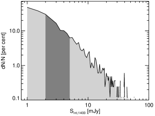
Figure 2: Distribution of the radio flux $S_{\text{int},1400}$ of the DCS sample. The grey areas indicate the three subsamples. light grey on the left: $1-2$ mJy; dark grey: $2-4$ mJy; light grey on the right: $>4$ mJy.

To select a radio source we required that it should be at least $1.5$ arcmin away from any other FIRST radio sources. When looking at the deeper radio survey images, objects of low radio brightness are apparent within $1.5$ arcmin in a few cases. Also, a very few objects detected in the FIRST survey are missing from the Deep VLA images. We attribute these false detections to glitches in the FIRST observations.

By looking at the higher-quality Deep VLA images, it is estimated that about $9$ per cent of the FIRST objects would be excluded at the depth of the Deep VLA observations. However, we have found that the exclusion or inclusion of these objects does not modify our final findings significantly; the difference in the measured fluxes is less than 5 per cent, which is in the range of the estimated error value. Although it can only be done for half of the data set, we still decide to exclude them from our final stacks.

2.3 Subsample definitions

The final, deep co-add stack (DCS) sample consists of 2116 objects, listed in Table 1. The sources are grouped into three, roughly equal cardinality subsamples based on their integrated apparent radio flux densities $S_{\text{int},1400}$. The size of the subsamples make it possible to generate stacks with high enough signal-to-noise ratio. The definitions of the subsamples are based on apparent flux because there are no redshift estimates available for the sample. Still, we can expect to see some dependence of the derived parameters on the apparent radio flux at the end of the analysis if the objects lie in a relatively narrow redshift range (i.e. a correlation between apparent and absolute radio luminosities exists).

Table 2 summarizes the properties of the three DCS subsamples. The distribution of the radio fluxes is plotted in Fig. 2.

2.4 SDSS co-added images

For the stacking, we use the SDSS equatorial stripe co-added imaging data to create cut-outs centred on the selected DCS source coordinates. The SDSS Stripe 82 images were co-added from about $20$–$40$ individual exposures (Abazajian et al., 2009). Each exposure took $54$ s and the resulting catalogue has an estimated $r$-band magnitude limit of about $r\lesssim 24$ mag, which is about one magnitude deeper than the rest of SDSS (Gunn et al., 1998).

3 Image stacking

3.1 Cut-outs

The DCS sample consists of radio sources with optical emissions below the detection limit of the SDSS Stripe 82 co-added catalogue. To reveal the average undetected light from these sources, first we generate cut-out images from the already co-added Stripe 82 images centred on the radio coordinates. Cut-outs of the size 200 by 200 pixels are made, which is equivalent to $80$ by $80$ arcsec at the resolution of SDSS. Cut-out image examples with radio flux contour overlays are presented in Fig. 3.

Because the background has already been subtracted from the images during the co-addition, the cut-out images should have sky levels of 0. Later, we show that this is not the case. In Section 3.4, we introduce a technique to re-estimate the zero level of the cutouts using an algorithm based on using cut-outs taken at random coordinates.

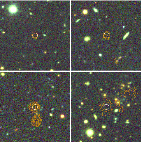
Figure 3: Sample cut-out images from the SDSS equatorial stripe (Stripe 82) co-added survey with $1400$ MHz radio flux contour overlays from FIRST. The top two images are examples of simple, isolated radio point sources, while the lower two ones show radio galaxies with more complex radio features. Only the top left object contributes our sample, the others (including the top right one) are excluded by the criterion which requires that no other radio objects should be in a $1.5$ arcmin radius of a given point source. The images are 80 arcsec wide on the side. The white circles have 3 arcsec radii. The contour levels are $0.4$, $0.65$, $1.0$, $1.45$, $2.0$, $2.65$, $3.4$, $4.25$, $5.2$, $6.25$, $7.4$ mJy beam^-1.

3.2 Masking

A significant portion of the pixels of the 200 by 200 Stripe 82 cut-outs is from bright objects that are out of our interest. Also, very frequently, stray light from nearby, bright ($m_{i}<16$ mag) stars contaminates the entire image, but light from interstellar clouds of the Milky Way can also be seen in some of the cut-outs. In order to reveal the very weak signal from the undetected sources, we have to exclude bright pixels efficiently. Our masking algorithm is based on a histogram cutting technique as described below.

3.2.1 Bright objects

The $1.5$ arcmin limit on the closest radio source implicitly assures that no associated radio galaxies will appear in the images (c.f. Section 2.1). Also, the condition that the selected radio sources have to be further away than $3$ arcsec from any detected optical sources ensures that there will be no readily visible optical sources in the centres of the cut-out images. However, outside the $3$ arcsec radius there can be numerous objects that have to be masked out before stacking the cut-outs together, otherwise the weak signal from the centres would not be detectable.

3.2.2 The masking algorithm

First, we have to determine the pixel values above which pixels should be rejected. Setting the right value for the masking threshold is crucial for the stacking to be successful. The values should be chosen in such a way that all pixels belonging to readily detectable objects are masked, while sky pixels and pixels of undetectable faint objects are kept.

Figure 4: Histograms illustrating the steps of our masking algorithm. Note the logarithmic vertical scale. a) Histogram of the pixel values of a single, typical SDSS Stripe 82 co-added frame. b) Histogram of the same frame convolved with a circular top-hat kernel with a radius of $1$ arcsec. c) Histogram of the frame after applying the mask (solid line). The unmasked histogram is indicated with a dotted line. The solid vertical lines are at the mean, the dashed lines are at the $\pm 1\sigma$ position of the original distribution. See the text for more details.

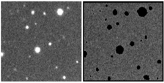
Figure 5: Left: a sample cut-out image from the stack. Right: The same image overlaid with the mask (shown as black regions).

The histogram of the pixel values of a single Stripe 82 co-added frame is plotted in panel (a) of Fig. 4 as an example. Because we use co-added images, the sky level is already subtracted at least to first order. This can be seen clearly from the figure; the histogram peaks nearly at zero and background pixels can have both positive and negative values. The negative part of the histogram is completely dominated by the noise of the sky pixels, while the longer tail towards the bright pixels comes from the objects.

The masking process is carried out in four steps, as follows.

1. First, we determine the masking threshold. We fit the negative side of the distribution of pixel values with a Gaussian function, assuming that the distribution of the background pixels is symmetric around zero. The masking threshold is then set to be at the $1\sigma$ variance of the fitted Gaussian. We indicate the value of the mean and $\pm 1\sigma$ as vertical lines in the panels of Fig. 4.

   A higher threshold would let more bright pixels into the statistics, which would increase the contribution of light from unwanted objects to the background, resulting in lower contrast stacks. However, if the value of the threshold was too low, we would filter out much of the light from the interesting faint sources themselves and render them undetectable in the stacks. We have found that the $1\sigma$ threshold yields a good balance between contrast and detectability. In Section 4.2, we show that changing this value slightly does not affect the final results.

   The $\sigma$ values for each SDSS band are determined from the pixel distribution of the whole ensemble of cut-outs, and the same values are used throughout the analysis.

2. Secondly, we make smoothed images from the original cutouts. This step is important because the imaged sources have diffuse edges. Therefore, masks derived directly from the cut-out images by cutting at the masking threshold would not be appropriate. The masks have to be slightly expanded to cover the smooth edges of the objects. We also want to avoid the masks being too fragmented. To achieve these goals, we convolve the cut-out images with a circular top-hat kernel with a radius of $1$ arcsec. The histogram of a convolved image is plotted in Fig.  4(b).

3. Thirdly, we create the masks from the convolved images; pixels with values above $1\sigma$ are masked. Without the initial convolution of the original images with the top-hat kernel, masked areas would be strongly non-contiguous because the values of the masking thresholds are chosen to be very close to the background noise level. Because the radius of the smoothing kernel limits the minimum radius of the objects that are masked out, we allow the kernel to have a radius just slightly larger than the typical seeing of SDSS. We have found that a kernel radius of less than $1$ arcsec would make the masks too fragmented. The chosen kernel makes the masked areas more contiguous and makes them look more or less circular with sharp edges. A typical mask is presented in Fig. 5.

4. Finally, we generate the masked images by multiplying the original (non-convolved) cut-outs with the image masks. The histogram of a masked image is plotted in Fig. 4(c) with a solid line. The dotted line shows the original, unmasked histogram. It is clear from the figure that the original symmetric distribution of the background is preserved during the masking, while object pixels are effectively masked out.

3.3 Stacking

We create the stacked images from the co-added Stripe 82 cut-outs centred on the DCS source coordinates. The cut-outs for each SDSS band are grouped together into three stacks based on the radio flux density of the DCS objects as described in Section 2. First, bright pixels are masked out as explained in Section 3.2, then the remaining pixel values are averaged. Also, the standard deviation of the pixel values at every pixel coordinate is determined to characterize the error.

Stacked images are calculated according to the following formula:

$$s_{kl}=\frac{\sum_{i=1}^{N}p_{ikl}w_{ikl}}{\sum_{i=1}^{N}w_{ikl}}-c_{kl}$$ (1)

Here $s_{kl}$ is the pixel value of the stack, $p_{ikl}$ is the pixel value of the $i^{\text{th}}$ cut-out image and the subscripts $k$ and $l$ index the pixel coordinates ($k,l=\left[1,200\right]$), $w_{ikl}$ is the mask, its value is 0 if the pixel is masked out and 1 if it is not; $N$ is the total number of cut-outs. It has been mentioned previously that, although the sky level was subtracted from the Stripe 82 co-added images, the average background levels of the cut-outs usually show a small bias. The correction term $c_{kl}$ is introduced to correct for this bias. We will explain this last term in detail in Section 3.4.

In Fig. 6, we plot the stacked images for every radio flux bin and SDSS imaging band. A PSF-like central object is clearly visible in the centres of the images. We attribute these peaks to the optical emission from the radio-selected objects.

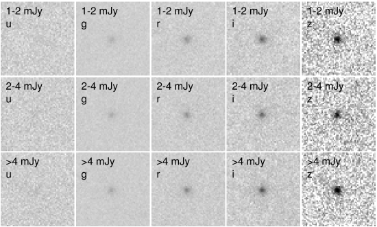
Figure 6: The stacked images of the radio-selected cut-out images, for each radio flux bin and SDSS band. We use the same inverted logarithmic scaling for all images. The width of the images is 24 arcsec.

3.4 Sky level recalibration

The SDSS imaging pipeline (Stoughton et al., 2002) estimates the local sky level using clipped median in 256 by 256 pixel boxes, centred on every 128 pixels of the 2048 by 1489 pixel frames. A sky constructed by interpolation of these local sky estimates is then subtracted from the frames, prior to co-adding the frames of different scans. The resolution of the sky estimation does not allow for complete elimination of the light from high latitude galactic clouds due to their finer texture. Although the imaging pipeline attempts to subtract the wings of the PSF of saturated stars, the algorithm is not too aggressive. Wings of stars can easily fill the $80$ by $80$ arcsec cut-outs entirely. These two effects can significantly increase the average background level and reduce the contrast of the stacked images, thus need to be eliminated.

The cut-outs we generate show a tiny bias of the background level towards negative values. Because we are dealing with objects that are extremely faint in the optical bands (in the range of $30$–$300$ nJy arcsec^-2 or $25$–$28$ mag arcsec^-2), this small bias (estimated to be about $10$–$60$ nJy arcsec^-2 or $27$–$29$ mag arcsec^-2, depending on the photometric filter used) would significantly affect the photometry of the stacked images. The bias is likely to be the consequence of a remaining gradient in the background level in the whole co-added Stripe 82 frames, which becomes apparent if only small parts of the frames are considered. Also, the algorithm applied to co-add the Stripe 82 images has used $2.326\sigma$ clipping to determine the sky level, while we use a much restrictive $1\sigma$ masking threshold. As a consequence, the sky level of the cut-outs has to be re-estimated. To do this, we simply subtract the average value of the unmasked pixels from the cut-outs on a per image basis.

3.5 Selection bias of the stack sky levels

When composing the DCS sample, we imposed selection criteria based on the separation of the radio sources from the neighbouring optical sources. This introduces a strange bias to the background of the cut-outs, as we will show in this section.

To investigate the issue, we generate stacked images of cut-outs centred on random coordinates. We call these special stacks random stacks. First, for every DCS source coordinate pair, a random coordinate pair is generated within the same Stripe 82 frame where the DCS object is. We require these random points to satisfy the same selection criteria as the DCS objects, i.e. they are at least $3$ arcsec away from any optically detected Stripe 82 co-added sources and at least $1.5$ arcmin away from any other FIRST radio sources. Second, random cut-outs are masked as described in Section 3.2. Third, the pixel values are averaged according to the following formula:

$$s^{\textrm{R}}_{kl}=\frac{\sum_{i=1}^{N}p^{\textrm{R}}_{ikl}w_{ikl}}{\sum_{i=1}^{N}w_{ikl}},$$ (2)

where $s^{\textrm{R}}_{kl}$ denotes the pixel value at the $k$ and $l$ pixel coordinates of the random stack image (the upper R is used to identify that this is a random stack); $p^{\textrm{R}}_{ikl}$ is the pixel value of the random cut-outs, where $i$ indexes the individual cut-outs; $w_{ikl}$ is the mask, its value is 0 is the pixel is masked out and 1 if it is not; $N$ is the total number of cut-outs, as before. Separate random stacks are generated for all five SDSS bands and for all three DCS subsamples. (Note, that it is important that the random coordinates are chosen to be within the same Stripe 82 frame as the original DCS source coordinates are, so different random stacks are necessary for each subsample.)

To characterize the variance of the random stacks, we generate 50 of them using different sets of random coordinates. To get the correction term $c_{kl}$ introduced in Section 3.3, we combine the 50 random stacks into a super-stack. The super-stack (denoted as $c_{kl}$ in Eq. 1) is simply the pixel-wise average of the 50 random stacks.

The pixels of these final random super-stacks are once more averaged in annuli centred on the middle of the images to determine the radial surface brightness profile of the background. The resulting profiles are plotted in Fig. 7.

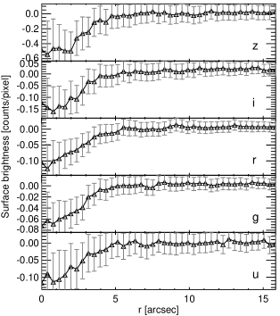
Figure 7: Radial surface brightness profiles of the random super-stacks (the average of 50 random stacks per imaging filter), created for the coordinates of the $1$ – $2$ mJy subsample using $1\sigma$ masking threshold. The letters of the imaging filters are indicated next to the curves. Error bars show the variance of the values in each annulus.

The significant feature of the radial surface brightness profiles are the dark spots at the centres of the images. They are very well visible even though variance is higher at these small radii due to the lower pixel counts. We account these dark spots to the selection criterion that restricts coordinate selection to coordinates that are at least $3$ arcsec away from the centres of the closest Stripe 82 objects. The plateaus of the surface brightness profiles of the random stacks come from the faint light of nearby objects. Contribution to these plateaus from stray light from farther bright objects is also expected.

4 The reliability of the stacking method

Simple averaging is known to be sensitive to outliers, thus reliable masking of the bright pixels of cut-outs prior to averaging is inevitable. We apply three tests to confirm the robustness of our masking and stacking method: a) jackknife analysis of the entire stacking process, b) analysis of the dependence of the magnitude of the central peaks on the masking threshold, c) analysis of the dependence of the pixel value histogram of the stacked images on the masking threshold.

4.1 Jackknife analysis

To estimate the error introduced by possible outliers, we perform a jackknife analysis of the stacking method by repeating the entire processing numerous times, but leaving out a single cut-out image in every iteration.

Fig. 8 shows the relative frequency of the estimated magnitudes of the central peaks for $709$ jackknife runs for the $g$, $r$ and $i$ band images of the $1$ – $2$ mJy radio flux bin. The distributions are slightly biased towards the fainter magnitudes as a result of a few significant outliers. The few objects responsible for the faint-end wing of the distribution affect the stacked flux by approx $1$ per cent, thus they have a flux roughly a factor $8$ larger than the average considering a sample of $709$ objects.

The statistical errors of the magnitudes based on the jackknife analysis turned out to be in the $0.1$–$0.2$ mag range. In Section 5.2, we will use these error estimates to characterize the uncertainties of the photometry.

Figure 8: Distribution of the magnitude of the central peak from the jackknife stacks (histogram). The means of the fitted Gaussians (solid lines) are slightly offset to the right (see text).

4.2 Effect of the masking threshold

Masking is required to eliminate the bright pixels of the cut-outs in order to avoid the contamination of the stacked images from moderately bright, but still detectable images – we are only interested in the undetected, faint objects. In Section 3.2.2, a masking threshold was introduced. The masking threshold is determined from the pixel value distribution of the co-added images by multiplying the variance of the pixel values with a well-chosen number. Here we show that setting the threshold at $1\sigma$ is a good choice.

Fig. 9 shows the measured magnitudes of the peaks detected in the centres of the stacked images for each SDSS band and radio luminosity bin as a function of the masking threshold. It is observable that the initially increasing curves reach a plateau around $1\sigma$ and then start to decrease slowly. The explanation is simple: If the masking threshold is too low, we lose many pixels belonging the the investigated faint objects. On the other hand, if the threshold is too high the background level of the image is increased by the pixels belonging to other, nearby objects causing the contrast of the stacked images to be lower and the measured magnitudes to be fainter. The maxima of most of these curves are usually located in the $0.75\sigma$ – $1.25\sigma$ range, so setting the masking threshold at $1\sigma$ is obvious.

Note that if we were to use a smoothing kernel of a different radius to construct the masks, the start of the plateau of the curves in Fig. 9 would be at different $\sigma$ values. Increasing the radius of the kernel would move the beginning of the plateaus to the left. This behaviour is a direct consequence of the masking process; a mask created with a larger kernel would let more pixels from nearby faint, point-like objects into the stack at a given masking threshold, because a wide kernel would smooth out these objects to such an extent that their pixel values would become less than the masking threshold. This is why it is important to use a smoothing kernel not much larger in diameter than the size of the faintest identifiable objects of the co-added images. This diameter is roughly the FWHM of the PSF.

4.3 Flux deficit in the central aperture

Because the masks are uniform in the whole cut-out image area, some pixels at the central source location can also be masked. This can introduce a slight flux deficit in the stack because of some marginally detected sources being masked out; ca. $1$ – $5$ per cent of the central pixels are lost, depending on the filter ($u$ is the lowest, $i$ is the highest). If we did not mask in the centre, some contaminating outlier pixels would easily get into the stack, causing a significant bias in the photometry (because we would overestimate the flux of the stacked source). So, this is a necessary trade-off in order to ensure the photometric quality of the stacked images.

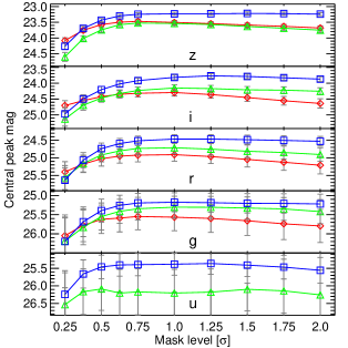
Figure 9: Measured flux of the central peak in the stacked images as a function of masking threshold in units of $\sigma$. The panels show the five SDSS bands, while colours refer to the radio luminosity bins (red diamond: $1$–$2$ mJy, green triangle: $2$–$4$ mJy, blue square: $>4$ mJy).

4.4 Effect of possible outlier pixels

It is important to show that the signal emerging from the centres of the cut-outs after averaging comes from real objects and not just from a few outlier pixels. Cut-out images after masking will contain sky pixels (background), pixels of nearby faint objects that are above the background level, and pixels near the centres of the cut-outs actually belonging to the radio sources of our interest. The pixel values of these later ones are very close to the background noise level. In Fig. 10 (left column), we plot the distribution of pixel values of the $r$-band cut-outs in the $1$–$2$ mJy radio luminosity bin inside and outside of a central circular aperture with a radius of $2$ arcsec for three different values of the masking threshold. The solid lines (shaded areas) show the normalised distributions of the pixel values inside (outside) the central aperture. The panels in the right column show the difference of the distributions: the distributions of the background pixels subtracted from the distributions of the pixels within the apertures centred on the radio objects. There are two important things to observe in Fig. 10: a) the distribution of background pixels have a long tail towards bright pixels, and b) the distribution of the pixels inside the aperture is slightly shifted to the right with respect to the background.

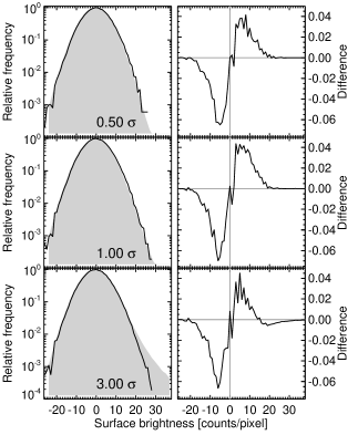
Figure 10: Left column: Distributions of pixel values of the $r$-band cut-outs in the $1$–$2$ mJy radio luminosity bin inside (solid curves) and outside (grey area) of a central circular aperture with a radius of $2$ arcsec for three different values of the masking threshold (indicated in each panel). Panels in the right column show the difference of the two distributions: the distributions of the background pixels subtracted from the distributions of the pixels within the apertures centred on the radio objects.

The long tail of the distribution of background pixels comes from the relatively bright pixels of nearby faint objects, like the unmasked diffuse envelopes of nearby galaxies. The central aperture does not contain such pixels because of the selection criterion we used to select only those radio sources which are separated from the nearest optically detected objects by at least $3$ arcsec.

The small shift between the peaks of the distributions is due to the actual signal we are looking for. Optical emission from the radio objects is so faint that the individual pixels cannot be distinguished from the noise of the background, but stacking the cut-outs reveals the signal.

The lack of the bright tail of the pixel value distribution of the central pixels and the small shift between the distributions of background pixels and central pixels confirm our claim that the detected peaks in the stacked images come from numerous faint objects and not from just a few brighter (but still faint) outlier objects.

5 Results

Altogether 15 stacked images were created, one for each SDSS filter and for each DCS subsample. In Fig. 6 we have already plotted the images of the stacks. The PSF-like point sources are clearly visible at the centres, and we consider them to be the optical signal coming from the FIRST radio sources. The peaks show a monotonically increasing intensity towards the longer wavelength bands, that is the sources are red in the optical colours.

5.1 Signal-to-noise ratios

The signal-to-noise ratios and rms background noise levels of the stacks are summarized in Table 3. These signal-to-noise ratios are sufficient to calculate the photometric properties of the central peaks, except for the $u$ filter.

	S/N ratio						rms noise
Filter	$S_{\text{int},1400}$ bin [mJy]						$\left[\text{mag}~{}\text{arcsec}^{-2}\right]$
	$1-2$		$2-4$		$>4$
$u$	0.	6	1.	1	1.	7	29.	0
$g$	5.	7	6.	1	7.	4	30.	0
$r$	6.	9	7.	4	9.	0	29.	5
$i$	8.	5	8.	7	10.	8	29.	0
$z$	5.	9	5.	5	7.	4	27.	6

Table 3: Signal-to-noise ratios and rms background noise levels of the stacked images.

5.2 Photometry

The SDSS catalogue uses a special magnitude system designed for noisy imaging (Lupton et al., 1999). The definition of the so-called ‘luptitudes’ is based on the $asinh$ function instead of the traditionally used logarithm, and it contains the scaling constant $b$. This constant was calibrated for typical SDSS frames with objects of average brightness. When determining the magnitudes of the central peaks of the stacks, it would be appropriate to use the same magnitude system as SDSS. In our case, however, the value of $b$ had to be recalibrated to account for extremely faint objects, which would mean the recalibration of the whole SDSS magnitude system as well. For this reason, we decided to use the conventional Pogson magnitudes instead.

Because the co-added Stripe 82 images are sky-substracted, calibrated for atmospheric extinction and remapped to a common zeropoint, the transformation of counts into magnitudes is straightforward:

$$\text{mag}_{\lambda}=-2.5\log_{10}\text{counts}+30-A_{\lambda}$$ (3)

where $A_{\lambda}$ is the correction for the galactic extinction, discussed later in Section 5.3.

We measure the brightness of the central peaks in a circular aperture with a radius of $5$ arcsec. The size of the aperture was chosen to be slightly larger than the double of FWHM of the central peaks ($1.5$ – $2$ arcsec, depending on the band). To characterize the photometric uncertainties, we use the standard deviations provided by the jackknife stacks.

5.3 Estimating the galactic extinction

We correct for the galactic extinction after stacking. We could have applied an intensity rescale to each cut-out image prior stacking, but that would have altered the noise characteristics of the images. Instead, we correct for galactic extinction using an average value of $E(B-V)$. The average extinction is calculated from values of the extinction in the directions of the DCS source coordinates. The values of $E(B-V)$ are taken from Schlegel et al. (1998). Table 4 summarizes the value of the galactic extinction and the correction magnitudes for every imaging filter. The average value of $E(B-V)$ is equal for all three subsamples to two decimals. Note, however, that the scatter in extinction values is almost as large as the average extinction itself. Still, this only introduces a small error in the final colour index estimates, as we show below.

$\left<E(B-V)\right>$	$\sigma_{E(B-V)}$
0.048	0.025

$A_{u}$	$A_{g}$	$A_{r}$	$A_{i}$	$A_{z}$
0.25	0.18	0.13	0.10	0.07

Table 4: Average and standard deviation of the $E(B-V)$ values of the DCS sample, with the correction magnitudes.

5.4 Optical magnitudes

The optical magnitudes of the central peaks are summarized in Table 5 for every SDSS filter and DCS subsample. The quoted magnitudes are already corrected for average foreground extinction, as explained in Section 5.3.

Filter	$S_{\text{int},1400}$ bin [mJy]
	$1-2$				$2-4$				$>4$
$u$	27.	21 $\pm$	2.	63∗	26.	20 $\pm$	0.	55	25.	38 $\pm$	0.	38
$g$	25.	57 $\pm$	0.	16	25.	31 $\pm$	0.	13	25.	18 $\pm$	0.	12
$r$	24.	91 $\pm$	0.	19	24.	71 $\pm$	0.	12	24.	47 $\pm$	0.	09
$i$	24.	29 $\pm$	0.	13	24.	15 $\pm$	0.	12	23.	82 $\pm$	0.	09
$z$	23.	50 $\pm$	0.	15	23.	54 $\pm$	0.	16	23.	23 $\pm$	0.	12

Table 5: Optical magnitudes of the central peaks identified in the stacked images for every DCS subsample. The photometric calibration is described in Section 5.2. Values are corrected for average foreground galactic extinction. * Aperture radius: $3$ arcsec.

According to these results, the average optical magnitudes of the central peaks are about $1$ mag fainter than the practical detection limit of the Stripe 82 co-added catalogue. There is a slight increase in optical brightness in all optical wavelength bands towards higher radio fluxes. The error of the photometry strongly depends on the imaging filter; the noise becomes really significant in the ultraviolet.

5.5 Radial profiles

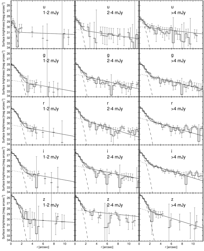
Figure 11: Surface brightness profiles of the stacked images around the central peaks. The graphs in each column show the profiles for a given radio flux bin for all five SDSS imaging filters. Solid lines indicate the model fits; dashed lines are the Gaussian components; dotted lines are the exponential components. Error bars represent the variance of the values in each annulus.

To determine the radial profiles of the stacked objects, we first determine the exact centres of the central peaks in the images by fitting two-dimensional Gaussians to the pixel values. Then we average the pixels in annuli of $\text{d}r=0.4$ arcsec centred on the fitted positions of the peaks.

In Fig. 11 we plot the radial profiles of the background corrected stacks for every filter and DCS subsample. The central peaks of the profiles are clearly visible, just like the faint, extended components that decrease with radius.

We fit the profiles with the combination of a Gaussian and an exponential function. These fits are also displayed in Fig. 11 (solid lines). The fitting function is formulated the following way:

$$I(r)=\frac{A}{\sqrt{2\pi}\,\sigma}\exp{\left(-\frac{r^{2}}{2\sigma^{2}}\right)}+B\,\exp{\left(-\frac{r}{r_{0}}\right)}$$ (4)

The fitting is done in two phases. First, we fit the outer part ($3<r<8$ arcsec) of the profiles with the exponential term to obtain the value of $B$ and the scalelength $r_{0}$. Then, the resulting exponential fit is subtracted from the original profile. Finally, the residuals are fitted with Gaussians in the $0$–$5$ arcsec radius range. The fitted parameters are summarized in Table 6. The central PSF-like peaks cut off around $r\simeq 2$ – $3$ arcsec, but the exponential component is traceable to ca. $r\simeq 15$ arcsec. The $u$ profiles in the $1$–$2$ mJy and $>4$ mJy bins do not have good enough data quality to really trust the fitted values.

		$S_{int,1400}$ [mJy]
		$1-2$				$2-4$				$>4$
$u$	$A$	9.	56 $\pm$	5.	90	19.	96 $\pm$	4.	92	21.	62 $\pm$	3.	20
	$\sigma$	0.	51 $\pm$	0.	32	0.	62 $\pm$	0.	16	0.	63 $\pm$	0.	10
	$B$	1.	57 $\pm$	0.	82	2.	55 $\pm$	1.	59	3.	97 $\pm$	2.	23
	$r_{0}$	28.	70 $\pm$	56.	13	7.	24 $\pm$	5.	41	9.	38 $\pm$	9.	09
$g$	$A$	44.	23 $\pm$	2.	47	39.	59 $\pm$	2.	79	46.	26 $\pm$	2.	82
	$\sigma$	0.	87 $\pm$	0.	05	0.	68 $\pm$	0.	05	0.	75 $\pm$	0.	05
	$B$	1.	59 $\pm$	0.	90	4.	47 $\pm$	1.	46	4.	61 $\pm$	1.	26
	$r_{0}$	6.	01 $\pm$	4.	14	4.	63 $\pm$	1.	36	4.	54 $\pm$	1.	11
$r$	$A$	87.	24 $\pm$	2.	78	63.	10 $\pm$	3.	84	87.	39 $\pm$	4.	56
	$\sigma$	0.	82 $\pm$	0.	03	0.	62 $\pm$	0.	04	0.	72 $\pm$	0.	04
	$B$	2.	82 $\pm$	1.	04	10.	00 $\pm$	3.	41	9.	16 $\pm$	2.	05
	$r_{0}$	5.	98 $\pm$	2.	82	3.	52 $\pm$	0.	89	3.	85 $\pm$	0.	67
$i$	$A$	173.	73 $\pm$	6.	60	139.	96 $\pm$	7.	76	147.	14 $\pm$	8.	10
	$\sigma$	0.	82 $\pm$	0.	03	0.	72 $\pm$	0.	04	0.	67 $\pm$	0.	04
	$B$	4.	39 $\pm$	2.	13	9.	71 $\pm$	3.	04	20.	09 $\pm$	3.	47
	$r_{0}$	6.	03 $\pm$	3.	94	5.	34 $\pm$	1.	68	3.	55 $\pm$	0.	44
$z$	$A$	394.	57 $\pm$	26.	77	279.	43 $\pm$	27.	24	405.	69 $\pm$	20.	20
	$\sigma$	0.	74 $\pm$	0.	05	0.	62 $\pm$	0.	06	0.	71 $\pm$	0.	04
	$B$	4.	27 $\pm$	2.	13	18.	69 $\pm$	8.	40	25.	27 $\pm$	11.	34
	$r_{0}$	18.	12 $\pm$	36.	27	10.	37 $\pm$	8.	10	3.	48 $\pm$	1.	31

Table 6: Fitted parameters of the radial profiles: $A$ [nJy arcsec^-1], $\sigma$ [arcsec], $B$ [nJy arcsec^-2], $r_{0}$ [arcsec].

5.6 Possible origins of the exponential component

The existence of an exponentially decreasing component of the radial profiles is obvious from Fig. 11. The value of the scale parameter $r_{0}$ are listed in Table 6. Excluding the low quality fits of the $u$ filter, the value of $r_{0}$ is consistently around $r_{0}\simeq 3.5$ – $5.5$ arcsec.

It is very important to consider that the PSF of SDSS images already shows an extended component. To investigate the contribution of these extended wings to the radial profiles of our stacks, we applied our stacking algorithm to images of faint stars. The stacks of stars showed a similar exponential tail with a scale parameter $r_{0}$ in the range of $2$ – $3$ arcsec, depending on the photometric band. These values are significantly smaller than the scale lengths derived from the stacks of our radio-selected objects. The radial profiles of our stacks clearly show an excess over the stellar PSF at the tails. For more discussion on the effect of the PSF wings on the radial profiles of stacked objects, see Zibetti et al. (2004) and de Jong (2008).

It is very risky to draw any conclusions from the observation of the exponential component, especially in the absence of information about the redshift of the radio-selected objects. Because the redshifts are unknown, we cannot rescale our sources to the same physical scale before the stacking. The physical scales could therefore be very different between the objects that are stacked together.

However, it is interesting to see what the measured angular scalelength translates to at different redshifts. If we make the assumption that the majority of the DCS sample lies around $z\simeq 0.1$, the corresponding scalelength is $6$-$10$ kpc. At $z\simeq 1$, the scalelength would be $28$-$45$ kpc. The former range is consistent with the size of individual galaxies, which might suggest that we see the host galaxies of the quasars. The latter scalelength could correspond to the diameter of merging systems. It can also be imagined that the excess in surface brightness at large radii comes from undetected galaxies clustered around the radio sources.

5.7 Spectral energy distributions

One important finding is that the stacked objects have unusually red average colours, as listed in Table 7. The colour indices seem to be independent from the apparent radio luminosity. In Fig. 12, we plot the SEDs of the central peaks of the stacked images for all three DCS subsamples (solid lines with symbols). The optical spectral indices ($\alpha_{\nu}$) are determined by fitting power-law functions to the fluxes, and the results are listed in Table 8.

Because the redshift distribution of the DCS sample is unknown, the colours of the stacked object might not correctly represent the average spectral slope of the sample. In order to obtain the correct colours, one should perform k-correction for each DCS source individually – obviously, this cannot be done in this study. However, if we assume that the majority of the sources have a power-law SED in the optical and ultraviolet regime, with similar spectral slopes, the k-correction magnitudes in this case are independent of wavelength, and hence the colour indices remain unchanged.

However, we note that if the objects had a redshift distribution similar to that of the LBDS sample mentioned in Section 1.3 (Waddington et al., 2001), that is, the majority of the objects had $z<1.5$, based on the average spectral index of $\alpha_{\nu}=-2.5$, then the average k-correction would be $\sim 0.9$ mag in every band.

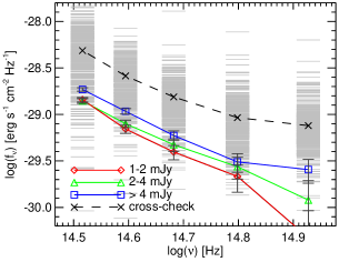
Figure 12: Optical SEDs (symbols connected with solid lines) of the central peaks identified in the stacked images for every DCS subsample. The short grey lines indicate the fluxes of the individual objects of the cross-check sample described in Section 6. The dashed line is the average SED of the cross-check sample.

Filter	$S_{\text{int},1400}$ [mJy]
	$1-2$				$2-4$				$>4$
$g-r$	0.	7 $\pm$	0.	2	0.	6 $\pm$	0.	2	0.	7 $\pm$	0.	1
$r-i$	0.	6 $\pm$	0.	2	0.	6 $\pm$	0.	2	0.	6 $\pm$	0.	1
$i-z$	0.	8 $\pm$	0.	2	0.	6 $\pm$	0.	2	0.	6 $\pm$	0.	1

Table 7: Optical colour indices of the central peaks identified in the stacked images for every DCS subsample.

$S_{\text{int},1400}$	$\alpha_{\nu}$
bin [mJy]
$1-2$	$-2.9\pm 0.3$
$2-4$	$-2.5\pm 0.1$
$>4$	$-2.2\pm 0.3$

Table 8: Average spectral indices of the central peaks.

Vanden Berk et al. (2001) calculated composite spectra of more than 2200 SDSS quasars and they found $\alpha_{\nu}=-0.44$ for the spectral continuum. Ivezić et al. (2002) determined spectral indices individually for 6868 quasar spectra with a mean of $\alpha_{\nu}=-0.45$. The bulk of their distribution is in the range of $-1<\alpha_{\nu}<0.2$. Gregg et al. (2002) suggested $\alpha_{\nu}<-1$ as a definition of a red quasar. They found two sources with $\alpha_{\nu}\approx-3.7$ and $\alpha_{\nu}\lesssim-4.6$, which they called extraordinarily red. Richards et al. (2006) defined Type 1 quasars by $\alpha=-0.5\pm 0.3$ and reddened Type 1 quasars by $\alpha_{\nu}<-1$, which both have broad emission lines. The values for our stacked sources are in the range $-2.9\leq\alpha_{\nu}\leq-2.2$. However, note that we cannot account for the effect of emission lines when calculating the spectral indices, and therefore we have $\alpha_{\nu}$ values from fitting of the entire spectrum (continuum and lines). Measurements of $\alpha$ by others usually based on the spectral continuum only.

If we account the red colours to intrinsic extinction, the values of $-2.9\leq\alpha_{\nu}\leq-2.2$ require unusually high column densities of the obscuring dust. The absolute value of the spectral index becomes slightly smaller with increasing radio flux. This might suggest – if we assume that the redshift distribution of the objects is narrow, or at least similar for all radio flux bins – that the brighter radio sources are slightly less reddened on average.

6 Discussion

Because the individual objects of the DCS sample are undetectable in the optical images, we can only discuss the average optical properties of the objects based on their stacked images. We hope that these average values represent the original distribution of the sources well. With the lack of direct detections, the homogeneity of the sample cannot be proven. However, it is still worth comparing the DCS sample with samples of very similar selection criteria, except that the radio-selected objects are also detected in the optical.

6.1 Construction of the cross-check sample

In order to compare the average optical properties of the DCS objects to better-known objects, we construct a cross-check sample of radio selected sources, but in this case with identified optical counterparts. We select FIRST radio point sources that have optical counterparts within $1.5$ arcsec in the Stripe 82 catalogue, but not in the singly observed (thus less faint) SDSS Data Release 6 (DR6) catalogue within $3$ arcsec. The 1.5-arcsec matching radius was chosen in accordance with Ivezić et al. (2002), who matched FIRST with SDSS using the same separation limit. Based on their study, we expect similar completeness ($\sim 85$ per cent), and a slightly higher level of contamination than their $3$ per cent, because the larger source density in the Stripe 82 co-added catalogue increases the false-positive match rate. All other selection criteria for the FIRST sources are the same as described in Section 2.

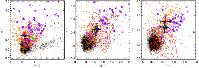
Figure 13: Colour-colour diagrams of the stacked objects (filled circles – red: $1$–$2$ mJy, green: $2$–$4$ mJy, blue: $>4$ mJy), the cross-check sample (orange crosses), normal Type 1 quasars (black dots), red Type 1s (purple squares), and Type 2s (red contour lines). See the description of the samples in Section 6.2. A colour version of this plot is available on-line.

Because the co-added Stripe 82 is a significantly deeper survey than the singly observed SDSS DR6, we expect to find objects that are too faint to be detected in DR6 but are visible in the co-added Stripe 82 images. Indeed, $1349$ FIRST sources were found with optical magnitudes in the range $24\geq m_{i}\geq 22$ mag. We apply further restrictions on the photometric quality of the cross-check sample (i.e. the error in $u$ and $g$ model magnitudes must be less than $0.8$ and $0.5$ mag, respectively). The final sample consists of $394$ co-added Stripe 82 sources, which are optical counterparts of isolated, compact FIRST radio sources with integrated luminosities larger than $S_{\text{int},1400}\geq 1$ mJy.

We have published a catalogue on the multiwavelength photometric properties of the cross-check objects, compiled from the Stripe 82 co-added survey (optical), the FIRST survey (radio) and two infrared surveys: the United Kingdom Infrared Telescope (UKIRT) Infrared Deep Sky Survey (UKIDSS) and the Wide-field Infrared Survey Explorer (WISE). The infrared cross-identification is described in Section 6.3. The catalogue is available on-line at http://www.vo.elte.hu/doublestacking.

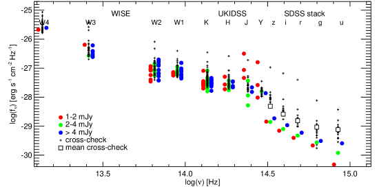
Figure 14: Optical and infrared SEDs of the DCS sample (coloured dots: red: $1$ – $2$ mJy, green: $2$ – $4$ mJy, blue: $>4$ mJy subsamples) and the cross-check sample (black crosses). The data points in all infrared bands are individual detections, while the optical fluxes of the stacked objects are average values. We plot only those objects of the cross-check sample that have matching detections in the $K$ band. The average optical fluxes of the entire cross-check sample are plotted with black squares. (A colour version of this figure is available on-line.)

We plot the optical fluxes of the cross-check sample in Fig. 12 as grey dashes. The average fluxes of the cross-check sample (crosses connected with a dashed line) and the fluxes of the stacked objects (points connected with solid lines) are also plotted in the same plot. The average magnitudes calculated from the stacked images are about $1.2$–$1.6$ mag fainter than those of the cross-check sample, but the slopes of the SEDs are similar.

6.2 Comparison with the cross-check sample and optically detected quasars

To evaluate the average optical properties of the DCS objects we compare them to three samples of quasars. The first sample is the fifth edition of the SDSS quasar catalogue containing 105783 objects (Schneider et al., 2010). The catalogue is composed of SDSS quasars with luminosities higher than $M_{i}<-22.0$, having at least one emission line with FWHM higher than $1000~{}{\text{km}}~{}{\text{s}}^{-1}$ or showing interesting/complex absorption features. The quasar redshifts range from $0.065$ to $5.46$, with a median value of $1.49$. The majority of the sample can be classified as normal (unreddened) Type 1 quasars. The second quasar sample consists of 51 red Type 1 quasars (Urrutia et al., 2009). Urrutia et al. matched the FIRST-2MASS red quasar survey (Glikman et al., 2007) with SDSS, and compiled this sample of spectroscopically confirmed red Type 1 quasars. The third sample contains 887 spectroscopically confirmed Type 2 quasars from SDSS with redshifts $z<0.83$ (Reyes et al., 2008). The stacked objects are about $1.4$ mag fainter in the $i$ band than the average of the cross-check sample and the latter is $3$ mag fainter than the red Type 1 sample.

In Fig. 13 we plot the optical colour-colour diagrams of the stacked objects, the cross-check sample and the three quasar samples. It is clear that on average our DCS sample is significantly redder than normal Type 1 quasars. The $r-i$ and $i-z$ colours suggest that the DCS sample is more likely to consist of reddened Type 1s than Type 2s.

6.3 Infrared counterparts

If we accept the assumption that our radio sources are AGNs heavily obscured by dust surrounding the central regions, it is straightforward to look for excess in their infrared emission. For this reason, we looked for infrared counterparts to the DCS sample in the extragalactic near-infrared UKIDSS Large Area Survey (LAS) DR7 catalogue (Dye et al., 2006) and in the WISE preliminary release mid-infrared source catalogue (Wright et al., 2010). Within the sky regions overlapping with SDSS Stripe 82, about $4$ per cent of the radio sources ($72$ objects) were detected by the UKIDDS in any of the infrared bands, using a matching radius of $1.5$ arcsec. Only a few dozen objects have matching counterparts in the WISE catalogue in at least one band. This detection rate is about $5$ per cent. The infrared magnitudes are close to the detection limits of both surveys and the scatter of the magnitudes is small. This means that only the very bright end of the sample is detected in infrared.

The cross-check sample has a much higher detection rate, with $123$ sources detected in the near-infrared ($37$ per cent) and $33$ in the mid-infrared ($32$ per cent). The distribution of the infrared magnitudes is similar to that of the DCS sample, with cut-off at the faint end because of the magnitude limit. In Fig. 14, we plot the optical to mid-infrared SED of our samples: the individually detected objects of the DCS sample (colour dots) and the cross-check sample (black crosses). The data points in all infrared bands are individual detections, while the optical fluxes of the stacked objects are average values for the three DCS subsamples. We plot the average optical fluxes of the cross-check sample with black squares.

The cross-check sample has an average SED with a slope of $\alpha_{\nu}\simeq-2.0$ (see Fig. 12), less steep than the slope of the average optical SED of the DCS sample. Exact physical interpretation is difficult, however, as we do not have information on the composition of the samples. If we assume that the objects in the samples are intrinsically similar, the gradual steepening of the spectral slopes with decreasing optical brightness can be attributed to obscuration by dust.

Glikman et al. (2004) constructed a sample of bright near-infrared sources that are detected at radio wavelengths but unidentified on the Palomar Observatory Sky Survey (POSS) plates, with the aim of finding dust-obscured quasars. They have defined a region in the $R-K$, $J-K$ colour plane, in which $50$ per cent of the radio-selected objects are highly reddened quasars ($J-K>1.7$ and $R-K>4$). To compare our samples to these criteria, we converted SDSS magnitudes to Johnson $R$ using the equations of Jester et al. (2005). There are $17$ sources of our cross-check sample that have detections in both $J$ and $K$ infrared bands. For objects not detected in the $J$ band (the majority), we assume a lower limit of the $J-K$ colour index using the limiting magnitude of the survey. In Fig. 15, we plot the cross-check objects in the $R-K$, $J-K$ colour plane. Only a few objects have valid $J$ magnitudes (diamonds); object with lower limits in $J$ are plotted with grey arrows. The majority of our sources ($77$ per cent) are in the red quasar region of the plane.

Only a few objects of the DCS sample were detected in infrared individually. It is very likely that the optical flux distribution of these objects differs significantly from the distribution of the entire DCS sample. Because the DCS sources are undetected in the optical, we can easily determine an upper limit on their $R$ fluxes; they should be fainter than the Stripe 82 co-added survey limit ($R\gtrsim 24.2$).

Therefore, we are able to estimate a lower limit on the $R-K$ colour of the DCS sources with infrared detections. We also calculate a lower limit on $J-K$ in the absence of reliable $J$ band fluxes. The results are plotted in Fig. 15 with coloured symbols (arrows), one for each DCS subsample. It is apparent that the $R-K$ values are in the red quasar region, even if we assume brighter $R$ fluxes. The $J-K$ colours are also in that region, but much closer to the border.

It is hard to estimate the possible fraction of red quasars in our samples based on the available infrared data. As for the cross-check sample, with a $34$ per cent detection rate and with at least $77$ per cent of the infrared-matched objects lying in the red quasar region of the $R-K$, $J-K$ plane, we find that at least $13$ per cent of all objects are undoubtedly dust-obscured quasars. However, this is a weak lower limit on their number, because we only see the brightest infrared counterparts as a result of the relatively high infrared flux limit of the observations.

7 Summary

We have presented an analysis based on an image stacking technique, to reveal the visible wavelength light from the unresolved sources of the FIRST radio survey that remain undetected in the SDSS Stripe 82 co-added catalogue. The sample consists of 2116 objects, which have been divided into three subsamples according to the radio flux. We stacked cut-out images centred on the object coordinates from the SDSS Stripe 82 co-added survey. The main results of our study are as follows.

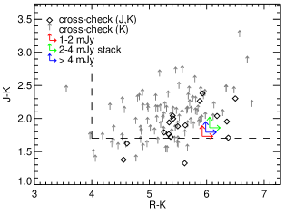
Figure 15: Colour indices of the cross-check sample and the DCS sample in the $R-K$;$J-K$ plane. Diamonds denote cross-check sample objects with valid $J$ band data, arrows denote cross-check objects with the $J$ band lower limit only and coloured arrows denote stacked objects (red: $1$ – $2$ mJy, green: $2$ – $4$ mJy, blue: $>4$ mJy subsamples). The arrows mark the lower limits on $R-K$ and $J-K$. The dashed lines bound the upper right region, where $50$ per cent of the sources are red quasars, according to Glikman et al. (2004).

1. We have presented an image stacking algorithm with an efficient masking technique to reveal the average optical emission of 2116 optically undetected sources (DCS sample) selected based on the VLA FIRST radio survey.

2. We have detected the average optical emission of these radio sources (with $26.6$ mag $5\sigma$ detection limit in $r$ band), and we have calculated the $ugriz$ magnitudes of the peaks apparent in the centres of the stacked images (see Table 5). The colours of these peaks imply a steep, red optical spectrum with spectral indices of $-2.9\leq\alpha_{\nu}\leq-2.2$.

3. The average surface brightness profiles of the stacked objects show Gaussian peaks in the centres, which continue in outwards fading exponential components traceable to $\sim 15$ arcsec. The surface brightness of these components peaks at approximately $2$–$3$ mag arcsec^-2 fainter than the peak surface brightness of the central point-like components.

4. We have created a radio-selected sample with faint optical detections in the SDSS Stripe 82 catalogue (cross-check sample), similar to the DCS sample. We have identified infrared counterparts to the cross-check objects from the UKIDSS near-infrared and WISE mid-infrared source catalogue (with $37$ per cent detection rate), and we have composed a catalogue of the optical, infrared and radio properties of the sample.

5. We have compared the optical colour indices of the radio-selected and cross-check objects with various spectroscopically identified quasar samples. We have concluded that the distribution of the colours are similar to that of dust-reddened Type 1 quasars, although there is large scatter in the data.

6. We have identified the infrared counterparts of the DCS sources with a $5$ per cent detection rate. We have investigated the distribution of the cross-check and DCS sources in the $R-K$, $J-K$ colour plane, and we have found that the majority of the objects lie in a region where $\sim 50$ per cent of the sources are red quasars.

7. Consequently, the sources of the DCS sample and the cross-check sample are very good red quasar candidates, suitable for future deeper observations and quasar studies. We assume that the forthcoming optical and infrared survey telescopes, such as the Large Synoptic Survey Telescope (LSST) and the James Webb Space Telescope (JWST), might discover many more obscured quasars than previously expected.

References

- Abazajian et al. (2009) Abazajian, K. N., et al. 2009, ApJS, 182, 543
- Antonucci (1993) Antonucci, R. 1993, ARA&A, 31, 473
- Becker et al. (1995) Becker, R. H., White, R. L., & Helfand, D. J. 1995, ApJ, 450, 559
- Becker et al. (2000) Becker, R. H., White, R. L., Gregg, M. D., et al. 2000, ApJ, 538, 72
- Bergvall et al. (2010) Bergvall, N., Zackrisson, E., & Caldwell, B. 2010, MNRAS, 405, 2697
- Casali et al. (2007) Casali, M., Adamson, A., Alves de Oliveira, C., et al. 2007, A&A, 467, 777
- Cutri et al. (2001) Cutri, R. M., Nelson, B. O., Kirkpatrick, J. D., Huchra, J. P., & Smith, P. S. 2001, The New Era of Wide Field Astronomy, 232, 78
- de Jong (2008) de Jong, R. S. 2008, MNRAS, 388, 1521
- Dye et al. (2006) Dye, S., Warren, S. J., Hambly, N. C., et al. 2006, MNRAS, 372, 1227
- Glikman et al. (2004) Glikman, E., Gregg, M. D., Lacy, M., et al. 2004, ApJ, 607, 60
- Glikman et al. (2007) Glikman, E., Helfand, D. J., White, R. L., Becker, R. H., Gregg, M. D., & Lacy, M. 2007, ApJ, 667, 673
- Gregg et al. (2002) Gregg, M. D., Lacy, M., White, R. L., et al. 2002, ApJ, 564, 133
- Gunn et al. (1998) Gunn, J. E., Carr, M., Rockosi, C., et al. 1998, AJ, 116, 3040
- Hall et al. (2002) Hall, P. B., Anderson, S. F., Strauss, M. A., et al. 2002, ApJS, 141, 267
- Hambly et al. (2008) Hambly, N. C., Collins, R. S., Cross, N. J. G., et al. 2008, MNRAS, 384, 637
- Hathi et al. (2008) Hathi, N. P., Jansen, R. A., Windhorst, R. A., Cohen, S. H., Keel, W. C., Corbin, M. R., & Ryan, R. E., Jr. 2008, AJ, 135, 156
- Hazard et al. (1984) Hazard, C., Morton, D. C., Terlevich, R., & McMahon, R. 1984, ApJ, 282, 33
- Helfand et al. (1999) Helfand, D. J., Schnee, S., Becker, R. H., White, R. L., & McMahon, R. G. 1999, AJ, 117, 1568
- Hewett et al. (2006) Hewett, P. C., Warren, S. J., Leggett, S. K., & Hodgkin, S. T. 2006, MNRAS, 367, 454
- Hodge et al. (2008) Hodge, J. A., Becker, R. H., White, R. L., & de Vries, W. H. 2008, AJ, 136, 1097
- Hodge et al. (2009) Hodge, J. A., Zeimann, G. R., Becker, R. H., & White, R. L. 2009, AJ, 138, 900
- Hodge et al. (2011) Hodge, J. A., Becker, R. H., White, R. L., Richards, G. T., & Zeimann, G. R. 2011, AJ, 142, 3
- Hodgkin et al. (2009) Hodgkin, S. T., Irwin, M. J., Hewett, P. C., & Warren, S. J. 2009, MNRAS, 394, 675
- Hopkins et al. (2000) Hopkins, A., Windhorst, R., Cram, L., & Ekers, R. 2000, Experimental Astronomy, 10, 419
- Hopkins et al. (2005) Hopkins, P. F., Hernquist, L., Martini, P., Cox, T. J., Robertson, B., Di Matteo, T., & Springel, V. 2005, ApJ, 625, L71
- Ivezić et al. (2002) Ivezić, Ž., et al. 2002, AJ, 124, 2364
- Jester et al. (2005) Jester, S., Schneider, D. P., Richards, G. T., et al. 2005, AJ, 130, 873
- Lawrence et al. (2007) Lawrence, A., Warren, S. J., Almaini, O., et al. 2007, MNRAS, 379, 1599
- Lupton et al. (1999) Lupton, R. H., Gunn, J. E., & Szalay, A. S. 1999, AJ, 118, 1406
- Manchester et al. (2005) Manchester, R. N., Hobbs, G. B., Teoh, A., & Hobbs, M. 2005, AJ, 129, 1993
- Martínez-Sansigre et al. (2005) Martínez-Sansigre, A., Rawlings, S., Lacy, M., et al. 2005, Nature, 436, 666
- McMahon et al. (2002) McMahon, R. G., White, R. L., Helfand, D. J., & Becker, R. H. 2002, ApJS, 143, 1
- Ogle et al. (1999) Ogle, P. M., Cohen, M. H., Miller, J. S., et al. 1999, ApJS, 125, 1
- Reyes et al. (2008) Reyes, R., et al. 2008, AJ, 136, 2373
- Richards et al. (2003) Richards, G. T., et al. 2003, AJ, 126, 1131
- Richards et al. (2006) Richards, G. T., et al. 2006, ApJS, 166, 470
- Sanders et al. (1988) Sanders, D. B., Soifer, B. T., Elias, J. H., Madore, B. F., Matthews, K., Neugebauer, G., & Scoville, N. Z. 1988, ApJ, 325, 74
- Schlegel et al. (1998) Schlegel, D. J., Finkbeiner, D. P., & Davis, M. 1998, ApJ, 500, 525
- Schmidt & Hines (1999) Schmidt, G. D., & Hines, D. C. 1999, ApJ, 512, 125
- Schneider et al. (2010) Schneider, D. P., Richards, G. T., Hall, P. B., et al. 2010, AJ, 139, 2360
- Skrutskie et al. (2006) Skrutskie, M. F., Cutri, R. M., Stiening, R., et al. 2006, AJ, 131, 1163
- Sprayberry & Foltz (1992) Sprayberry, D., & Foltz, C. B. 1992, ApJ, 390, 39
- Stoughton et al. (2002) Stoughton, C., Lupton, R. H., Bernardi, M., et al. 2002, AJ, 123, 485
- Tal & van Dokkum (2011) Tal, T., & van Dokkum, P. 2011, arXiv:1102.4330
- Trump et al. (2006) Trump, J. R., Hall, P. B., Reichard, T. A., et al. 2006, ApJS, 165, 1
- Urrutia et al. (2009) Urrutia, T., Becker, R. H., White, R. L., Glikman, E., Lacy, M., Hodge, J., & Gregg, M. D. 2009, ApJ, 698, 1095
- Urry & Padovani (1995) Urry, C. M., & Padovani, P. 1995, PASP, 107, 803
- Vanden Berk et al. (2001) Vanden Berk, D. E., et al. 2001, AJ, 122, 549
- Waddington et al. (2001) Waddington, I., Dunlop, J. S., Peacock, J. A., & Windhorst, R. A. 2001, MNRAS, 328, 882
- Webster et al. (1995) Webster, R. L., Francis, P. J., Petersont, B. A., Drinkwater, M. J., & Masci, F. J. 1995, Nature, 375, 469
- Weymann et al. (1991) Weymann, R. J., Morris, S. L., Foltz, C. B., & Hewett, P. C. 1991, ApJ, 373, 23
- Windhorst et al. (1985) Windhorst, R. A., Miley, G. K., Owen, F. N., Kron, R. G., & Koo, D. C. 1985, ApJ, 289, 494
- White et al. (1997) White, R. L., Becker, R. H., Helfand, D. J., & Gregg, M. D. 1997, ApJ, 475, 479
- White et al. (2003) White, R. L., Helfand, D. J., Becker, R. H., et al. 2003, AJ, 126, 706
- White et al. (2007) White, R. L., Helfand, D. J., Becker, R. H., Glikman, E., & de Vries, W. 2007, ApJ, 654, 99
- Wright et al. (2010) Wright, E. L., Eisenhardt, P. R. M., Mainzer, A. K., et al. 2010, AJ, 140, 1868
- York et al. (2000) York, D. G., Adelman, J., Anderson, J. E., Jr., et al. 2000, AJ, 120, 1579
- Zibetti et al. (2004) Zibetti, S., White, S. D. M., & Brinkmann, J. 2004, MNRAS, 347, 556
- Zibetti et al. (2005) Zibetti, S., White, S. D. M., Schneider, D. P., & Brinkmann, J. 2005, MNRAS, 358, 949
- Zibetti et al. (2007) Zibetti, S., Ménard, B., Nestor, D. B., Quider, A. M., Rao, S. M., & Turnshek, D. A. 2007, ApJ, 658, 161