The Fe I 1564.8 nm line
and the distribution of solar magnetic fields

Abstract

The distribution of magnetic field strength at different levels in the quiet solar photosphere was obtained on the basis of the 2D MHD simulation of magnetogranulation and the synthesis of the V profiles of the Fe I $\lambda$ 1564.8 nm line. The shape of the distribution and the position of its maximum vary essentially with depth. The distribution maximum lies, on the average, at 25 mT, but it is found near 35 mT when the spatial averaging of profiles (about $0.5^{\prime\prime}$) is taken into account. The difference between the distributions is due to the errors with which the field strength is determined from V profile splitting. Our analysis reveals that the use of the Fe I $\lambda$ 1564.8 nm line in this method is the most efficient and reliable means of measuring fields above 50 mT, when this line is under the strong-splitting conditions. Under the weak-splitting conditions the measured field strengths are about 20 mT, while under intermediate conditions they are overestimated by 2–4 mT. The field strength distribution obtained with the $\lambda$ 1564.8 nm line in the fields above 50 mT can serve as a standard for testing other techniques and lines. The analysis of the synthesized Fe I $\lambda$ 630.2 nm line profiles supports the conclusion that this line is less suitable for studying field strength distributions because of its weak magnetic sensitivity to fields below 120 mT. In addition, the separation of the $\sigma$-components of this line highly depends on the magnetic vector inclination. The separation of V peaks increases with vector inclination, and this results in a considerable overestimation (by about 20–30 mT) of the strength of weak inclined fields determined by the methods which ignore the Q and U profiles. The derived magnetic field distributions as well as the distributions of asymmetry parameters and V profile zero-crossings are in good agreement with IR polarimetry data. They convincingly confirm the assumption that the structure and strength of photospheric magnetic fields of mixed polarity have continuous spectra down to scales considerably smaller than the resolution threshold. They also suggest that the structure and the scales of magnetic fields are closely related to the granulation structure.

1 Introduction

In our previous studies of the solar magnetogranulation based on 2D MHD simulations by Gadun [3, 5] we have touched upon the very important problem of the distribution of magnetic fields in quiet photospheric regions. As the interest in the weak magnetic fields of the quiet Sun, their nature and structure, and in the interpretation of their observations continues to grow [6, 7, 11], we return to the analysis of the numerical simulation and the synthesis of the Stokes profiles of the infrared line $\lambda$ 1564.8 nm in the context of weak photospheric magnetic fields.

Observations of magnetic fields in the quiet regions on the Sun evidence very weak magnetic fluxes ($10^{-7}$–$10^{-8}$ Wb). The fine field structure cannot be resolved even with the highest spatial resolution, a very high signal-to-noise ratio, and at good seeing. It is also difficult to calibrate correctly the measurements, i.e., to determine the true field strength. For the time being the only possibility to study in detail the small-scale structure of photospheric fields is the direct numerical simulation of magnetoconvection. Our high-resolution studies with a spatial step of 35 km [4, 18] made with the use of 2D MHD magnetogranulation models [3] demonstrated that these models are helpful in understanding various properties of photospheric magnetic fields and their interaction with convective motions on granular scales. These models, when used to study the magnetic field distribution in granules and intergranular lanes, will hopefully provide insight into various problems related to the structure and nature of magnetic fields in the photospheres of the Sun and stars.

Among numerous observation data on the magnetic fields of the quiet Sun, of special interest are the observations of IR lines which turned out to be very helpful in measuring small-scale fields below 0.1 T. The results reveal a complex field structure in quiet regions with low flux densities. The magnetic fields of the quiet Sun seem to be strongly mixed in space – weak, intermediate, and strong fluctuations as well as thin fluxtubes alternate with one another. Theoretical magnetoconvection simulation [2] also suggests that magnetic fields in quiet regions are structurized from the greatest to the smallest ones. Their sizes can be much smaller than the present-day resolution threshold. In addition, the theory as well as observations suggest that the magnetic fields are a mixture of fields of different polarities. Measurements of magnetic fluxes on the quiet Sun outside the supergranulation network [12] indicate that the disbalance of fluxes of different polarities there is smaller than in the network. Recent advances in the observations of weak fields raised the questions as to whether the weak fields are the remnants of a strong magnetic flux circulating at all times due to convection or they are generated by the local dynamo mechanism, whether their dimension and strength can vary continuously down to very small values, and whether the data on the distribution of weak fields are sufficiently reliable. The distributions derived from the observations of Stokes profiles of spectral lines in the visible range and in the infrared turn out to be essentially different. The maximum of the relative distribution obtained from the $\lambda$ 1564.8 nm line [1, 8, 10, 11] indicates that the majority of fields have strength much lower than 100 mT, while the observations in the visible spectrum give a maximum of the strength distribution at about 100 mT [6, 12, 16, 19] and the fields below and above 100 mT fill only a small part of the photosphere volume (about 1 percent) in quiet regions. According to the IR observations, this part is slightly greater, but it is still quite small as compared to the part occupied by very weak (0.4–4 mT) turbulent fields which cover the whole surface of the quiet Sun (they were recently detected through the use of the Hanle effect [23]). All these results obtained by various techniques can be reconciled when we assume complex topology of magnetic fields in the photosphere, where weak and strong different-scaled magnetic fields are mixed and entangled. At the same time it is not clear why the field strength distribution maximum in quiet photospheric regions points at kilogauss fields when lines in the visible spectrum are observed and subkilogauss fields when IR lines are measured. The distinction can be caused by the specificity of magnetic field measurements in the visible and IR lines, which strongly differ in their parameters.

In this study based on a time sequence of 2D MHD magnetogranulation models [3, 5], we obtained a distribution of magnetic fields with a high numerical resolution in the solar photosphere outside active regions. We established a possible cause of the differences in the field distributions derived with the use of synthesized visible and IR lines.

2 Magnetic field strength distribution

We took a 30-min sequence of 2D MHD models described in detail in [3, 4, 5]. The sequence contains 56 two-dimensional models with 112 columns in each. We extracted the field strength $B$ at several photospheric levels ($\log\tau_{5}=0,$ -0.5, -1, -1.5, -2, -3) in every model column and built the field strength distribution based on the simulation data. Figure 1 shows the strength distributions at these levels (thick curves).

At the next step we synthesized the Stokes profiles of the $\lambda$ 1564.8 nm line for every column in every model by integrating the Unno-Rachkovskii equations for the polarized radiation transfer. Thus we obtained the 6272 profiles for various statistical investigations of relative distributions of atmospheric parameters derived from the Stokes profiles of the $\lambda$ 1564.8 nm line.

Note that the choice of the IR $\lambda$ 1564.8 nm line for our investigations was not accidental. The polarization properties of this line were discussed in detail in [16]. The authors of [16] assume that the observations of quiet regions on the Sun with magnetic elements with strengths between 50 mT and 150 mT will give the field distribution with predominantly 50 mT when $\lambda$ 1564.8 nm is used and 100 mT when the visible line Fe I $\lambda$ 630.2 nm is used. It is not difficult for us to verify these assumption, since we have a nonhomogeneous photosphere model with known field distribution at various levels, on the one hand, and the Stokes profiles calculated with the same models which can be used to find the field strength distribution, on the other hand. The observations of IR line profiles are often reduced with the use of a simple method in which the field strength is determined from the distance between the positive and negative maxima (peaks) of V profiles. We demonstrated in [18] that this direct method gives the most accurate field strengths when applied to the $\lambda$ 1564.8 nm line, and so we used it in this case. We also made similar calculations for the visible $\lambda$ 630.2 nm line to be able to compare the results for two different lines. We omitted from consideration the abnormally shaped V profiles which have two or more zero-crossings and can thus introduce additional errors in the distributions. The total numbers of analyzed profiles were 4577 for $\lambda$ 1564.8 nm and 3897 for $\lambda$ 630.2 nm. Both field distributions thus obtained are plotted in Fig. 1. The distribution obtained with the visible line demonstrates complete disagreement with the true distribution. The distribution calculated with the IR line coincides best with the MHD models at levels $\log\tau_{5}=$ -0.5 and -1 for fields above 50 mT.

To specify the depth in the photosphere to which the field strength found from the $\lambda$ 1564.8 nm line should be referred, we calculated the effective depths of V-peak formation. We used the contribution functions [17] to find the mean level in the nonhomogeneous photosphere where the effective absorption in the profiles of this line occurs. We calculated the profiles for two typical areas in the model – one area covers the periphery and a part of a strong fluxtube and the other covers the center of a granule with predominantly horizontal fields. We obtained virtually all types of profiles met in granules and intergranular lanes. Figure 2 shows these I and V profiles together with the profiles of the effective depth of line formation. This effective depth substantially varies from one model column to another because of steep gradients of thermodynamic parameters along the line of sight and the magnetic field and velocity field gradients. It is difficult, therefore, to determine exactly the mean depth of line formation to which the field strength distribution refers. Nevertheless, we may conclude from Fig. 2 that the effective layer of the formation of V profile peaks lies at the level $\log\tau_{5}=$ -0.5 for $\lambda$ 1564.8 nm and at $\log\tau_{5}=$ -1 for $\lambda$ 630.2 nm.

Figure 1: Magnetic field strength histograms (thick line) plotted from the data obtained directly from the time sequence of 2D MHD magnetogranulation models at various levels $\log\tau_{5}$ indicated on the plots. Thin and dotted lines show histograms of magnetic field strength obtained from the distances between the V peaks of the lines $\lambda 1564.8$ nm and $\lambda 630.2$ nm, respectively.

So, the field distributions we obtained from the MHD magnetogranulation simulation and from the synthesis of the $\lambda$ 1564.8 nm and $\lambda$ 630.2 nm lines allow us to draw the following conclusions.

1) In areas outside active regions the majority of photospheric magnetic fields are weaker than 50 mT and the field distribution maximum lies near 25 mT, on the average.

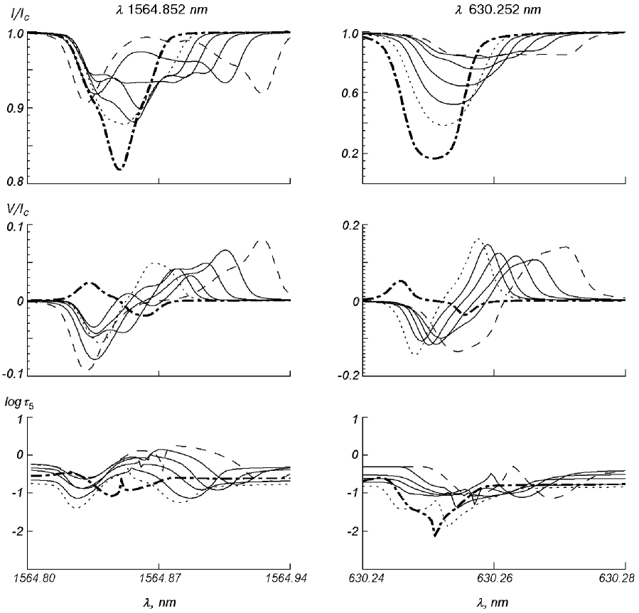
Figure 2: The Stokes I profiles (top panels) and the Stokes V profiles (middle panels) and the effective depths of V profile formation (lower panels) for lines $\lambda 1564.8$ nm and $\lambda 630.2$ nm calculated at a periphery of the fluxtube (solid line), its centre (dashed line), its edge (dotted line), and a granule centre (thick dash-and-dot line).

2) The relative distribution of magnetic field strength changes noticeably at different levels in the photosphere – a redistribution of fields in height takes place. The number of strong fields ($>100$ mT) decreases, and the distribution peak changes its position. At the photosphere base ($\log\tau_{5}=0$) the principal distribution maximum is indicative of the predominance of fields with strengths of about 25 mT. There is also a smaller peak near 100 mT and an even smaller one near 70 mT. At the level $\log\tau_{5}=$ -0.5 the fields become weaker, and the distribution has only one peak near 20 mT. At the levels $\log\tau_{5}=$ -1 and -1.5 the principal peak shifts toward weaker fields (about 10 mT), and a new peak of about the same height appears near 45 mT. The doubling of the principal peak is the manifestation of the canopy effect (strong fluxtubes expand with growing height). As a result, the contribution of strong fields of fluxtubes in the total number of fields increases. In still higher layers the field in fluxtubes expands even more and becomes weaker as well, and the distribution of weak fields becomes nearly the same as at the photosphere base. So, the MHD simulation results substantiate the view that magnetic fields become weaker with growing height in the photosphere and that the fields are subjected to redistribution.

3) Photospheric magnetic fields outside the active regions are a mixture of weak, moderate, and strong fields. Their strength can vary continuously from the lowest values in inclined fields which fill the entire granule region to the greatest values in the fields compressed into thin vertical fluxtubes which are found in intergranular lanes.

4) A comparison between the true distribution (obtained from MHD models) and the calculated distribution (obtained from profile synthesis) clearly shows that the method in which field strength is determined directly from the distance between the V profile peaks of the $\lambda$ 1564.8 nm line allows fields of 17 mT and greater to be measured. The number of measured fields is overestimated in the interval 20–50 mT, but for fields above 50 mT it agrees satisfactorily with actual numbers. It should be stressed that the number of fields with strengths of about 150 mT is estimated quite reliably by this method.

5) The field strength distribution derived from the $\lambda$ 630.2 nm line suggests that this line is unsuitable for the given method of field strength measurements. The distribution maximum corresponds to fields with $B\approx 100$ mT, which is at variance with the actual distribution.

We tried to find out why the distribution based on the $\lambda$ 1564.8 nm line profiles differs significantly from the actual distributions for fields below 50 mT and why the $\lambda$ 630.2 nm line is not suitable for such studies at all. With this in mind we analyzed in detail the cause of the variation in the V profile peak separation in nonhomogeneous models.

3 The reliability of the field strength distribution
obtained from the 1564.8 nm and 630.2 nm lines

Below we give some quantitative estimates for the accuracy of the field strength determinations based on the $\lambda$ 1564.8 nm and $\lambda$ 630.2 nm lines. Recall that the sensitivity of a line to a given magnetic field depends on the width ratio $\Delta\lambda_{B}{/}\Delta\lambda_{D}$, where $\Delta\lambda_{B}$ is the Zeeman splitting and $\Delta\lambda_{D}$ is the Doppler line width in the absence of magnetic fields. These widths depend on wavelength, temperature, line saturation, nonstationary velocities and their gradients. The Zeeman width also depends on the Landé factor as well as on the magnitudes and gradients of field strength and magnetic vector inclination. Hence it follows that the quantity $\Delta\lambda_{B}{/}\Delta\lambda_{D}$ for a specific magnetic field and a specific velocity field is a function of temperature and it grows approximately linearly with wavelength $\lambda$ and Landé factor $g_{\rm eff}$. The product $\lambda g_{\rm eff}$ is often taken as a measure of the sensitivity of spectral lines to magnetic field. In the atmospheric regions with widely different magnetic properties the trustworthiness of the field strength measured with the use of Zeeman splitting in a specific line depends on the magnetic sensitivity of the line (e.i., from $\lambda g_{\rm eff}$) as well as on the magnetic field parameters, in other words, it depends on the splitting conditions for the given line. The splitting conditions which are illustrated in [15, 20, 21, 24] are commonly divided into three groups. Soft conditions correspond to $\Delta\lambda_{B}<\Delta\lambda_{D}$, intermediate conditions to $\Delta\lambda_{B}\approx\Delta\lambda_{D}$, and hard ones to $\Delta\lambda_{B}>\Delta\lambda_{D}$. Special test calculations were made to establish these conditions for the two above lines and for our model atmosphere. We calculated the line profiles for one of the MHD model columns, having replaced the depth-dependent model field strengths by constant ones which varied from their smallest value to the greatest one. We also assumed that the fields were longitudinal. We calculated the field strength $B_{br}$ from the measured distances between the blue and the red V profile peaks and compared it to the actual field strengths (solid curves in Fig. 3). One can see that the conditions of strong splitting occur at $B>30$ mT for the $\lambda$ 1564.8 nm line and at $B>150$ mT for the $\lambda$ 630.2 nm line. The splitting is weak for all fields with $B<17$ mT for $\lambda$ 1564.8 nm and $B<60$ mT for $\lambda$ 630.2 nm. Under soft conditions, the measured field strength is determined by the Doppler width only and does not depend on any B variations – the threshold field strength is close to 20 mT for $\lambda$ 1564.8 nm and 90 mT for $\lambda$ 630.2 nm. In the case of intermediate conditions, the overestimate of field strengths is greater for weaker fields. We also examined the influence of the gradients of magnetic field, temperature, vertical velocity, and inclination on the conditions which set in one case or another. It turned out that the action of field gradient on profile shape is greater than on the distance between $|V|$ maxima. This distance is also only slightly affected by temperature and velocity gradients, but the field inclination exerts the greatest effect on the separation of V profile peaks. As seen from Fig. 3, an increase of field inclination extends the limits of the intermediate condition interval towards stronger fields, and the hard conditions set in at $B\approx 40$ mT for $\gamma=30^{\circ}$ and $B\approx 50$ mT for $\gamma=75^{\circ}$ in the case of the $\lambda$ 1564.8 nm line. This effect is even stronger for $\lambda$ 630.2 nm. As a result the field strength is overestimated still further, and the deviation of the measured field strengths from the actual ones is greater in more horizontal and weaker fields.

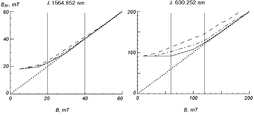
Figure 3: The field strengths $B_{br}$ derived from the distances between the V peaks of the synthesized profiles $\lambda 1564.8$ nm and $\lambda 630.2$ nm vs. the true (model) field strengths $B$ for magnetic vector inclination of $0^{\circ}$ (solid line), $30^{\circ}$ (dash-and-dot line), and $75^{\circ}$ (dashed line). Dotted line is line of equal field strengths. Vertical lines indicate the field strengths at which $\Delta\lambda_{B}{/}\Delta\lambda_{D}$ is equal to 1 (left line) and 2 (right line).

So, the direct method for the determination of $B$ from the distance between the $|$V$|$ profile maxima works better in the case of strong and longitudinal fields, and its accuracy deteriorates as the magnetic vector deviates from the vertical. For lines in the visible spectral range (like $\lambda$ 630.2 nm) the measured field strength can be overestimated by 20–40 mT for strongly inclined fields. The line $\lambda$ 630.2 nm can give trustworthy results only for strong-splitting conditions (fields above 150 mT) with inclinations less than $30^{\circ}$. In the case of weak-splitting conditions all measured fields will have a strength of about 100 mT. At the same time the effect of field inclination on measured strengths is insignificant for the $\lambda$ 1564.8 nm line. The greatest overestimate which is possible under intermediate-splitting conditions is about 2–4 mT for strongly inclined fields. The field inclination effect for $\lambda$ 1564.8 nm is 10 times weaker than for $\lambda$ 630.2 nm.

The accuracy of field strength measurements reflects directly on the field distributions, especially on those obtained for quiet regions, where inclined and weak fields dominate. In the case of soft conditions, when the magnetic sensitivity of lines is weak, weaker fields are measured as stronger ones (especially in the $\lambda$ 630.2 nm line). As a result the field distribution is considerably distorted in the region below 150 mT (for $\lambda$ 630.2 nm), while in the distribution derived with the use of the $\lambda$ 1564.8 nm line the region of weak fields between 20 and 40 mT is substantially distorted and the fields below 17 mT are absent at all. It is precisely these results that we obtained (see Fig. 1).

Hence it follows that in the case of complete resolution (filling factor $\alpha=1$) the most trustworthy field distribution is that which was found from the distance between the V peaks of $\lambda$ 1564.8 nm only under strong-field conditions, i.e., for strengths above 50 mT. The number of fields measured in the range -20–50 mT is overestimated: first, weak fields below 17 mT are measured as 20-mT fields and, second, the presence of inclined fields results in an overestimation by 2–4 mT. So, the main maximum of the field distribution found from the $\lambda$ 1564.8 nm line for quiet regions on the Sun is expected to be slightly shifted toward stronger fields with respect to the actual distribution, and it should also be higher at the expense of the fields from the weak-field conditions. It is most likely to be located at 30–40 mT. The field distribution beyond 50 mT up to the strongest kilogauss fields is not distorted.

In the cases when the spatial resolution is not high (filling factor $\alpha<1$), there is an additional profile broadening caused by the horizontal averaging of the profiles. This broadening also affects the shape of the distribution of measured fields, as judged from Fig. 4, which displays some distributions obtained from the $\lambda$ 1564.8 nm line (thick curve), and directly from MHD models (dotted line). The greater the spatial averaging scale, the greater is the shift of the distribution maximum toward stronger fields (30–40 mT); in addition, another maximum appears at 50–60 mT, the number of fields above 60 mT noticeably decreases, and the distribution shows a steeper decline toward stronger fields. In Fig. 4 we also give for comparison the observation data from [8] acquired with a resolution of 0.5–1^′′. The best agreement can be seen in the second panel, where the profile averaging seems to be close to the angular resolution of observations. Satisfactory agreement between our calculations and observations from [8] argues for the reliability of our calculations and distributions of weak fields on the quiet Sun.

As to the $\lambda$ 630.2 nm line, the distances between its peaks give a completely false distribution. This line can be used only to measure longitudinal fields above 150 mT. All fields below 100 mT are fixed as fields of 90–120 mT, and the resulting distribution has its maximum at $B=100$ mT. In actual practice this line is not used in the method discussed here. It is often used, as a rule, in the inverse codes, when a model atmosphere and a magnetic vector are found by comparing the observed and calculated V profiles. Our analysis shows that it is practically impossible to recognize the separation of the V peaks in weak profiles without additional analysis of the Q, U profiles at small field strengths and large magnetic vector inclinations. The inverse methods can give stronger longitudinal fields instead of weaker horizontal fields. It is not surprising, therefore, that the distributions obtained by inverse methods with the $\lambda$ 630.2 nm line have their maxima, as a rule, at 50–100 mT. We believe that the inverse methods need to be tested with the 2D MHD or 3D MHD models. Only then one may judge on the accuracy of the inversion.

4 Statistical properties of photospheric
magnetogranulation from the 1564.8 nm data

We consider the statistical relationships between the granule structure parameters derived from the synthesized $\lambda$ 1564.8 nm line profiles. Figures 4a and 4b display the field strength $B_{br}$ histograms and $B_{br}$ averaged over equal intervals as a function of the line-of-sight velocity $V_{z}$ derived from the V profile zero-crossing shift. Note that negative velocities correspond to downward motion. The field increases with the downflow velocity, and this suggests that the magnetic field becomes stronger in the intergranular lanes, where downflows are concentrated. The same is illustrated by the relation in Fig. 4c which points to an increase of field strength in darker photospheric regions where the contrast $I_{c}/{<}I_{c}{>}$ is less than unity. The field strength changes from $40\pm 25$ mT to $90\pm 40$ mT, on the average, when going from granules to intergranular lanes. Similar relations derived from observations [8] give 45 mT for granules and 69–80 mT for the lanes.

The radial velocity $V_{z}$ histograms (Fig. 5a) give a mean velocity of 0.37 km/s, which suggests the predominance of intense downflows. These downflows are associated with intergranular lanes, as suggested by close correlation between mean velocity and intensity contrast (Fig. 5c). A close relation between velocity and inclination should be also noted (Fig. 5b). Fields with greater inclinations are met mainly in the region of upflows, at sites with higher contrast, that is, at bright centers of granules. The asymmetry of radial velocity histograms and the correlation between velocity, inclination, and contrast bear out the fundamental property of magnetoconvection – the asymmetry of upward and downward flows of matter with frozen-in magnetic fields. As a result the magnetic field structure and the scale of magnetic field variations are closely related to the granulation dimensions and structure.

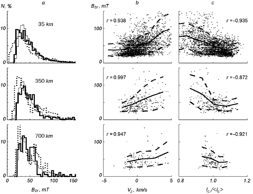
Figure 4: Magnetic field strength histograms (a) plotted with the use of the data from the synthesized $\lambda 1564.8$ nm line V profiles (thick line) and MHD models (dotted line) with different spatial averaging (35, 350, 700 km). The date of observations [8] with spatial resolution of 350–700 km idicate by thin line. Scatter plots of the field strength vs. radial velocity (b) and continuum intensity contrast (c). Solid lines are correlation curves, dashed lines are rms deviations; $r$ is the correlation coefficient.

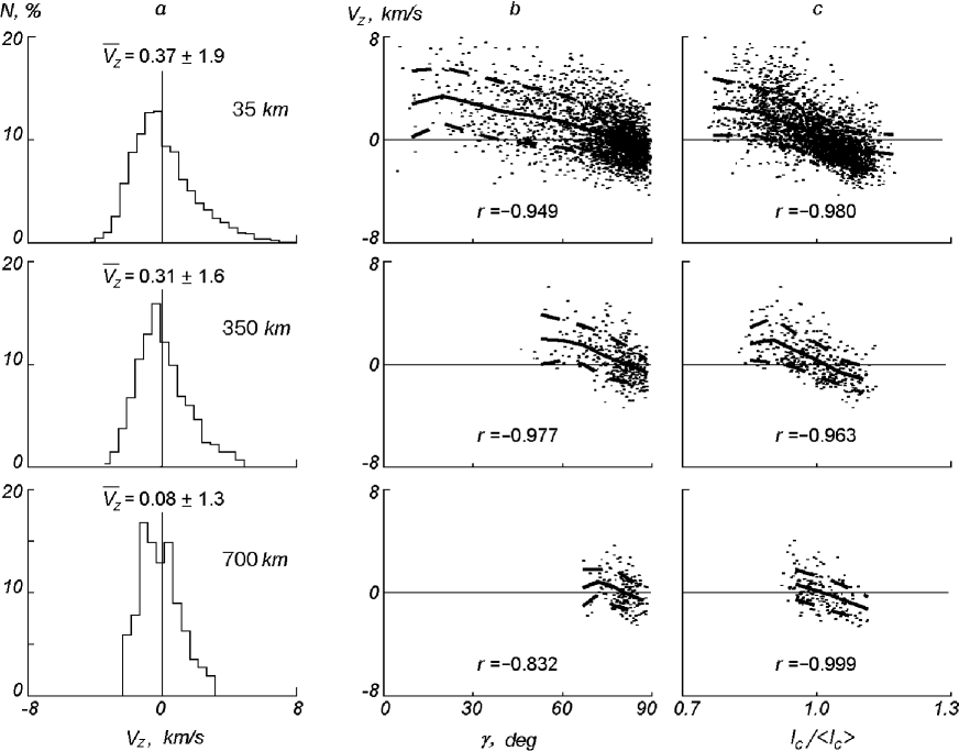
Figure 5: Histograms of radial velocities (a) derived from zero-crossing shifts of the synthesized $\lambda 1564.8$ nm line V profiles. Scatter plots of the radial velocities vs. magnetic vector inclination $\gamma$ derived from the relation $\tan^{2}\gamma={(Q^{2}+U^{2})}^{1/2}{/}V^{2}$ (b), and continuum intensity contrast $I_{c}/{<}I_{c}{>}$ (c). Symbol and curve coding are as in Firure 4.

As all observation data contain the results of the analysis of the asymmetry of observed Stokes profiles, we also give the corresponding data obtained from the synthesis of the $\lambda$ 1564.8 nm line V profiles in the form of histograms and scattering plots as well as the relations between the corresponding quantities averaged over equal intervals (Figs 6 and 7). To demonstrate the asymmetry, we took the standard parameter $\delta a=(a_{b}-a_{r}){/}(a_{b}+a_{r}$) which characterizes the amplitude asymmetry between the blue and red peaks of V profile. The sample-averaged asymmetry is positive and very small (Fig. 6a), but it grows with the scale of the spatial averaging of the profiles and approaches the observed values [8]. The $\lambda$ 1564.8 nm line asymmetry can change by $\pm 40$ percent, much less than in the $\lambda$ 630.2 nm line. This is evidence for a lower sensitivity of the former line to temperature and velocity gradients and magnetic vector variations. The area asymmetry $\delta A$ is measured in the same way as $\delta a$, and the relation between these quantities is demonstrated in Figs 6b,c. Figure 7 shows the correlation between the amplitude asymmetry $\delta a$ and other parameters. The smaller the field strength, the greater is the scatter of asymmetry parameter (Fig. 7a). The predominance of positive asymmetry tends to increase as the field strength grows (Fig. 7b). There is no well-defined relation between the asymmetry and radial velocity (Figs 7c,d), we can only notice that there are more profiles with positive asymmetry in upflow regions (negative velocities), while the number of profiles with negative asymmetry is slightly larger in downflow regions. This weak relationship breaks down as the spatial-averaging scale increases.

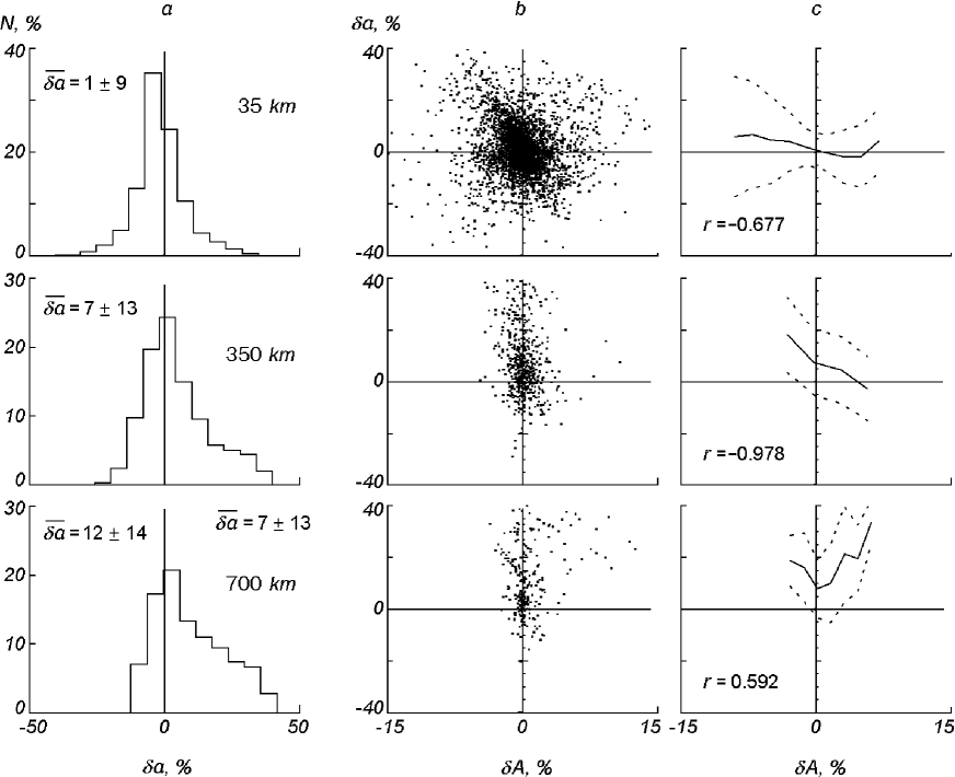
Figure 6: Histograms of the V profile amplitude asymmetry of the synthesized $\lambda 1564.8$ nm lines (a); scatter plots of the V profile amplitude asymmetry vs. the V profile area asymmetry (b); solid lines are corresponding correlation curves, dotted lines are rms deviations, and $r$ is the correlation coefficient (c).

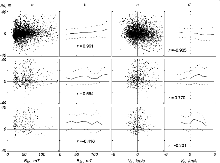
Figure 7: Scatter plots of the V profile amplitude asymmetry of the synthesized $\lambda 1564.8$ nm lines vs. magnetic field strength (a), radial velocity (c); corresponding correlation curves (b, d). Symbol and curve coding are as in Firure 6.

Note that Figures 4–7 also display the statistical relations for the parameters derived from the profiles averaged over 350-km and 700-km areas which correspond to resolutions of $0.5^{\prime\prime}$ and $1^{\prime\prime}$. The number of profiles drastically diminishes as the averaging scale grows, and the statistics results are less accurate, although the effects of the horizontal averaging of profiles can be still noticed in the figures. In some cases the results from the averaged profiles are in better agreement with observations.

5 Disbalance and distribution of magnetic flux

Disbalance of positive and negative magnetic fluxes is an important aspect of magnetic field distribution in the solar photosphere. It is defined as $\Delta F=(F^{+}+F^{-}){/}(|F^{+}|+|F^{-}|)$ [12], i.e., it is not affected by unresolved fluxes, since the spatial resolution acts in the same way on both flux components. We used this formula to calculate the magnetic flux disbalance in the model region as a function of time. The magnetic flux was calculated every minute for the 2D MHD models from the whole 30-min 2D MHD model sequence as $F=\Sigma_{i=1}^{N}B_{i}(\log\tau_{5}=0)\Delta x^{2}$, where $i$ is the model column number, $N=112$ is the number of columns in a 2D MHD model, and $\Delta x=35$ km is the column width. The field strengths $B_{i}$ at $\log\tau_{5}=0$ were taken from the data of magnetoconvection simulation [3].

Figure 8 shows the $\Delta F$ variation for 30 min. The smallest disbalance $\Delta F$ is 0.001 and the greatest one is 0.32. Time variations of $\Delta F$ display oscillatory behavior.

Figure 9 (top panel) shows the magnetic flux histogram derived from the whole 30-min MHD model sequence with $\Delta x=35$ km. The disbalance $\Delta F=-0.017$, the averaged field strength, or flux density, $\overline{B}=0.202$ mT, and the averaged unsigned field strength $\overline{|B|}=32$ mT. Figure 9 also shows our results obtained with other spatial resolution $\Delta x=350$ km (middle panel) and $\Delta x=700$ km (lower panel). The shape of flux distribution vary substantially, while the disbalance and mean field strength show insignificant variations.

We also try to compare our results with the measurements data of the general magnetic field (GMF) of the Sun [9], where the longitudinal field component for the Sun as a star is given. According to [9], the GMF strength characterizes the overbalance of the magnetic field of one polarization over the flux of the opposite polarization referred to a unit surface of the visible disk. Furthermore, the GMF is mainly controlled by the magnetic fluxes from vast areas which are not related to active regions. The contribution of active regions to the GMF is insignificant. The fields in such vast quiet areas were called background fields. The GMF strength (or the background fields) is 0.1–0.2 mT. We obtained $\overline{B}=-0.2$ mT, i.e., the absolute value the same as for the upper limit of observed field strengths. Although the agreement is quite good, it could be worse for various reasons. The measured GMF critically depends on magnetograph sensitivity and noise level. A twofold increase in the sensitivity results in nearly the same increase in the measured magnetic flux. Besides, the use of new calibration techniques in magnetic measurements also increases the measurement result (by a factor of 2.4) because old techniques did not take into consideration various factors: the saturation of lines in strong fields, when the V signal is not proportional to magnetic flux any more, the weakening of lines in regions with strong magnetic fields, and a partial compensation of the flux because of the presence of opposite polarities in the resolved surface element. In general, the measurement of the magnitude of the total solar flux with magnetographs with commonly low spatial resolution is assumed to give underestimated fluxes.

The present measurements of the photospheric magnetic fields with substantially higher accuracy [12, 13, 25] found their complex structure. The main components of these fields are network (N) and intranetwork (IN) fields. The N fields have strengths of about 100 mT and mixed polarities, they are mainly met at the corners of convective cells of supergranules and can form clusters. At solar minimum periods the network covers the solar surface. According to current measurements, the magnetic flux from network clusters is about $2\cdot 10^{10}$–$3\cdot 10^{11}$ Wb.

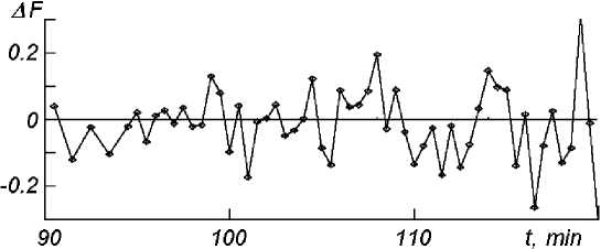
Figure 8: Magnetic flux disbalance calculated every minute from the 30-min 2D MHD model sequence as a function of simulation time.

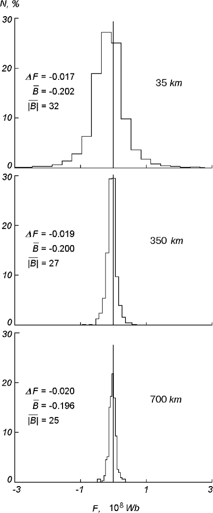
Figure 9: Magnetic flux distribution calculated with different spatial averaging (35, 350, 700 km) for the 30-min 2D MHD model sequence. Averaged field strengths are given in mT units.

With high sensitivity of polarimetric measurements and high spatial resolution at good seeing, weak fluxes from IN fields can be measured separately from the N fields. The IN fields are found inside the supergranulation network as big and small fragments. They are weaker and more diffuse, their fluxes are a factor of $10^{2}$ smaller than the fluxes from N fields. The mobility of IN fragments is higher, they are more free to move from the center of a supergranule to its boundaries. They can merge, annihilate one another, or interact with N fields. Being weak and having mixed polarities, the IN fields cannot penetrate to the outer chromosphere and corona. Observations of quiet regions with an spatial resolution of about $0.5^{\prime\prime}$ [12, 25] revealed that the mean flux density varied there from 0.3 to 4 mT. The IN fields contribute 0.165 mT to the mean flux density, which corresponds to a total solar flux of $10^{15}$ Wb. Since the lifetime of IN fragments is much less than one day, a flux of about $10^{16}$ Wb emerges from the Sun and disappears in the form of IN fields in one day. This flux is close to the total flux from the whole Sun observed at the maximum of solar cycle 21. According to [25], the disbalance of the IN field flux is 0.08 and the mean field strength is 0.59 mT, while the IN disbalance obtained in [12] varies from 0.03 to 0.48 depending on fragment observed, and it is smaller approximately by a factor of three than the N disbalance. Our magnetoconvection simulation gives the mean field strength of 0.2 mT and the flux disbalance of 0.02. It is less than the lower limit of the disbalance observed with high spatial resolution. The difference seems to be caused, on the one hand, by the fact that we use the results of 2D MHD simulation instead 3D MHD sinulation and, on the other hand, by insufficient accuracy of observations because of inadequate noise level and seeing conditions.

It should be noted that the extent of disbalance is also of importance in identifying the sources of weak IN fields [12]. The IN fields differ from the N fields not only by their properties but by their nature as well. As their disbalance is smaller, they are assumed [12] to originate from the local dynamo and not from the global convection circulation appropriate to the network fields. The authors of [22] ruled out the local surface dynamo as a mechanism of the IN field generation. The energy of weak small-scale fields in the surface layers grows due to field concentration rather than through the dynamo action, and the concentration of fields, their stretching and twisting are caused by convective motions. A 3D magnetoconvection simulation [22] demonstrated that under the conditions of strong stratification and asymmetric convective flows on the Sun a local short-period recirculation can arise near the surface. Such is the mechanism which can constantly sustain weak magnetic fields inside granules, mesogranules, and supergranules on the quiet Sun. Such a surface recirculation was also obtained in the study [14] based on the 2D magnetoconvection simulation [3]. The local surface short-period recirculation is favorable to rapid mixing of the fields of opposite polarities on small scales, thus diminishing the flux disbalance in the intranetwork fields. Today, the question of the nature of the magnetic IN field is open.

6 Conclusion

We used 2D MHD magnetogranulation models [3] with relatively high numerical resolution to investigate the magnetic field distribution in the solar photosphere outside the active regions and obtained the following results.

1. At the photosphere base the magnetic fields are predominantly weak, their strength is less than 50 mT. The strength distribution peak corresponds, on the average, to 25-mT fields. The distribution tail is rather long, it extends to 150 mT. There is another small peak at 100–110 mT, it suggests that such strengths dominate in kilogauss fields in network fluxtubes. The photospheric field distribution varies considerably with height, and this is evidence of a redistribution of the fields due to their weakening, on the one hand, and the expansion of fluxtubes, which increase the number of strong fields, on the other hand. All these data suggest that photospheric magnetic fields are a mixture of various fields, from the weakest ones to the strongest kilogauss fields of fluxtubes. Their strength can vary almost continuously from the lowest values in inclined fields in granules to the highest ones in thin vertical fluxtubes found in intergranular lanes. Alternating flux polarities produce a polarity disbalance about -0.02.

2. The direct measurement of magnetic field strength from the distance between the maxima in the $\lambda$ 1564.8 nm line profiles, providing a high spatial resolution ($\leq 0.5^{\prime\prime}$), is a very efficient and reliable tool for fields above 50 mT, but it fails for fields below 20 mT. All weak fields below 17 mT are measured as fields of 18–20 mT. In addition, the field strengths below 50 mT can be overestimated by 2–4 mT due to the effects of inclined fields which are ignored in this method. So, the relative distribution of fields above 50 mT acquired with the use of the $\lambda$ 1564.8 nm line with sufficiently high spatial resolution is close to the actual distribution and can serve as a standard in testing other spectral lines with this method or in testing other methods. The number of fields of 20–50 mT is always overestimated, and the existence of fields below 20 mT in quiet solar regions remains unnoticed in these distributions. Even with the complete resolution of magnetic fields this method applied to the $\lambda$ 1564.8 nm line, which is very sensitive to magnetic field, is unsuitable for measuring very weak fields below 20 mT.

3. The inverse methods in which the strengths of weak magnetic fields are determined from the Stokes V profiles of the visible lines like $\lambda$ 630.2 nm also seem to overestimate the field strengths as compared to the methods based on the IR lines like $\lambda$ 1564.8 nm. A possible reason is the weak magnetic sensitivity of $\lambda$ 630.2 nm to fields below 150 mT, on the one hand, and its high sensitivity to magnetic vector inclination, on the other hand. It is difficult to separate the field strength effect from the field inclination effect on the V profile shape and the distance between profile peaks without making recourse to the Q and U profiles. The field inclination effect for the $\lambda$ 630.2 nm line is nearly 10 times stronger than for the $\lambda$ 1564.8 nm line. Therefore, the field distributions found with the use of the $\lambda$ 630.2 nm line for quiet photospheric regions, where the fields are predominantly inclined, are less reliable, especially for subkilogauss fields, compared to the distributions found with the $\lambda$ 1564.8 nm line. The high sensitivity of $\lambda$ 630.2 nm to magnetic vector inclination can be successfully used for the diagnostics of this field parameter.

Acknowledgements.We wish to thank S. Solanki and E. Khomenko for making available the observation data on magnetic field distributions. This study was carried out within the framework of an international research program and was made possible in part by the INTAS Grant No. 0084.

References

- [1] M. Collados, Infrared polarimetry, in: Advanced Solar Polarimetry – Theory, Observation, and Instrumentation, M. Sigwarth (Editor), ASP Conf. Ser., vol. 236, pp. 255–271, 2001.
- [2] T. Emonet and F. Cattaneo, Small-scale photosphere fields: observational evidence and numerical simulation, Astrophys. J., vol. 560, no. 2, pp. L197–L200, 2001.
- [3] A. S. Gadun, Two-dimensional nonstationary maghetogranulation, Kinematika i Fizika Nebes. Tel [Kinematics and Physics of Celestial Bodies], vol. 16, no. 2, pp. 99–120, 2000.
- [4] A. S. Gadun, V. A. Sheminova, and S. K. Solanki, Formation of small-scale magnetic elements: surface mechanism, ibid., vol. 15, no. 5, pp. 387–397, 1999.
- [5] A. S. Gadun, S. K. Solanki, V. A. Sheminova, and S. R. O. Ploner, A formation mechanism of magnetic elements in regions of mixed polarity, Solar Phys., vol. 203, no. 1, pp. 1–7, 2001.
- [6] U. Grossmann-Doerth, C. U. Keller, and M. Schussler, Observations of the quiet Sun’s magnetic field, Astron. and Astrophys., vol. 315, no. 3, pp. 610–617, 1996.
- [7] C. U. Keller, F. -L. Deubner, U. Egger, et al., On the strength of solar intra-network fields, ibid., vol. 286, no. 2, pp. 626–634, 1994.
- [8] E. V. Khomenko, M. Collados, A. Lagg, et al., Statistical properties of magnetic fields in intranetwork, in: SOLMAG 2002: Proc. of the Magnetic Coupling of the Solar Atmosphere Euroconference and IAU Colloquium 188, Santorini, Greece, 11–15 June 2002, pp. 445–448 (ESA SP-505, October 2002).
- [9] V. A. Kotov, N. N. Stepanyan, and Z. A. Shcherbakova, The role of the background magnetic field and the fields in active regions and sunspots in the general magnetic field of the Sun, Izv. Krym. Astrofiz. Observ., vol. 56, pp. 75–83, 1977.
- [10] H. Lin, On the distribution of the solar magnetic fields, Astrophys. J., vol. 446, no. 1, pp. 421–430, 1995.
- [11] H. Lin and T. Rimmele, The granular magnetic fields of the quiet Sun, ibid., vol. 514, no. 1, pp. 448–455, 1999.
- [12] B. W. Lites, Characterization of magnetic flux in the quiet Sun, ibid., vol. 573, no. 1, pp. 431–444, 2002.
- [13] F. S. Martin, The indication and interaction of network, intranetwork, and ephemeral-region magnetic fields, Solar Phys., vol. 117, no. 2, pp. 243–259, 1988.
- [14] S. R. O. Ploner, M. Schüssler, S. K. Solanki, and A. S. Gadun, An example of reconnection and magnetic flux recycling near the solar surface, in: Advanced Solar Polarimetry – Theory, Observation, and Instrumentation, M. Sigwarth (Editor), ASP Conf. Ser., vol. 236, pp. 363–370, 2001.
- [15] D. Rabin, Spatially extended measurements of magnetic field strength in solar plage, Astron. and Astrophys., vol. 391, no. 2, pp. 832–844, 1992.
- [16] J. Sanchez Almeida and B. W. Lites, Physical properties of the solar magnetic photosphere under the MISMA hypothesis. II. Network and internetwork fields at the disk center, Astrohys. J., vol. 532, no. 2, pp. 1215–1229, 2000.
- [17] V. A. Sheminova, Depths of formation of magnetically sensitive absorption lines in the solar atmosphere, Kinematika i Fizika Nebes. Tel [Kinematics and Physics of Celestial Bodies], vol. 8, no. 3, pp. 44–62, 1992.
- [18] V. A. Sheminova, Two-dimensional MHD models of solar magnetogranulation. Testing of models and methods of Stokes diagnostics, ibid., vol. 15, no. 5, pp. 398–411, 1999.
- [19] H. Socas-Navarro and J. Sanchez Almeida, Magnetic properties of photospheric regions with very low magnetic flux, ibid., vol. 565, no. 2, pp. 1323–1334, 2002.
- [20] S. K. Solanki, Small-scale solar magnetic fields: an overview, Space Sci. Rev., vol. 31, p. 188, 1993.
- [21] S. K. Solanki, I. Rüedi, and W. Livingston, Infrared lines as probes of solar magnetic features. II. Diagnostic capabilities of Fe I 15648.5 Å and 15652.9 Å, Astron. and Astrophys., vol. 263, no. 1/2, pp. 312–322, 1992.
- [22] R. F. Stein and Å. Nordlung, Solar surface magneto-convection and dynamo action, in: SOLMAG 2002: Proc. of the Magnetic Coupling of the Solar Atmosphere Euroconference and IAU Colloquium 188, Santorini, Greece, 11–15 June 2002, pp. 83–89 (ESA SP-505, October 2002).
- [23] J. O. Stenflo, C. U. Keller, and A. Gandorfer, Differential Hanle effect and the spatial variation of turbulent magnetic fields on the Sun, Astron. and Astrophys., vol. 329, no. 1, pp. 319–328, 1998.
- [24] J. O. Stenflo, S. K. Solanki, and J. W. Harvey, Diagnostic of solar magnetic fluxtubes with the infrared line Fe 15648 A, ibid., vol. 173, no. 1, pp. 167–179, 1987.
- [25] J. Wang, H. Wang, F. Tang, et al., Flux distribution of solar intranetwork magnetic fields, Solar Phys., vol. 160, no. 2, pp. 227–288, 1995.