Correlation analysis of enzymatic reaction of a single protein molecule

Abstract

New advances in nano sciences open the door for scientists to study biological processes on a microscopic molecule-by-molecule basis. Recent single-molecule biophysical experiments on enzyme systems, in particular, reveal that enzyme molecules behave fundamentally differently from what classical model predicts. A stochastic network model was previously proposed to explain the experimental discovery. This paper conducts detailed theoretical and data analyses of the stochastic network model, focusing on the correlation structure of the successive reaction times of a single enzyme molecule. We investigate the correlation of experimental fluorescence intensity and the correlation of enzymatic reaction times, and examine the role of substrate concentration in enzymatic reactions. Our study shows that the stochastic network model is capable of explaining the experimental data in depth.

T1Supported in part by NSF Grant DMS-04-49204 and NIH/NIGMS Grant R01GM090202.

and

1 Introduction

In a chemical reaction, the number of molecules involved can drastically vary from millions of moles—a forest devastated by a fire—to only a few—reactions in a living cell. While most conventional chemical experiments were designed for a large ensemble in which only the average could be observed, chemistry textbooks tend to explain what really happens in a reaction on a molecule-by-molecule basis. This extrapolation certainly requires the homogeneity assumption: each molecule behaves in the same way, so the average also represents individual behavior. To verify this assumption, the kinetic of a single molecule must be directly observed, which requires rather sophisticated technology not available until the 1990s. Since then, the development of nanotechnology has enabled scientists to track and manipulate molecules one by one. A new age of single-molecule experiments began [Nie and Zare (1997), Xie and Trautman (1998), Xie and Lu (1999), Tamarat et al. (2000), Weiss (2000), Moerner (2002), Flomembom et al. (2005), Kou, Xie and Liu (2005), Kou (2009)].

Such experiments offer a greatly amplified view of single-molecular dynamics over considerably long time periods from seconds to hours, a time scale that far exceeds what can be achieved by computer based molecular dynamic simulation (even with a super computer, molecular dynamic simulation cannot reach beyond milliseconds). The single-molecule experiments also provide detailed information on the intermediate transition steps of a biological process not available in traditional experiments. Not surprisingly, these experiments reveal the stochastic nature of nanoscale particles long masked by ensemble averages: rather than remain rigid, those particles undergo dramatic conformation change driven by external thermal motion. Future development in this area will provide us a deeper understanding of biological processes [such as molecular motors, Asbury, Fehr and Block (2003)] and accelerate new technology development [such as single-molecule gene sequencing, Pushkarev, Neff and Quake (2009)].

Among bio-molecules, enzymes play an important role: by lowering the energy barrier between the reactant and product, they ensure that many life essential processes can be effectively carried out in a living cell. An aspiration of bioengineers is to artificially design and produce new and efficient enzymes for specific use. Studying and understanding the mechanism of existing enzymes, therefore, remains one of the central topics in life science. According to the classical literature, the kinetic of an enzyme is described by the Michaelis–Menten mechanism [Atkins and de Paula (2002)]: an enzyme molecule $E$ could bind with a reactant molecule $S$, which is referred to as a substrate in the chemistry literature (hence the symbol $S$), to form a complex $\mathit{ES}$. The complex can either dissociate to enzyme and substrate molecules or undergo a catalytic process to release the product $P$. The enzyme then returns to the original state $E$ to start another catalytic circle. This process is typically diagrammed as

$$E+S\mathop{\stackrel{{\scriptstyle k_{1}[S]}}{{\rightleftarrows}}}_{k_{-1}}\mathit{ES}\stackrel{{\scriptstyle k_{2}}}{{\rightarrow}}E^{0}+P,\qquad E^{0}\stackrel{{\scriptstyle\delta}}{{\rightarrow}}E,$$ (1)

where $[S]$ is the substrate concentration ($E^{0}$ is the release state of the enzyme), $k_{1}$ is the association rate per unit substrate concentration, $k_{-1}$ and $k_{2}$ are, respectively, the dissociation and catalytic rate, and $\delta$ is the returning rate. All the transitions are memoryless in the Michaelis–Menten scheme, so the whole process can be modeled as a continuous-time Markov chain consisting of three states $E$, $\mathit{ES}$ and $E^{0}$ for an enzyme molecule.

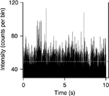
A recent single-molecule experiment [English et al. (2006)] conducted by the Xie group at Harvard University (Department of Chemistry and Chemical Biology) studied the enzyme $\beta$-galactosidase ($\beta$-gal), which catalyzes the breakdown of the sugar lactose and is essential in the human body [Jacobson et al. (1994), Dorland (2003)]. In the experiment a single $\beta$-gal molecule is immobilized (by linking to a bead bound on a glass coverslip) and immersed in buffer solution of the substrate molecules. This setup allows $\beta$-gal’s enzymatic action to be continuously monitored under a fluorescence microscope. To detect the individual turnovers, that is, the enzyme’s switching from the $E$ state to the $E^{0}$ state, careful design and special treatment were carried out (such as the use of photogenic substrate resorun-$\beta$-D-galactopyranoside) so that once the experimental system was placed under a laser beam the reaction product and only the reaction product was fluorescent. This setting ensures that as the $\beta$-gal enzyme catalyzes substrate molecules one after another, a strong fluorescence signal is emitted and detected only when a product is released, that is, only when the reaction reaches the $E^{0}+P$ stage in (1). Recording the fluorescence intensity over time thus enables the experimental determination of individual turnovers. A sample fluorescence intensity trajectory from this experiment is shown in Figure 1. High spikes in the trajectory are the results of intense photon burst at the $E^{0}+P$ state, while low readings correspond to the $E$ or $\mathit{ES}$ state. The time lag between two adjacent high fluorescence spikes is the enzymatic turnover time, that is, the time to complete a catalytic circle.

Figure 1: Fluorescence intensity reading from one experiment (the substrate concentration is 100 micro-molar). Each fluorescence intensity spike is caused by the release of a reaction product.

Figure 2: Left column: experimentally observed fluorescence intensity and turnover time autocorrelations under different substrate concentrations $[S]$ (20, 100 and 380 micromolar). Right column: the autocorrelations predicted by the classical Michaelis–Menten model. Under the Michaelis–Menten model, the turnover time autocorrelation should be zero and the intensity autocorrelations should decay exponentially and decay faster under larger concentration. All contradict the experimental findings.

Examining the experimental data, including the distribution and autocorrelation of the turnover times as well as the fluorescence intensity autocorrelation, researchers were surprised that the experimental data showed a considerable departure from the Michaelis–Menten mechanism. Section 2 describes the experimental findings in detail. Figure 2 illustrates the discrepancy between the experimental data and the Michaelis–Menten model in terms of the autocorrelations. The left two panels show the experimentally observed fluorescence intensity autocorrelation and turnover time autocorrelation under different substrate concentrations $[S]$. The right two panels show the corresponding autocorrelation patterns predicted by the Michaelis–Menten model. Comparing the bottom two panels, we note that under the classical Michaelis–Menten model the turnover time autocorrelation should be zero (hence the horizontal line at the bottom-right panel), which clearly contradicts the experimental result on the left. From the top two panels we note that under the Michaelis–Menten model the fluorescence intensity autocorrelation should decay exponentially and should decay faster with larger substrate concentration, but the experimental result shows the opposite: the intensity autocorrelations decay slower with larger substrate concentration, and they do not decay exponentially.

To explain the experimental puzzle, a new stochastic network model was introduced [Kou et al. (2005), Kou (2008b)], and it was shown that the stochastic network model well explained the experimental distribution of the turnover times. The autocorrelation of successive turnover times and the correlation of experimental fluorescence intensity, however, were not investigated in the previous articles.

This paper further explores the stochastic network model, concentrating on the correlation structure of the turnover times and that of the fluorescence intensity. The rest of the paper is organized as follows. Section 2 reviews the preceding work, including the experiment observation and the new stochastic network model. Section 3 analytically calculates the turnover time autocorrelation and the fluorescence intensity autocorrelation based on the stochastic network model. These analytical results give an explanation of the multi-exponentially decay pattern of the autocorrelation functions. Section 4 discusses how to fit the experiment data within the framework of the stochastic network model. The paper ends in Section 5 with a summary and some concluding remarks.

2 Modeling enzymatic reaction

2.1 The classical model and its challenge

Under the classical Michaelis–Menten model (1), an enzyme molecule behaves as a three-state continuous-time Markov chain with the generating matrix (infinitesimal generator)

$$\mathbf{Q}_{\mathrm{MM}}=\pmatrix{-k_{1}[S]&k_{1}[S]&0\cr k_{-1}&-(k_{-1}+k_{2})&k_{2}\cr\delta&0&-\delta}.$$

We can readily draw two properties from this continuous-time Markov chain model.

Proposition 2.1

The density function of the turnover time, the time that it takes the enzyme to complete one catalytic cycle (i.e., to go from state $E$ to state $E^{0}$), is

$$f(t)=\frac{k_{1}k_{2}[S]}{2p}\bigl{(}e^{-(q-p)t}-e^{-(q+p)t}\bigr{)},$$

where $p=\sqrt{(k_{1}[S]+k_{2}+k_{-1})^{2}/4-k_{1}k_{2}[S]}$ and $q=(k_{1}[S]+k_{2}+k_{-1})/2$.

Proposition 2.2

The successive turnover times have no correlation.

The first proposition implies that the density of turnover time is almost an exponential, since the term $e^{-(q-p)t}$ easily dominates the term $e^{-(q+p)t}$ for most values of $t$; see Kou (2008b) for a proof. The second proposition is a consequence of the Markov property: each turnover time, which is a first passage time, is independently and identically distributed.

The third property concerns the autocorrelation of the fluorescence intensity. As we have seen in Figure 1, the experimentally recorded fluorescence intensity consists of high spikes and low readings. The high peaks correspond to the release of the fluorescent product (when the enzyme is at the state $E^{0}$), whereas the low readings come from the background noise. We can thus think of the fluorescence intensity reading as a record of an on–off system: $E^{0}$ being the on state, $E$ and $\mathit{ES}$ being the off states.

Proposition 2.3

The autocorrelation function of the fluorescence intensity is proportional to $\exp(-t(k_{-1}+k_{2}+k_{1}[S]))$.

The proof of the proposition will be given in Corollary 3.11. This proposition says that under the Michaelis–Menten model the intensity autocorrelation decays exponentially and faster with larger substrate concentration $[S]$.

The results from the single-molecule experiment on $\beta$-gal [English et al. (2006)] contradict all three properties of the Michaelis–Menten model:

(1) The empirical distribution of the turnover time does not exhibit exponential decay; see Kou (2008b) for a detailed explanation.

(2) The experimental turnover time autocorrelations are far from zero, as seen in Figure 2.

(3) The experimental intensity autocorrelations decay neither exponentially nor faster under larger concentration. See Figure 2.

2.2 A stochastic network model

We believe these contradictions are rooted in the molecule’s dynamic conformational fluctuation. An enzyme molecule is not rigid: it experiences constant changes and fluctuations in its three-dimensional shape and configuration due to the entropic and atomic forces at the nano scale [Kou and Xie (2004), Kou (2008a)]. Although for a large ensemble of molecules, the (nanoscale) conformational fluctuation is buried in the macroscopic population average, for a single molecule the conformational fluctuation can be much more pronounced: different conformations could have different chemical properties, resulting in time-varying performance of the enzyme, which can be studied in the single-molecule experiment. The following stochastic network model [Kou et al. (2005)] was developed with this idea:

$$S+E_{1}\mathop{\stackrel{{\scriptstyle k_{11}[S]}}{{\rightleftarrows}}}_{k_{-11}}\mathit{ES}_{1}\stackrel{{\scriptstyle k_{21}}}{{\rightarrow}}P+E_{1}^{0},\qquad E_{1}^{0}\stackrel{{\scriptstyle\delta_{1}}}{{\rightarrow}}E_{1},$$

$$\hphantom{S}\downarrow\uparrow\hskip 37.0pt\downarrow\uparrow\hskip 30.0pt\hphantom{0}\downarrow\uparrow\qquad\hskip 10.0pt\hphantom{0}\cdots$$

$$S+E_{2}\mathop{\stackrel{{\scriptstyle k_{12}[S]}}{{\rightleftarrows}}}_{k_{-12}}\mathit{ES}_{2}\stackrel{{\scriptstyle k_{22}}}{{\rightarrow}}P+E_{2}^{0},\qquad E_{2}^{0}\stackrel{{\scriptstyle\delta_{2}}}{{\rightarrow}}E_{2},$$ (2)

$$\hphantom{S}\hskip 1.5pt\cdots\hskip 37.0pt\cdots\hskip 33.5pt\hphantom{0}\cdots\qquad\hskip 10.5pt\hphantom{0}\cdots$$

$$\hphantom{S}\downarrow\uparrow\hskip 37.0pt\downarrow\uparrow\hskip 30.0pt\hphantom{0}\downarrow\uparrow\qquad\hskip 10.0pt\hphantom{0}\cdots$$

$$S+E_{n}\mathop{\stackrel{{\scriptstyle k_{1n}[S]}}{{\rightleftarrows}}}_{k_{-1n}}\mathit{ES}_{n}\stackrel{{\scriptstyle k_{2n}}}{{\rightarrow}}P+E_{n}^{0},\qquad E_{n}^{0}\stackrel{{\scriptstyle\delta_{n}}}{{\rightarrow}}E_{n}.$$

This is still a Markov chain model but with $3n$ states instead of three. The enzyme still exists as a free enzyme $E$, an enzyme–substrate complex $\mathit{ES}$ or a returning enzyme $E^{0}$, but it can take $n$ different conformations indexed by subscripts in each stage. At each transition, the enzyme can either change its conformation within the same stage (such as $E_{i}\rightarrow E_{j}$ or $\mathit{ES}_{i}\rightarrow\mathit{ES}_{j}$) or carry out one chemical step, that is, move between the stages (such as $E_{i}\rightarrow\mathit{ES}_{i}$, $\mathit{ES}_{i}\rightarrow E_{i}$ or $\mathit{ES}_{i}\rightarrow E_{i}^{0}$). Since only the product $P$ is fluorescent in the experiment, in model (2.2) any state $E_{i}^{0}$ is an on-state, and the others are off-states. Consequently, the turnover time is the traverse time between any two on-states $E_{j}^{0}$ and $E_{k}^{0}$.

To fully specify the model, we need to stipulate the transition rates. For $i\neq j$, we use $\alpha_{ij}$, $\beta_{ij}$ and $\gamma_{ij}$ to denote, respectively, the transition rates of $E_{i}\rightarrow E_{j}$, $\mathit{ES}_{i}\rightarrow\mathit{ES}_{j}$ and $E_{i}^{0}\rightarrow E_{j}^{0}$. $k_{1i}[S]$, $k_{-1i}$, $k_{2i}$ and $\delta_{i}$ are, respectively, the transition rates of $E_{i}\rightarrow\mathit{ES}_{i}$, $\mathit{ES}_{i}\rightarrow E_{i}$, $\mathit{ES}_{i}\rightarrow E_{i}^{0}$ and $E_{i}^{0}\rightarrow E_{i}$. Define $\mathbf{Q}_{AA}$, $\mathbf{Q}_{BB}$ and $\mathbf{Q}_{CC}$ to be square matrices:

$$\mathbf{Q}_{AA}=[\alpha_{ij}]_{n\times n},\qquad\mathbf{Q}_{BB}=[\beta_{ij}]_{n\times n},\qquad\mathbf{Q}_{CC}=[\gamma_{ij}]_{n\times n},$$

where $\alpha_{ii}=-\sum_{j\neq i}\alpha_{ij}$, $\beta_{ii}=-\sum_{j\neq i}\beta_{ij}$ and $\gamma_{ii}=-\sum_{j\neq i}\gamma_{ij}$. They correspond to transitions among the $E_{i}$ states, among the $\mathit{ES}_{i}$ states and among the $E_{i}^{0}$ states, respectively. Define diagonal matrices

$$\qquad\mathbf{Q}_{AB} = \operatorname{diag}\{k_{11}[S],k_{12}[S],\ldots,k_{1n}[S]\},$$

$$\mathbf{Q}_{BA} = \operatorname{diag}\{k_{-11},k_{-12},\ldots,k_{-1n}\},$$

$$\mathbf{Q}_{BC} = \operatorname{diag}\{k_{21},k_{22},\ldots,k_{2n}\},$$

$$\mathbf{Q}_{CA} = \operatorname{diag}\{\delta_{1},\delta_{2},\ldots,\delta_{n}\}.$$

They correspond to transitions between the different stages. The generating matrix of model (2.2) is then

$$\quad\mathbf{Q}=\pmatrix{\mathbf{Q}_{AA}-\mathbf{Q}_{AB}&\mathbf{Q}_{AB}&\mathbf{0}\cr\mathbf{Q}_{BA}&\mathbf{Q}_{BB}-(\mathbf{Q}_{BA}+\mathbf{Q}_{BC})&\mathbf{Q}_{BC}\cr\mathbf{Q}_{CA}&\mathbf{0}&\mathbf{Q}_{CC}-\mathbf{Q}_{CA}}.$$ (4)

Under this new model, the distribution of the turnover time, the correlation of turnover times and the correlation of the fluorescence intensity can be analyzed and compared with experimental data. This paper studies the autocorrelation of turnover time and the autocorrelation of fluorescence intensity.

3 Autocorrelation of turnover time and of fluorescence intensity

3.1 Dynamic equilibrium and stationary distribution

In the chemistry literature, the term “equilibrium” often refers to the state in which all the macroscopic quantities of a system are time-independent. For the microscopic system studied in single-molecule experiments, macroscopic quantities, however, are meaningless, and microscopic parameters never cease to fluctuate. Nonetheless, for a micro-system, one can talk about dynamic equilibrium in the sense that the distribution of the state quantities become time-independent, that is, they reach the stationary distribution. The single-molecule enzyme experiment that we consider here falls into this category, since the enzymatic reactions happen quite fast. We cite the following lemma [Lemma 3.1 of Kou (2008b)], which gives the stationary distribution of the Markov chain (2.2):

Lemma 3.1

Let $X(t)$ be the process evolving according to (2.2). Suppose all the parameters $k_{1i},k_{-1i},k_{2i},\delta_{i},\alpha_{ij},\beta_{ij}$, and $\gamma_{ij}$ are positive. Then $X(t)$ is ergodic. Let the row vectors $\bolds{\pi}_{A}=(\pi(E_{1}),\pi(E_{2}),\ldots,\pi(E_{n}))$, $\bolds{\pi}_{B}=(\pi(\mathit{ES}_{1}),\ldots,\pi(\mathit{ES}_{n}))$, and $\bolds{\pi}_{C}=(\pi(E_{1}^{0}),\ldots,\pi(E_{n}^{0}))$ denote the stationary distribution of the entire network. Up to a normalizing constant, they are determined by

$$\displaystyle\bolds{\pi}_{A}=-\bolds{\pi}_{C}\mathbf{Q}_{CA}\mathbf{L},\qquad\bolds{\pi}_{B}=-\bolds{\pi}_{C}\mathbf{Q}_{CA}\mathbf{M},$$

$$\displaystyle\bolds{\pi}_{C}(\mathbf{Q}_{CC}-\mathbf{Q}_{CA}-\mathbf{Q}_{CA}\mathbf{MQ}_{BC})=0,$$

where the matrices

$$\mathbf{L} = [\mathbf{Q}_{AA}-\mathbf{Q}_{AB}-\mathbf{Q}_{AB}(\mathbf{Q}_{BB}-\mathbf{Q}_{BA}-\mathbf{Q}_{BC})^{-1}\mathbf{Q}_{BA}]^{-1},$$

$$\mathbf{M} = [\mathbf{Q}_{BB}-\mathbf{Q}_{BC}-(\mathbf{Q}_{BB}-\mathbf{Q}_{BA}-\mathbf{Q}_{BC})\mathbf{Q}_{AB}^{-1}\mathbf{Q}_{AA}]^{-1}.$$

Under the stochastic network model (2.2), a turnover event can start from any state $E_{i}$ and end in any $E_{j}^{0}$. It follows that the overall distribution of all the turnover times is characterized by a mixture distribution with the weights given by the stationary probability of a turnover event’s starting from $E_{i}$. The following lemma, based on Lemma 3.4 of Kou (2008b), provides the stationary probability.

Lemma 3.2

Let $\mathbf{w}$ be a row vector, $\mathbf{w}=(w(E_{1}),w(E_{2}),\ldots,w(E_{n}))$, where $w(E_{i})$ denotes the stationary probability of a turnover event’s starting from state $E_{i}$. Then up to a normalizing constant, $\mathbf{w}$ is the nonzero solution of

$$\mathbf{w}(\mathbf{I}+\mathbf{MQ}_{BC}-\mathbf{Q}_{CA}^{-1}\mathbf{Q}_{CC})=0.$$ (5)

3.2 Autocorrelation of turnover time

Expectation of turnover time

The enzyme turnover event occurs one after another. Each can start from any $E_{i}$ and end in any $E_{j}^{0}$. The next turnover may start from $E_{k}$ ($k\neq j$) when the system exits the $E^{0}$ stage from $E_{k}^{0}$. To calculate the correlation between turnover times, it is necessary to find out the probabilities of all these combinations and the expected turnover times. We introduce the following notation.

Let $T_{E_{i}}$ and $T_{\mathit{ES}_{i}}$ denote the first passage time of reaching the set $\{E_{1}^{0},\allowbreak E_{2}^{0},\ldots,E_{n}^{0}\}$ from $E_{i}$ and $\mathit{ES}_{i}$, respectively. Let $P_{E_{i}E_{j}^{0}}$ and $P_{\mathit{ES}_{i}E_{j}^{0}}$ be the probability that a turnover event, starting, respectively, from $E_{i}$ and $\mathit{ES}_{i}$, ends in $E_{j}^{0}$. Let $P_{E_{i}^{0}E_{j}}$ denote the probability that, after the previous turnover ends in $E_{i}^{0}$, a new turnover event starts from $E_{j}$. Finally, let $T_{E_{i}E_{j}^{0}}$ and $T_{\mathit{ES}_{i}E_{j}^{0}}$ be the first passage time of reaching the state $E_{j}^{0}$ from $E_{i}$ and $\mathit{ES}_{i}$, respectively.

For the values of $E(T_{E_{i}})$ and $E(T_{\mathit{ES}_{i}})$, we cite the following lemma [Corollary 3.3 of Kou (2008b)].

Lemma 3.3

Let the vectors $\bolds{\mu}_{A}=(E(T_{E_{1}}),E(T_{E_{2}}),\ldots,E(T_{E_{n}}))^{T}$ and $\bolds{\mu}_{B}=(E(T_{\mathit{ES}_{1}}),\ldots,E(T_{\mathit{ES}_{n}}))^{T}$ denote the mean first passage times. Then they are given by

$$\pmatrix{\bolds{\mu}_{A}\cr\bolds{\mu}_{B}}=\pmatrix{-(\mathbf{L}+\mathbf{M})\mathbf{1}\cr-(\mathbf{N}+\mathbf{R})\mathbf{1}},$$ (6)

where the matrices $\mathbf{N}$ and $\mathbf{R}$ are given by

$$\mathbf{N} = [\mathbf{Q}_{AA}-(\mathbf{Q}_{AA}-\mathbf{Q}_{AB})\mathbf{Q}_{BA}^{-1}(\mathbf{Q}_{BB}-\mathbf{Q}_{BC})]^{-1},$$

$$\mathbf{R} = [\mathbf{Q}_{BB}-\mathbf{Q}_{BA}-\mathbf{Q}_{BC}-\mathbf{Q}_{BA}(\mathbf{Q}_{AA}-\mathbf{Q}_{AB})^{-1}\mathbf{Q}_{AB}]^{-1}.$$

For the probabilities $P_{E_{i}E_{j}^{0}}$, $P_{\mathit{ES}_{i}E_{j}^{0}}$ and $P_{E_{i}^{0}E_{j}}$, we have the following lemma:

Lemma 3.4

Let $\mathbf{P}_{AC}$, $\mathbf{P}_{BC}$ and $\mathbf{P}_{CA}$ be probability matrices $\mathbf{P}_{AC}=[P_{E_{i}E_{j}^{0}}]_{n\times n}$, $\mathbf{P}_{BC}=[P_{\mathit{ES}_{i}E_{j}^{0}}]_{n\times n}$ and $\mathbf{P}_{CA}=[P_{E_{i}^{0}E_{j}}]_{n\times n}$. Then they are given by

$$\mathbf{P}_{AC}=-\mathbf{MQ}_{BC},\qquad\mathbf{P}_{BC}=-\mathbf{RQ}_{BC},\qquad\mathbf{P}_{CA}=(\mathbf{I}-\mathbf{Q}_{CA}^{-1}\mathbf{Q}_{CC})^{-1}.$$ (7)

For the expectation of $T_{E_{i}E_{j}^{0}}$ and $T_{\mathit{ES}_{i}E_{j}^{0}}$, we have the following.

Lemma 3.5

Let

$$\mathbf{E}_{AC}=[P_{E_{i}E_{j}^{0}}E(T_{E_{i}E_{j}^{0}})]_{n\times n}\quad\mbox{and}\quad\mathbf{E}_{BC}=[P_{\mathit{ES}_{i}E_{j}^{0}}E(T_{\mathit{ES}_{i}E_{j}^{0}})]_{n\times n}$$

be two $n\times n$ matrices. Then they are given by

$$\mathbf{E}_{AC}=(\mathbf{LM}+\mathbf{MR})\mathbf{Q}_{BC},\qquad\mathbf{E}_{BC}=(\mathbf{NM}+\mathbf{RR})\mathbf{Q}_{BC}.$$

We defer the proofs of Lemmas 3.4 and 3.5 to the Appendix.

Correlation of the turnover times

Let $T^{i}$ denote the $i$th turnover time. The next theorem, based on Lemmas 3.1 to 3.5, obtains the autocorrelation of the successive turnover times. We defer its proof to the Appendix.

Theorem 3.6

The covariance between the first turnover and the $m$th turnover ($m>1$) is given by

$$\operatorname{cov}(T^{1},T^{m})=-\mathbf{w}\bigl{(}\mathbf{L}+\mathbf{M}(\mathbf{I}-\mathbf{Q}_{AB}^{-1}\mathbf{Q}_{AA})\bigr{)}[(\mathbf{P}_{AC}\mathbf{P}_{CA})^{m-1}-\mathbf{1w}]\bolds{\mu}_{A},$$

where $\mathbf{P}_{AC}\mathbf{P}_{CA}=-\mathbf{MQ}_{BC}(\mathbf{I}-\mathbf{Q}_{CA}^{-1}\mathbf{Q}_{CC})^{-1}$.

The matrix $\mathbf{P}_{AC}\mathbf{P}_{CA}$ is the product of two transition-probability matrices, so it is a stochastic matrix. Given that all the states in the stochastic network model communicate with each other, $\mathbf{P}_{AC}\mathbf{P}_{CA}$ is also irreducible, and all its entries are positive. According to the Perron–Frobenius theorem [Horn and Johnson (1985)], such a matrix has eigenvalue one with simplicity one, and the absolute values of the other eigenvalues are strictly less than one. We therefore obtain the following corollary of Theorem 3.6.

Corollary 3.7

Suppose that $\mathbf{P}_{AC}\mathbf{P}_{CA}$ is diagonalizable:

$$\mathbf{P}_{AC}\mathbf{P}_{CA}=\mathbf{U}\bolds{\lambda}\mathbf{U}^{-1}=\mathbf{1w}+\sum_{l=2}^{n}\lambda_{l}\varphi_{l}\psi_{l}^{T},$$

where the diagonal matrix $\bolds{\lambda}=\operatorname{diag}(1,\lambda_{2},\ldots,\lambda_{n})$ consists of the eigenvalues of $\mathbf{P}_{AC}\mathbf{P}_{CA}$ with $|\lambda_{i}|<1$; the columns, $\mathbf{1},\varphi_{2},\ldots,\varphi_{n}$, of matrix $\mathbf{U}$ are the corresponding right eigenvectors; and the rows, $\mathbf{w},\psi_{2},\ldots,\psi_{n}$, of $\mathbf{U}^{-1}$ are the corresponding left eigenvectors. Then we have

$$\operatorname{cov}(T^{1},T^{m})=\sum_{i=2}^{n}\sigma_{i}\lambda_{i}^{m-1},$$ (8)

where $\sigma_{i}=-\mathbf{w}(\mathbf{L}+\mathbf{M}(\mathbf{I}-\mathbf{Q}_{AB}^{-1}\mathbf{Q}_{AA}))\varphi_{i}\psi_{i}^{T}\bolds{\mu}_{A}$.

Although the matrix $\mathbf{P}_{AC}\mathbf{P}_{CA}$ may have complex eigenvalues, these complex eigenvalues and corresponding eigenvectors always appear as conjugate pairs so that the imaginary parts in (8) cancel each other. As a result, we could treat all $\lambda_{i}$ and $\sigma_{i}$ as if they were real numbers.

Theorem 3.6, along with Corollary 3.7, provides an explanation of why the correlation of turnover times is not zero. At first sight, it seems to contradict the memoryless property of a Markov chain. What actually happens is that the state must be explicitly specified for the memoryless property to hold (i.e., one needs to exactly specify whether an enzyme is at state $E_{1}$ or $E_{2}$), whereas in the single-molecule experiment we only know whether the system is in an “on” or “off” state (e.g., one only knows that the enzyme is in one of the on-states $E_{1}^{0},\ldots,E_{n}^{0}$). When there are multiple states, this aggregation effect leads to incomplete information that prevents the independence between successive turnovers; consequently, each turnover time carries some information about its reaction path, which is correlated with the reaction path of the next turnover, resulting in the correlation between successive turnover times.

Corollary 3.7 also states that since $|\lambda_{i}|<1$, the autocorrelation is a mixture of exponential decays. Thus, depending on the relative scales of the eigenvalues, the actual decay might be single-exponential when one eigenvalue dominates the others or multi-exponential when several major eigenvalues jointly contribute to the decay.

Fast enzyme reset

In most enzymatic reactions, including the one we study, the enzyme returns very quickly to restart a new cycle once the product is released [Segel (1975)]. Those enzymes are called fast-cycle-reset enzymes. To model this fact, we let $\delta_{i}$ $(i=1,2,\ldots,n)$, the transition rate from $E_{i}^{0}$ to $E_{i}$, go to infinity. Then any enzyme in state $E_{i}^{0}$ will always return to state $E_{i}$ instantly, and the related transition probability matrix $\mathbf{P}_{CA}$, defined in (7), becomes the identity matrix.

3.3 Autocorrelation of fluorescence intensity

Correlation of intensity as a function of time

In the single-enzyme experiments, the raw data are the time traces of fluorescence intensity, as shown in Figure 1. The time lag between two adjacent high fluorescence spikes gives the enzymatic turnover time. The fluorescence intensity reading, however, is subject to detection error: the error caused by the limited time resolution $\Delta t$ of the detector. Starting from time 0, the detector will only record intensity data at multiples of $\Delta t$: $0,\Delta t,2\Delta t,\ldots,k\Delta_{t},\ldots.$ The intensity reading at time $k\Delta t$ is actually the total number of photons received during the period of $((k-1)\Delta t,k\Delta t)$. Thus, the detection errors of turnover time are roughly $\Delta t$. When the successive reactions occur slowly, the average turnover time is much longer than $\Delta t$, and the error is negligible. But when the reactions happen very frequently, the average turnover time becomes comparable to $\Delta t$, and this error cannot be ignored. In fact, when the substrate concentration is high enough, the enzyme will reach the “on” states so frequently that most of the intensity readings are very high, making it impossible to reliably determine the individual turnover times. Under this situation, it is necessary to directly study the behavior of the raw intensity reading.

There are two main sources of the photons generated in the experiment: the weak but perpetual background noise and the strong but short-lived burst. The number of photons received from two different sources can be modeled as two independent Poisson processes with different rates. We can use the following equation to represent $I(t)$, the intensity recorded at time $t$:

$$I(t)=N_{t}(T_{\mathrm{on}}(t))+N_{t}^{0}(\Delta t),$$ (9)

where $N_{t}(s)$ and $N_{t}^{0}(s)$ represent the total number of photons received due to the burst and background noise, respectively, within a length $s$ subinterval of $(t-\Delta t,t)$; $T_{\mathrm{on}}(t)$ is the total time that the enzyme system spends at the “on” states (any $E_{i}^{0}$) within the time interval $(t-\Delta t,t)$. $N_{t}(s)$ and $N_{t}^{0}(s)$ are independent Poisson processes with rates $\nu$ and $\nu_{0}$, respectively. With this representation, we have the following theorem, whose proof is deferred to the Appendix.

Theorem 3.8

The covariance of the fluorescence intensity is

$$\operatorname{cov}(I(0),I(t))\propto\sum_{i=2}^{3n}C_{i}e^{\mu_{i}(t-\Delta t)},$$ (10)

where $\mu_{i}$ are the nonzero eigenvalues of the generating matrix $\mathbf{Q}$ defined in (4), and $C_{i}$ are constants only depending on $\mathbf{Q}$.

Since $-\mathbf{Q}$ is a semi-stable matrix [Horn and Johnson (1985)], it follows that the real parts of all $\mu_{k}$ $(k>1)$ are negative. For a real matrix, the complex eigenvalues along with their eigenvectors always appear in conjugate pairs; thus, the imaginary parts cancel each other in (10) and only the real parts are left. Therefore, we know according to Theorem 3.8 that the covariance of intensity will decay multi-exponentially.

Fast enzyme reset and intensity autocorrelation

A fast-cycle-reset enzyme jumps from state $E_{i}^{0}$ to $E_{i}$ with little delay. A short burst of photons is released during the enzyme’s short stay at $E_{i}^{0}$. For fast-cycle-reset enzymes, the behavior of the whole system can be well approximated by an alternative system, where only states $E_{i}$ and $\mathit{ES}_{i}$ $(i\in 1,2,\ldots,n)$ exist: the transition rates among the $E$’s, among the $\mathit{ES}$’s, and from $E_{i}$ to $\mathit{ES}_{i}$ are exactly the same as in the original system, but the transition rate from $\mathit{ES}_{i}$ to $E_{i}$ is changed from $k_{-1i}$ to $k_{-1i}+k_{2i}$, since once a transition of $\mathit{ES}_{i}\rightarrow E_{i}^{0}$ occurs, the enzyme quickly moves to $E_{i}$. We can thus think of lumping $E_{i}^{0}$ and $E_{i}$ together to form the alternative system, which has generating matrix

$$\mathbf{K}=\pmatrix{\mathbf{Q}_{AA}-\mathbf{Q}_{AB}&\mathbf{Q}_{AB}\cr\mathbf{Q}_{BA}+\mathbf{Q}_{BC}&\mathbf{Q}_{BB}-(\mathbf{Q}_{BA}+\mathbf{Q}_{BC})}.$$ (11)

$\mathbf{K}$ is also a negative semi-stable matrix with $2n$ eigenvalues, one of which is zero. The following theorem details how well the eigenvalues of $\mathbf{K}$ approximate those of $\mathbf{Q}$.

Theorem 3.9

Assume $\mathbf{Q}_{CA}=\delta\operatorname{diag}\{q_{1},\ldots,q_{n}\}$, where $q_{1},\ldots,q_{n}$ are fixed constants, while $\delta$ is large. Let $\kappa_{i}$ $(i=2,3,\ldots,2n)$ denote the nonzero eigenvalues of $\mathbf{K}$, then for each $\kappa_{i}$, there exists an eigenvalue $\mu_{i}$ of $\mathbf{Q}$ such that

$$|\mu_{i}-\kappa_{i}|=O(\delta^{-1/2}).$$

The other $n$ eigenvalues of $\mathbf{Q}$ satisfy

$$|\mu_{i}+\delta q_{i-2n}|=O(1),\qquad i=2n+1,\ldots,3n.$$

The proof is deferred to the Appendix. This theorem says that for fast-cycle-reset enzymes with large $\delta$, the first $2n-1$ nonzero eigenvalues of $\mathbf{Q}$ can be approximated by the eigenvalues of $\mathbf{K}$, while the other $n$ eigenvalues $\mu_{2n+1},\ldots,\mu_{3n}$ of $\mathbf{Q}$ are of the same order of $\delta$. Since all the eigenvalues have negative real parts, according to (10), the terms associated with $\mu_{2n+1},\ldots,\mu_{3n}$ decay much faster so their contribution can be ignored. Thus, we have the following results for the intensity autocorrelation.

Corollary 3.10

For fast-cycle-reset enzymes ($\delta\rightarrow\infty$),

$$\operatorname{cov}(I(0),I(t))\propto\sum_{i=2}^{2n}C_{i}e^{\kappa_{i}(t-\Delta t)},$$

where $\kappa_{i}$ are the nonzero eigenvalues of matrix $\mathbf{K}$ defined in (11).

Corollary 3.11

For the classic Michaelis–Menten model, where $n=1$,

$$\mathbf{K}=\pmatrix{-k_{1}[S]&k_{1}[S]\cr k_{2}+k_{-1}&-k_{2}-k_{-1}}.$$

The only nonzero eigenvalue is $-(k_{-1}+k_{2}+k_{1}[S])$. We thus have, for fast-cycle-reset enzymes,

$$\operatorname{cov}(I(0),I(t))\propto e^{-(k_{-1}+k_{2}+k_{1}[S])(t-\Delta t)}.$$

4 From theory to data

We have shown in the preceding sections that the autocorrelation of turnover times and the correlation of intensity follow

$$\operatorname{cov}(T^{1},T^{m})\propto\sum\lambda_{i}^{m-1}\sigma_{i},\qquad\operatorname{cov}(I(0),T(t))\propto\sum e^{\kappa_{i}(t-\Delta t)}C_{i}.$$

Before applying these equations to fit the experimental data, the following problems must be addressed. First, we know so far that the decay patterns must be multi-exponential, but we do not yet know how the eigenvalues are related to the rate constants ($k_{1i}$, $k_{-1i}$, $k_{2i}$, etc.) and the substrate concentration $[S]$, which is the only adjustable parameter in the experiment. Second, we do not know the expressions of the coefficients ($\sigma_{i}$ and $C_{i}$). Third, we do not know the number of distinct conformations $n$. We only know that it must be large: each enzyme consists of hundreds of vibrating atoms, and, as a whole, it expands and rotates in the 3-dimensional space within the constraint of chemical bonds. We next address these questions before fitting the experimental data.

4.1 Eigenvalues as functions of rate constants and substrate concentration

In the enzyme experiments, the transition rates are intrinsic properties of the enzyme and the enzyme–substrate complex; they are not subject to experimental control. The only variable subject to experimental control is the concentration of the substrate molecules $[S]$. The higher the concentration, the more likely that the enzyme molecule could bind with a substrate molecule to form a complex. This is why the association rate $k_{1i}[S]$ (the rate of $E_{i}\rightarrow\mathit{ES}_{i}$) is proportional to the concentration. The experiments were repeated under different concentrations, resulting in different decay patterns of the autocorrelation functions as in Figure 2. A successful theory should be able to explain the relationship between concentration and autocorrelation decay pattern.

The concentration only affect the transition rates between $E_{i}$ and $\mathit{ES}_{i}$, which are denoted by $\mathbf{Q}_{AB}$ in (2.2). Define $\mathbf{\tilde{Q}}_{AB}=\operatorname{diag}\{k_{1i},k_{2i},\ldots,k_{ni}\}$, which is independent of $[S]$; then $\mathbf{Q}_{AB}=[S]\mathbf{\tilde{Q}}_{AB}$.

Four scenarios for simplication

To delineate the relationship between $[S]$ and the autocorrelation decay pattern, we next simplify the generating matrices. Below are four scenarios that we will consider. Each of the scenarios guarantees the classical Michaelis–Menten equation, a hyperbolic relationship between the reaction rate and the substrate concentration,

$$v=\frac{1}{E(T)}=\frac{1}{\mathbf{w}\bolds{\mu}_{A}}\propto\frac{[S]}{[S]+C}\qquad\mbox{with some constant }C,$$ (12)

which was observed in both the traditional and single-molecule enzyme experiments [see Kou et al. (2005), English et al. (2006) and Kou (2008b) for detailed discussion]. Each scenario has its own biochemical implications.

Scenario 1. There are no or negligible transitions among the $E_{i}$ states, that is, $\alpha_{ij}\rightarrow 0$ for $i\neq j$.

Scenario 2. There are no or negligible transitions among the $\mathit{ES}_{i}$ states, that is, $\beta_{ij}\rightarrow 0$ for $i\neq j$.

Scenarios 1 and 2 correspond to the so-called slow fluctuating enzymes (whose conformation fluctuates slowly over time).

Scenario 3. The transitions among the $E_{i}$ states are much faster than the others, that is, $\mathbf{Q}_{AA}=\tau\mathbf{\tilde{Q}}_{AA}$ and the scale $\tau\gg 1$ is much larger than other transition rates.

Scenario 4. The transitions among the $\mathit{ES}_{i}$ states are much faster than the others, that is, $\mathbf{Q}_{BB}=\tau\mathbf{\tilde{Q}}_{BB}$ and the scale $\tau\gg 1$ is much larger than other transition rates.

Scenarios 3 and 4 correspond to the so-called fast fluctuating enzymes (whose conformations fluctuate fast). In the previous work [Kou (2008b)], there are two other scenarios, which can also give rise to the hyperbolic relationship (12): primitive enzymes, whose dissociate rate is much larger than their catalytic rate [Albery and Knowles (1976), Min et al. (2006), Min et al. (2005a)], and conformational-equilibrium enzymes, whose energy-barrier difference between dissociation and catalysis is invariant across conformations [Min et al. (2006)]. But our analysis based on those two scenarios does not lead to any meaningful conclusion, so we omit them here.

The effect of concentration on turnover time autocorrelation

Based on the four scenarios, we have the following theorem for autocorrelation of turnover times.

Theorem 4.1

For enzymes with fast cycle reset, the transition probability matrix governing the autocorrelation of turnover times is

$$\mathbf{P}_{AC}\mathbf{P}_{CA}=-\mathbf{MQ}_{BC}(\mathbf{I}-\mathbf{Q}_{CA}^{-1}\mathbf{Q}_{CC})^{-1}=-\mathbf{MQ}_{BC}.$$

Its eigenvalues $\lambda_{i}$, under the four different scenarios, satisfy the following:

Scenario 1. $\lambda_{i}$ do not depend on $[S]$, the substrate concentration. Thus, the autocorrelation decay should be similar for all concentrations.

Scenario 2. $\lambda_{i}$ depend on $[S]$ hyperbolically. More precisely, if we use $\lambda_{i}([S])$ $(i=1,2,\ldots,n)$ to emphasize the dependence of the eigenvalues on $[S]$, we have

$$\lambda_{i}([S])=\frac{1}{1-(1-\lambda_{i}^{-1}(1))/[S]}.$$

Thus, the autocorrelation decay should be slower under larger concentration.

Scenarios 3 or 4. The nonone eigenvalues are of order $\tau^{-1}$, so the autocorrelation should decay extremely fast for all concentrations.

This theorem tells us that for fast fluctuation enzymes (scenarios 3 or 4), the turnover time correlation tends to be zero. Intuitively, this is because the fast fluctuation enzymes prefer conformation fluctuation rather than going through the binding-association-catalytic path that leads to the product, so in a single turnover event, the enzyme undergoes intensive conformation changes, which effectively blurs the information on the reaction path carried by the turnover time, resulting in zero correlation. Under scenario 1, the autocorrelation decay pattern does not vary when the concentration changes. This is because when the enzyme does not fluctuate, it goes from $E_{i}$ to $\mathit{ES}_{i}$ directly, and the change of concentration consequently does not alter the distribution of the reaction path. Thus, the correlation between turnover times does not depend on the concentration.

The result from scenarios 1, 3 or 4 contradicts the experimental finding: correlation exists between the turnover time and is stronger under higher concentration (see Figure 2). Only scenario 2 fully agrees with the experiments, suggesting that the enzyme–substrate complex ($\mathit{ES}_{i}$) does not fluctuate much. This is supported by recent single-molecule experimental findings [Lu, Xun and Xie (1998), Yang et al. (2003), Min et al. (2005b)] where slow conformational fluctuation in the enzyme–substrate complexes were observed.

The effect of concentration on fluorescence intensity autocorrelation

We now consider the intensity autocorrelation under each of the four scenarios. We write $\mathbf{Q}_{AA}=\mathbf{I}_{\alpha}+\mathbf{J}_{\alpha}$, where $\mathbf{I}_{\alpha}=\operatorname{diag}\{\alpha_{11},\ldots,\alpha_{nn}\}$, and $\mathbf{Q}_{BB}=\mathbf{I}_{\beta}+\mathbf{J}_{\beta}$, where $\mathbf{I}_{\beta}=\operatorname{diag}\{\beta_{11},\ldots,\beta_{nn}\}$. For scenarios 1 and 2, we assume that both the enzyme and the enzyme–substrate complex fluctuate slowly: $\alpha_{ij}$ and $\beta_{ij}$ $(i\neq j)$ are negligible, but the sums $\alpha_{ii}=-\sum_{j\neq i}\alpha_{ij}$ and $\beta_{ii}=-\sum_{j\neq i}\beta_{ij}$ are not. Furthermore, we assume that in scenario 1 the enzyme fluctuation is much slower than the enzyme–substrate complex fluctuation (so $\mathbf{Q}_{AA}=0$ and $\mathbf{Q}_{BB}=\mathbf{I}_{\beta}$ in scenario 1), and in scenario 2 the enzyme–substrate complex fluctuation is much slower (so $\mathbf{Q}_{BB}=0$ and $\mathbf{Q}_{AA}=\mathbf{I}_{\alpha}$ scenario 2).

Theorem 4.2

For enzymes with fast cycle reset, the matrix governing the intensity autocorrelation is $\mathbf{K}$. Its eigenvalues and the autocorrelation decay, under the four different scenarios, satisfy the following:

Scenario 1 ($\mathbf{Q}_{AA}=0$ and $\mathbf{Q}_{BB}=\mathbf{I}_{\beta}$). The autocorrelation decay is slower under lower concentration, and the dominating eigenvalues are given by

$$\kappa_{i}=\tfrac{1}{2}\bigl{(}-([S]k_{1i}-\beta_{ii}+k_{-1i}+k_{2i})+\sqrt{([S]k_{1i}-\beta_{ii}+k_{-1i}+k_{2i})^{2}+4\beta_{ii}[S]k_{1i}}\bigr{)}.$$

Scenario 2 ($\mathbf{Q}_{BB}=0$ and $\mathbf{Q}_{AA}=\mathbf{I}_{\alpha}$). The autocorrelation decay is faster under lower concentration, and the dominating eigenvalues are given by

$$\kappa_{i} = \tfrac{1}{2}\bigl{(}-([S]k_{1i}-\alpha_{ii}+k_{-1i}+k_{2i})$$

$$\hskip 9.0pt{}+\sqrt{([S]k_{1i}-\alpha_{ii}+k_{-1i}+k_{2i})^{2}+4\alpha_{ii}(k_{-1i}+k_{2i})}\bigr{)}.$$

Scenario 3. The autocorrelation decay does not depend on the concentration.

Scenario 4. The autocorrelation decay is slower under lower concentration.

The proof of the theorem is given in the Appendix. Our results of the dependence of turnover time autocorrelation and fluorescence intensity autocorrelation on the substrate concentration show that in order to have slower decay under higher substrate concentration (as seen in Figure 2), fluctuation of both the enzyme and the enzyme–substrate complex cannot be fast; furthermore, the fluctuation of the enzyme–substrate complex needs to be slower than the fluctuation of the enzyme.

In summary, each of the four scenarios yields a different autocorrelation pattern, but only the one under scenario 2 matches the experimental finding. Therefore, we will focus on scenario 2 from now on.

4.2 Continuous limit

To simplify the coefficients $\sigma_{i}$ and $C_{i}$ and to address the number of distinct conformations $n$, we adopt the idea in the previous work [Kou et al. (2005), Kou (2008b)] by utilizing a continuous limit. First, we let $n\rightarrow\infty$ and in this way model the transition rates as continuous variables with certain distributions. Consequently, we treat the eigenvalues also as continuous variables. Second, we assume that all the coefficients ($\sigma_{i}$ and $C_{i}$) are proportional to the probability weight of the conjugate eigenvalues. This assumption is partly based on the fact that all the observed experimental correlations are positive. With these two assumptions, the covariance can be represented by

$$\operatorname{cov}(T^{1},T^{m})\propto\int\lambda^{m}f(\lambda)\,d\lambda,\qquad\operatorname{cov}(I(0),I(t))\propto\int e^{\kappa(t-\Delta t)}g(\kappa)\,d\kappa,$$

where $f$ and $g$ are the corresponding distribution functions.

$\lambda$ and $\kappa$ are functions of the transition rates. Since the transition rates are always positive, a natural choice is to model the transition rates as either constants or following Gamma distributions. In the previous work [Kou (2008b)] on the stochastic network model, the association rate $k_{1}$ and dissociation rate $k_{-1}$ are modeled as constants while the catalytic rate $k_{2}$ follows a Gamma distribution $\Gamma(a,b)$. We adopt them in our fitting.

Figure 3: Left: data fitting to the intensity and turnover time autocorrelations based on (13) and (4.2). Right: the corresponding distributions of the eigenvalues $\lambda$ and $\kappa$.

We know from Section 4.1 that scenario 2 matches the experimental finding, so we take $\mathbf{Q}_{BB}=0$ and $\mathbf{Q}_{AA}=\mathbf{I}_{\alpha}$. Then the eigenvalue $\lambda$ (based on Theorem 4.1 and its proof in the Appendix) is given by

$$\lambda=\frac{1}{1+\alpha^{\ast}(k_{-1}+k_{2})/([S]k_{1}k_{2})},$$ (13)

and the eigenvalue $\kappa$ (based on Theorem 4.2) is

$$\kappa = \tfrac{1}{2}\bigl{(}-([S]k_{1}+\alpha^{\ast}+k_{-1}+k_{2})$$

$$\hskip 9.0pt{}+\sqrt{([S]k_{1}+\alpha^{\ast}+k_{-1}+k_{2})^{2}-4\alpha^{\ast}(k_{-1}+k_{2})}\bigr{)},$$

where $\alpha^{\ast}$ stands for a generic $-\alpha_{ii}$ (since we are taking the continuous version). For the distribution of $\alpha^{\ast}$ (i.e., the distribution of $-\alpha_{ii}$), we note that, first, its support should be the positive real line, and, second, $-\alpha_{ii}=\sum_{j\neq i}\alpha_{ij}$ is a sum of many random variables $\alpha_{ij}$ from a common distribution, so we expect that the distribution of $\alpha^{\ast}$ should be infinitely divisible. These two considerations lead us to assume a Gamma distribution $\Gamma(a_{\alpha},b_{\alpha})$ for $\alpha^{\ast}$.

4.3 Data fitting

The data available to us include the intensity correlation under three concentrations: $[S]=$ 380, 100 and 20 $\mu M$ (micro molar), and turnover time autocorrelation under two concentrations $[S]=$ 100 and 20 $\mu M$. We calculated eigenvalues based on (13) and (4.2), where $k_{1}$ and $k_{-1}$ are constants, $\alpha^{\ast}$ and $k_{2}$ follow distributions $\Gamma(a_{\alpha},b_{\alpha})$ and $\Gamma(a,b)$, respectively. The parameters of interests are $k_{1},k_{-1},a,b,a_{\alpha}$ and $b_{\alpha}$. The best fits are found through minimizing the square distance between the theoretical and observed values. The parameters are estimated as follows: $k_{1}=1.785\times 10^{3}$ $(\mu M)^{-1}s^{-1}$, $k_{-1}=6.170\times 10^{3}$ $s^{-1}$, $a=13.49$, $b=2.279$ $s^{-1}$, $a_{\alpha}=0.6489$, and $b_{\alpha}=1.461\times 10^{3}$ $s^{-1}$ ($s$ stands for second). Figure 3 shows the fitting of the autocorrelation functions and the distributions of the eigenvalues.

Figure 3 shows that our model gives a good fit to the turnover time autocorrelation and an adequate fit to the fluorescence intensity autocorrelation, capturing the main trend in the intensity autocorrelation. The distributions of the eigenvalues in the right panels clearly indicate that higher substrate concentration corresponds to larger eigenvalues, which are then responsible for the slower decay of the autocorrelations.

Our model thus offers an adequate explanation of the observed decay patterns of the autocorrelation functions. The stochastic network model tells us why the decay must be multi-exponential. It further explains why the decay is slower under higher substrate concentration. Our consideration of the different scenarios also provides insight on the enzyme’s conformational fluctuation: slow fluctuation, particularly of the enzyme–substrate complex, gives rise to the experimentally observed autocorrelation decay pattern.

5 Discussion

In this article we explored the stochastic network model previously developed to account for the empirical puzzles arising from recent single-molecule enzyme experiments. We conducted a detailed study of the autocorrelation function of the turnover time and of the fluorescence intensity and investigate the effect of substrate concentration on the correlations.

Our analytical results show that (a) the stochastic network model gives multi-exponential autocorrelation decay of both the turnover times and the fluorescence intensity, agreeing with the experimental observation; (b) under suitable conditions, the autocorrelation decays more slowly with higher concentration, also agreeing with the experimental result; (c) the slower autocorrelation decay under higher concentration implies that the fluctuation of the enzyme–substrate complex should be slow, corroborating the conclusion from other single-molecule experiments [Lu, Xun and Xie (1998), Yang et al. (2003), Min et al. (2005b)]. In addition to providing a theoretical underpinning of the experimental observations, the numerical result from the model fits well with the experimental autocorrelation as seen in Section 4.

Some problems remain open for future investigation:

(1) When we discussed the dependence of intensity autocorrelation on substrate concentration in Section 4.1, we approximated the fluctuation transition matrix with its diagonal entries. This simple approximation provides useful insight into the decay pattern under different concentration. A better approximation that goes beyond the diagonal entries is desirable. It might lead to a better fitting to the experimental data.

(2) We used Gamma distribution to model the transition rates. This is purely statistical. Can it be derived from a physical angle? If so, the connection not only will lead to better estimation, but also provides new insight into the underlying mechanism of the enzyme’s conformation fluctuation.

(3) We used the continuous limit $n\rightarrow\infty$ to do the data fitting so that the number of parameters reduces from more than $3n$ to a manageable six. Obtaining the standard error for the estimates is open for future investigation. The main difficulties are the lack of tractable tools to approximate the standard error of the autocorrelation estimates and the challenge to carry out a Monte Carlo estimate ($n$ needs to be quite large for an ad hoc Monte Carlo simulation, but such an $n$ will bring back a large number of unspecified parameters).

Single-molecule biophysics, like many newly emerging fields, is interdisciplinary. It lies at the intersection of biology, chemistry and physics. Owing to the stochastic nature of the nano world, single-molecule biophysics also presents statisticians with new problems and new challenges. The stochastic model for single-enzyme reaction represents only one such case among many interesting opportunities. We hope this article will generate further interest in solving biophysical problems with modern statistical methods; and we believe that the knowledge and tools gained in this process will in turn advance the development of statistics and probability.

Appendix: Proofs

Proof of Lemma 3.4 Using the first-step analysis, we have

$$\mathbf{G}\pmatrix{\mathbf{P}_{AC}\cr\mathbf{P}_{BC}}=-\pmatrix{\mathbf{0}\cr\mathbf{Q}_{BC}},$$

where

$$\mathbf{G}=\pmatrix{\mathbf{Q}_{AA}-\mathbf{Q}_{AB}&\mathbf{Q}_{AB}\cr\mathbf{Q}_{BA}&\mathbf{Q}_{BB}-(\mathbf{Q}_{BA}+\mathbf{Q}_{BC})}=\pmatrix{\mathbf{L}&\mathbf{M}\cr\mathbf{N}&\mathbf{R}}^{-1}.$$

Only the diagonal elements of $\mathbf{G}$ are negative, and its row sums are either 0 or negative. Thus, $-\mathbf{G}$ is a stable matrix [Horn and Johnson (1985)], which always has an inverse. Thus, we have

$$\pmatrix{\mathbf{P}_{AC}\cr\mathbf{P}_{BC}}=-\mathbf{G}^{-1}\pmatrix{\mathbf{0}\cr\mathbf{Q}_{BC}}=\pmatrix{-\mathbf{MQ}_{BC}\cr-\mathbf{RQ}_{BC}}.$$

For $P_{E_{i}^{0}E_{j}}$, similarly, we have

$$\mathbf{P}_{CA}=-(\mathbf{Q}_{CC}-\mathbf{Q}_{CA})^{-1}\mathbf{Q}_{CA}=(\mathbf{I}-\mathbf{Q}_{CA}^{-1}\mathbf{Q}_{CC})^{-1}.$$

Proof of Lemma 3.5 For $E(T_{E_{i}E_{j}^{0}})$, when the first-step analysis is applied, the first-step probability should be conditioned on the exit state $E_{j}^{0}$, that is, $P(E_{i}$ returns to $E_{k}$ first $|$ exit at $E_{j}^{0})=P(E_{i}$ returns to $E_{k}$ first$)P_{E_{k}E_{j}^{0}}/\break P_{E_{i}E_{j}^{0}}$. Thus, we have the following equation:

$$E(T_{E_{i}E_{j}^{0}}) = \biggl{(}1+k_{1i}[S]\frac{P_{\mathit{ES}_{i}E_{j}^{0}}}{P_{E_{i}E_{j}^{0}}}E(T_{\mathit{ES}_{i}E_{j}^{0}})+\sum_{k\neq i}\alpha_{ik}\frac{P_{E_{k}E_{j}^{0}}}{P_{E_{i}E_{j}^{0}}}E(T_{E_{k}E_{j}^{0}})\biggr{)}$$

$${}\bigg{/}\biggl{(}k_{1i}[S]+\sum_{k\neq i}\alpha_{ik}\biggr{)}.$$

Similar expression can be derived for $E(T_{\mathit{ES}_{i}E_{j}^{0}})$. Together we have

$$\pmatrix{\mathbf{E}_{AC}\cr\mathbf{E}_{BC}}=-\mathbf{G}^{-1}\pmatrix{\mathbf{P}_{AC}\cr\mathbf{P}_{BC}}=\pmatrix{\mathbf{LMQ}_{BC}+\mathbf{MRQ}_{BC}\cr\mathbf{NMQ}_{BC}+\mathbf{RRQ}_{BC}}.$$

Proof of Theorem 3.6 $\operatorname{cov}(T^{1},T^{m})=E(T^{1}T^{m})-E(T^{1})E(T^{m})$. The first term $E(T^{1}T^{m})$ can be expressed as

$$E(T^{1}T^{m})=\sum_{i,j,k,l}w(E_{i})P_{E_{i}E_{j}^{0}}E(T_{E_{i}E_{j}^{0}})P_{E_{j}^{0}E_{k}}P_{E_{k}E_{l}}^{(m-2)}E(T_{E_{l}}),$$

that is, the system starts the first turnover event from $E_{i}$, ends it in $E_{j}^{0}$, then starts the second from $E_{k}$, repeats this procedure for $m-2$ times, and finally starts the last turnover from $E_{l}$. Note that $[P_{E_{k}E_{l}}^{(m-2)}]_{n\times n}=(\mathbf{P}_{AC}\mathbf{P}_{CA})^{m-2}$. Thus, using the matrices defined in Lemmas 3.1 to 3.5, we have

$$\operatorname{cov}(T^{1},T^{m})=\mathbf{wE}_{AC}\mathbf{P}_{CA}(\mathbf{P}_{AC}\mathbf{P}_{CA})^{m-2}\bolds{\mu}_{A}-(\mathbf{w}\bolds{\mu}_{A})^{2}.$$

Applying the results of Lemmas 3.4 and 3.5 and the facts that $\mathbf{R}=\break(\mathbf{I}-\mathbf{Q}_{AB}^{-1}\mathbf{Q}_{AA})\mathbf{M}$ and $(\mathbf{w}\bolds{\mu}_{A})^{2}=-\mathbf{w(\mathbf{L}+\mathbf{M})\mathbf{1}w}\bolds{\mu}_{A}=-\mathbf{w}(\mathbf{L}+\mathbf{M}(\mathbf{I}-\break\mathbf{Q}_{AB}^{-1}\mathbf{Q}_{AA}))\times\mathbf{1w}\bolds{\mu}_{A}$, we can finally arrange the covariance as

$$\operatorname{cov}(T^{1},T^{m})=-\mathbf{w}\bigl{(}\mathbf{L}+\mathbf{M}(\mathbf{I}-\mathbf{Q}_{AB}^{-1}\mathbf{Q}_{AA})\bigr{)}[(\mathbf{P}_{AC}\mathbf{P}_{CA})^{m-1}-\mathbf{1w}]\bolds{\mu}_{A}.$$

Proof of Corollary 3.7 We only need to prove that $\mathbf{1}$ and $\mathbf{w}$ are, respectively, the right and left eigenvectors of $\mathbf{P}_{AC}\mathbf{P}_{CA}$ associated with the eigenvalue 1. The first is a direct consequence of the fact that $\mathbf{P}_{AC}\mathbf{P}_{CA}$ is a stochastic matrix. The second can be verified by observing that$-\mathbf{wMQ}_{BC}(\mathbf{I}-\mathbf{Q}_{CA}^{-1}\mathbf{Q}_{CC})^{-1}=\mathbf{w}$ through (5). Proof of Theorem 3.8 In (9), the second term $N_{t}^{0}(\Delta t)$ represents the independent background noise during period $(t-\Delta t,t)$. Thus,

$$\operatorname{cov}(I(0),I(t)) = E[N_{t}(T_{\mathrm{on}}(t))N_{0}(T_{\mathrm{on}}(0))]-E[N_{t}(T_{\mathrm{on}}(t))]E[N_{0}(T_{\mathrm{on}}(0))]$$

$$= \nu^{2}[E(T_{\mathrm{on}}(t)T_{\mathrm{on}}(0))-E(T_{\mathrm{on}}(t))E(T_{\mathrm{on}}(0))].$$

Let $\mathcal{S}=\{E_{1},\ldots,E_{n},\mathit{ES}_{1},\ldots,\mathit{ES}_{n},E_{1}^{0},\ldots,E_{n}^{0}\}$ be the set of all possible states. Let $X_{t}$ be the process evolving according to (2.2). Let $\pi_{i}$ be the equilibrium probability of state $i$ and $P_{ij}(s)$ be the transition probability from state $i$ to state $j$ after time $s$. We have

$$E(T_{\mathrm{on}}(t)T_{\mathrm{on}}(0))-E(T_{\mathrm{on}}(t))E(T_{\mathrm{on}}(0))$$

$$\qquad=\sum_{i,j,k,l\in\mathcal{S}}\pi_{i}P_{ij}(\Delta t)P_{jk}(t-\Delta t)P_{kl}(\Delta t)E\bigl{(}T_{\mathrm{on}}(0)|X_{-\Delta t}=i,X_{0}=j\bigr{)}$$

$$\hskip 64.0pt{}\times E\bigl{(}T_{\mathrm{on}}(t)|X_{t-\Delta t}=k,X_{t}=l\bigr{)}$$

$$\qquad\quad{}-\sum_{i,j,k,l\in\mathcal{S}}\pi_{i}P_{ij}(\Delta t)\pi_{k}P_{kl}(\Delta t)E\bigl{(}T_{\mathrm{on}}(0)|X_{-\Delta t}=i,X_{0}=j\bigr{)}$$

$$\hskip 78.0pt{}\times E\bigl{(}T_{\mathrm{on}}(t)|X_{t-\Delta t}=k,X_{t}=l\bigr{)}$$

$$\qquad=\sum_{i,j,k,l\in\mathcal{S}}\pi_{i}P_{ij}(\Delta t)P_{kl}(\Delta t)E\bigl{(}T_{\mathrm{on}}(0)|X_{-\Delta t}=i,X_{0}=j\bigr{)}$$

$$\hskip 32.0pt\qquad\quad{}\times E\bigl{(}T_{\mathrm{on}}(t)|X_{t-\Delta t}=k,X_{t}=l\bigr{)}\{P_{jk}(t-\Delta t)-\pi_{k}\}.$$

The probability transition matrix $[P_{ij}(t)]_{3n\times 3n}$ is the matrix exponential of the generating matrix (2.2): $[P_{ij}(t)]_{3n\times 3n}=\exp(\mathbf{Q}t)$. Zero is an eigenvalue of $\mathbf{Q}$ with right eigenvector $\mathbf{1}$ and left eigenvector $\bolds{\pi}$, the stationary distribution. Assume $\mathbf{Q}$ is diagonalizable. Let $\mu_{i}$, $i=2,3,\ldots,3n$, denote the other eigenvalues, and $\bolds{\xi}_{i}$ and $\bolds{\eta}_{i}^{T}$ be the corresponding right and left eigenvectors. We have

$$\exp(\mathbf{Q}t)=\mathbf{1}\bolds{\pi}+\sum_{i=2}^{3n}e^{\mu_{i}t}\bolds{\xi}_{i}\bolds{\eta}_{i}^{T}.$$

Therefore, we can rewrite

$$\operatorname{cov}(I(0),I(t))\propto\sum_{i=2}^{3n}C_{i}e^{\mu_{i}(t-\Delta t)}.\vspace*{-2pt}$$

To prove Theorem 3.9, we need the following two useful lemmas on the eigenvalues of a matrix.

Lemma .1 ([Theorems 6.1.1 and 6.4.1 of Horn and Johnson (1985)])

Let $A=[a_{ij}]\in M_{n}$, where $M_{n}$ is the set of all complex matrices. Let $\alpha\in[0,1]$ be given and define $R_{i}^{\prime}$ and $C_{i}^{\prime}$ as the deleted row and column sums of $A$, respectively,

$$R_{i}^{\prime}=\sum_{j\neq i}|a_{ij}|,\qquad C_{i}^{\prime}=\sum_{j\neq i}|a_{ji}|.$$

Then, (1) all the eigenvalues of $A$ are located in the union of $n$ discs

$$\bigcup_{i=1}^{n}\{z\in\mathbf{C}\dvtx|z-a_{ii}|\leq R_{i}^{\prime\alpha}C_{i}^{\prime 1-\alpha}\}.$$ (15)

(2) Furthermore, if a union of $k$ of these $n$ discs forms a connected region that is disjoint from all the remaining $n-k$ discs, then there are precisely $k$ eigenvalues of $A$ in this region.

Lemma .2 ([pages 63–67 of Wilkinson (1988)])

Let $A$ and $B$ be matrices with elements satisfying $|a_{ij}|<1,|b_{ij}|<1$. If $\lambda_{1}$ is a simple eigenvalue (i.e., an eigenvalue with multiplicity 1) of $A$, then for matrix $A+\varepsilon B$, where $\varepsilon$ is sufficiently small, there will be a eigenvalue $\lambda_{1}(\varepsilon)$ of $A+\varepsilon B$ such that

$$|\lambda_{1}(\varepsilon)-\lambda_{1}|=O(\varepsilon).$$

Furthermore, if we know that one eigenvector of $A$ associated with $\lambda_{1}$ is $\mathbf{x}_{1}$, then there is an eigenvector $\mathbf{x}_{1}(\varepsilon)$ of $A+\varepsilon B$ associated with $\lambda_{1}(\varepsilon)$ such that

$$|\mathbf{x}_{1}(\bolds\varepsilon)-\mathbf{x}_{1}|=O(\varepsilon).$$

Note that since dividing a matrix by a constant only changes the eigenvalues with the same proportion, the condition that the entries of $A$ and $B$ are bounded by 1 can be relaxed to that the entries of $A$ and $B$ are bounded by a finite positive number. Proof of Theorem 3.9 According to Lemma .1, all the eigenvalues of $\mathbf{Q}$ must lie in the union of discs centered at $Q_{ii}$ with radii defined by (15). If we take $\alpha=1/2$ in (15), then the first $n$ discs corresponding to the diagonal entries of $\mathbf{Q}_{AA}-\mathbf{Q}_{AB}$ have centers $O(1)$ and radii $O(\delta^{1/2})$; the second $n$ discs corresponding to the diagonal entries of $\mathbf{Q}_{BB}-\mathbf{Q}_{BC}-\mathbf{Q}_{BA}$ have centers $O(1)$ and radii $O(1)$; the third $n$ discs corresponding to the diagonal entries of $\mathbf{Q}_{CC}-\mathbf{Q}_{CA}$ have centers $O(\delta)$ and radii $O(\delta^{1/2})$. Thus, for $\delta$ large enough, the union of the first $2n$ discs does not overlap with the union of the last $n$ discs, so we know from Lemma .1 that $\mathbf{Q}$ has $2n$ eigenvalues with order $O(\delta^{1/2})$ in the union of the first $2n$ discs and $n$ other eigenvalues with order $O(\delta)$ in the union of the last $n$ discs.

For the $n$ eigenvalues with order $O(\delta)$, consider the following two matrices:

$$\mathbf{Y} = \left[\matrix{\mathbf{0}&\mathbf{0}&\mathbf{0}\cr\mathbf{0}&\mathbf{0}&\mathbf{0}\vspace*{2pt}\cr\dfrac{1}{\delta}\mathbf{Q}_{CA}&\mathbf{0}&-\dfrac{1}{\delta}\mathbf{Q}_{CA}}\right],$$

$$\mathbf{Z} = \left[\matrix{\mathbf{Q}_{AA}-\mathbf{Q}_{AB}&\mathbf{Q}_{AB}&\mathbf{0}\cr\mathbf{Q}_{BA}&\mathbf{Q}_{BB}-\mathbf{Q}_{BA}-\mathbf{Q}_{BC}&\mathbf{Q}_{BC}\cr\mathbf{0}&\mathbf{0}&\mathbf{Q}_{CC}}\right].$$

We have $\frac{1}{\delta}\mathbf{Q}=\mathbf{Y}+\frac{1}{\delta}\mathbf{Z}$. Zero is an eigenvalue of $\mathbf{Y}$ with multiplicity $2n$, and the other $n$ eigenvalues of $\mathbf{Y}$ are $-q_{1},-q_{2},\ldots,-q_{n}$. For large $\delta$, according to Lemma .2, there exists $n$ eigenvalues of $\frac{1}{\delta}\mathbf{Q}$ that satisfy

$$\mu_{2n+i}/\delta=-q_{i}+O(\delta^{-1}),\qquad i=1,2,\ldots,n,$$

that is,

$$|\mu_{i}+\delta q_{i-2n}|=\delta O(\delta^{-1})=O(1),\qquad i=2n+1,2n+2,\ldots,3n.$$

Now for the $2n-1$ nonzero eigenvalues of $\mathbf{Q}$ with order $O(\delta^{1/2})$, they are the solutions of

$$|\mathbf{Q}-\mu_{i}\mathbf{I}_{3n}|=0,\qquad i=2,\ldots,2n.$$

For large $\delta$, the matrix $\mathbf{Q}_{CC}-\mathbf{Q}_{CA}-\mu_{i}\mathbf{I}_{n}$ is invertible, since it is strictly diagonal dominated. We can decompose the determinant as

$$|\mathbf{Q}-\mu_{i}\mathbf{I}_{3n}|=|\mathbf{U}(\mu_{i})||\mathbf{Q}_{CC}-\mathbf{Q}_{CA}-\mu_{i}\mathbf{I}_{n}|=0,$$

where

$$\mathbf{U}(\mu_{i})=\left[\matrix{\mathbf{Q}_{AA}-\mathbf{Q}_{AB}-\mu_{i}\mathbf{I}_{n}&\mathbf{Q}_{AB}\cr\mathbf{Q}_{BA}-\mathbf{Q}_{BC}(\mathbf{Q}_{CC}-\mathbf{Q}_{CA}-\mu_{i}\mathbf{I}_{n})^{-1}\mathbf{Q}_{CA}&\mathbf{Q}_{BB}-\mathbf{Q}_{BA}\cr&\hphantom{0}\qquad{}-\mathbf{Q}_{BC}-\mu_{i}\mathbf{I}_{n}}\right].$$

Therefore, $\mu_{i}$, $i=2,\ldots,2n$, is also the eigenvalue of the matrix

$$\left[\matrix{\mathbf{Q}_{AA}-\mathbf{Q}_{AB}&\mathbf{Q}_{AB}\cr\mathbf{Q}_{BA}-\mathbf{Q}_{BC}(\mathbf{Q}_{CC}-\mathbf{Q}_{CA}-\mu_{i}\mathbf{I}_{n})^{-1}\mathbf{Q}_{CA}&\mathbf{Q}_{BB}-\mathbf{Q}_{BA}-\mathbf{Q}_{BC}}\right]=\mathbf{K}+\mathbf{S}$$

with

$$\mathbf{S}=\left[\matrix{\mathbf{0}&\mathbf{0}\cr-\mathbf{Q}_{BC}-\mathbf{Q}_{BC}(\mathbf{Q}_{CC}-\mathbf{Q}_{CA}-\mu_{i}\mathbf{I}_{n})^{-1}\mathbf{Q}_{CA}&\mathbf{0}}\right].$$

We note that $\mathbf{I}_{n}+\mathbf{Q}_{BC}(\mathbf{Q}_{CC}-\mathbf{Q}_{CA}-\mu_{i}\mathbf{I}_{n})^{-1}\mathbf{Q}_{CA}=(\mathbf{W}-\mathbf{I}_{n})^{-1}\mathbf{W}$, where $\mathbf{W}=\mathbf{Q}_{CA}^{-1}(\mathbf{Q}_{CC}-\mu_{i}\mathbf{I}_{n})$. Since $\mathbf{Q}_{CA}$ is of the order $O(\delta)$ and $\mu_{i}$ is of the order $O(\delta^{1/2})$, the entries of $\mathbf{W}$ are of the order $O(\delta^{-1/2})$, so are the entries of $\mathbf{S}$. Applying Lemma .2 to $\mathbf{K}+\mathbf{S}$ tells us that for each $\mu_{i}$ there must be an eigenvalue $\kappa_{i}$ of $\mathbf{K}$, which has the property that

$$\mu_{i}=\kappa_{i}+O(\delta^{-1/2}),\qquad i=2,\ldots,2n.$$

Proof of Theorem 4.1 We know from Lemma 3.1 that

$$\mathbf{M}=[\mathbf{Q}_{BB}-\mathbf{Q}_{BC}-(\mathbf{Q}_{BB}-\mathbf{Q}_{BA}-\mathbf{Q}_{BC})\mathbf{Q}_{AB}^{-1}\mathbf{Q}_{AA}]^{-1}.$$

Scenario 1. When $\mathbf{Q}_{AA}=0$, $\mathbf{M}=(\mathbf{Q}_{BB}-\mathbf{Q}_{BC})^{-1}$, so the eigenvalues and eigenvectors of $-\mathbf{MQ}_{BC}$ have nothing to do with $[S]$.

Scenario 2. When $\mathbf{Q}_{BB}=0$, $(-\mathbf{MQ}_{BC})^{-1}=\mathbf{I}_{n}-\frac{1}{[S]}\mathbf{Q}_{BC}^{-1}(\mathbf{Q}_{BA}+\break\mathbf{Q}_{BC})\mathbf{\tilde{Q}}_{AB}^{-1}\times\mathbf{Q}_{AA}$. Thus, if $-\mathbf{MQ}_{BC}$ has eigenvalue $\lambda_{i}(1)$ when $[S]=1$, then for general $[S]$, $-\mathbf{MQ}_{BC}$ has eigenvalue

$$\lambda_{i}([S])=\frac{1}{1-(1-\lambda_{i}^{-1}(1))/[S]}.$$

Scenario 3. We write $\mathbf{Q}_{AA}=\tau\mathbf{\tilde{Q}}_{AA}$, where $\tau$ is large. Then $-\mathbf{MQ}_{BC}$ is

$$(-\mathbf{MQ}_{BC})^{-1} = \mathbf{I}-\mathbf{Q}_{BC}^{-1}\mathbf{Q}_{BB}+\mathbf{Q}_{BC}^{-1}(\mathbf{Q}_{BB}-\mathbf{Q}_{BA}-\mathbf{Q}_{BC})\mathbf{Q}_{AB}^{-1}\mathbf{\tilde{Q}}_{AA}\cdot\tau$$

$$= \tau\biggl{[}\frac{1}{\tau}(\mathbf{I}-\mathbf{Q}_{BC}^{-1}\mathbf{Q}_{BB})+\mathbf{Q}_{BC}^{-1}(\mathbf{Q}_{BB}-\mathbf{Q}_{BA}-\mathbf{Q}_{BC})\mathbf{Q}_{AB}^{-1}\mathbf{\tilde{Q}}_{AA}\biggr{]}.$$

Suppose the eigenvalues of $\mathbf{Q}_{BC}^{-1}(\mathbf{Q}_{BB}-\mathbf{Q}_{BA}-\mathbf{Q}_{BC})\mathbf{Q}_{AB}^{-1}\mathbf{\tilde{Q}}_{AA}$ are $0,\lambda_{2}^{\ast},\ldots,\allowbreak\lambda_{n}^{\ast}$. Then according to Lemma .2, the eigenvalues of $\frac{1}{\tau}(\mathbf{I}_{n}-\mathbf{Q}_{BC}^{-1}\mathbf{Q}_{BB})+(\mathbf{Q}_{BB}-\mathbf{Q}_{BA}-\mathbf{Q}_{BC})\mathbf{Q}_{AB}^{-1}\mathbf{\tilde{Q}}_{AA}$ are

$$O(\tau^{-1}),\lambda_{2}^{\ast}+O(\tau^{-1}),\ldots,\lambda_{n}^{\ast}+O(\tau^{-1}).$$

Thus, the eigenvalues of $-\mathbf{MQ}_{BC}$ are

$$1,\frac{1}{\tau\lambda_{2}^{\ast}+O(1)},\ldots,\frac{1}{\tau\lambda_{n}^{\ast}+O(1)},$$

namely, all the nonone eigenvalues of $-\mathbf{MQ}_{BC}$ are of order $\tau^{-1}$.

Scenario 4. Using an identical method as in scenario 3, we can show that all the nonone eigenvalues of $-\mathbf{MQ}_{BC}$ are of order $\tau^{-1}$. Proof of Theorem 4.2 The matrix $\mathbf{K}$ can be written as

$$\mathbf{K} = \pmatrix{\mathbf{I}_{\alpha}-\mathbf{Q}_{AB}&\mathbf{Q}_{AB}\cr\mathbf{Q}_{BA}+\mathbf{Q}_{BC}&\mathbf{I}_{\beta}-\mathbf{Q}_{BA}-\mathbf{Q}_{BC}}+\pmatrix{\mathbf{J}_{\alpha}&\mathbf{0}\cr\mathbf{0}&\mathbf{J}_{\beta}}$$

$$= \mathbf{T}+\pmatrix{\mathbf{J}_{\alpha}&\mathbf{0}\cr\mathbf{0}&\mathbf{J}_{\beta}}.$$

We thus know from Lemma .2 that the eigenvalues of $\mathbf{K}$ can be approximated by the eigenvalues of $\mathbf{T}$. If $|\mathbf{I}_{\alpha}-\mathbf{Q}_{AB}-\kappa\mathbf{I}_{n}|$ is invertible, then

$$|\mathbf{T}-\kappa\mathbf{I}_{n}| = |\mathbf{I}_{\alpha}-\mathbf{Q}_{AB}-\kappa\mathbf{I}_{n}|$$

$${}\times|\mathbf{I}_{\beta}-\mathbf{Q}_{BA}-\mathbf{Q}_{BC}$$

$$\hskip 14.0pt{}+(\mathbf{Q}_{BA}+\mathbf{Q}_{BC})(-\mathbf{I}_{\alpha}+\mathbf{Q}_{AB}+\kappa\mathbf{I}_{n})^{-1}\mathbf{Q}_{AB}-\kappa\mathbf{I}_{n}|;$$

we know that any eigenvalue $\kappa$ of $\mathbf{T}$ must make the second determinant on the right-hand side zero. This determinant only involves diagonal matrices, so we have

$$\kappa-\beta_{ii}+k_{2i}+k_{-1i}=\frac{[S]k_{1i}(k_{2i}+k_{-1i})}{\kappa-\alpha_{ii}+[S]k_{1}}.$$ (16)

If $|\mathbf{I}_{\alpha}-\mathbf{Q}_{AB}-\kappa\mathbf{I}_{n}|$ is not invertible, then there is at least one $j$ so that $\kappa=\alpha_{jj}-k_{1j}[S]$. But it can be verified that in order to make $\kappa$ an eigenvalue of $\mathbf{T}$, there must exit another $i\neq j$ such that (16) holds for this $\kappa$. Therefore, any eigenvalue must be a root of (16).

Equation (16) has two negative roots for each $i$, but we only need to consider the root closer to 0, since it dominates the decay.

Scenario 1. $\alpha_{ii}=0$. The root is

$$\kappa_{i}=\tfrac{1}{2}\bigl{(}-([S]k_{1i}-\beta_{ii}+k_{-1i}+k_{2i})+\sqrt{([S]k_{1}-\beta_{ii}+k_{-1i}+k_{2i})^{2}+4\beta_{ii}[S]k_{1}}\bigr{)},$$

which is monotone decreasing in $[S]$.

Scenario 2. $\beta_{ii}=0$. The root is

$$\kappa_{i} = \tfrac{1}{2}\bigl{(}-([S]k_{1i}-\alpha_{ii}+k_{-1i}+k_{2i})$$

$$\hskip 9.0pt{}+\sqrt{([S]k_{1}-\alpha_{ii}+k_{-1i}+k_{2i})^{2}+4\alpha_{ii}(k_{-1i}+k_{2i})}\bigr{)},$$

which is monotone increasing in $[S]$.

Scenario 3. $\mathbf{Q}_{AA}=\tau\mathbf{\tilde{Q}}_{AA}$, where $\tau$ is large. Following the same method as we used in the proof of Theorem 3.9, we can show that $n$ eigenvalues of $\mathbf{K}$ are of the order $O(\tau)$ and they will not contribute much to the correlation. The other eigenvalues governing the decay pattern can be approximated by the eigenvalues of $\mathbf{Q}_{BB}-\mathbf{Q}_{BA}-\mathbf{Q}_{BC}$, which do not depend on the concentration $[S]$.

Scenario 4. $\mathbf{Q}_{BB}=\tau\mathbf{\tilde{Q}}_{BB}$, where $\tau$ is large. Using the same method as in the proof of Theorem 3.9, we can show that the dominating eigenvalues of $\mathbf{K}$ can be approximately by the eigenvalues of $\mathbf{Q}_{AA}-\mathbf{Q}_{AB}$. Since we know that $\mathbf{Q}_{AA}\approx\mathbf{I}_{\alpha}$, the eigenvalues of $\mathbf{Q}_{AA}-\mathbf{Q}_{AB}$ is approximately $\alpha_{ii}-[S]k_{1i}$, which is monotone decreasing in $[S]$.

References

- Albery and Knowles (1976) {barticle}[pbm] \bauthor\bsnmAlbery, \bfnmW. J.\binitsW. J. and \bauthor\bsnmKnowles, \bfnmJ. R.\binitsJ. R. (\byear1976). \btitleFree-energy profile of the reaction catalyzed by triosephosphate isomerase. \bjournalBiochemistry \bvolume15 \bpages5627–5631. \bidissn=0006-2960, pmid=999838 \bptokimsref \endbibitem
- Asbury, Fehr and Block (2003) {barticle}[pbm] \bauthor\bsnmAsbury, \bfnmCharles L.\binitsC. L., \bauthor\bsnmFehr, \bfnmAdrian N.\binitsA. N. and \bauthor\bsnmBlock, \bfnmSteven M.\binitsS. M. (\byear2003). \btitleKinesin moves by an asymmetric hand-over-hand mechanism. \bjournalScience \bvolume302 \bpages2130–2134. \biddoi=10.1126/science.1092985, issn=1095-9203, mid=NIHMS10832, pii=1092985, pmcid=1523256, pmid=14657506 \bptokimsref \endbibitem
- Atkins and de Paula (2002) {bbook}[auto:STB—2012/04/05—08:30:55] \bauthor\bsnmAtkins, \bfnmP.\binitsP. and \bauthor\bparticlede \bsnmPaula, \bfnmJ.\binitsJ. (\byear2002). \btitlePhysical Chemistry, \bedition7th ed. \bpublisherFreeman, \baddressNew York. \bptokimsref \endbibitem
- Dorland (2003) {bbook}[auto:STB—2012/04/05—08:30:55] \bauthor\bsnmDorland, \bfnmW. A.\binitsW. A. (\byear2003). \btitleDorland’s Illustrated Medical Dictionary, \bedition30th ed. \bpublisherSaunders, \baddressPhiladelphia. \bptokimsref \endbibitem
- English et al. (2006) {barticle}[auto:STB—2012/04/05—08:30:55] \bauthor\bsnmEnglish, \bfnmB.\binitsB., \bauthor\bsnmMin, \bfnmW.\binitsW., \bauthor\bparticlevan \bsnmOijen, \bfnmA. M.\binitsA. M., \bauthor\bsnmLee, \bfnmK. T.\binitsK. T., \bauthor\bsnmLuo, \bfnmG.\binitsG., \bauthor\bsnmSun, \bfnmH.\binitsH., \bauthor\bsnmCherayil, \bfnmB. J.\binitsB. J., \bauthor\bsnmKou, \bfnmS. C.\binitsS. C. and \bauthor\bsnmXie, \bfnmX. S.\binitsX. S. (\byear2006). \btitleEver-fluctuating single enzyme molecules: Michaelis–Menten equation revisited. \bjournalNature Chem. Biol. \bvolume2 \bpages87–94. \bptokimsref \endbibitem
- Flomembom et al. (2005) {barticle}[auto:STB—2012/04/05—08:30:55] \bauthor\bsnmFlomembom, \bfnmO.\binitsO. \betalet al. (\byear2005). \btitleStretched exponential decay and correlations in the catalytic activity of fluctuating single lipase molecules. \bjournalProc. Natl. Acad. Sci. USA \bvolume102 \bpages2368–2372. \bptokimsref \endbibitem
- Horn and Johnson (1985) {bbook}[mr] \bauthor\bsnmHorn, \bfnmRoger A.\binitsR. A. and \bauthor\bsnmJohnson, \bfnmCharles R.\binitsC. R. (\byear1985). \btitleMatrix Analysis. \bpublisherCambridge Univ. Press, \baddressCambridge. \bidmr=0832183 \bptokimsref \endbibitem
- Jacobson et al. (1994) {barticle}[auto:STB—2012/04/05—08:30:55] \bauthor\bsnmJacobson, \bfnmR. H.\binitsR. H., \bauthor\bsnmZhang, \bfnmX. J.\binitsX. J., \bauthor\bsnmDuBose, \bfnmR. F.\binitsR. F. and \bauthor\bsnmMatthews, \bfnmB. W.\binitsB. W. (\byear1994). \btitleThree-dimensional structure of -galactosidase from E. coli. \bjournalNature \bvolume369 \bpages761–766. \bptokimsref \endbibitem
- Kou (2008a) {barticle}[mr] \bauthor\bsnmKou, \bfnmS. C.\binitsS. C. (\byear2008a). \btitleStochastic modeling in nanoscale biophysics: Subdiffusion within proteins. \bjournalAnn. Appl. Stat. \bvolume2 \bpages501–535. \biddoi=10.1214/07-AOAS149, issn=1932-6157, mr=2524344 \bptokimsref \endbibitem
- Kou (2008b) {barticle}[mr] \bauthor\bsnmKou, \bfnmS. C.\binitsS. C. (\byear2008b). \btitleStochastic networks in nanoscale biophysics: Modeling enzymatic reaction of a single protein. \bjournalJ. Amer. Statist. Assoc. \bvolume103 \bpages961–975. \biddoi=10.1198/016214507000001021, issn=0162-1459, mr=2462886 \bptokimsref \endbibitem
- Kou (2009) {barticle}[mr] \bauthor\bsnmKou, \bfnmS. C.\binitsS. C. (\byear2009). \btitleA selective view of stochastic inference and modeling problems in nanoscale biophysics. \bjournalSci. China Ser. A \bvolume52 \bpages1181–1211. \biddoi=10.1007/s11425-009-0074-y, issn=1006-9283, mr=2520569 \bptokimsref \endbibitem
- Kou and Xie (2004) {barticle}[auto:STB—2012/04/05—08:30:55] \bauthor\bsnmKou, \bfnmS. C.\binitsS. C. and \bauthor\bsnmXie, \bfnmX. S.\binitsX. S. (\byear2004). \btitleGeneralized Langevin equation with fractional Gaussian noise: Subdiffusion within a single protein molecule. \bjournalPhys. Rev. Lett. \bvolume93 \bpages180603(1)–180603(4). \bptokimsref \endbibitem
- Kou, Xie and Liu (2005) {barticle}[mr] \bauthor\bsnmKou, \bfnmS. C.\binitsS. C., \bauthor\bsnmXie, \bfnmX. Sunney\binitsX. S. and \bauthor\bsnmLiu, \bfnmJun S.\binitsJ. S. (\byear2005). \btitleBayesian analysis of single-molecule experimental data. \bjournalJ. Roy. Statist. Soc. Ser. C \bvolume54 \bpages469–506. \biddoi=10.1111/j.1467-9876.2005.00509.x, issn=0035-9254, mr=2137252 \bptnotecheck related\bptokimsref \endbibitem
- Kou et al. (2005) {barticle}[auto:STB—2012/04/05—08:30:55] \bauthor\bsnmKou, \bfnmS. C.\binitsS. C., \bauthor\bsnmCherayil, \bfnmB.\binitsB., \bauthor\bsnmMin, \bfnmW.\binitsW., \bauthor\bsnmEnglish, \bfnmB.\binitsB. and \bauthor\bsnmXie, \bfnmX. S.\binitsX. S. (\byear2005). \btitleSingle-molecule Michaelis–Menten equations. \bjournalJ. Phys. Chem. B \bvolume109 \bpages19068–19081. \bptokimsref \endbibitem
- Lu, Xun and Xie (1998) {barticle}[pbm] \bauthor\bsnmLu, \bfnmH. P.\binitsH. P., \bauthor\bsnmXun, \bfnmL.\binitsL. and \bauthor\bsnmXie, \bfnmX. S.\binitsX. S. (\byear1998). \btitleSingle-molecule enzymatic dynamics. \bjournalScience \bvolume282 \bpages1877–1882. \bidissn=0036-8075, pmid=9836635 \bptokimsref \endbibitem
- Min et al. (2005a) {barticle}[auto:STB—2012/04/05—08:30:55] \bauthor\bsnmMin, \bfnmW.\binitsW., \bauthor\bsnmEnglish, \bfnmB.\binitsB., \bauthor\bsnmLuo, \bfnmG.\binitsG., \bauthor\bsnmCherayil, \bfnmB.\binitsB., \bauthor\bsnmKou, \bfnmS. C.\binitsS. C. and \bauthor\bsnmXie, \bfnmX. S.\binitsX. S. (\byear2005a). \btitleFluctuating enzymes: Lessons from single-molecule studies. \bjournalAcc. Chem. Res. \bvolume38 \bpages923–931. \bptokimsref \endbibitem
- Min et al. (2005b) {barticle}[auto:STB—2012/04/05—08:30:55] \bauthor\bsnmMin, \bfnmW.\binitsW., \bauthor\bsnmLuo, \bfnmG.\binitsG., \bauthor\bsnmCherayil, \bfnmB.\binitsB., \bauthor\bsnmKou, \bfnmS. C.\binitsS. C. and \bauthor\bsnmXie, \bfnmX. S.\binitsX. S. (\byear2005b). \btitleObservation of a power law memory kernel for fluctuations within a single protein molecule. \bjournalPhys. Rev. Lett. \bvolume94 \bpages198302(1)–198302(4). \bptokimsref \endbibitem
- Min et al. (2006) {barticle}[auto:STB—2012/04/05—08:30:55] \bauthor\bsnmMin, \bfnmW.\binitsW., \bauthor\bsnmGopich, \bfnmI. V.\binitsI. V., \bauthor\bsnmEnglish, \bfnmB.\binitsB., \bauthor\bsnmKou, \bfnmS. C.\binitsS. C., \bauthor\bsnmXie, \bfnmX. S.\binitsX. S. and \bauthor\bsnmSzabo, \bfnmA.\binitsA. (\byear2006). \btitleWhen does the Michaelis–Menten equation hold for fluctuating enzymes? \bjournalJ. Phys. Chem. B \bvolume110 \bpages20093–20097. \bptokimsref \endbibitem
- Moerner (2002) {barticle}[auto:STB—2012/04/05—08:30:55] \bauthor\bsnmMoerner, \bfnmW.\binitsW. (\byear2002). \btitleA dozen years of single-molecule spectroscopy in physics, chemistry, and biophysics. \bjournalJ. Phys. Chem. B \bvolume106 \bpages910–927. \bptokimsref \endbibitem
- Nie and Zare (1997) {barticle}[auto:STB—2012/04/05—08:30:55] \bauthor\bsnmNie, \bfnmS.\binitsS. and \bauthor\bsnmZare, \bfnmR.\binitsR. (\byear1997). \btitleOptical detection of single molecules. \bjournalAnn. Rev. Biophys. Biomol. Struct. \bvolume26 \bpages567–596. \bptokimsref \endbibitem
- Pushkarev, Neff and Quake (2009) {barticle}[auto:STB—2012/04/05—08:30:55] \bauthor\bsnmPushkarev, \bfnmD.\binitsD., \bauthor\bsnmNeff, \bfnmN.\binitsN. and \bauthor\bsnmQuake, \bfnmS.\binitsS. (\byear2009). \btitleSingle-molecule sequencing of an individual human genome. \bjournalNature Biotechnology \bvolume27 \bpages847–852. \bptokimsref \endbibitem
- Segel (1975) {bbook}[auto:STB—2012/04/05—08:30:55] \bauthor\bsnmSegel, \bfnmI. H.\binitsI. H. (\byear1975). \btitleEnzyme Kinetics: Behavior and Analysis of Rapid Equilibrium and Steady-State Enzyme Systems. \bpublisherWiley, \baddressNew York. \bptokimsref \endbibitem
- Tamarat et al. (2000) {barticle}[auto:STB—2012/04/05—08:30:55] \bauthor\bsnmTamarat, \bfnmP.\binitsP., \bauthor\bsnmMaali, \bfnmA.\binitsA., \bauthor\bsnmLounis, \bfnmB.\binitsB. and \bauthor\bsnmOrrit, \bfnmM.\binitsM. (\byear2000). \btitleTen years of single-molecule spectroscopy. \bjournalJ. Phys. Chem. A \bvolume104 \bpages1–16. \bptokimsref \endbibitem
- Weiss (2000) {barticle}[auto:STB—2012/04/05—08:30:55] \bauthor\bsnmWeiss, \bfnmS.\binitsS. (\byear2000). \btitleMeasuring conformational dynamics of biomolecules by single molecule fluorescence spectroscopy. \bjournalNature Struct. Biol. \bvolume7 \bpages724–729. \bptokimsref \endbibitem
- Wilkinson (1988) {bbook}[mr] \bauthor\bsnmWilkinson, \bfnmJ. H.\binitsJ. H. (\byear1988). \btitleThe Algebraic Eigenvalue Problem. \bpublisherClarendon Press, \baddressOxford. \bidmr=0950175 \bptnotecheck year\bptokimsref \endbibitem
- Xie and Lu (1999) {barticle}[auto:STB—2012/04/05—08:30:55] \bauthor\bsnmXie, \bfnmX. S.\binitsX. S. and \bauthor\bsnmLu, \bfnmH. P.\binitsH. P. (\byear1999). \btitleSingle-molecule enzymology. \bjournalJ. Bio. Chem. \bvolume274 \bpages15967–15970. \bptokimsref \endbibitem
- Xie and Trautman (1998) {barticle}[auto:STB—2012/04/05—08:30:55] \bauthor\bsnmXie, \bfnmX. S.\binitsX. S. and \bauthor\bsnmTrautman, \bfnmJ. K.\binitsJ. K. (\byear1998). \btitleOptical studies of single molecules at room temperature. \bjournalAnn. Rev. Phys. Chem. \bvolume49 \bpages441–480. \bptokimsref \endbibitem
- Yang et al. (2003) {barticle}[auto:STB—2012/04/05—08:30:55] \bauthor\bsnmYang, \bfnmH.\binitsH., \bauthor\bsnmLuo, \bfnmG.\binitsG., \bauthor\bsnmKarnchanaphanurach, \bfnmP.\binitsP., \bauthor\bsnmLouise, \bfnmT. M.\binitsT. M., \bauthor\bsnmRech, \bfnmI.\binitsI., \bauthor\bsnmCova, \bfnmS.\binitsS., \bauthor\bsnmXun, \bfnmL.\binitsL. and \bauthor\bsnmXie, \bfnmX. S.\binitsX. S. (\byear2003). \btitleProtein conformational dynamics probed by single-molecule electron transfer. \bjournalScience \bvolume302 \bpages262–266. \bptokimsref \endbibitem