Aging generates regular motions in weakly chaotic systems

Abstract

Using intermittent maps with infinite invariant measures, we investigate the universality of time-averaged observables under aging conditions. According to Aaronson-Darling-Kac theorem, in non-aged dynamical systems with infinite invariant measures, the distribution of the normalized time averages of integrable functions converge to the Mittag-Leffler distribution. This well known theorem holds when the start of observations coincides with the start of the dynamical processes. Introducing a concept of the aging limit where the aging time $t_{a}$ and the total measurement time $t$ goes to infinity while the aging ratio $t_{a}/t$ is a constant, we obtain a novel distributional limit theorem of time-averaged observables integrable with respect to the infinite invariant density. Applying the theorem to the Lyapunov exponent in intermittent maps, we find that regular motions and a weakly chaotic behavior coexist in the aging limit. This mixed type of dynamics is controlled by the aging ratio and hence is very different from the usual scenario of regular and chaotic motions in Hamiltonian systems. The probability of finding regular motions in non-aged processes is zero, while in the aging regime it is finite and it increases when system ages.

I Introduction

Aging is a concept describing slow relaxation phenomena in spin glasses Bouchaud (1992), interface fluctuations in liquid-crystal turbulence Takeuchi and Sano (2012), blinking quantum dots Brokmann et al. (2003); Margolin and Barkai (2004) and transports in cells Weigel et al. (2011). In nature dynamical processes may start at time $-t_{a}$ long before the actual measurement of the process begins at $t=0$. In aging systems, statistical quantities measured in the time interval $[0,t]$ are crucially affected by the aging time $t_{a}$ Burov et al. (2010); Schulz et al. (2012). For example the distribution of time averaged mean square displacement was considered in Schulz et al. (2012) using stochastic tools relevant to diffusion of bio-molecules in the cell. In contrast, for stationary and ergodic processes, statistical properties of time-averaged observables do not depend on the aging time $t_{a}$ if the measurement time is large enough ($t\rightarrow\infty$). Here, we introduce the aging limit where the aging time $t_{a}$ and the total measurement time $t$ goes to infinity and the ratio $T_{a}\equiv t_{a}/t$ (the aging ratio) is fixed as a constant. We proceed to show universal statistical properties of time-averaged observables in a class of dynamical systems, extending infinite ergodic theory Aaronson (1997) to the aging regime.

Exponential separation of nearby trajectories, i.e., chaos is a feature found in many dynamical systems. In many generic Hamiltonian systems, the phase space is either chaotic or regular. However, closer look at dynamics many times reveals a mixed phase space. This means that parts of the trajectories are rather regular, for example Kolmogorov-Arnold-Moser tori in phase space, while others are chaotic Aizawa et al. (1989). Determining which type of motion depends ultimately on the choice of initial conditions. Here we investigate a completely new mechanism for dual structure of dynamics. We show how, for a class of dynamical systems possessing an infinite invariant measure, dynamics is generically split into regular and weakly chaotic. This splitting is controlled by the age of the process, and hence is completely different from usual scenario.

In weakly chaotic systems the separation of nearby trajectories is sub-exponential Gaspard and Wang (1988). In many cases such systems have an infinite invariant density Akimoto and Aizawa (2010), i.e., a non-normalizable density (see details below). Since chaos is a pre-condition of ordinary statistical mechanics, it is not surprising that usual statistical concepts like ergodicity and stationarity break down when treating weakly chaotic systems. It is known that some dynamical systems with infinite invariant measures show an aging behavior Barkai (2003). Here we consider a dynamical system whose evolution started at time $-t_{a}$ with $t_{a}>0$, while an observation of the dynamical process starts at time $t=0$. Within the observation time $(0,t)$ an observer evaluates time averages of observation functions in dynamical systems, and we are interested in the ergodic properties of these time averages. From the viewpoint of dynamical systems, aging means that a density at $t=0$ strongly depends on the aging time $t_{a}$. If a dynamical system has an invariant probability measure, an initial density denoted by $\rho(x,t_{a})$ converges to an invariant density as $t_{a}\rightarrow\infty$, indicating that the aging ratio does not affect statistical properties of time-average observables. However, in an infinite measure system, $\rho(x,t_{a})$ does not converge to an invariant measure as $t_{a}\rightarrow\infty$.

Ergodic theory states that the time averages of integrable functions converge to constant values (ensemble averages) for almost all initial conditions if the dynamical system has an absolutely continuous invariant probability measure Birkhoff (1931). If an invariant measure cannot be normalized (infinite invariant measure), there does not exist an exponent $\alpha$ ($0<\alpha<1$) such that $\sum_{k=0}^{n-1}f(x_{k})/n^{\alpha}$ converges to a non-trivial constant ($\neq 0$ and $\pm\infty$) for an integrable function $f(x)$ with respect to an invariant measure (see details below), where $\{x_{k}\}_{k=0,\ldots}$ is a trajectory Aaronson (1997). That is, time averages of integrable functions do not converge to a constant. However, Aaronson’s Darling-Kac (ADK) theorem Aaronson (1981); Darling and Kac (1957) states that time averages of integrable functions converge in distribution: there exists a sequence $|a_{n}|\propto n^{\alpha}$ such that

$$\Pr\left(\frac{1}{a_{n}}\sum_{k=0}^{n-1}f(x_{k})<x\right)\rightarrow\int_{0}^{x}d_{\alpha}(\xi)d\xi\quad{\rm as}\quad n\rightarrow\infty,$$ (1)

where $d_{\alpha}(x)$ is the Mittag-Leffler density of order $\alpha$ Aaronson (1997). In other words, the time average depends strongly on an initial position but the distribution of the time average converges to a universal distribution (the Mittag-Leffler distribution) for almost all smooth initial densities. Here we investigate ergodic theory under the conditions of aging. We show large differences from the ADK theorem in the aging regime where both $t_{a}$ and $t$ are large, and propose a limit theorem describing distributions of properly scaled sums $\sum_{k=0}^{\infty}f(x_{k})$.

Recently, it was shown that infinite ergodic theory plays an important role in elucidating an intrinsic randomness of time-averaged observables in dichotomous processes modeling blinking quantum dots Akimoto (2008) and anomalous diffusion Akimoto and Miyaguchi (2010); Akimoto (2012). Since aging appears in infinite measure dynamical systems, it is an interesting and important problem to clarify whether distributional behaviors of time-averaged observables are affected by the aging ratio. Here, we provide evidence that the aging limit where $t\to\infty$ and $t_{a}\to\infty$ but their ratio $T_{a}\equiv t_{a}/t$ remaining finite, plays a crucial role in characterizing behaviors of time-averaged observables. In particular, we show that the distribution of time averages of integrable functions is determined by the aging ratio $T_{a}$ using weakly chaotic systems.

II Aging dynamical systems

We consider maps $T:[0,1]\rightarrow[0,1]$ which satisfy the following conditions for some $\gamma_{1}\in(0,1)$: (i) the restrictions $T:(0,\gamma_{1})\rightarrow(0,1)$ and $T:(\gamma_{1},1)\rightarrow(0,1)$ are increasing, onto and $C^{2}$-extensions to the respective closed intervals; (ii) $T^{\prime}(x)>1$ on $(0,\gamma_{1}]\cup[\gamma_{1},1]$; $T^{\prime}(0)=1$; (iii) $T(x)-x$ is regularly varying at zero with index $1+1/\alpha$, $T(x)-x\sim a_{0}x^{1+1/\alpha}$ ($\alpha>0$). These maps are related to number theory Thaler (1980), intermittency Pomeau and Manneville (1980); Manneville (1980); Aizawa (1984), and anomalous diffusions Geisel and Thomae (1984); Geisel et al. (1985); Zumofen and Klafter (1993); Artuso and Cristadoro (2003). One of the best known examples is the Pomeau-Manneville map Pomeau and Manneville (1980); Manneville (1980):

$$x_{t+1}=T(x_{t})=x_{t}+x_{t}^{1+1/\alpha}\quad{\rm mod}\hskip 5.69046pt1.$$ (2)

In what follows, we use the map (2) for numerical simulations. This famous map has a marginally unstable fixed point at $x=0$ and hence trajectory is trapped in its vicinity escaping slowly and then is reinjected back. The map and its extensions have attracted wide interest since it exhibits intermittency, power law distributed waiting times, weak chaos to name a few novel effects. According to Thaler’s estimation Thaler (1983), an invariant density $\tilde{\rho}(x)$ is given by $\tilde{\rho}(x)\sim\tilde{h}(x)x^{-1/\alpha}$ for $x\in(0,1]$, where $\tilde{h}(x)$ is a positive bounded continuous function on $[0,1]$. Notice that when $\alpha<1$ this invariant density cannot be normalized, due to its divergence close to $x=0$. Here $\tilde{\rho}(x)$ is defined up to a multiplicative constant, which we later specify. In what follows, we consider an infinite measure system ($0<\alpha<1$). In aging systems, the systems start at time $-t_{a}$ before the measurement is started at $t=0$, where $t_{a}$ is the aging time (see Fig. 1). We assume that initial points $x_{-t_{a}}$ are uniformly distributed on $[0,1]$. The density $\rho_{0}(x)$ at $t=0$, when the measurement is started, is given by the density of $x_{t_{a}}$, i.e., $\rho(x,t_{a})$.

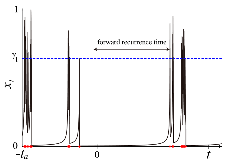
Figure 1: Schematic view of an aging process in the map (2) ($\alpha=0.8$). A trajectory is given by a solid line while renewals, $x_{t}\geq\gamma_{1}$, i.e., $\sigma(x_{t})=1$, are depicted as red crosses on time axis. $t=0$ is the time at which a measurement starts.

III Renewal processes

Renewal processes are point processes where interevent times of points are independent and identically distributed (IID) random variables Cox (1962). Therefore, renewal processes are characterized by the distribution of interevent times of renewals. Let us consider the following observation function

$$\sigma(x)=\left\{\begin{array}[]{ll}0&(x<\gamma_{1})\\ \\ 1&(x\geq\gamma_{1}),\end{array}\right.$$ (3)

where $\gamma_{1}<1$ attains $T(\gamma_{1})=1$. We call the state $\sigma=0$ the laminar phase while $\sigma=1$ the chaotic phase. In the chaotic phase, trajectories $x_{t}$ show usual chaotic behavior because of the condition (ii). Moreover, the jump transformation $T^{n(x)}$ on $x\in[\gamma_{1},1]$, which is a transformation restricted to $[\gamma_{1},1]$, has an absolutely continuous invariant probability measure whereas the original map $T$ does not, where $n(x)\equiv\min\{k\geq 1:T^{k}(x)\in[\gamma_{1},1]\}$ Thaler (1983). With the aid of these chaotic properties in the jump transformation, trajectories $\sigma_{t}=\sigma(x_{t})$ can be regarded as a renewal process because the interevent times between the events $\sigma(x_{t})=1$ are considered to be IID random variables. The probability density function (PDF) of the interevent times (or residence times of laminar phase) is given by Geisel and Thomae (1984)

$$\psi(\tau)\sim\alpha A^{\alpha}\tau^{-1-\alpha},\quad\tau\rightarrow\infty,$$ (4)

where the exponent of the PDF is controlled by the nonlinearity of the map in vicinity of the indifferent fixed point through the maps parameter $\alpha$ and $A$ is a constant, which depends on the map.

Let $N_{t}$ be the number of renewals in the time interval $(0,t)$ for a process which started on $t_{a}$, and with IID interevent times according to Eq. (4). In non-aged renewal theory $t_{a}=0$, the distribution of the number of jumps $N_{t}/t^{\alpha}$ obeys the Mittag-Leffler distribution of order $\alpha$ ($<1$) Feller (1971). Here, we review a derivation of the distribution and extend it to the aging regime Barkai and Cheng (2003). Let $S_{n}$ be the sum of the interevent times ($S_{n}=\tau_{1}+\ldots+\tau_{n}$), then we have the following relation

$$\Pr(N_{t}<n)=\Pr(S_{n}>t).$$ (5)

We notice that the interevent time PDF (4) belongs to the domain of attraction of stable laws Feller (1971). In what follows, we use the notation $\Pr_{t_{a}=0}(\cdot)$ for non-aged processes, and $\Pr(\cdot;t_{a})$ for aged processes. By the generalized central limit theorem and setting $n=t^{\alpha}x$, we have

$$\Pr_{t_{a}=0}(N_{t}/t^{\alpha}<x) = \Pr_{t_{a}=0}(S_{n}/n^{1/\alpha}>x^{-1/\alpha})$$ (6)

$$\rightarrow \int_{x^{-1/\alpha}}^{\infty}l_{\alpha}(y)dy\quad{\rm as}\quad t\rightarrow\infty,$$ (7)

where $l_{\alpha}(x)$ is the one-sided stable density with index $\alpha$, which depend on $A$ and its Laplace transform is given by

$$\int_{0}^{\infty}l_{\alpha}(x)e^{-sx}dx=\exp(-\Gamma(1-\alpha)(As)^{\alpha}).$$ (8)

In aging renewal processes, the PDF $\psi_{0}(\tau;t_{a})$ of the forward recurrence time, that is the time between the start of an observation $t=0$ and the first renewal (see Fig. 1), is different from (4). According to Barkai and Cheng (2003); Godrèche and Luck (2001), the double Laplace transform of $\psi_{0}(\tau;t_{a})$,

$$\hat{\psi}_{0}(s,s_{a})\equiv\int_{0}^{\infty}\int_{0}^{\infty}\psi_{0}(\tau,t_{a})e^{-t_{a}s_{a}-\tau s}d\tau dt_{a},$$ (9)

is given by

$$\hat{\psi}_{0}(s,s_{a})\sim\frac{s_{a}^{\alpha}-s^{\alpha}}{s_{a}^{\alpha}(s_{a}-s)}.$$ (10)

Furthermore, by Dynkin’s limit theorem Dynkin (1961), the limit PDF $(t_{a}\rightarrow\infty)$ reads

$$\psi_{0}(\tau;t_{a})\sim\frac{\sin(\pi\alpha)}{\pi}\frac{t_{a}^{\alpha}}{\tau^{\alpha}(t_{a}+\tau)}.$$ (11)

The probability of $N_{t}=0$ is given by $\int_{t}^{\infty}\psi_{0}(\tau;t_{a})d\tau$, while, for $N_{t}\geq 1$, the probability $\Pr(N_{t}<n;t_{a})$ is represented by the convolution of $\psi_{0}(\tau;t_{a})$ and $\Pr_{t_{a}=0}(N_{\tau}<n-1)$

$$\Pr(N_{t}/t^{\alpha}<x;t_{a})=1-m_{\alpha}(T_{a})$$

$$+\int_{0}^{t}\Pr_{t_{a}=0}(N_{t-\tau}<xt^{\alpha}-1)\psi_{0}(\tau;t_{a})d\tau,$$ (12)

where $m_{\alpha}(T_{a})\equiv\int_{0}^{t}\psi_{0}(\tau;t_{a})d\tau$, which is represented by the incomplete beta function,

$$m_{\alpha}(T_{a})=\frac{\sin(\pi\alpha)}{\pi}B\left(\frac{1}{T_{a}+1};1-\alpha,\alpha\right).$$ (13)

The $1-m_{\alpha}(T_{a})$ describes trajectories with no renewal events in $(0,t)$, or in the context of dynamics of maps particles which did not escape the vicinity of an unstable fixed point in the observation interval. We note that $T_{a}$ is the aging ratio, defined in introduction. In the same way as a calculation of the probability of $N_{t}/t^{\alpha}$ in non-aged renewal processes, we have

$$\Pr(N_{t}/t^{\alpha}<x;t_{a})$$ (14)

$$\cong 1-m_{\alpha}(T_{a})+\int_{0}^{t}\Pr_{t_{a}=0}\left(\frac{S_{n}}{n^{1/\alpha}}>\frac{t-\tau}{n^{1/\alpha}}\right)\psi_{0}(\tau;t_{a})d\tau$$

$$\rightarrow 1-m_{\alpha}(T_{a})+\int_{0}^{t}\psi_{0}(\tau;t_{a})\int_{\frac{t-\tau}{x^{1/\alpha}t}}^{\infty}l_{\alpha}(y)dyd\tau,$$

for $t\rightarrow\infty$. As a result, the PDF $p_{\alpha}(\xi;T_{a})$ of $\xi\equiv N_{t}/t^{\alpha}$ in the aging limit, $t_{a}/t\rightarrow T_{a}$ ($t,t_{a}\rightarrow\infty$), is written as

$$p_{\alpha}(\xi;T_{a}) = \delta(\xi)[1-m_{\alpha}(T_{a})]+\frac{\sin(\pi\alpha)}{\pi\alpha\xi^{1+1/\alpha}}$$ (15)

$$\int_{0}^{1/T_{a}}\frac{1-T_{a}y}{y^{\alpha}(1+y)}l_{\alpha}\left(\frac{1-T_{a}y}{\xi^{1/\alpha}}\right)dy.$$

This result is consistent with Schulz et al. (2012). We note that the distribution depends strongly on $T_{a}$ even when the total measurement time goes to infinity. For $T_{a}\rightarrow 0$ (non-aging limit), $p_{\alpha}(\xi;T_{a})$ converges to the Mittag-Leffler density as expected.

One can show that the mean $\langle N_{t}\rangle$ Schulz et al. (2012) is

$$\langle N_{t}\rangle=\frac{\{(t+t_{a})/A\}^{\alpha}}{\Gamma(\alpha)}B\left(\frac{1}{T_{a}+1};1,\alpha\right).$$ (16)

It will soon be usefull to define a normalized variable $\chi=N_{t}/\langle N_{t}\rangle$. Using Eq. (15) and $C_{A}\equiv t^{\alpha}/\langle N_{t}\rangle$, we have

$$P_{\alpha}(\chi;T_{a})=\frac{1}{C_{A}}p_{\alpha}(\chi/C_{A};T_{a}).$$ (17)

We note that PDF $P_{\alpha}(\chi;T_{a})$ has the advantage of being $A$ independent (PDF $p_{\alpha}(\chi;T_{a})$ depends on $A$).

IV Results

IV.1 Distributional limit theorem in the aging limit

The distributional limit theorem (14) in aging renewal processes implies that the time average of $\sigma(x_{k})$ converges in distribution:

$$\Pr\left(\frac{1}{t^{\alpha}}\sum_{k=0}^{t-1}\sigma(x_{k})<x\right) = \Pr(N_{t}/t^{\alpha}<x)$$ (18)

$$\rightarrow \int_{0}^{x}p_{\alpha}(\xi;T_{a})d\xi.$$ (19)

Because $\sigma(x)$ is an integrable function with respect to an invariant measure, this distributional limit theorem is a generalization of ADK theorem (1). By the Hopf’s ergodic theorem Hopf (1937), the ratio of the sums of arbitrary integrable observation functions $f(x)$ and $\sigma(x)$ converges to a constant for almost all initial points:

$$\frac{\sum_{k=0}^{n}f(x_{k})}{\sum_{k=0}^{n}\sigma(x_{k})}\rightarrow\frac{\int_{0}^{1}fd\mu}{\int_{0}^{1}\sigma d\mu}\quad{\rm as}\quad n\rightarrow\infty,$$ (20)

where $\mu$ is an invariant measure. Therefore, we have the following theorem. In the aging limit $t_{a}/t\rightarrow T_{a}$ as $t_{a}$ and $t\rightarrow\infty$, for all integrable functions $f(x)$ with respect to an invariant measure $\mu$, the time average of $f(x)$ converges in distribution:

$$\Pr\left(\frac{C_{f}C_{A}}{t^{\alpha}}\sum_{k=0}^{t-1}f(x_{k})<x\right)\rightarrow\int_{0}^{x}P_{\alpha}(\xi;T_{a})d\xi,$$ (21)

where $C_{f}=\int_{0}^{1}fd\mu/\mu([\gamma_{1},1])$. We note that the distribution depends on the aging ratio $T_{a}$ and $\alpha$ while we do not represent an initial density explicitly in the left-hand side in (21).

IV.2 From Dynkin’s limit theorem to evolution of density

Here, we give an explicit representation of an initial density in aging processes. In aging renewal processes, the probability that there is no renewal until time $t$ is given by $\int_{t}^{\infty}\psi_{0}(\tau;t_{a})d\tau$. Corresponding probability in the map (2) is the probability that trajectories do not escape from the interval $[0,\gamma_{1})$, which is given by $\int_{0}^{\gamma_{t}}\rho(x,t_{a})dx$, where $T^{t}(\gamma_{t})=1$ for $\gamma_{t}<1$. Using a continuous approximation, $T^{\prime}(\gamma_{t})\sim\frac{T(\gamma_{t})-T(\gamma_{t+1})}{\gamma_{t}-\gamma_{t+1}}$, near $x\cong 0$ and $T(\gamma_{t})=\gamma_{t-1}$, we have

$$\frac{\gamma_{t-1}-\gamma_{t}}{\gamma_{t}-\gamma_{t+1}}-1\sim\left(1+\frac{1}{\alpha}\right)\gamma_{t}^{1/\alpha}.$$ (22)

It follows that $\gamma_{t}\sim\alpha^{\alpha}t^{-\alpha}$ (the rigorous proof is given in Thaler (1983)). Therefore, we have the following relation:

$$\int_{0}^{\alpha^{\alpha}t^{-\alpha}}\rho(x,t_{a})dx\sim C^{\prime}\int_{t}^{\infty}\psi_{0}(\tau;t_{a})d\tau,$$ (23)

where $C^{\prime}$ is a constant independent of time. Differentiating both sides of (23) with respect to $t$ and using (11), we have

$$\rho(\alpha^{\alpha}/t^{\alpha},t_{a})\frac{\alpha^{\alpha+1}}{t^{\alpha+1}}\sim C^{\prime}\frac{\sin(\pi\alpha)}{\pi}\frac{t_{a}^{\alpha}}{t^{\alpha}(t_{a}+t)}.$$ (24)

As the result, we obtain an initial density in the aging process:

$$\rho(x,t_{a})\sim C\frac{1}{1+t_{a}x^{1/\alpha}/\alpha}.$$ (25)

The constant $C$ is the normalization constant which depends on $t_{a}$, for $t_{a}\gg 1$

$$C=\left(\int_{0}^{1}\frac{1}{1+t_{a}x^{1/\alpha}/\alpha}dx\right)^{-1}\sim\frac{\sin(\pi\alpha)}{\pi\alpha}\left(\frac{t_{a}}{\alpha}\right)^{\alpha}.$$ (26)

Surprisingly, evolutions of the density are in very good agreement with the above estimation even in small numbers of iterations and on whole space $[0,1]$ (see Fig. 2). The density cannot converge to an invariant density (equilibrium density) and will converge to the delta function $\delta(x)$ as $t_{a}$ goes to infinity. This is a direct evidence of aging in dynamical systems. We note that the scaled density converges to an infinite invariant density $\tilde{\rho}(x)$ Thaler (2000):

$$\lim_{t_{a}\rightarrow\infty}t_{a}^{1-\alpha}\rho(x,t_{a})=\tilde{\rho}(x)\sim\frac{\sin(\pi\alpha)}{\pi}\alpha^{-\alpha}x^{-1/\alpha}\quad(x\rightarrow 0)$$ (27)

Moreover, by the change of variable, $x=\alpha^{\alpha}y/t_{a}^{\alpha}$, the scaled density, $q(y)=\alpha^{\alpha}\rho(\alpha^{\alpha}y/t_{a}^{\alpha};t_{a})/t_{a}^{\alpha}$, gives a universal master curve:

$$q(y)=\frac{\sin(\pi\alpha)}{\pi\alpha}\frac{1}{1+y^{1/\alpha}}.$$ (28)

This result is consistent with a rigorous result in general intermittent maps by Thaler Thaler (2005). Figure 3 shows a convergence of the scaled density to the master curve. We note that the master curve is universal in the sense that it does not depends on details of the map except for near the fixed point $x=0$.

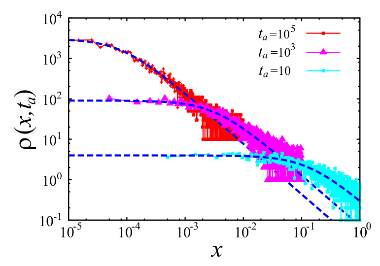
Figure 2: Initial densities for different aging times $t_{a}=10,10^{3}$ and $10^{5}$ ($\alpha=0.8$). Symbols with lines are the results of numerical simulations. Blue dashed curves are the theoretical curves without fitting parameters. For all times $t_{a}$, the densities are in a nice agreement with the theory.

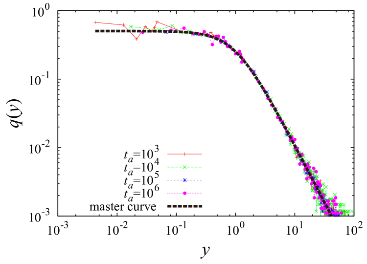
Figure 3: Scaled density ($\alpha=0.6$). Dashed line is the master curve Eq. (28) for $\alpha=0.6$. The scaled density approach to the master curve as $t_{a}\rightarrow\infty$.

IV.3 Dynamical instability

To investigate an effect of the aging on the dynamical instability, we consider the Lyapunov exponent. In general, weakly chaotic systems with infinite invariant measures have zero Lyapunov exponent Gaspard and Wang (1988); Akimoto and Aizawa (2010); Ignaccolo et al. (2001); Korabel and Barkai (2009). However, these dynamical instabilities are known as a subexponential instability quantified by the generalized Lyapunov exponent $\Lambda_{\alpha}$ Akimoto and Aizawa (2010); Korabel and Barkai (2009), which is defined as the average of the normalized Lyapunov exponent, $\Lambda_{\alpha}\equiv\langle\lambda_{\alpha}\rangle$, where $\langle\cdot\rangle$ is an average with respect to an initial density and

$$\lambda_{\alpha}\equiv\lim_{t\rightarrow\infty}\frac{1}{t^{\alpha}}\sum_{k=0}^{t-1}\ln|T^{\prime}(x_{k})|,\quad(t_{a}=0).$$ (29)

In non-aged systems, $\Lambda_{\alpha}$ does not depend on an initial density with the aid of ADK theorem. To investigate an effect of aging, we consider the generalized Lyapunov exponent in the aging limit $t_{a}/t\rightarrow T_{a}$, $\Lambda_{\alpha}(T_{a})\equiv\langle\lambda_{\alpha}(T_{a})\rangle$, where

$$\lambda_{\alpha}(T_{a})\equiv\lim_{t\rightarrow\infty}\frac{1}{t^{\alpha}}\sum_{k=0}^{t-1}\ln|T^{\prime}(x_{k})|,\quad(t_{a}/t\rightarrow T_{a}).$$ (30)

The aging generalized Lyapunov exponent is represented as

$$\Lambda_{\alpha}(T_{a})\cong\frac{1}{t^{\alpha}}\int_{0}^{t}\int_{0}^{1}g(x)\rho(x,t^{\prime}+t_{a})dxdt^{\prime},$$ (31)

where $g(x)=\ln|T^{\prime}(x)|$. Using the limit density (27), we obtain

$$\Lambda_{\alpha}(T_{a})\cong\frac{(t+t_{a})^{\alpha}-t_{a}^{\alpha}}{\alpha t^{\alpha}}\int_{0}^{1}g(x)\tilde{\rho}(x)dx.$$ (32)

for $t\gg 1$ and $t_{a}\gg 1$ with $T_{a}$ fixed. Here $\tilde{\rho}(x)=\lim_{t_{a}\to\infty}t_{a}^{1-\alpha}\rho(x,0)$ defines a unique infinite invariant density. According to ADK theorem, the non-aging generalized Lyapunov exponent ($t_{a}=0$) is given by Korabel and Barkai (2009)

$$\Lambda_{\alpha}(T_{a}=0)=\frac{1}{\alpha}\int_{0}^{1}g(x)\tilde{\rho}(x)dx.$$ (33)

In the aging limit, this relation is generalized as

$$\Lambda_{\alpha}(T_{a})=\frac{(1+T_{a})^{\alpha}-T_{a}^{\alpha}}{\alpha}\int_{0}^{1}g(x)\tilde{\rho}(x)dx.$$ (34)

This aging effect on the generalized Lyapunov exponent has been confirmed numerically (Fig. 4). The result means that the dynamical instability becomes weak as the system ages.

Using the distributional limit theorem (21), we obtain the PDF of the normalized Lyapunov exponent $\chi=\lambda_{\alpha}(T_{a})/\Lambda_{\alpha}(T_{a})$, given by PDF (17), $P_{\alpha}(\chi;T_{a})$. As shown in Fig. 5, the PDF does not depend on the total measurement time $t$ if the aging ratio $T_{a}$ is fixed, and the strength of the delta peak at $\chi=0$ is increased as the aging ratio $T_{a}$ is made larger. This delta peak corresponds to trajectories that do not escape from $[0,\gamma_{1}]$ until time $t$, which weakens the dynamical instability. These trajectories are regular rather than chaotic (not even weakly chaotic). In fact, these trajectories can be treated by a continuous approximation. For $x_{t}\cong 0$, intermittent maps we consider can be written as an ordinary differential equation Manneville (1980); Geisel and Thomae (1984):

$$\frac{dx_{t}}{dt}=a_{0}x_{t}^{1+1/\alpha}\quad(x_{t}\cong 0).$$ (35)

The solution is given by

$$x_{t}=x_{0}(1-\alpha^{-1}x_{0}^{1/\alpha}a_{0}t)^{-\alpha}$$ (36)

for $x_{t}\ll 1$ or $t\ll\alpha x_{0}^{-1/\alpha}/a_{0}$. The difference of nearby trajectories $x_{t}$ and $x^{\prime}_{t}$ such that $x_{0}$ and $x^{\prime}_{0}=x_{0}+\delta x$ ($\delta x\ll x_{0}$) is described as

$$|x_{t}-x^{\prime}_{t}|\cong\delta x(1+x_{0}^{1/\alpha}(1+\alpha^{-1})a_{0}t).$$ (37)

In the aging limit, these regular motions appear even when time $t$ goes to infinity. Therefore, in the aging dynamical systems, regular motions (RMs) and weak chaotic motions (WCMs) intrinsically coexist in the aging limit. This implies that when $t_{a}>>t$ a large fraction of particles are located close to the unstable fixed point and hence their motion is regular.

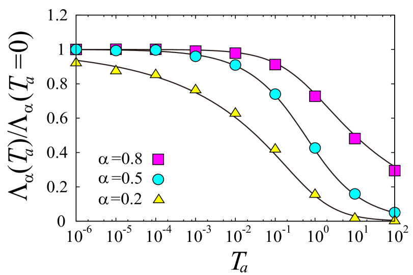
Figure 4: Generalized Lyapunov exponent as a function of the aging ratio $T_{a}$ ($\alpha=0.8$, $0.5$, and $0.2$). Different symbols are the results of numerical simulations for different $\alpha$, where the total measurement time $t$ is fixed as $10^{6}$. Curves are theoretical ones without fitting parameter ($\Lambda_{\alpha}(T_{a}=0)$ is obtained numerically). Aging strongly affects the dynamical instability when the aging time $t_{a}$ is larger than the measurement time $t$.

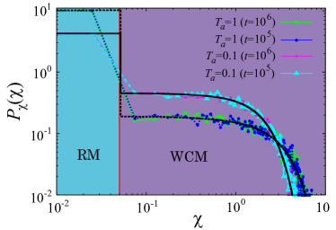
Figure 5: Probability density function $P_{\chi}({\chi})$ of the normalized Lyapunov exponent ($T_{a}=0.1$ and $1$, $t=10^{5}$ and $10^{6}$, and $\alpha=0.5$). Symbols with lines are the results of numerical simulations. Solid curves are the theoretical ones calculated by a numerical integration of the convolution in (15) using the stable density with index $1/2$, i.e., $l_{1/2}(x)=c\exp(-c^{2}/(2x))/\sqrt{2\pi x^{3}}$, where $c$ is a scaling parameter depending on $T_{a}$. Probability of regular motions is increased when the system ages. Almost all trajectories in the left-hand side of the red line exhibit regular motions (RMs) while trajectories in the right-hand side are weakly chaotic motions (WCMs), where the value of the red line ($\chi=0.05$) represents the bin size of the PDF with histogram (the bin is needed to graphically represent a delta function). Theory is in good agreement with the numerical results including the delta distribution.

V Discussion

We have shown the distribution of time averages of integrable functions in the aging limit, which is a generalization of Aaronson’s Darling-Kac theorem. Although we use intermittent maps, this generalization will be valid for all weakly chaotic maps with infinite invariant measures (more precisely, a conservative, ergodic, measure preserving transformation) because aging in dynamical systems implies that the density does not converges to an equilibrium density even when time goes to infinity (non-equilibrium non-stationary density). In fact, we have confirmed the distributional aging limit theorem in the Boole transformation Aaronson (1997).

VI Conclusion

The aging ratio $T_{a}$ plays an important role in characterizing aging systems. In the aging limit, the distribution of time-averaged observables converges to a universal distribution, which is determined by the aging ratio $T_{a}$ and the exponent $\alpha$ characterizing infinite invariant measures in dynamical systems. The mathematical basis of this universal distribution is both the generalized central limit theorem and Dynkin’s theorem for the forward recurrence time. We have also shown how to use the infinite invariant density to calculate statistical averages like the measure of separation $\Lambda_{\alpha}$ within the aging regime. From Eq. (34) we see an aged dependent pre-factor $(1+T_{a})^{\alpha}-(T_{a})^{\alpha}$ which multiplies the non-aged average. Similar averages hold for other time-averaged observables, which are integrable with respect to the infinite invariant density. Thus the infinite invariant density plays an important role for determination of ergodic properties of aging processes.

We have found that the dynamical instability is clearly divided into two different instabilities, i.e., regular motions and weakly chaotic motions, in the aging limit. Coexistence of regular and chaotic motions is reminiscent of generic Hamiltonian systems. However, the meaning of the coexistence is completely different. In aging dynamical systems, the probability of finding regular motions is increased according to the aging ratio $T_{a}$, whereas regular and chaotic phase spaces do not depend on $T_{a}$ in generic Hamiltonian systems.