Distribution function of the endpoint fluctuations of one-dimensional directed polymers in a random potential

Abstract

The explicit expression for the the probability distribution function of the endpoint fluctuations of one-dimensional directed polymers in random potential is derived in terms of the Bethe ansatz replica technique by mapping the replicated problem to the $N$-particle quantum boson system with attractive interactions.

I Introduction

One-dimensional directed polymers in a quenched random potential and equivalent problem of the solutions of the KPZ-equation KPZ describing the growth in time of an interface in the presence of noise have been the subject of intense investigations during the past two decades (see e.g. hh_zhang_95 ; burgers_74 ; kardar_book ; hhf_85 ; numer1 ; numer2 ; kardar_87 ; bouchaud-orland ; Brunet-Derrida ; Johansson ; Prahofer-Spohn ; Ferrari-Spohn1 ; Corwin ). The model of directed polymers describes an elastic string directed along the $\tau$-axis within an interval $[0,t]$. Randomness enters the problem through a disorder potential $V[\phi(\tau),\tau]$, which competes against the elastic energy. The system is defined by the Hamiltonian

$$H[\phi(\tau),V]=\int_{0}^{t}d\tau\Bigl{\{}\frac{1}{2}\bigl{[}\partial_{\tau}\phi(\tau)\bigr{]}^{2}+V[\phi(\tau),\tau]\Bigr{\}};$$ (1)

where the disorder potential $V[\phi,\tau]$ is Gaussian distributed with a zero mean $\overline{V(\phi,\tau)}=0$ and the $\delta$-correlations:

$${\overline{V(\phi,\tau)V(\phi^{\prime},\tau^{\prime})}}=u\delta(\tau-\tau^{\prime})\delta(\phi-\phi^{\prime})$$ (2)

Here the parameter $u$ describes the strength of the disorder.

In what follows we consider the problem in which the polymer is fixed at the origin, $\phi(0)=0$ and it is free at $\tau=t$. In other words, for a given realization of the random potential $V$ the partition function of the considered system is:

$$Z=\int_{-\infty}^{+\infty}dx\;Z(x)\;=\;\exp\{-\beta F\}$$ (3)

where

$$Z(x)=\int_{\phi(0)=0}^{\phi(t)=x}{\cal D}\phi(\tau)\;\mbox{\Large e}^{-\beta H[\phi]}$$ (4)

is the partition function of the system with the fixed boundary condition, $\phi(t)=x$ and $F$ is the total free energy. Besides the usual extensive part $f_{0}t$ (where $f_{0}$ is the linear free energy density), the total free energy $F$ of such system is known to contain the disorder dependent fluctuating contribution which in the limit of large $t$ scales as $t^{1/3}$ (see e.g. hhf_85 ; numer1 ; numer2 ; kardar_87 ). In other words, in the limit of large $t$ the total (random) free energy of the system can be represented as $F=f_{0}t+ct^{1/3}f$, where $c$ is a non-universal parameter, which depends on the temperature and the strength of disorder, and $f$ is the random quantity which in the thermodynamic limit $t\to\infty$ is described by a non-trivial universal distribution function $P(f)$. The trivial self-averaging contribution $f_{0}t$ to the free energy can be eliminated from the further study by the simple redefinition of the partition function, $Z=\exp\{-\beta f_{0}t\}\,\tilde{Z}$, so that $\tilde{Z}=\exp\{-\lambda f\}$, where $\lambda=\beta\,c\,t^{1/3}$. Thus, to simplify notations the contribution $f_{0}t$ will be just dropped out in the further calculations.

For the problem with the zero boundary conditions, $\phi(0)=\phi(t)=0$, the distribution function $P(f)$ was demonstrated to be described by the Gaussian Unitary Ensemble (GUE) Tracy-Widom distribution KPZ-TW1 ; KPZ-TW2 ; BA-replicas ; LeDoussal1 . On the other hand, the free energy distribution function of the directed polymers with the free boundary conditions, eqs.(1)-(4), was shown to be given by the Gaussian Orthogonal Ensemble (GOE) Tracy-Widom distribution LeDoussal2 ; goe In the course of these derivations rather efficient Bethe ansatz replica technique has been developed BA-replicas ; LeDoussal1 ; LeDoussal2 ; goe . Here in terms of this technique we are going to study on the statistical properties of the transverse fluctuations of the directed polymers. The scaling properties of the typical value of the endpoint deviations, $\phi(t)$, at large times is well known: $\overline{\langle\phi(t)\rangle^{2}}\;\propto\;t^{4/3}\;\;$ (here $\langle...\rangle$ denotes the thermal average and $\overline{(...)}$ is the average over the disorder potential, eq.(2)) hhf_85 ; numer1 ; numer2 ; kardar_87 . Much more interesting object is the probability distribution function $P(x)$ for the rescaled quantity $x=\phi(t)/t^{2/3}$ which is expected to become a universal function in the limit $t\to\infty$. Recently this function has been derived in terms of the so called maximal point of the $\mbox{Airy}_{2}$ process minus a parabola math1 ; math2 ; math3 , which is believed to descibe the scaling limit of the endpoint of the directed polymers in a random potential. The long-standing conjecture that the top line of the Airy line ensemble minus a parabola attains its maximum at a unique point was recently proved in Corwin-Hammond . The obtained explicit expression for $P(x)$ turned out to be rather complicated and its analytic properties is not so easy to analyze although the asymptotic behavior of this function is already known: $P(x\to\infty)\sim\exp\{-|x|^{3}/12\}$math2 .

In this work the explicit form of the distribution function of the directed polymer’s endpoint fluctuations will be derived in terms of the Bethe ansatz replica technique. The distribution function we are going to consider is defined as follows:

$$W(x)\;=\;\lim_{t\to\infty}\;\mbox{Prob}\bigl{[}\phi(t)t^{-2/3}\;>\;x\bigr{]}\;=\;\int_{x}^{\infty}\;dx^{\prime}\;P(x^{\prime})$$ (5)

This function gives the probability that the rescaled value of the polymer’s right endpoint $\phi(t)/t^{2/3}$ is bigger than a given value $x$. In this paper it will be shown that (see eqs.(79)-(84) below)

$$W(x)\;=\;\int_{-\infty}^{+\infty}df\;F_{1}(-f)\int_{0}^{+\infty}d\omega\int_{0}^{+\infty}d\omega^{\prime}\bigl{(}\hat{1}-\hat{B}_{-f}\bigr{)}^{-1}(\omega,\omega^{\prime})\;\Phi(\omega^{\prime},\omega;\;f,x)$$ (6)

Here $\hat{B}_{-f}$ is the integral operator with the kernel $B_{-f}(\omega,\omega^{\prime})=\operatorname{Ai}(\omega+\omega^{\prime}-f)\;\;(\omega,\omega^{\prime}\,>\,0)$, the function $F_{1}(-f)=\det\bigl{[}\hat{1}-\hat{B}_{-f}\bigr{]}$ is the GOE Tracy-Widom distribution and $\bigl{(}\hat{1}-\hat{B}_{-f}\bigr{)}^{-1}(\omega,\omega^{\prime})$ denotes the kernel of the inverse operator $\bigl{(}\hat{1}-\hat{B}_{-f}\bigr{)}^{-1}$ in $\omega$ and $\omega^{\prime}$ (note that since $F_{1}(-f)>0$ for all real $f$, the operator $\bigl{(}\hat{1}-\hat{B}_{-f}\bigr{)}$ is invertible). The function $\Phi(\omega^{\prime},\omega;\;f,x)$ is defined as follows:

$$\Phi(\omega,\omega^{\prime};\;f,x)=-\frac{1}{2}\int_{0}^{+\infty}dy\; \Biggl{[} \Bigl{(}\frac{\partial}{\partial\omega}-\frac{\partial}{\partial\omega^{\prime}}\Bigr{)}\Psi\bigl{(}\omega-\frac{1}{2}f+y;\;x\bigr{)}\Psi\bigl{(}\omega^{\prime}-\frac{1}{2}f+y;\;-x\bigr{)}+$$ (7)

$$+ \Bigl{(}\frac{\partial}{\partial\omega}+\frac{\partial}{\partial\omega^{\prime}}\Bigr{)}\Psi\bigl{(}\omega-\frac{1}{2}f-y;\;x\bigr{)}\Psi\bigl{(}\omega^{\prime}-\frac{1}{2}f+y;\;-x\bigr{)}\Biggr{]}$$

where

$$\Psi(\omega;x)\;=\;2^{1/3}\mbox{Ai}\Bigl{[}2^{1/3}\bigl{(}\omega+\frac{1}{8}x^{2}\bigr{)}\Bigr{]}\,\exp\bigl{\{}-\frac{1}{2}\omega x\bigr{\}}$$ (8)

The above result looks quite similar to the one obtained in math1 , although at the moment I am not able to provide the proof that these results are indeed the same¹. In any case, the above expressions, eqs.(6)-(8), for the probability function $P(x)$ look as complicated as the ones obtained in Refs.math1 ; math2 ; math3 , and for the moment its analytic properties are not clear.

The paper is organized as follows. In Section II we define the distribution function $W(x)$ via the two-point free energy distribution function $V_{x}(f_{1},f_{2})$ which give the probability that the free energy of the polymer with the endpoint located above a position $x$ is bigger than a given value $f_{1}$, while the free energy of the polymer with the endpoint located below the position $x$ is bigger than a given value $f_{2}$. In Section III the function $V_{x}(f_{1},f_{2})$ is defined by mapping the considered problem to the one-dimensional $N$-particle system of quantum bosons with attractive $\delta$-interactions. In Section IV the explicit expression for the probability function $V_{x}(f_{1},f_{2})$ is obtained in terms of the Bethe ansatz replica technique. Finally, in Section V the result eqs.(6)-(8) is derived. Conclusions and future perspectives are discussed in Section VI.

II The endpoint probability distribution function

In terms of the partition function $Z(x)$, eqs.(4), the probability distribution function of the polymer’s endpoint $W(x)$, eq.(5), can be defined as follows:

$$W(x) = \lim_{t\to\infty}\;\overline{\Biggl{(}\int_{x}^{+\infty}dx^{\prime}\frac{Z(x^{\prime})}{\int_{-\infty}^{+\infty}dx^{\prime}\;Z(x^{\prime})}\Biggr{)}}$$ (9)

$$= \lim_{t\to\infty}\;\overline{\Biggl{(}\frac{Z^{(+)}(x)}{Z^{(+)}(x)+Z^{(-)}(x)}\Biggr{)}}$$

where

$$Z^{(-)}(x) \equiv \int_{-\infty}^{x}dx^{\prime}\;Z(x^{\prime})\;=\;\exp\{-\lambda f_{(-)}\}$$ (10)

$$Z^{(+)}(x) \equiv \int_{x}^{+\infty}dx^{\prime}\;Z(x^{\prime})\;=\;\exp\{-\lambda f_{(+)}\}$$ (11)

where the parameter $\lambda\propto t^{1/3}$ and $f_{(\pm)}$ are the free energies of the polymers with the endpoint $\phi(t)$ located correspondingly above and below a given position $x$. According to these definitions we find

$$W(x)\;=\;\lim_{\lambda\to\infty}\;\frac{\exp\{-\lambda f_{(+)}\}}{\exp\{-\lambda f_{(-)}\}\,+\,\exp\{-\lambda f_{(+)}\}}\;=\;\left\{\begin{array}[]{ll}0,\;\;\;\;\mbox{for}\;\;f_{(-)}<f_{(+)}\\ \\ 1,\;\;\;\;\mbox{for}\;\;f_{(-)}>f_{(+)}\end{array}\right.$$ (12)

Let us introduce the joint probability density function ${\cal P}_{x}\bigl{[}f_{(+)};f_{(-)}\bigr{]}$. By definition the quantity ${\cal P}_{x}\bigl{[}f_{(+)};f_{(-)}\bigr{]}\,df_{(+)}\,df_{(-)}$ gives the probability that the free energy of the polymer with the endpoint located below $x$ is equal to $f_{(-)}$ (within the interval $df_{(-)}$), while the free energy of the polymer with the endpoint located above $x$ is equal to $f_{(+)}$ (within the interval $df_{(+)}$). Thus, according to eq.(12),

$$W(x)\;=\;\int_{-\infty}^{+\infty}df_{(+)}\int_{f_{(+)}}^{+\infty}df_{(-)}{\cal P}_{x}\bigl{[}f_{(+)};f_{(-)}\bigr{]}$$ (13)

Let us introduce one more joint probability distribution function:

$$V_{x}(f_{1},f_{2})\;=\;\mbox{Prob}\bigl{[}f_{(+)}>f_{1};\;f_{(-)}>f_{2}\bigr{]}\;=\;\int_{f_{1}}^{+\infty}df_{(+)}\int_{f_{2}}^{+\infty}df_{(-)}\,{\cal P}_{x}\bigl{[}f_{(+)};f_{(-)}\bigr{]}$$ (14)

This two-point free energy distribution function gives the probability that the free energy of the polymer with the endpoint located above the position $x$ is bigger than a given value $f_{1}$, while the free energy of the polymer with the endpoint located below the position $x$ is bigger than a given value $f_{2}$. According to this definition,

$${\cal P}_{x}\bigl{[}f_{1};f_{2}\bigr{]}\;=\;\frac{\partial}{\partial f_{1}}\,\frac{\partial}{\partial f_{2}}\,V_{x}(f_{1},f_{2})$$ (15)

Substituting this relation into eq.(13) we find

$$W(x)\;=\;\int_{-\infty}^{+\infty}df_{1}\int_{f_{1}}^{+\infty}df_{2}\frac{\partial}{\partial f_{1}}\,\frac{\partial}{\partial f_{2}}\,V_{x}(f_{1},f_{2})$$ (16)

Integrating by parts over $f_{2}$ and taking into account that $V_{x}(f_{1},f_{2})\big{|}_{f_{2}=+\infty}=0$ we get

$$W(x)\;=\;-\int_{-\infty}^{+\infty}df_{1}\Bigl{(}\frac{\partial}{\partial f_{1}}\,V_{x}(f_{1},f_{2})\Bigr{)}\Big{|}_{f_{2}=f_{1}+0}$$ (17)

Thus, to get the distribution function $W(x)$ for the polymer’s endpoint fluctuations we have to derive the two-point free energy distribution function $V_{x}(f_{1},f_{2})$ first. Note that this function is different from the two-point free energy distribution function derived in Prolhac-Spohn which describes joint statistics of the free energies of the directed polymers coming to two different endpoints.

III Mapping to quantum bosons

According to the definition, eq.(14), the probability distribution function $V_{x}(f_{1},f_{2})$ can be defined as follows:

$$V_{x}(f_{1},f_{2})=\lim_{\lambda\to\infty}\sum_{L=0}^{\infty}\sum_{R=0}^{\infty}\frac{(-1)^{L}}{L!}\frac{(-1)^{R}}{R!}\exp\bigl{(}\lambda Lf_{1}+\lambda Rf_{2}\bigr{)}\;\overline{\bigl{[}Z^{(+)}(x)\bigr{]}^{L}\,\bigl{[}Z^{(-)}(x)\bigr{]}^{R}}$$ (18)

Indeed, substituting here the definitions, eqs.(10)-(11), we find:

$$V_{x}(f_{1},f_{2}) = \lim_{\lambda\to\infty}\int_{-\infty}^{+\infty}df_{(+)}\int_{-\infty}^{+\infty}df_{(-)}{\cal P}_{x}\bigl{[}f_{(+)};f_{(-)}\bigr{]}\sum_{L=0}^{\infty}\sum_{R=0}^{\infty}\frac{(-1)^{L}}{L!}\frac{(-1)^{R}}{R!}\,\exp\bigl{[}\lambda L(f_{1}-f_{(+)})\bigr{]}\,\exp\bigl{[}\lambda R(f_{2}-f_{(-)})\bigr{]}$$ (19)

$$= \lim_{\lambda\to\infty}\int_{-\infty}^{+\infty}df_{(+)}\int_{-\infty}^{+\infty}df_{(-)}{\cal P}_{x}\bigl{[}f_{(+)};f_{(-)}\bigr{]}\exp\Bigl{[}-\mbox{\Large e}^{\lambda(f_{1}-f_{(+)})}\,-\mbox{\Large e}^{\lambda(f_{2}-f_{(-)})}\Bigr{]}$$

$$= \int_{-\infty}^{+\infty}df_{(+)}\int_{-\infty}^{+\infty}df_{(-)}{\cal P}_{x}\bigl{[}f_{(+)};f_{(-)}\bigr{]}\theta\bigl{(}f_{(+)}-f_{1}\bigr{)}\,\theta\bigl{(}f_{(-)}-f_{2}\bigr{)}$$

where $\theta(f)$ is the Heaviside step function. We see that the above representation coincides with the definition, eq.(14).

Further calculations of the two-point distribution function $V_{x}(f_{1},f_{2})$ to a large extent repeats the procedure described in detail in the previous paper goe for the one-point free energy distribution function. Using the definitions, eqs.(10)-(11), the distribution function, eq.(18), can be represented as follows:

$$V_{x}(f_{1},f_{2})=\lim_{\lambda\to\infty}\sum_{L,R=0}^{\infty}\frac{(-1)^{L+R}}{L!R!}\exp\bigl{(}\lambda Lf_{1}+\lambda Rf_{2}\bigr{)}\;\int_{-\infty}^{x}dx_{1}...dx_{L}\int_{x}^{+\infty}dy_{1}...dy_{R}\Psi(x_{1},...,x_{L},y_{R},...,y_{1};t)$$ (20)

where

$$\Psi(x_{1},...,x_{N};t)\;\equiv\;\overline{Z(x_{1})\,Z(x_{2})\,...\,Z(x_{N})}=\prod_{a=1}^{N}\Biggl{[}\int_{\phi_{a}(0)=0}^{\phi_{a}(t)=x_{a}}{\cal D}\phi_{a}(\tau)\Biggr{]}\;\exp\bigl{(}-\beta H_{N}[\phi_{1},\phi_{2},...,\phi_{N}]\bigr{)}$$ (21)

with the replica Hamiltonian

$$H_{N}[\phi_{1},\phi_{2},...,\phi_{N}]\;=\;\frac{1}{2}\int_{0}^{t}d\tau\Biggl{(}\sum_{a=1}^{N}\bigl{[}\partial_{\tau}\phi_{a}(\tau)\bigr{]}^{2}-\beta u\sum_{a\not=b}^{N}\delta\bigl{[}\phi_{a}(\tau)-\phi_{b}(\tau)\bigr{]}\Biggr{)}$$ (22)

The propagator $\Psi({\bf x};t)$, eq.(21), describes $N$ trajectories $\phi_{a}(\tau)$ all starting at zero ($\phi_{a}(0)=0$), and coming to $N$ different points $\{x_{1},...,x_{N}\}$ at $\tau=t$. One can easily show that $\Psi({\bf x};t)$ can be obtained as the solution of the the imaginary-time Schrödinger equation

$$-\beta\,\partial_{t}\Psi({\bf x};t)=\hat{H}\Psi({\bf x};t)$$ (23)

with the initial condition

$$\Psi({\bf x};0)=\Pi_{a=1}^{N}\delta(x_{a})$$ (24)

Here the Hamiltonian is

$$\hat{H}=-\frac{1}{2}\sum_{a=1}^{N}\partial_{x_{a}}^{2}-\frac{1}{2}\,\kappa\sum_{a\not=b}^{N}\delta(x_{a}-x_{b})$$ (25)

and the interaction parameter $\kappa=\beta^{3}u$. This Hamiltonian describes $N$ bose-particles interacting via the attractive two-body potential $-\kappa\delta(x)$.

A generic eigenstate of such system is characterized by $N$ momenta $\{q_{a}\}\;(a=1,...,N)$ which are splitted into $M$ ($1\leq M\leq N$) ”clusters” described by continuous real momenta $q_{\alpha}$ $(\alpha=1,...,M)$ and having $n_{\alpha}$ discrete imaginary ”components” (for details see Lieb-Liniger ; McGuire ; Yang ; Calabrese ; BA-replicas ; rev-TW ):

$$q_{a}\;\equiv\;q^{\alpha}_{r}\;=\;q_{\alpha}-\frac{i\kappa}{2}(n_{\alpha}+1-2r)\;\;;\;\;\;\;\;\;\;\;\;\;(r=1,...,n_{\alpha})$$ (26)

with the global constraint

$$\sum_{\alpha=1}^{M}n_{\alpha}=N$$ (27)

A generic solution $\Psi({\bf x},t)$ of the Schrödinger equation (23) with the initial conditions, eq.(24), can be represented in the form of the linear combination of the eigenfunctions $\Psi_{\bf q}^{(M)}({\bf x})$:

$$\Psi(x_{1},...,x_{N};t)=\sum_{M=1}^{N}\frac{1}{M!}\Biggl{[}\int{\cal D}^{(M)}({\bf q},{\bf n})\Biggr{]}\;|C_{M}({\bf q},{\bf n})|^{2}\;\Psi^{(M)}_{{\bf q}}({\bf x}){\Psi^{(M)}_{{\bf q}}}^{*}({\bf 0})\;\exp\bigl{\{}-E_{M}({\bf q},{\bf n})t\bigr{\}}$$ (28)

where we have introduced the notation

$$\int{\cal D}^{(M)}({\bf q},{\bf n})\equiv\prod_{\alpha=1}^{M}\Biggl{[}\int_{-\infty}^{+\infty}\frac{dq_{\alpha}}{2\pi}\sum_{n_{\alpha}=1}^{\infty}\Biggr{]}{\boldsymbol{\delta}}\Bigl{(}\sum_{\alpha=1}^{M}n_{\alpha}\;,\;N\Bigr{)}$$ (29)

and ${\boldsymbol{\delta}}(k,m)$ is the Kronecker symbol; note that the presence of this Kronecker symbol in the above equation allows to extend the summations over $n_{\alpha}$’s to infinity. Here (non-normalized) eigenfunctions are BA-replicas ; rev-TW

$$\Psi^{(M)}_{{\bf q}}({\bf x})=\sum_{{\cal P}}\;\prod_{a<b}^{N}\Biggl{[}1+i\kappa\frac{\operatorname{sgn}(x_{a}-x_{b})}{q_{{\cal P}_{a}}-q_{{\cal P}_{b}}}\Biggr{]}\;\exp\Bigl{[}i\sum_{a=1}^{N}q_{{\cal P}_{a}}x_{a}\Bigr{]}$$ (30)

where the summation goes over $N!$ permutations ${\cal P}$ of $N$ momenta $q_{a}$, eq.(26), over $N$ particles $x_{a}$; the normalization factor

$$|C_{M}({\bf q},{\bf n})|^{2}=\frac{\kappa^{N}}{N!\prod_{\alpha=1}^{M}\bigl{(}\kappa n_{\alpha}\bigr{)}}\prod_{\alpha<\beta}^{M}\frac{\big{|}q_{\alpha}-q_{\beta}-\frac{i\kappa}{2}(n_{\alpha}-n_{\beta})\big{|}^{2}}{\big{|}q_{\alpha}-q_{\beta}-\frac{i\kappa}{2}(n_{\alpha}+n_{\beta})\big{|}^{2}}$$ (31)

and the eigenvalues:

$$E_{M}({\bf q},{\bf n})\;=\;\frac{1}{2\beta}\sum_{\alpha=1}^{N}q_{a}^{2} = \frac{1}{2\beta}\sum_{\alpha=1}^{M}\;n_{\alpha}q_{\alpha}^{2}-\frac{\kappa^{2}}{24\beta}\sum_{\alpha=1}^{M}(n_{\alpha}^{3}-n_{\alpha})$$ (32)

$$= \sum_{\alpha=1}^{M}\Bigl{[}\frac{1}{2\beta}n_{\alpha}q_{\alpha}^{2}-\frac{\kappa^{2}}{24\beta}n_{\alpha}^{3}\Bigr{]}+\frac{\kappa^{2}}{24\beta}N$$

The last term in the above expression provides just the trivial contribution to the selfaveraging part of the free energy (discussed in the Introduction) and therefore it will be dropped out of the further calculations.

Using the definition, eq.(30), one can easily prove that

$$\Psi^{(M)}_{{\bf q}}({\bf 0})=N!$$ (33)

In this way the problem of the calculation of the probability distribution function, eq.(20), reduces to the summation over all the spectrum of the eigenstates of the $N$-particle bosonic problem, which is parametrized by the set of both continuous, $\{q_{1},...,q_{M}\}$, and discrete $\{n_{1},...,n_{M}\};\;(M=1,...,N);\;(N=1,...,\infty)$ degrees of freedom.

IV Two-point free energy distribution function

Substituting eqs.(28)-(33) into eq.(20), we get:

$$V_{x}(f_{1},f_{2}) = 1+\lim_{\lambda\to\infty}\sum_{L+R\geq 1}^{\infty}\;(-1)^{L+R}\;\mbox{\LARGE e}^{\lambda Lf_{1}+\lambda Rf_{2}}\times$$

$$\times \sum_{M=1}^{L+R}\frac{1}{M!}\prod_{\alpha=1}^{M}\Biggl{[}\sum_{n_{\alpha}=1}^{\infty}\int_{-\infty}^{+\infty}\frac{dq_{\alpha}}{2\pi\kappa n_{\alpha}}\kappa^{n_{\alpha}}\mbox{\LARGE e}^{-\frac{t}{2\beta}n_{\alpha}q_{\alpha}^{2}+\frac{\kappa^{2}t}{24\beta}n_{\alpha}^{3}}\Biggr{]}\;{\boldsymbol{\delta}}\Bigl{(}\sum_{\alpha=1}^{M}n_{\alpha}\;,\;L+R\Bigr{)}\;|\tilde{C}_{M}({\bf q},{\bf n})|^{2}\;I_{L,R}({\bf q},{\bf n})$$

where

$$|\tilde{C}_{M}({\bf q},{\bf n})|^{2}\;=\;\prod_{\alpha<\beta}^{M}\frac{\big{|}q_{\alpha}-q_{\beta}-\frac{i\kappa}{2}(n_{\alpha}-n_{\beta})\big{|}^{2}}{\big{|}q_{\alpha}-q_{\beta}-\frac{i\kappa}{2}(n_{\alpha}+n_{\beta})\big{|}^{2}}$$ (35)

and

$$I_{L,R}({\bf q},{\bf n}) = \sum_{{\cal P}^{(L,R)}}\sum_{{\cal P}^{(L)}}\sum_{{\cal P}^{(R)}}\;\prod_{a=1}^{L}\prod_{c=1}^{R}\Biggl{[}\frac{q_{{\cal P}_{a}^{(L)}}-q_{{\cal P}_{c}^{(R)}}-i\kappa}{q_{{\cal P}_{a}^{(L)}}-q_{{\cal P}_{c}^{(R)}}}\Biggr{]}\times\prod_{a<b}^{L}\Biggl{[}\frac{q_{{\cal P}_{a}^{(L)}}-q_{{\cal P}_{b}^{(L)}}-i\kappa}{q_{{\cal P}_{a}^{(L)}}-q_{{\cal P}_{b}^{(L)}}}\Biggr{]}\times\prod_{c<d}^{R}\Biggl{[}\frac{q_{{\cal P}_{c}^{(R)}}-q_{{\cal P}_{d}^{(R)}}+i\kappa}{q_{{\cal P}_{c}^{(R)}}-q_{{\cal P}_{d}^{(R)}}}\Biggr{]}\times$$ (36)

$$\times \int_{-\infty<x_{1}\leq...\leq x_{L}\leq x}dx_{1}...dx_{L}\;\exp\Bigl{[}i\sum_{a=1}^{L}(q_{{\cal P}_{a}^{(L)}}-i\epsilon)x_{a}\Bigr{]}$$

$$\times \int_{x\leq y_{R}\leq...\leq y_{1}<+\infty}dy_{R}...dy_{1}\;\exp\Bigl{[}i\sum_{c=1}^{R}(q_{{\cal P}_{c}^{(R)}}+i\epsilon)y_{c}\Bigr{]}$$

Here the summation over all permutations ${\cal P}$ of $(L+R)$ momenta $\{q_{1},...,q_{L+R}\}$ over $L$ ”left” particles $\{x_{1},...,x_{L}\}$ and $R$ ”right” particles $\{y_{R},...,y_{1}\}$ are divided into three parts: the permutations ${\cal P}^{(L)}$ of $L$ momenta (taken at random out of the total list $\{q_{1},...,q_{L+R}\}$) over $L$ ”left” particles, the permutations ${\cal P}^{(R)}$ of the remaining $R$ momenta over $R$ ”right” particles, and finally the permutations ${\cal P}^{(L,R)}$ (or the exchange) of the momenta between the group $"L"$ and the group $"R"$. Note also that the integrations both over $x_{a}$’s and over $y_{c}$’s in eq.(36) require proper regularization at $-\infty$ and $+\infty$ correspondingly. This is done in the standard way by introducing a supplementary parameter $\epsilon$ which will be set to zero in final results. The result of the integrations can be represented as follows:

$$I_{L,R}({\bf q},{\bf n}) = i^{-(L+R)}\;\exp\bigl{\{}ix\sum_{\alpha=1}^{M}n_{\alpha}q_{\alpha}\bigr{\}}\sum_{{\cal P}^{(L,R)}}\;\;\prod_{a=1}^{L}\prod_{c=1}^{R}\Biggl{[}\frac{q_{{\cal P}_{a}^{(L)}}-q_{{\cal P}_{c}^{(R)}}-i\kappa}{q_{{\cal P}_{a}^{(L)}}-q_{{\cal P}_{c}^{(R)}}}\Biggr{]}\times$$ (37)

$$\times \sum_{{\cal P}^{(L)}}\;\;\frac{1}{q^{(-)}_{{\cal P}_{1}^{(L)}}\bigl{(}q^{(-)}_{{\cal P}_{1}^{(L)}}+q^{(-)}_{{\cal P}_{2}^{(L)}}\bigr{)}...\bigl{(}q^{(-)}_{{\cal P}_{1}^{(L)}}+...+q^{(-)}_{{\cal P}_{L}^{(L)}}\bigr{)}}\prod_{a<b}^{L}\Biggl{[}\frac{q^{(-)}_{{\cal P}_{a}^{(L)}}-q^{(-)}_{{\cal P}_{b}^{(L)}}-i\kappa}{q^{(-)}_{{\cal P}_{a}^{(L)}}-q^{(-)}_{{\cal P}_{b}^{(L)}}}\Biggr{]}\times$$

$$\times \sum_{{\cal P}^{(R)}}\;\;\frac{(-1)^{R}}{q^{(+)}_{{\cal P}_{1}^{(R)}}\bigl{(}q^{(+)}_{{\cal P}_{1}^{(R)}}+q^{(+)}_{{\cal P}_{2}^{(R)}}\bigr{)}...\bigl{(}q^{(+)}_{{\cal P}_{1}^{(R)}}+...+q^{(+)}_{{\cal P}_{R}^{(R)}}\bigr{)}}\prod_{c<d}^{R}\Biggl{[}\frac{q^{(+)}_{{\cal P}_{c}^{(R)}}-q^{(+)}_{{\cal P}_{d}^{(R)}}+i\kappa}{q^{(+)}_{{\cal P}_{c}^{(R)}}-q^{(+)}_{{\cal P}_{d}^{(R)}}}\Biggr{]}$$

where

$$q^{(\pm)}_{a}\;\equiv\;q_{a}\pm i\epsilon$$ (38)

and where we have used the fact that for any permutation of the momenta, eq.(26), one has:

$$\sum_{a=1}^{L+R}q_{{\cal P}_{a}}\;=\;\sum_{\alpha=1}^{M}n_{\alpha}q_{\alpha}$$ (39)

Using the Bethe ansatz combinatorial identity LeDoussal2 ,

$$\sum_{P}\frac{1}{q_{p_{1}}(q_{p_{1}}+q_{p_{2}})...(q_{p_{1}}+...+q_{p_{N}})}\prod_{a<b}^{N}\Biggl{[}\frac{q_{p_{a}}-q_{p_{b}}-i\kappa}{q_{p_{a}}-q_{p_{b}}}\Biggr{]}\;=\;\frac{1}{\prod_{a=1}^{N}q_{a}}\;\prod_{a<b}^{N}\Biggl{[}\frac{q_{a}+q_{b}+i\kappa}{q_{a}+q_{b}}\Biggr{]}$$ (40)

(where the summation goes over all permutations $P$ of $N$ momenta $\{q_{1},...,q_{N}\}$) we get:

$$I_{L,R}({\bf q},{\bf n}) = i^{-(L+R)}\;\exp\bigl{\{}ix\sum_{\alpha=1}^{M}n_{\alpha}q_{\alpha}\bigr{\}}\sum_{{\cal P}^{(L,R)}}\;\;\prod_{a=1}^{L}\prod_{c=1}^{R}\Biggl{[}\frac{q_{{\cal P}_{a}^{(L)}}-q_{{\cal P}_{c}^{(R)}}-i\kappa}{q_{{\cal P}_{a}^{(L)}}-q_{{\cal P}_{c}^{(R)}}}\Biggr{]}\times$$ (41)

$$\times \frac{1}{\prod_{a=1}^{L}q^{(-)}_{{\cal P}_{a}^{(L)}}}\prod_{a<b}^{L}\Biggl{[}\frac{q^{(-)}_{{\cal P}_{a}^{(L)}}+q^{(-)}_{{\cal P}_{b}^{(L)}}+i\kappa}{q^{(-)}_{{\cal P}_{a}^{(L)}}+q^{(-)}_{{\cal P}_{b}^{(L)}}}\Biggr{]}\times\frac{(-1)^{R}}{\prod_{c=1}^{R}q^{(+)}_{{\cal P}_{c}^{(R)}}}\prod_{c<d}^{R}\Biggl{[}\frac{q^{(+)}_{{\cal P}_{c}^{(R)}}+q^{(+)}_{{\cal P}_{d}^{(R)}}-i\kappa}{q^{(+)}_{{\cal P}_{c}^{(R)}}+q^{(+)}_{{\cal P}_{d}^{(R)}}}\Biggr{]}$$

Further simplification comes from the following important property of the Bethe ansatz wave function, eq.(30). It has such structure that for ordered particles positions (e.g. $x_{1}<x_{2}<...<x_{N}$) in the summation over permutations the momenta $q_{a}$ belonging to the same cluster also remain ordered. In other words, if we consider the momenta, eq.(26), of a cluster $\alpha$, $\{q_{1}^{\alpha},q_{2}^{\alpha},...,q_{n_{\alpha}}^{\alpha}\}$, belonging correspondingly to the particles $\{x_{i_{1}}<x_{i_{2}}<...<x_{i_{n_{\alpha}}}\}$, the permutation of any two momenta $q_{r}^{\alpha}$ and $q_{r^{\prime}}^{\alpha}$ of this ordered set gives zero contribution. Thus, in order to perform the summation over the permutations ${\cal P}^{(L,R)}$ in eq.(41) it is sufficient to split the momenta of each cluster into two parts: $\{q_{1}^{\alpha},...,q_{m_{\alpha}}^{\alpha}||q_{m_{\alpha}+1}^{\alpha}...,q_{n_{\alpha}}^{\alpha}\}$, where $m_{\alpha}=0,1,...,n_{\alpha}$ and where the momenta $q_{1}^{\alpha},...,q_{m_{\alpha}}^{\alpha}$ belong to the particles of the sector $"L"$, while the momenta $q_{m_{\alpha}+1}^{\alpha}...,q_{n_{\alpha}}^{\alpha}$ belong to the particles of the sector $"R"$.

Let us introduce the numbering of the momenta of the sector $"R"$ in the reversed order:

$$q_{n_{\alpha}}^{\alpha} \to {q^{*}}_{1}^{\alpha}$$

$$q_{n_{\alpha}-1}^{\alpha} \to {q^{*}}_{2}^{\alpha}$$

$$........$$

$$q_{m_{\alpha}+1}^{\alpha} \to {q^{*}}_{s_{\alpha}}^{\alpha}$$ (42)

where $m_{\alpha}+s_{\alpha}=n_{\alpha}$ and (s.f. eq.(26))

$${q^{*}}_{r}^{\alpha}\;=\;q_{\alpha}+\frac{i\kappa}{2}(n_{\alpha}+1-2r)\;=\;q_{\alpha}+\frac{i\kappa}{2}(m_{\alpha}+s_{\alpha}+1-2r)$$ (43)

By definition, the integer parameters $\{m_{\alpha}\}$ and $\{s_{\alpha}\}$ fulfill the global constrains

$$\sum_{\alpha=1}^{M}m_{\alpha} = L$$ (44)

$$\sum_{\alpha=1}^{M}s_{\alpha} = R$$ (45)

In this way the summation over permutations ${\cal P}^{(L,R)}$ in eq.(33) is changed by the summations over the integer parameters $\{m_{\alpha}\}$ and $\{s_{\alpha}\}$:

$$\sum_{{\cal P}^{(L,R)}}\;\bigl{(}...\bigr{)}\;\to\;\prod_{\alpha=1}^{M}\Biggl{[}\sum_{m_{\alpha}+s_{\alpha}\geq 1}^{\infty}\;{\boldsymbol{\delta}}\Bigl{(}m_{\alpha}+s_{\alpha}\;,\;n_{\alpha}\Bigr{)}\Biggr{]}\;{\boldsymbol{\delta}}\Bigl{(}\sum_{\alpha=1}^{M}m_{\alpha}\;,\;L\Bigr{)}\;{\boldsymbol{\delta}}\Bigl{(}\sum_{\alpha=1}^{M}s_{\alpha}\;,\;R\Bigr{)}\;\bigl{(}...\bigr{)}$$ (46)

which allows to lift the summations over $L$, $R$, and $\{n_{\alpha}\}$ in eq.(IV). Straightforward but slightly cumbersome calculations result in the following expression (see Appendix):

$$V_{x}(f_{1},f_{2}) = \lim_{\lambda\to\infty}\Biggl{\{}1+\sum_{M=1}^{\infty}\;\frac{(-1)^{M}}{M!}\;\prod_{\alpha=1}^{M}\Biggl{[}\sum_{m_{\alpha}+s_{\alpha}\geq 1}^{\infty}(-1)^{m_{\alpha}+s_{\alpha}-1}\int_{-\infty}^{+\infty}dq_{\alpha}\;\frac{{\cal G}\bigl{(}q_{\alpha},m_{\alpha},s_{\alpha}\bigr{)}}{2\pi\kappa(m_{\alpha}+s_{\alpha})}\times$$ (47)

$$\times \exp\Bigl{\{}-\frac{t}{2\beta}(m_{\alpha}+s_{\alpha})q_{\alpha}^{2}+\frac{\kappa^{2}t}{24\beta}(m_{\alpha}+s_{\alpha})^{3}+\lambda m_{\alpha}f_{1}+\lambda s_{\alpha}f_{2}+ix(m_{\alpha}+s_{\alpha})q_{\alpha}\Bigr{\}}\Biggr{]}\times$$

$$\times |\tilde{C}_{M}({\bf q},{\bf m+s})|^{2}\;{\bf G}_{M}\bigl{(}{\bf q},{\bf m},{\bf s}\bigr{)}\Biggr{\}}$$

where

$$|\tilde{C}_{M}({\bf q},{\bf m+s})|^{2}\;=\;\prod_{\alpha<\beta}^{M}\frac{\big{|}q_{\alpha}-q_{\beta}-\frac{i\kappa}{2}(m_{\alpha}+s_{\alpha}-m_{\beta}-s_{\beta})\big{|}^{2}}{\big{|}q_{\alpha}-q_{\beta}-\frac{i\kappa}{2}(m_{\alpha}+s_{\alpha}+m_{\beta}+s_{\beta})\big{|}^{2}}$$ (48)

and

$${\cal G}\bigl{(}q_{\alpha},m_{\alpha},s_{\alpha}\bigr{)}\;=\;\frac{\Gamma\Bigl{(}s_{\alpha}+\frac{2i}{\kappa}{q_{\alpha}}^{(-)}\Bigr{)}\,\Gamma\Bigl{(}m_{\alpha}-\frac{2i}{\kappa}{q_{\alpha}}^{(+)}\Bigr{)}\,\Gamma\bigl{(}1+m_{\alpha}+s_{\alpha}\bigr{)}}{2^{(m_{\alpha}+s_{\alpha})}\Gamma\Bigl{(}m_{\alpha}+s_{\alpha}+\frac{2i}{\kappa}{q_{\alpha}}^{(-)}\Bigr{)}\,\Gamma\Bigl{(}m_{\alpha}+s_{\alpha}-\frac{2i}{\kappa}{q_{\alpha}}^{(+)}\Bigr{)}\,\Gamma\bigl{(}1+m_{\alpha}\bigr{)}\Gamma\bigl{(}1+s_{\alpha}\bigr{)}}$$ (49)

The explicit expression for the factor ${\bf G}_{M}\bigl{(}{\bf q},{\bf m},{\bf s}\bigr{)}$ is given in the Appendix, eq.(A.17).

Redefining

$$q_{\alpha}\;=\;\frac{\kappa}{2\lambda}\,p_{\alpha}$$ (50)

and

$$x\;\to\;\frac{2\lambda^{2}}{\kappa}\,x$$ (51)

with

$$\lambda\;=\;\frac{1}{2}\,\Bigl{(}\frac{\kappa^{2}t}{\beta}\Bigr{)}^{1/3}\;=\;\frac{1}{2}\,\bigl{(}\beta^{5}u^{2}t\bigr{)}^{1/3}$$ (52)

the normalization factor $|\tilde{C}_{M}({\bf q},{\bf m+s})|^{2}$, eq.(48), can be represented as follows:

$$|\tilde{C}_{M}({\bf q},{\bf m+s})|^{2} = \prod_{\alpha<\beta}^{M}\frac{\big{|}\lambda\bigl{(}m_{\alpha}+s_{\alpha}\bigr{)}-\lambda\bigl{(}m_{\beta}+s_{\beta}\bigr{)}-ip_{\alpha}+ip_{\beta}\big{|}^{2}}{\big{|}\lambda\bigl{(}m_{\alpha}+s_{\alpha}\bigr{)}+\lambda\bigl{(}m_{\beta}+s_{\beta}\bigr{)}-ip_{\alpha}+ip_{\beta}\big{|}^{2}}\;=\;$$ (53)

$$= \prod_{\alpha=1}^{M}\bigl{[}2\lambda\bigl{(}m_{\alpha}+s_{\alpha}\bigr{)}\bigr{]}\times\det\Biggl{[}\frac{1}{\lambda\bigl{(}m_{\alpha}+s_{\alpha}\bigr{)}-ip_{\alpha}+\lambda\bigl{(}m_{\beta}+s_{\beta}\bigr{)}+ip_{\beta}}\Biggr{]}_{\alpha,\beta=1,...,M}$$

where we have used the Cauchy double alternant identity

$$\frac{\prod_{\alpha<\beta}^{M}(a_{\alpha}-a_{\beta})(b_{\alpha}-b_{\beta})}{\prod_{\alpha,\beta=1}^{M}(a_{\alpha}-b_{\beta})}\;=\;(-1)^{M(M-1)/2}\det\Bigl{[}\frac{1}{a_{\alpha}-b_{\beta}}\Bigr{]}_{\alpha,\beta=1,...M}$$ (54)

with $a_{\alpha}=p_{\alpha}-i\lambda\bigl{(}m_{\alpha}+s_{\alpha}\bigr{)}$ and $b_{\alpha}=p_{\alpha}+i\lambda\bigl{(}m_{\beta}+s_{\beta}\bigr{)}$.

After rescaling, eqs.(50)-(52), for the exponential factor in eq.(47) we find

$$-\frac{t}{2\beta}(m_{\alpha}+s_{\alpha})q_{\alpha}^{2}+\frac{\kappa^{2}t}{24\beta}(m_{\alpha}+s_{\alpha})^{3}+\lambda m_{\alpha}f_{1}+\lambda s_{\alpha}f_{2}+ix(m_{\alpha}+s_{\alpha})q_{\alpha}\;\to$$ (55)

$$\to -\lambda(m_{\alpha}+s_{\alpha})p_{\alpha}^{2}+\frac{1}{3}\lambda^{3}(m_{\alpha}+s_{\alpha})^{3}+\lambda m_{\alpha}f_{1}+\lambda s_{\alpha}f_{2}+i\lambda x(m_{\alpha}+s_{\alpha})p_{\alpha}$$

The cubic exponential term can be linearized using the Airy function relation

$$\exp\Bigl{[}\frac{1}{3}\lambda^{3}(m_{\alpha}+s_{\alpha})^{3}\Bigr{]}\;=\;\int_{-\infty}^{+\infty}dy_{\alpha}\;\operatorname{Ai}(y_{\alpha})\;\exp\Bigl{[}\lambda(m_{\alpha}+s_{\alpha})\,y_{\alpha}\Bigr{]}$$ (56)

Substituting eqs.(53),(55) and (56) into eq.(47), and redefining $y_{\alpha}\;\to\;y_{\alpha}+p_{\alpha}^{2}-ixp_{\alpha}$, we get

$$V_{x}(f_{1},f_{2})\;=\;\lim_{\lambda\to\infty}\Biggl{\{} 1 +\sum_{M=1}^{\infty}\;\frac{(-1)^{M}}{M!}\;\prod_{\alpha=1}^{M}\Biggl{[}\int\int_{-\infty}^{+\infty}\frac{dy_{\alpha}dp_{\alpha}}{2\pi}\operatorname{Ai}\bigl{(}y_{\alpha}+p_{\alpha}^{2}-ixp_{\alpha}\bigr{)}\sum_{m_{\alpha}+s_{\alpha}\geq 1}^{\infty}(-1)^{m_{\alpha}+s_{\alpha}-1}\times$$ (57)

$$\times \exp\Bigl{\{}\lambda m_{\alpha}(y_{\alpha}+f_{1})+\lambda s_{\alpha}(y_{\alpha}+f_{2})\Bigr{\}}\;{\cal G}\Bigl{(}\frac{p_{\alpha}}{\lambda},\;m_{\alpha},\;s_{\alpha}\Bigr{)}\;\Biggr{]}\times$$

$$\times \det\hat{K}\bigl{[}(\lambda m_{\alpha},\,\lambda s_{\alpha},\,p_{\alpha});(\lambda m_{\beta},\,\lambda s_{\beta},\,p_{\beta})\bigr{]}_{\alpha,\beta=1,...,M}\;{\bf G}_{M}\Bigl{(}\frac{{\bf p}}{\lambda},\;{\bf m},\;{\bf s}\Bigr{)}\Biggr{\}}$$

where

$$\hat{K}\bigl{[}(\lambda m,\,\lambda s,\,p);(\lambda m^{\prime},\,\lambda s^{\prime},\,p^{\prime})\bigr{]}\;=\;\frac{1}{\lambda m+\lambda s-ip+\lambda m^{\prime}+\lambda s^{\prime}+ip^{\prime}}$$ (58)

The crucial point of the further calculations is the procedure of taking the thermodynamic limit $\lambda\to\infty$. In this limit the summations over $\{m_{\alpha}\}$ and $\{s_{\alpha}\}$ are performed according to the following algorithm. Let us consider the example of the sum of a general type:

$$R({\bf y},{\bf p})\;=\;\lim_{\lambda\to\infty}\prod_{\alpha=1}^{M}\Biggl{[}\sum_{n_{\alpha}=1}^{\infty}\;(-1)^{n_{\alpha}-1}\exp\{\lambda n_{\alpha}y_{\alpha}\}\Biggr{]}\;\Phi\Bigl{(}\frac{{\bf p}}{\lambda},\;{\bf p},\;\lambda{\bf n},\;{\bf n}\Bigr{)}$$ (59)

where $\Phi$ is a function which depend on the factors $\lambda n_{\alpha}$, $p_{\alpha}/\lambda$ as well as on the parameters $n_{\alpha}$ and $p_{\alpha}$ (which do not contain $\lambda$). The summations in the above example can be represented in terms of the integrals in the complex plane:

$$R({\bf y},{\bf p})\;=\;\lim_{\lambda\to\infty}\prod_{\alpha=1}^{M}\Biggl{[}\frac{1}{2i}\int_{{\cal C}}\frac{dz_{\alpha}}{\sin(\pi z_{\alpha})}\exp\{\lambda z_{\alpha}y_{\alpha}\}\Biggr{]}\;\Phi\Bigl{(}\frac{{\bf p}}{\lambda},\;{\bf p},\;\lambda{\bf z},\;{\bf z}\Bigr{)}$$ (60)

where the integration goes over the contour ${\cal C}$ shown in Fig.1(a). Shifting the contour to the position ${\cal C}^{\prime}$ shown in Fig.1(b) (assuming that there is no contribution from infinity), and redefining $z\to z/\lambda$, in the limit $\lambda\to\infty$ we get:

$$R({\bf y},{\bf p})\;=\;\prod_{\alpha=1}^{M}\Biggl{[}\frac{1}{2\pi i}\int_{{\cal C}^{\prime}}\frac{dz_{\alpha}}{z_{\alpha}}\exp\{z_{\alpha}y_{\alpha}\}\Biggr{]}\;\lim_{\lambda\to\infty}\Phi\Bigl{(}\frac{{\bf p}}{\lambda},\;{\bf p},\;{\bf z},\;\frac{{\bf z}}{\lambda}\Bigr{)}$$ (61)

where the parameters $y_{\alpha}$, $p_{\alpha}$ and $z_{\alpha}$ remain finite in the limit $\lambda\to\infty$.

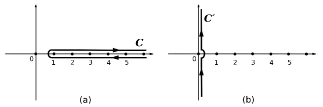
Figure 1: The contours of integration in the complex plane used for summing the series: (a) the original contour ${\cal C}$; (b) the deformed contour ${\cal C}^{\prime}$;

To perform the summations over $m_{\alpha}$ and $s_{\alpha}$ in eq.(57) it is convenient to represent it in the following way:

$$V_{x}(f_{1},f_{2})\;=\;1+\sum_{M=1}^{\infty}\;\frac{(-1)^{M}}{M!}\;\prod_{\alpha=1}^{M}\Biggl{[}\int\int_{-\infty}^{+\infty}\frac{dy_{\alpha}dp_{\alpha}}{2\pi}\operatorname{Ai}\bigl{(}y_{\alpha}+p_{\alpha}^{2}-ixp_{\alpha}\bigr{)}\Biggr{]}\;{\cal S}_{M}\bigl{(}{\bf p},{\bf y};\;f_{1},f_{2}\bigr{)}$$ (62)

where

$${\cal S}_{M}\bigl{(}{\bf p},{\bf y};\;f_{1},f_{2}\bigr{)} = \lim_{\lambda\to\infty}\prod_{\alpha=1}^{M}\Biggl{[}\sum_{m_{\alpha}+s_{\alpha}\geq 1}^{\infty}(-1)^{m_{\alpha}+s_{\alpha}-1}\exp\Bigl{\{}\lambda m_{\alpha}\bigl{(}y_{\alpha}+f_{1}\bigr{)}+\lambda s_{\alpha}\bigl{(}y_{\alpha}+f_{2}\bigr{)}\Bigr{\}}\Biggr{]}\times$$ (63)

$$\times \prod_{\alpha=1}^{M}\Biggl{[}{\cal G}\Bigl{(}\frac{p_{\alpha}}{\lambda},\;m_{\alpha},\;s_{\alpha}\Bigr{)}\;\Biggr{]}\;\det\hat{K}\bigl{[}(\lambda m_{\alpha},\lambda s_{\alpha},p_{\alpha});(\lambda m_{\beta},\lambda s_{\beta},p_{\beta})\bigr{]}\;{\bf G}_{M}\Bigl{(}\frac{{\bf p}}{\lambda},\;{\bf m},\;{\bf s}\Bigr{)}$$

The summations over $m_{\alpha}$ and $s_{\alpha}$ in the above expression can be represented as follows

$$\sum_{m_{\alpha}+s_{\alpha}\geq 1}^{\infty}(-1)^{m_{\alpha}+s_{\alpha}-1}=\sum_{m_{\alpha}=1}^{\infty}(-1)^{m_{\alpha}-1}\delta(s_{\alpha},0)+\sum_{s_{\alpha}=1}^{\infty}(-1)^{s_{\alpha}-1}\delta(m_{\alpha},0)-\sum_{m_{\alpha}=1}^{\infty}(-1)^{m_{\alpha}-1}\sum_{s_{\alpha}=1}^{\infty}(-1)^{s_{\alpha}-1}$$ (64)

Thus in the integral representation, eqs.(59)-(61), for the function ${\cal S}_{M}\bigl{(}{\bf p},{\bf y};\;f_{1},f_{2}\bigr{)}$, eq.(63), we get

$${\cal S}_{M}\bigl{(}{\bf p},{\bf y};\;f_{1},f_{2}\bigr{)} = \prod_{\alpha=1}^{M}\Biggl{[}\int\int_{{\cal C}^{\prime}}\frac{d{z_{1}}_{\alpha}d{z_{2}}_{\alpha}}{(2\pi i)^{2}}\Bigl{(}\frac{2\pi i}{{z_{1}}_{\alpha}}\delta({z_{2}}_{\alpha})+\frac{2\pi i}{{z_{2}}_{\alpha}}\delta({z_{1}}_{\alpha})-\frac{1}{{z_{1}}_{\alpha}{z_{2}}_{\alpha}}\Bigr{)}\exp\Bigl{\{}{z_{1}}_{\alpha}\bigl{(}y_{\alpha}+f_{1}\bigr{)}+{z_{2}}_{\alpha}\bigl{(}y_{\alpha}+f_{2}\bigr{)}\Bigr{\}}\Biggr{]}\times$$ (65)

$$= \lim_{\lambda\to\infty}\Biggl{\{}\prod_{\alpha=1}^{M}\Biggl{[}{\cal G}\Bigl{(}\frac{p_{\alpha}}{\lambda},\;\frac{{z_{1}}_{\alpha}}{\lambda},\;\frac{{z_{2}}_{\alpha}}{\lambda}\Bigr{)}\;\Biggr{]}\;{\bf G}_{M}\Bigl{(}\frac{{\bf p}}{\lambda},\;\frac{{\bf z_{1}}}{\lambda},\;\frac{{\bf z_{2}}}{\lambda}\Bigr{)}\Biggr{\}}\;\det\hat{K}\bigl{[}({z_{1}}_{\alpha},{z_{2}}_{\alpha},p_{\alpha});({z_{1}}_{\beta},{z_{2}}_{\beta},p_{\beta})\bigr{]}\;$$

Taking into account the Gamma function properties, $\Gamma(z)|_{|z|\to 0}=1/z$ and $\Gamma(1+z)|_{|z|\to 0}=1$, for the factors ${\cal G}$, eq.(49), and ${\bf G}$, eq.(A.17), we obtain

$$\lim_{\lambda\to\infty}{\cal G}\Bigl{(}\frac{p_{\alpha}}{\lambda},\;\frac{{z_{1}}_{\alpha}}{\lambda},\;\frac{{z_{2}}_{\alpha}}{\lambda}\Bigr{)}\;=\;\frac{\bigl{(}{z_{1}}_{\alpha}+{z_{2}}_{\alpha}+ip_{\alpha}^{(-)}\bigr{)}\bigl{(}{z_{1}}_{\alpha}+{z_{2}}_{\alpha}-ip_{\alpha}^{(+)}\bigr{)}}{\bigl{(}{z_{2}}_{\alpha}+ip_{\alpha}^{(-)}\bigr{)}\bigl{(}{z_{1}}_{\alpha}-ip_{\alpha}^{(+)}\bigr{)}}$$ (66)

and

$$\lim_{\lambda\to\infty}{\bf G}\Bigl{(}\frac{{\bf p}}{\lambda},\;\frac{{\bf z}_{1}}{\lambda},\;\frac{{\bf z}_{2}}{\lambda}\Bigr{)}\;=\;1$$ (67)

Thus, in the limit $\lambda\to\infty$ the expression for the probability distribution function, eq.(62), takes the form of the Fredholm determinant

$$V_{x}(f_{1},f_{2}) = 1+\sum_{M=1}^{\infty}\;\frac{(-1)^{M}}{M!}\;\prod_{\alpha=1}^{M}\Biggl{[}\int\int_{-\infty}^{+\infty}\frac{dy_{\alpha}dp_{\alpha}}{2\pi}\operatorname{Ai}\bigl{(}y_{\alpha}+p_{\alpha}^{2}-ixp_{\alpha}\bigr{)}\times$$ (68)

$$\times \int\int_{{\cal C}^{\prime}}\frac{d{z_{1}}_{\alpha}d{z_{2}}_{\alpha}}{(2\pi i)^{2}}\Bigl{(}\frac{2\pi i}{{z_{1}}_{\alpha}}\delta({z_{2}}_{\alpha})+\frac{2\pi i}{{z_{2}}_{\alpha}}\delta({z_{1}}_{\alpha})-\frac{1}{{z_{1}}_{\alpha}{z_{2}}_{\alpha}}\Bigr{)}\Bigl{(}1+\frac{{z_{1}}_{\alpha}}{{z_{2}}_{\alpha}+ip_{\alpha}^{(-)}}\Bigr{)}\Bigl{(}1+\frac{{z_{2}}_{\alpha}}{{z_{1}}_{\alpha}-ip_{\alpha}^{(+)}}\Bigr{)}\times$$

$$\times \exp\Bigl{\{}{z_{1}}_{\alpha}\bigl{(}y_{\alpha}+f_{1}\bigr{)}+{z_{2}}_{\alpha}\bigl{(}y_{\alpha}+f_{2}\bigr{)}\Bigr{\}}\Biggr{]}\det\Bigl{[}\frac{1}{{z_{1}}_{\alpha}+{z_{2}}_{\alpha}-ip_{\alpha}+{z_{1}}_{\beta}+{z_{2}}_{\beta}+ip_{\beta}}\Bigr{]}_{(\alpha,\beta)=1,2,...,M}$$

$$= \det\bigl{[}\hat{1}\,-\,\hat{A}\bigr{]}$$

with the kernel

$$\hat{A}\bigl{[}({z_{1}},\,{z_{2}},\,p);({z_{1}}^{\prime},\,{z_{2}}^{\prime},\,p^{\prime})\bigr{]} = \int_{-\infty}^{+\infty}\frac{dy}{2\pi}\operatorname{Ai}\bigl{(}y+p^{2}-ixp\bigr{)}\Bigl{(}\frac{2\pi i}{z_{1}}\delta(z_{2})+\frac{2\pi i}{z_{2}}\delta(z_{1})-\frac{1}{z_{1}{z_{2}}}\Bigr{)}\times$$ (69)

$$\times \Bigl{(}1+\frac{z_{1}}{z_{2}+ip^{(-)}}\Bigr{)}\Bigl{(}1+\frac{z_{2}}{z_{1}-ip^{(+)}}\Bigr{)}\exp\Bigl{\{}z_{1}\bigl{(}y+f_{1}\bigr{)}+z_{2}\bigl{(}y+f_{2}\bigr{)}\Bigr{\}}\times$$

$$\times \frac{1}{{z_{1}}+{z_{2}}-ip+{z_{1}}^{\prime}+{z_{2}}^{\prime}+ip^{\prime}}$$

In the exponential representation of this determinant we get

$$V_{x}(f_{1},f_{2})\;=\;\exp\Bigl{[}-\sum_{M=1}^{\infty}\frac{1}{M}\;\mbox{Tr}\,\hat{A}^{M}\Bigr{]}$$ (70)

where

$$\mbox{Tr}\,\hat{A}^{M} = \prod_{\alpha=1}^{M}\Biggl{[}\int\int_{-\infty}^{+\infty}\frac{dy_{\alpha}dp_{\alpha}}{2\pi}\operatorname{Ai}\bigl{(}y_{\alpha}+p_{\alpha}^{2}-ixp_{\alpha}\bigr{)}\times$$ (71)

$$\times \int\int_{{\cal C}^{\prime}}\frac{d{z_{1}}_{\alpha}d{z_{2}}_{\alpha}}{(2\pi i)^{2}}\Bigl{(}\frac{2\pi i}{{z_{1}}_{\alpha}}\delta({z_{2}}_{\alpha})+\frac{2\pi i}{{z_{2}}_{\alpha}}\delta({z_{1}}_{\alpha})-\frac{1}{{z_{1}}_{\alpha}{z_{2}}_{\alpha}}\Bigr{)}\Bigl{(}1+\frac{{z_{1}}_{\alpha}}{{z_{2}}_{\alpha}+ip_{\alpha}^{(-)}}\Bigr{)}\Bigl{(}1+\frac{{z_{2}}_{\alpha}}{{z_{1}}_{\alpha}-ip_{\alpha}^{(+)}}\Bigr{)}\times$$

$$\times \exp\Bigl{\{}{z_{1}}_{\alpha}\bigl{(}y_{\alpha}+f_{1}\bigr{)}+{z_{2}}_{\alpha}\bigl{(}y_{\alpha}+f_{2}\bigr{)}\Bigr{\}}\Biggr{]}\;\prod_{\alpha=1}^{M}\Biggl{[}\frac{1}{{z_{1}}_{\alpha}+{z_{2}}_{\alpha}-ip_{\alpha}+{z_{1}}_{\alpha+1}+{z_{2}}_{\alpha+1}+ip_{\alpha+1}}\Biggr{]}$$

Here, by definition, it is assumed that ${z_{i_{M+1}}}\equiv{z_{i_{1}}}$ ($i=1,2$) and $p_{M+1}\equiv p_{1}$. Substituting

$$\frac{1}{{z_{1}}_{\alpha}+{z_{2}}_{\alpha}-ip_{\alpha}+{z_{1}}_{\alpha+1}+{z_{2}}_{\alpha+1}+ip_{\alpha+1}}\;=\;\int_{0}^{\infty}d\omega_{\alpha}\exp\Bigl{[}-\bigl{(}{z_{1}}_{\alpha}+{z_{2}}_{\alpha}-ip_{\alpha}+{z_{1}}_{\alpha+1}+{z_{2}}_{\alpha+1}+ip_{\alpha+1}\bigr{)}\,\omega_{\alpha}\Bigr{]}$$ (72)

into eq.(71), we obtain

$$\mbox{Tr}\,\hat{A}^{M}\;=\;\int_{0}^{\infty}d\omega_{1}\,...\,d\omega_{M}\,\prod_{\alpha=1}^{M}\Biggl{[}\int\int_{-\infty}^{+\infty}\frac{dydp}{2\pi}\operatorname{Ai}\bigl{(}y+p^{2}+\omega_{\alpha}+\omega_{\alpha-1}-ixp\bigr{)}\exp\{ip\bigl{(}\omega_{\alpha}-\omega_{\alpha-1}\bigr{)}\}\;S\bigl{(}p,y;f_{1},f_{2}\bigr{)}\Biggr{]}$$ (73)

where, by definition, $\omega_{0}\equiv\omega_{M}$, and

$$S(p,y;f_{1},f_{2}) = \int\int_{{\cal C}^{\prime}}\frac{dz_{1}dz_{2}}{(2\pi i)^{2}}\Bigl{(}\frac{2\pi i}{z_{1}}\delta(z_{2})+\frac{2\pi i}{z_{2}}\delta(z_{1})-\frac{1}{z_{1}z_{2}}\Bigr{)}\Bigl{(}1+\frac{z_{1}}{z_{2}+ip^{(-)}}\Bigr{)}\Bigl{(}1+\frac{z_{2}}{z_{1}-ip^{(+)}}\Bigr{)}\times$$ (74)

$$\times \exp\Bigl{\{}z_{1}\bigl{(}y+f_{1}\bigr{)}+z_{2}\bigl{(}y+f_{2}\bigr{)}\Bigr{\}}$$

Simple integrations provide the following result:

$$S(p,y;f_{1},f_{2}) = \theta(y+f_{1})+\theta(y+f_{2})-\theta(y+f_{1})\theta(y+f_{2})-\theta(y+f_{1})\theta(y+f_{2})\exp\bigl{\{}ip(f_{1}-f_{2})-2\epsilon y\bigr{\}}$$ (75)

$$+ \frac{i}{p+i\epsilon}\delta(y+f_{2})-\frac{i}{p-i\epsilon}\delta(y+f_{1})$$

$$- \frac{i}{p+i\epsilon}\delta(y+f_{2})\theta(f_{1}-f_{2})\Bigl{[}1-\exp\{i(p+i\epsilon)(f_{1}-f_{2})\}\Bigr{]}$$

$$+ \frac{i}{p-i\epsilon}\delta(y+f_{1})\theta(f_{2}-f_{1})\bigl{[}1-\exp\{i(p-i\epsilon)(f_{1}-f_{2})\}\bigr{]}$$

According to eq.(17) in what follows we will be dealing with the sector $f_{2}>f_{1}$ only. In this case the above expression simplifies to

$$S(p,y;f_{1},f_{2})\big{|}_{f_{2}>f_{1}} = \Bigl{(}\frac{i}{p+i\epsilon}-\frac{i}{p-i\epsilon}\Bigr{)}\delta(y+f_{2})$$ (76)

$$+ \frac{i}{p-i\epsilon}\Bigl{[}\delta(y+f_{2})-\delta(y+f_{1})\exp\{ip(f_{1}-f_{2})\}\Bigr{]}$$

$$+ \theta(y+f_{2})-\theta(y+f_{1})\exp\{ip(f_{1}-f_{2})-2\epsilon y\}$$

Note that at edge of the sector $f_{2}>f_{1}$ for $f_{2}=f_{1}+0$ (in the limit $\epsilon\to 0$)

$$S(p,y;f_{1},f_{2})\big{|}_{f_{2}=f_{1}+0}\;=\;2\pi\delta(p)\delta(y+f_{2})$$ (77)

Thus, according to eqs.(73) and (76), the two-point free energy distribution function $V_{x}(f_{1},f_{2})$, eq.(14), (in the sector $f_{2}>f_{1}$) is given by the Fredholm determinant, eq.(70), with the kernel

$$A(\omega,\omega^{\prime}) = \operatorname{Ai}(\omega+\omega^{\prime}-f_{2})-$$ (78)

$$- \int_{-\infty}^{+\infty}\frac{dp}{2\pi}\frac{\Bigl{[}\operatorname{Ai}(\omega+\omega^{\prime}+p^{2}-ipx-f_{2})-\operatorname{Ai}(\omega+\omega^{\prime}+p^{2}-ipx-f_{1})\exp\{ip(f_{1}-f_{2})\}\Bigr{]}}{i(p-i\epsilon)}\exp\{ip\bigl{(}\omega-\omega^{\prime}\bigr{)}\}+$$

$$+ \int_{-\infty}^{+\infty}\frac{dp}{2\pi}\Biggl{[}\int_{-f_{2}}^{+\infty}dy\operatorname{Ai}(\omega+\omega^{\prime}+p^{2}-ipx+y)-\int_{-f_{1}}^{+\infty}dy\operatorname{Ai}(\omega+\omega^{\prime}+p^{2}-ipx+y)\exp\{ip(f_{1}-f_{2})\}\Biggr{]}\times$$

$$\times \exp\{ip\bigl{(}\omega-\omega^{\prime}\bigr{)}\}$$

with $\omega,\omega^{\prime}>0$.

V The endpoint probability distribution function

Substituting the above result, eqs.(70) and (78), into eq.(17) for the endpoint distribution function one obtains the following expression:

$$W(x)\;=\;\int_{-\infty}^{+\infty}df\;F_{1}(-f)\int_{0}^{+\infty}d\omega\int_{0}^{+\infty}d\omega^{\prime}\Bigl{(}\hat{1}-\hat{B}_{-f}\Bigr{)}^{-1}(\omega,\omega^{\prime})\;\Phi(\omega^{\prime},\omega;f,x)$$ (79)

where

$$F_{1}(-f)=\det\bigl{[}\hat{1}\,-\,\hat{B}_{-f}\bigr{]}\;=\;\exp\Bigl{[}-\sum_{M=1}^{\infty}\frac{1}{M}\;\mbox{Tr}\,\hat{B}_{-f}^{M}\Bigr{]}$$ (80)

is the GOE Tracy-Widom distribution with the kernel

$$B_{-f}(\omega,\omega^{\prime})\;=\;\operatorname{Ai}(\omega+\omega^{\prime}-f),\;\;\;\;\;\;\;(\omega,\omega^{\prime}\,>\,0)$$ (81)

and

$$\Phi(\omega,\omega^{\prime};f,x) = i\int_{-\infty}^{+\infty}\frac{dp}{2\pi}\;\frac{1}{p-i\epsilon}\;\operatorname{Ai}^{\prime}(\omega+\omega^{\prime}+p^{2}-ipx-f)\;\exp\{ip\bigl{(}\omega-\omega^{\prime}\bigr{)}\}$$ (82)

$$- i\int_{-f}^{+\infty}dy\;\int_{-\infty}^{+\infty}\frac{dp}{2\pi}\,p\,\operatorname{Ai}(\omega+\omega^{\prime}+p^{2}-ipx+y)\;\exp\{ip\bigl{(}\omega-\omega^{\prime}\bigr{)}\}$$

Using the standard integral representation of the Airy function one can easily reduce the above function $\Phi(\omega,\omega^{\prime};f,x)$ to the following sufficiently simple form:

$$\Phi(\omega,\omega^{\prime};f,x)=-\frac{1}{2}\int_{0}^{+\infty}dy\; \Biggl{[} \Bigl{(}\frac{\partial}{\partial\omega}-\frac{\partial}{\partial\omega^{\prime}}\Bigr{)}\Psi\bigl{(}\omega-\frac{1}{2}f+y;\;x\bigr{)}\Psi\bigl{(}\omega^{\prime}-\frac{1}{2}f+y;\;-x\bigr{)}+$$ (83)

$$+ \Bigl{(}\frac{\partial}{\partial\omega}+\frac{\partial}{\partial\omega^{\prime}}\Bigr{)}\Psi\bigl{(}\omega-\frac{1}{2}f-y;\;x\bigr{)}\Psi\bigl{(}\omega^{\prime}-\frac{1}{2}f+y;\;-x\bigr{)}\Biggr{]}$$

where

$$\Psi(\omega;x)\;=\;2^{1/3}\mbox{Ai}\Bigl{[}2^{1/3}\bigl{(}\omega+\frac{1}{8}x^{2}\bigr{)}\Bigr{]}\,\exp\bigl{\{}-\frac{1}{2}\omega x\bigr{\}}$$ (84)

Thus, eqs.(79), (83) and (84) complete the derivation of the probability distribution function for the directed polymer’s endpoint. Unfortunately, at present stage the analytical properties of this function are not quite clear. The study of this function require the special analysis and it will be done elsewhere.

VI Conclusions

In this paper the explicit expression for the the probability distribution function of the endpoint of one-dimensional directed polymers in random potential is derived in terms of the Bethe ansatz replica technique. The result obtained, eqs.(79)-(84), looks quite similar to the one derived in terms of completely different method in which the maximal point of the $\mbox{Airy}_{2}$ process minus a parabola is considered math1 ; math2 ; math3 . Unfortunately, at present stage the final expression for the probability distribution function obtained both here and in Refs.math1 ; math2 ; math3 is rather sophisticated so that the study of its analytical properties would require special efforts. Hopefully this problem will be solved in the near future.

One more conclusion of the present study is that the approach used, namely the Bethe ansatz replica technique, once again (following the works BA-replicas ; LeDoussal1 ; LeDoussal2 ; goe ) has demonstrated its efficiency. Hopefully it will also be fruitful for the studies of more serious problems in this scope, such as joint statistical properties of the free energy fluctuations at different times.

$$\prod_{a=1}^{L}q^{(-)}_{{\cal P}_{a}^{(L)}} = \prod_{\alpha=1}^{M}\prod_{r=1}^{m_{\alpha}}{q^{\alpha}_{r}}^{(-)}$$ (A.1)

$$\prod_{a=1}^{R}q^{(+)}_{{\cal P}_{a}^{(R)}} = \prod_{\alpha=1}^{M}\prod_{r=1}^{s_{\alpha}}{{q^{*}}^{\alpha}_{r}}^{(+)}$$ (A.2)

$$\prod_{a<b}^{L}\Biggl{[}\frac{q^{(-)}_{{\cal P}_{a}^{(L)}}+q^{(-)}_{{\cal P}_{b}^{(L)}}+i\kappa}{q^{(-)}_{{\cal P}_{a}^{(L)}}+q^{(-)}_{{\cal P}_{b}^{(L)}}}\Biggr{]} = \prod_{\alpha=1}^{M}\prod_{1\leq r<r^{\prime}}^{m_{\alpha}}\Biggl{[}\frac{{q^{\alpha}_{r}}^{(-)}+{q^{\alpha}_{r^{\prime}}}^{(-)}+i\kappa}{{q^{\alpha}_{r}}^{(-)}+{q^{\alpha}_{r^{\prime}}}^{(-)}}\Biggr{]}\times\prod_{1\leq\alpha<\beta}^{M}\prod_{r=1}^{m_{\alpha}}\prod_{r^{\prime}=1}^{m_{\beta}}\Biggl{[}\frac{{q^{\alpha}_{r}}^{(-)}+{q^{\beta}_{r^{\prime}}}^{(-)}+i\kappa}{{q^{\alpha}_{r}}^{(-)}+{q^{\beta}_{r^{\prime}}}^{(-)}}\Biggr{]}$$ (A.3)

$$\prod_{c<d}^{R}\Biggl{[}\frac{q^{(+)}_{{\cal P}_{c}^{(R)}}+q^{(+)}_{{\cal P}_{d}^{(R)}}-i\kappa}{q^{(+)}_{{\cal P}_{c}^{(R)}}+q^{(+)}_{{\cal P}_{d}^{(R)}}}\Biggr{]} = \prod_{\alpha=1}^{M}\prod_{1\leq r<r^{\prime}}^{s_{\alpha}}\Biggl{[}\frac{{{q^{*}}^{\alpha}_{r}}^{(+)}+{{q^{*}}^{\alpha}_{r^{\prime}}}^{(+)}-i\kappa}{{{q^{*}}^{\alpha}_{r}}^{(+)}+{{q^{*}}^{\alpha}_{r^{\prime}}}^{(+)}}\Biggr{]}\times\prod_{1\leq\alpha<\beta}^{M}\prod_{r=1}^{s_{\alpha}}\prod_{r^{\prime}=1}^{s_{\beta}}\Biggl{[}\frac{{{q^{*}}^{\alpha}_{r}}^{(+)}+{{q^{*}}^{\beta}_{r^{\prime}}}^{(+)}-i\kappa}{{{q^{*}}^{\alpha}_{r}}^{(+)}+{{q^{*}}^{\beta}_{r^{\prime}}}^{(+)}}\Biggr{]}$$ (A.4)

$$\prod_{a=1}^{L}\prod_{c=1}^{R}\Biggl{[}\frac{q_{{\cal P}_{a}^{(L)}}-q_{{\cal P}_{c}^{(R)}}-i\kappa}{q_{{\cal P}_{a}^{(L)}}-q_{{\cal P}_{c}^{(R)}}}\Biggr{]} = \prod_{1\leq\alpha<\beta}^{M}\Biggl{\{}\prod_{r=1}^{m_{\alpha}}\prod_{r^{\prime}=1}^{s_{\beta}}\Biggl{[}\frac{q^{\alpha}_{r}-{q^{*}}^{\beta}_{r^{\prime}}-i\kappa}{q^{\alpha}_{r}+{q^{*}}^{\beta}_{r^{\prime}}}\Biggr{]}\times\prod_{r=1}^{s_{\alpha}}\prod_{r^{\prime}=1}^{m_{\beta}}\Biggl{[}\frac{{q^{*}}^{\alpha}_{r}-q^{\beta}_{r^{\prime}}-i\kappa}{{q^{*}}^{\alpha}_{r}-q^{\beta}_{r^{\prime}}}\Biggr{]}\Biggr{\}}\times$$ (A.5)

$$\times \prod_{\alpha=1}^{M}\prod_{r=1}^{m_{\alpha}}\prod_{r^{\prime}=1}^{s_{\alpha}}\Biggl{[}\frac{q^{\alpha}_{r}-{q^{*}}^{\alpha}_{r^{\prime}}-i\kappa}{q^{\alpha}_{r}-{q^{*}}^{\alpha}_{r^{\prime}}}\Biggr{]}$$

Substituting eqs.(A.1)-(A.5) into eq.(41), and then substituting the resulting expression into eq.(IV) we obtain eq.(47) where

$${\cal G}\bigl{(}q_{\alpha},m_{\alpha},s_{\alpha}\bigr{)} = \frac{(-1)^{s_{\alpha}}(-i\kappa)^{(m_{\alpha}+s_{\alpha})}}{\prod_{r=1}^{m_{\alpha}}{q^{\alpha}_{r}}^{(-)}\prod_{r=1}^{s_{\alpha}}{{q^{*}}^{\alpha}_{r}}^{(+)}}\times$$ (A.6)

$$\times \prod_{r<r^{\prime}}^{m_{\alpha}}\Biggl{[}\frac{{q^{\alpha}_{r}}^{(-)}+{q^{\alpha}_{r^{\prime}}}^{(-)}+i\kappa}{{q^{\alpha}_{r}}^{(-)}+{q^{\alpha}_{r^{\prime}}}^{(-)}}\Biggr{]}\prod_{r<r^{\prime}}^{s_{\alpha}}\Biggl{[}\frac{{{q^{*}}^{\alpha}_{r}}^{(+)}+{{q^{*}}^{\alpha}_{r^{\prime}}}^{(+)}-i\kappa}{{{q^{*}}^{\alpha}_{r}}^{(+)}+{{q^{*}}^{\alpha}_{r^{\prime}}}^{(+)}}\Biggr{]}\prod_{r=1}^{m_{\alpha}}\prod_{r^{\prime}=1}^{s_{\alpha}}\Biggl{[}\frac{q^{\alpha}_{r}-{q^{*}}^{\alpha}_{r^{\prime}}-i\kappa}{q^{\alpha}_{r}-{q^{*}}^{\alpha}_{r^{\prime}}}\Biggr{]}$$

and

$${\bf G}_{M}\bigl{(}{\bf q},{\bf m},{\bf s}\bigr{)} = \prod_{1\leq\alpha<\beta}^{M}\Biggl{\{}\prod_{r=1}^{m_{\alpha}}\prod_{r^{\prime}=1}^{m_{\beta}}\Biggl{[}\frac{{q^{\alpha}_{r}}^{(-)}+{q^{\beta}_{r^{\prime}}}^{(-)}+i\kappa}{{q^{\alpha}_{r}}^{(-)}+{q^{\beta}_{r^{\prime}}}^{(-)}}\Biggr{]}\prod_{r=1}^{s_{\alpha}}\prod_{r^{\prime}=1}^{s_{\beta}}\Biggl{[}\frac{{{q^{*}}^{\alpha}_{r}}^{(+)}+{{q^{*}}^{\beta}_{r^{\prime}}}^{(+)}-i\kappa}{{{q^{*}}^{\alpha}_{r}}^{(+)}+{{q^{*}}^{\beta}_{r^{\prime}}}^{(+)}}\Biggr{]}\times$$ (A.7)

$$\times \prod_{r=1}^{m_{\alpha}}\prod_{r^{\prime}=1}^{s_{\beta}}\Biggl{[}\frac{q^{\alpha}_{r}-{q^{*}}^{\beta}_{r^{\prime}}-i\kappa}{q^{\alpha}_{r}+{q^{*}}^{\beta}_{r^{\prime}}}\Biggr{]}\times\prod_{r=1}^{s_{\alpha}}\prod_{r^{\prime}=1}^{m_{\beta}}\Biggl{[}\frac{{q^{*}}^{\alpha}_{r}-q^{\beta}_{r^{\prime}}-i\kappa}{{q^{*}}^{\alpha}_{r}-q^{\beta}_{r^{\prime}}}\Biggr{]}\Biggr{\}}$$

The product factors in eq.(A.6) can be easily expressed it terms of the Gamma functions:

$$\prod_{r=1}^{m_{\alpha}}{q^{\alpha}_{r}}^{(-)} = \prod_{r=1}^{m_{\alpha}}\Bigl{[}{q_{\alpha}}^{(-)}-\frac{i\kappa}{2}(m_{\alpha}+s_{\alpha}+1)+i\kappa r\Bigr{]}\;=\;(i\kappa)^{m_{\alpha}}\frac{\Gamma\Bigl{(}\frac{1}{2}-\frac{s_{\alpha}-m_{\alpha}}{2}-\frac{i{q_{\alpha}}^{(-)}}{\kappa}\Bigr{)}}{\Gamma\Bigl{(}\frac{1}{2}-\frac{s_{\alpha}+m_{\alpha}}{2}-\frac{i{q_{\alpha}}^{(-)}}{\kappa}\Bigr{)}}$$ (A.8)

$$\prod_{r=1}^{s_{\alpha}}{{q^{*}}^{\alpha}_{r}}^{(+)} = \prod_{r=1}^{s_{\alpha}}\Bigl{[}{q_{\alpha}}^{(+)}+\frac{i\kappa}{2}(m_{\alpha}+s_{\alpha}+1)-i\kappa r\Bigr{]}\;=\;(-i\kappa)^{s_{\alpha}}\frac{\Gamma\Bigl{(}\frac{1}{2}-\frac{m_{\alpha}-s_{\alpha}}{2}+\frac{i{q_{\alpha}}^{(+)}}{\kappa}\Bigr{)}}{\Gamma\Bigl{(}\frac{1}{2}-\frac{m_{\alpha}+s_{\alpha}}{2}+\frac{i{q_{\alpha}}^{(+)}}{\kappa}\Bigr{)}}$$ (A.9)

$$\prod_{r<r^{\prime}}^{m_{\alpha}}\Biggl{[}\frac{{q^{\alpha}_{r}}^{(-)}+{q^{\alpha}_{r^{\prime}}}^{(-)}+i\kappa}{{q^{\alpha}_{r}}^{(-)}+{q^{\alpha}_{r^{\prime}}}^{(-)}}\Biggr{]} = 2^{-(m_{\alpha}-1)}\frac{\Gamma\Bigl{(}m_{\alpha}-s_{\alpha}-\frac{2i{q_{\alpha}}^{(-)}}{\kappa}\Bigr{)}\Gamma\Bigl{(}1-\frac{m_{\alpha}+s_{\alpha}}{2}-\frac{i{q_{\alpha}}^{(-)}}{\kappa}\Bigr{)}}{\Gamma\Bigl{(}\frac{m_{\alpha}-s_{\alpha}}{2}-\frac{i{q_{\alpha}}^{(-)}}{\kappa}\Bigr{)}\Gamma\Bigl{(}1-s_{\alpha}-\frac{2i{q_{\alpha}}^{(-)}}{\kappa}\Bigr{)}}$$ (A.10)

$$\prod_{r<r^{\prime}}^{s_{\alpha}}\Biggl{[}\frac{{{q^{*}}^{\alpha}_{r}}^{(+)}+{{q^{*}}^{\alpha}_{r^{\prime}}}^{(+)}-i\kappa}{{{q^{*}}^{\alpha}_{r}}^{(+)}+{{q^{*}}^{\alpha}_{r^{\prime}}}^{(+)}}\Biggr{]} = 2^{-(s_{\alpha}-1)}\frac{\Gamma\Bigl{(}s_{\alpha}-m_{\alpha}+\frac{2i{q_{\alpha}}^{(+)}}{\kappa}\Bigr{)}\Gamma\Bigl{(}1-\frac{m_{\alpha}+s_{\alpha}}{2}+\frac{i{q_{\alpha}}^{(+)}}{\kappa}\Bigr{)}}{\Gamma\Bigl{(}\frac{s_{\alpha}-m_{\alpha}}{2}+\frac{i{q_{\alpha}}^{(+)}}{\kappa}\Bigr{)}\Gamma\Bigl{(}1-m_{\alpha}+\frac{2i{q_{\alpha}}^{(+)}}{\kappa}\Bigr{)}}$$ (A.11)

$$\prod_{r=1}^{m_{\alpha}}\prod_{r^{\prime}=1}^{s_{\alpha}}\Biggl{[}\frac{q^{\alpha}_{r}-{q^{*}}^{\alpha}_{r^{\prime}}-i\kappa}{q^{\alpha}_{r}-{q^{*}}^{\alpha}_{r^{\prime}}}\Biggr{]} = \frac{\Gamma\bigl{(}1+m_{\alpha}+s_{\alpha}\bigr{)}}{\Gamma\bigl{(}1+m_{\alpha}\bigr{)}\Gamma\bigl{(}1+s_{\alpha}\bigr{)}}$$ (A.12)

Substituting the above expressions into eq.(A.6) and using the standard relations for the Gamma functions,

$$\Gamma(z)\,\Gamma(1-z) = \frac{\pi}{\sin(\pi z)}$$ (A.13)

$$\Gamma(1+z) = z\,\Gamma(z)$$ (A.14)

$$\Gamma\Bigl{(}\frac{1}{2}+z\Bigr{)} = \frac{\sqrt{\pi}\,\Gamma\bigl{(}1+2z\bigr{)}}{2^{2z}\,\Gamma\bigl{(}1+z\bigr{)}}$$ (A.15)

for the factor ${\cal G}$, eq.(A.6), we get

$${\cal G}\bigl{(}q_{\alpha},m_{\alpha},s_{\alpha}\bigr{)}\;=\;\frac{\Gamma\Bigl{(}s_{\alpha}+\frac{2i}{\kappa}{q_{\alpha}}^{(-)}\Bigr{)}\,\Gamma\Bigl{(}m_{\alpha}-\frac{2i}{\kappa}{q_{\alpha}}^{(+)}\Bigr{)}\,\Gamma\bigl{(}1+m_{\alpha}+s_{\alpha}\bigr{)}}{2^{(m_{\alpha}+s_{\alpha})}\Gamma\Bigl{(}m_{\alpha}+s_{\alpha}+\frac{2i}{\kappa}{q_{\alpha}}^{(-)}\Bigr{)}\,\Gamma\Bigl{(}m_{\alpha}+s_{\alpha}-\frac{2i}{\kappa}{q_{\alpha}}^{(+)}\Bigr{)}\,\Gamma\bigl{(}1+m_{\alpha}\bigr{)}\Gamma\bigl{(}1+s_{\alpha}\bigr{)}}$$ (A.16)

Similar calculations for the factor ${\bf G}_{M}$, eq.(A.7) yield the following expression

$${\bf G}_{M}\bigl{(}{\bf q},{\bf m},{\bf s}\bigr{)} = \prod_{1\leq\alpha<\beta}^{M}\Biggl{\{}\frac{\Gamma\Bigl{[}1+\frac{m_{\alpha}+m_{\beta}-s_{\alpha}-s_{\beta}}{2}-\frac{i}{\kappa}\bigl{(}{q_{\alpha}}^{(-)}+{q_{\beta}}^{(-)}\bigr{)}\Bigr{]}\,\Gamma\Bigl{[}1-\frac{m_{\alpha}+m_{\beta}+s_{\alpha}+s_{\beta}}{2}-\frac{i}{\kappa}\bigl{(}{q_{\alpha}}^{(-)}+{q_{\beta}}^{(-)}\bigr{)}\Bigr{]}}{\Gamma\Bigl{[}1-\frac{m_{\alpha}-m_{\beta}+s_{\alpha}+s_{\beta}}{2}-\frac{i}{\kappa}\bigl{(}{q_{\alpha}}^{(-)}+{q_{\beta}}^{(-)}\bigr{)}\Bigr{]}\,\Gamma\Bigl{[}1+\frac{m_{\alpha}-m_{\beta}-s_{\alpha}-s_{\beta}}{2}-\frac{i}{\kappa}\bigl{(}{q_{\alpha}}^{(-)}+{q_{\beta}}^{(-)}\bigr{)}\Bigr{]}}\times$$ (A.17)

$$\times \frac{\Gamma\Bigl{[}1-\frac{m_{\alpha}+m_{\beta}-s_{\alpha}-s_{\beta}}{2}+\frac{i}{\kappa}\bigl{(}{q_{\alpha}}^{(+)}+{q_{\beta}}^{(+)}\bigr{)}\Bigr{]}\,\Gamma\Bigl{[}1-\frac{m_{\alpha}+m_{\beta}+s_{\alpha}+s_{\beta}}{2}+\frac{i}{\kappa}\bigl{(}{q_{\alpha}}^{(+)}+{q_{\beta}}^{(+)}\bigr{)}\Bigr{]}}{\Gamma\Bigl{[}1-\frac{m_{\alpha}+m_{\beta}+s_{\alpha}-s_{\beta}}{2}+\frac{i}{\kappa}\bigl{(}{q_{\alpha}}^{(+)}+{q_{\beta}}^{(+)}\bigr{)}\Bigr{]}\,\Gamma\Bigl{[}1-\frac{m_{\alpha}+m_{\beta}-s_{\alpha}+s_{\beta}}{2}+\frac{i}{\kappa}\bigl{(}{q_{\alpha}}^{(+)}+{q_{\beta}}^{(+)}\bigr{)}\Bigr{]}}\times$$

$$\times \frac{\Gamma\Bigl{[}1+\frac{m_{\alpha}+m_{\beta}+s_{\alpha}+s_{\beta}}{2}+\frac{i}{\kappa}\bigl{(}q_{\alpha}-q_{\beta}\bigr{)}\Bigr{]}\,\Gamma\Bigl{[}1+\frac{-m_{\alpha}+m_{\beta}+s_{\alpha}-s_{\beta}}{2}+\frac{i}{\kappa}\bigl{(}q_{\alpha}-q_{\beta}\bigr{)}\Bigr{]}}{\Gamma\Bigl{[}1+\frac{-m_{\alpha}+m_{\beta}+s_{\alpha}+s_{\beta}}{2}+\frac{i}{\kappa}\bigl{(}q_{\alpha}-q_{\beta}\bigr{)}\Bigr{]}\,\Gamma\Bigl{[}1+\frac{m_{\alpha}+m_{\beta}+s_{\alpha}-s_{\beta}}{2}+\frac{i}{\kappa}\bigl{(}q_{\alpha}-q_{\beta}\bigr{)}\Bigr{]}}\times$$

$$\times \frac{\Gamma\Bigl{[}1+\frac{m_{\alpha}+m_{\beta}+s_{\alpha}+s_{\beta}}{2}-\frac{i}{\kappa}\bigl{(}q_{\alpha}-q_{\beta}\bigr{)}\Bigr{]}\,\Gamma\Bigl{[}1+\frac{m_{\alpha}-m_{\beta}-s_{\alpha}+s_{\beta}}{2}-\frac{i}{\kappa}\bigl{(}q_{\alpha}-q_{\beta}\bigr{)}\Bigr{]}}{\Gamma\Bigl{[}1+\frac{m_{\alpha}+m_{\beta}-s_{\alpha}+s_{\beta}}{2}-\frac{i}{\kappa}\bigl{(}q_{\alpha}-q_{\beta}\bigr{)}\Bigr{]}\,\Gamma\Bigl{[}1+\frac{m_{\alpha}-m_{\beta}+s_{\alpha}+s_{\beta}}{2}-\frac{i}{\kappa}\bigl{(}q_{\alpha}-q_{\beta}\bigr{)}\Bigr{]}}\Biggr{\}}$$

References

• (1) M.Kardar, G.Parisi, Y-C.Zhang, Phys. Rev. Lett. 56, 889 (1986)
• (2) T. Halpin-Healy and Y-C. Zhang, Phys. Rep. 254, 215 (1995).
• (3) J.M. Burgers, The Nonlinear Diffusion Equation (Reidel, Dordrecht, (1974)).
• (4) M. Kardar, ”Statistical physics of fields” (Cambridge: Cambridge University Press, (2007))
• (5) D.A. Huse, C.L. Henley, and D.S. Fisher, Phys. Rev. Lett. 55, 2924 (1985).
• (6) D.A. Huse and C.L. Henley, Phys. Rev. Lett. 54, 2708 (1985).
• (7) M. Kardar and Y-C. Zhang, Phys. Rev. Lett.  58, 2087 (1987).
• (8) M. Kardar, Nucl. Phys. B 290, 582 (1987).
• (9) J. P. Bouchaud and H. Orland, J. Stat. Phys. 61, 877 (1990)
• (10) E. Brunet and B. Derrida, Phys.  Rev.  E 61, 6789 (2000)
• (11) K. Johansson, Comm.  Math.  Phys.  209, 437 (2000)
• (12) M. Prahofer and H. Spohn J. Stat. Phys. 108, 1071 (2002)
• (13) P. L. Ferrari and H. Spohn, Comm.  Math.  Phys.  265, 1 (2006)
• (14) I. Corwin, ”The Kardar-Parisi-Zhang equation and the universality class”, arXiv:1106.1338, Random Matrices: Theory Appl. 1, 1130001 (2012)
• (15) T.Sasamoto and H.Spohn, Phys. Rev. Lett. 104, 230602 (2010); Nucl. Phys. B834, 523 (2010); J. Stat. Phys. 140, 209 (2010)
• (16) G.Amir, I.Corwin and J.Quastel, Comm. Pure Appl. Math. 64, 466 (2011)
• (17) V.Dotsenko and B.Klumov, J.Stat.Mech. P03022 (2010); V.Dotsenko, EPL, 90,20003 (2010); V.Dotsenko, J.Stat.Mech. P07010 (2010)
• (18) P.Calabrese, P. Le Doussal and A.Rosso, EPL, 90,20002 (2010);
• (19) P.Calabrese and P. Le Doussal, Phys. Rev. Lett. 106, 250603 (2011); arXiv:1204.2607
• (20) V.Dotsenko, Replica Bethe ansatz derivation of the GOE Tracy-Widom distribution in one-dimensional directed polymers with free boundary conditions, arXiv:1209.3603; J. Stat. Mech. P11014 (2012)
• (21) G.M.Flores, J.Quastel and D.Remenik, Endpoint distribution of directed polymers in (1+1) domentions, arXiv:1106.2716, Comm. Math. Phys. Online First Articles, November 2012
• (22) G. Schehr, Extremes of N vicious walkers for large N: application to the directed polymer and KPZ interfaces, arXiv:1203.1658, J. Stat. Phys. 149(3), 385 (2012)
• (23) J.Baik, K.Liechty and G.Schehr, On the joint distribution of the maximum and its position of the Airy2 process minus a parabola, arXiv:1205.3665, J. Math. Phys. 53, 083303 (2012)
• (24) I. Corwin and A. Hammond, Brownian Gibbs property for Airy line ensembles, arXiv:1108.2291 (2011)
• (25) S. Prolhac and H. Spohn, J.Stat.Mech. P01031 (2011)
• (26) E.H. Lieb and W. Liniger, Phys. Rev.  130, 1605 (1963)
• (27) J.B. McGuire, J. Math. Phys. 5, 622 (1964).
• (28) C.N. Yang, Phys. Rev.  168, 1920 (1968)
• (29) P. Calabrese and J.-S. Caux, Phys. Rev. Lett. 98, 150403 (2007).
• (30) V.S.Dotsenko, ”Universal Randomness”, Physics-Uspekhi, 54(3), 259 (2011)
• (31) T. Bothner and K. Liechty, Tail decay for the distribution of the endpoint of a directed polymer, arXiv:1212.3816v2 (2012)