Magnetic order, magnetic correlations and spin dynamics in the pyrochlore antiferromagnet Er₂Ti₂O₇

Abstract

Er₂Ti₂O₇ is believed to be a realization of an XY antiferromagnet on a frustrated lattice of corner-sharing regular tetrahedra. It is presented as an example of the order-by-disorder mechanism in which fluctuations lift the degeneracy of the ground state, leading to an ordered state. Here we report detailed measurements of the low temperature magnetic properties of Er₂Ti₂O₇, which displays a second-order phase transition at $T_{\rm N}\simeq 1.2$ K with coexisting short- and long-range orders. Magnetic-susceptibility studies show that there is no spin-glass-like irreversible effect. Heat-capacity measurements reveal that the paramagnetic critical exponent is typical of a 3-dimensional XY magnet while the low-temperature specific heat sets an upper limit on the possible spin-gap value and provides an estimate for the spin-wave velocity. Muon spin relaxation measurements show the presence of spin dynamics in the nanosecond time scale down to 21 mK. This time range is intermediate between the shorter time characterizing the spin dynamics in Tb₂Sn₂O₇, which also displays long- and short-range magnetic order, and the time scale typical of conventional magnets. Hence the ground state is characterized by exotic spin dynamics. We determine the parameters of a symmetry-dictated Hamiltonian restricted to the spins in a tetrahedron, by fitting the paramagnetic diffuse neutron scattering intensity for two reciprocal lattice planes. These data are recorded in a temperature region where the assumption that the correlations are limited to nearest neighbors is fair.

I Introduction

Because of the geometrical frustration of their magnetic superexchange interactions, the insulating pyrochlore compounds $R_{2}M_{2}$O₇, where $R$ stands for a magnetic rare earth ion and $M$ = Ti or Sn, display a variety of unusual magnetic behaviors.Gardner et al. (2010) Examples include (i) spin ice systems Ho₂Ti₂O₇ and Dy₂Ti₂O₇,Harris et al. (1997); Ramirez et al. (1999) (ii) Yb₂Ti₂O₇ with a sharp transition in the spin dynamics finger-printed by a pronounced peak in the specific heat,Hodges et al. (2002) and (iii) Tb₂Sn₂O₇ in which magnetic Bragg reflections are observed at low temperature by neutron diffraction,Mirebeau et al. (2005) while no spontaneous magnetic field is found by the muon spin rotation ($\mu$SR) technique.Dalmas de Réotier et al. (2006) In addition, even when a spontaneous field and magnetic Bragg reflections are detected, as it is expected for a conventional ordered magnet, persistent spin dynamics in the ordered state are surprisingly observed, e.g. in Gd₂Ti₂O₇ and Gd₂Sn₂O₇.Champion et al. (2001); Stewart et al. (2004); Wills et al. (2006); Brammall et al. (2011); Bertin et al. (2002); Yaouanc et al. (2005); Chapuis et al. (2009) In terms of crystal-field anisotropy, the spin-ice systems are strongly Ising-like. Tb₂Sn₂O₇ has also an Ising anisotropy, but not so strong. Yb₂Ti₂O₇ is XY-like from the crystal-field point of view and the Gd compounds are approximately isotropic.

Although Yb₂Ti₂O₇ is XY-like, its magnetic moments are not perpendicular to the local ${<}111{>}$ axes and it does not display long-range magnetic order,Hodges et al. (2001, 2002) although this absence of order has been disputed Yasui et al. (2003); Gardner et al. (2004) and is still under debate.Chang et al. (2012) These anisotropy and absence of long-range order also pertain for Yb₂GaSbO₇.Hodges et al. (2011) Hence, it was of great interest when Er₂Ti₂O₇ was reported to be XY-like and to display long-range order at low temperature with the Er³⁺ magnetic moments perpendicular to their local $[111]$ axes.Champion et al. (2003) Later on, however, coexisting short- and long-range orders were found and soft collective modes were detected.Ruff et al. (2008) The presence of the soft modes has been attributed to the incommensurate value of the canting angle.Briffa et al. (2011) These astonishing inferences call for more detailed data and analysis. This is the purpose of this work. One of the experimental advantages of Er₂Ti₂O₇ over Yb₂Ti₂O₇ and Yb₂GaSbO₇, is the possibility to produce large high-quality crystals.

Another reason for the interest in the Er₂Ti₂O₇ system is the following. As a realization of an XY antiferromagnet on a pyrochlore lattice, it is a natural candidate for observing the phenomenon of order by disorder which has been discussed theoretically for more than three decades since the pioneering study by Villain and coworkers.Villain, J. et al. (1980) Bramwell et al. indeed showed that while the zero temperature ground state is degenerate, thermal fluctuations select a subset of the manifold and induce a first order phase transition to a conventional Néel ground state.Bramwell et al. (1994) The order by disorder mechanism has been confirmed in several subsequent works, see e.g. Refs. Champion et al., 2003; Champion and Holdsworth, 2004; Zhitomirsky et al., 2012; Savary et al., 2012, and interestingly the more recent studies consider the effect of quantum fluctuations and tend to explain the second order nature of the transition experimentally observed in Er₂Ti₂O₇.

The organization of this paper is as follows. Section II gives a survey of the physical properties of Er₂Ti₂O₇ and discusses its magnetic structure. In Sec. III we describe the growth of the single crystals, their basic characterizations and the experimental methods used in the present work. Section IV presents our investigation of the bulk properties of the system, including magnetic susceptibility and specific heat measurements and their analysis. The following section (Sec. V) deals with the microscopic techniques, i.e. muon spin relaxation and neutron scattering in the paramagnetic phase. A summary of our key results is given in Sec. VI. The physics of effective one-half spins (Kramers doublets) on a tetrahedron is described in Appendix A. Appendix B outlines the calculation needed for the analysis of the specific heat data presented in Sec. IV.

II Physical properties of Er₂Ti₂O₇ and magnetic structure

Erbium titanate, Er₂Ti₂O₇, is an insulating pyrochlore compound that crystallizes into the cubic space group $Fd{\bar{3}}m$, with the lattice parameter $a=10.0727\,(1)$ Å at room temperature and $x=0.3278\,(8)$, the free position parameter allowed by the space group which characterizes the 48f site occupied by oxygen.Helean et al. (2004)

The Er³⁺ ions which occupy the 16d Wyckoff positions in the space group, are located at the vertices of a corner-sharing network of tetrahedra; see Fig. 1.

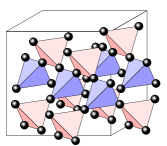
Figure 1: (color online). The network of corner sharing regular tetrahedra formed by the rare earth atoms in the pyrochlore structure in which Er₂Ti₂O₇ crystallizes. The axis of trigonal symmetry at the position of a rare earth is one of the cube diagonals. There are two types of tetrahedra in the network, which differ by their orientation: type B is rotated by 90^∘ about the cubic axes with respect to type A. We distinguish the two sets by two colors in the drawing. Since each rare earth is at a corner shared by two tetrahedra, one of each kind, either the set of the four corners of all the A tetrahedra or the set of the four corners of all the B tetrahedra is sufficient to describe the Er³⁺ lattice.

A single tetrahedron with four Er sites comprises the primitive unit cell. The Er³⁺ crystal sites are all equivalent and the local symmetry is $D_{3d}$, where the 3-fold axes pass through the center of a tetrahedron, in the directions $[111]$, $[\bar{1}\bar{1}1]$, $[\bar{1}1\bar{1}]$ and $[1\bar{1}\bar{1}]$ for the four sites numbered 1, 2, 3, and 4, respectively on a single tetrahedron. According to Hund’s rules, the total angular momentum of the Er³⁺ ion in its ground multiplet is $J=15/2$. The 16-fold degeneracy is lifted into Kramers doublets by the crystal electric field (CEF).

The ground state doublet can be described as an effective spin $S=1/2$ with a quantization axis $z$ parallel to the local trigonal axis. It is well isolated from the excited doublets, the lowest being at about 74 K above the ground state in temperature units.Champion et al. (2003) We shall write the CEF ground state doublet wavefunctions as $|\phi_{0}^{\pm}\rangle$. This doublet is characterized by its spectroscopic factors along and perpendicular to the trigonal axis, $g_{\parallel}$ and $g_{\perp}$ respectively. From a global analysis of the CEF for the pyrochlore $R_{2}$Ti₂O₇ series it has been deduced that $g_{\parallel}=2g_{J}|\langle\phi_{0}^{\pm}|J_{z}|\phi_{0}^{\pm}\rangle|=1.8\,(5)$ and $g_{\perp}=g_{J}|\langle\phi_{0}^{\pm}|J_{\pm}|\phi_{0}^{\mp}\rangle|=7.7\,(1)$.Bertin et al. (2012) Here $g_{J}=6/5$ is the Landé factor. These spectroscopic factors are related to matrix elements that we shall need for the analysis of neutron scattering data. We have

$$j_{\rm CEF} \equiv \langle\phi_{0}^{+}|J_{z}|\phi_{0}^{+}\rangle=-\langle\phi_{0}^{-}|J_{z}|\phi_{0}^{-}\rangle=0.75\,(20),$$ (1)

$$t_{\rm CEF} \equiv \langle\phi_{0}^{\pm}|J_{\pm}|\phi_{0}^{\mp}\rangle=6.42\,(8).$$ (2)

where $J_{\pm}\equiv J_{x}\pm iJ_{y}$. The matrix elements obviously refer to quantities written in local axes; see Appendix A.1 for a discussion. By definition, the large difference between $j_{\rm CEF}$ and $t_{\rm CEF}$ (and obviously also between $g_{\parallel}$ and $g_{\perp}$) reflects the strong CEF anisotropy of the XY type of the Er spins (in contrast to the Ising limit for which $j_{\rm CEF}\gg t_{\rm CEF}$).

The compound displays a magnetic phase transition at $T_{\rm N}\simeq 1.2$ K.Blöte et al. (1969) The large negative value of the Curie-Weiss temperature $\theta_{\rm CW}$ ($\theta_{\rm CW}=-22$ K is deduced from susceptibility data measured between 20 and 50 K; see Refs. Blöte et al., 1969; Bramwell et al., 2000) suggests a strong antiferromagnet coupling.

Neutron diffraction shows the magnetic structure below $T_{\rm N}$ to be noncollinear with the propagation vector ${\bf k}=(0,0,0)$.Champion et al. (2003) From polarized neutron diffraction, the Er³⁺ magnetic moment is determined to be $m=3.25\,(9)\,\mu_{\rm B}$ at low temperature.Poole et al. (2007) A note of caution seems justified at this juncture: $m$ is not directly related to the spectroscopic factors which have been determined for a paramagnetic ion, since the molecular field has to be taken into account for an estimation of $m$. The diffraction data have been originally described Champion et al. (2003); Poole et al. (2007) with the $\Gamma_{3}^{+}$ irreducible representation. We notice that this description also considered in Refs. Ruff et al., 2008; Cao et al., 2010; Sosin et al., 2010 has been recently disputed by Briffa et al.Briffa et al. (2011)

In fact the available microscopic information provides an insight into the moment orientation. Let us consider a one-half spin subjected to a molecular field oriented at a polar angle $\theta$ from the [111] axis. The following relation can be derived:Abragam and Bleaney (1970); Bonville et al. (1978)

$$\tan\theta={g_{\parallel}\over g_{\perp}}\sqrt{{\mu^{2}_{\rm B}g^{2}_{\parallel}-4m^{2}\over 4m^{2}-\mu^{2}_{\rm B}g^{2}_{\perp}}}.$$ (3)

Numerically this gives $\theta\approx 20^{\circ}$. This means that the field is not far from being parallel to the [111] axis. However, the polar angle $\phi$ of ${\bf m}$ is given by $\tan\phi=(g_{\perp}/g_{\parallel})^{2}\tan\theta$, i.e. $\phi\approx 80^{\circ}$. Taking into account the uncertainties on $g_{\perp}$, $g_{\parallel}$, and $m$, this analysis indicates that the moment is perpendicular to the local [111] axis, or at least close to being perpendicular. This is consistent with the magnetic structure first proposed by Champion et al.,Champion et al. (2003) and invalidates the proposal of Ref. Briffa et al., 2011.

Regardless of the magnetic structure, the (2,2,0) Bragg reflection has been shown to be anomalous with broad tails.Ruff et al. (2008) Quantitatively, we find that the intensity around this position is proportional to $|q-q_{(2,2,0)}|^{-\eta}$ with $\eta\simeq 0.6$ for $|q-q_{(2,2,0)}|>0.03$ Å^-1; see Fig. 2.

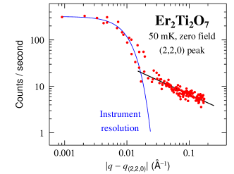
Figure 2: (color online) Neutron intensity for the (2,2,0) Bragg peak of Er₂Ti₂O₇ plotted as a function of $|q-q_{(2,2,0)}|$. The data are from Ruff et al.Ruff et al. (2008) The instrumental resolution is determined from the reflection measured under a 3 T magnetic field. The line for $|q-q_{(2,2,0)}|\geq 0.015$ Å^-1 is described in the main text.

The value of the exponent $\eta$ is much reduced compared to $\eta\simeq 1.8$ found in Tb₂Sn₂O₇.Dalmas de Réotier et al. (2006); Chapuis et al. (2007) For a conventional ordered compound the neutron intensity would be Gaussian-like, i.e. with a much steeper slope.

Inelastic neutron scattering data recorded in zero field suggest the presence of magnetic soft modes,Ruff et al. (2008) in agreement with the power law behavior of the specific heat below $T_{\rm N}$.Sosin et al. (2010) At first sight this is surprising given the expected strong crystal-field anisotropy of the Er³⁺ ions.Briffa et al. (2011)

III Experimental

Er₂Ti₂O₇ single crystals were grown by the floating zone technique using a commercial optical furnace. Feed rods were prepared from high purity oxides (TiO₂, 99.995% and Er₂O₃, 99.99%), mixed and heat treated up to 1180^∘C. After sintering, a rod was heat treated up to 1350^∘C in air. Crystal growth conditions were optimized under air (1 $\ell$/mn) at the growth rate of 2 mm/h coupled with a rotation rate of 30 rounds per minute. As with most of the titanate pyrochlores, Er₂Ti₂O₇ crystallized rods are mostly transparent, with a slight pink color. No phases other than the cubic one with $Fd\bar{3}m$ space group were detected by x-ray powder diffraction experiments; see Fig. 3

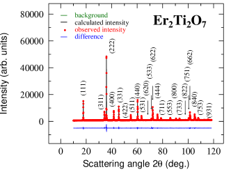
Figure 3: (color online). An example of an x-ray diffraction pattern recorded at room temperature for an Er₂Ti₂O₇ powder obtained after crushing part of a crystal. The radiation used is Co K_α. The line at the bottom of the graph shows the difference between the data and the refinement model.

for an example. As grown and post growth heat-treated crystals were characterized by specific heat measurements. No noticeable differences were detected; see Fig. 4.

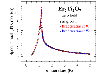
Figure 4: (color online). Specific heat versus temperature for three samples cut from an Er₂Ti₂O₇ crystal prepared as indicated in the main text. For the first sample, no subsequent treatment has been performed, while the other two result from post-growth heat treatments as follows. Case #1: heat treatment for 7 days under oxygen at 1150^∘C, followed by a slow cooling down to 400^∘C. Case #2: heat treatment for 7 days under argon at 1150^∘C, followed by a slow cooling down to 400^∘C.

This is in contrast to the case of Tb₂Ti₂O₇.Yaouanc et al. (2011) The position of the peak provides a measure of the critical temperature. We get $T_{\rm N}=1.23\,(1)$ K. For comparison the following values have already been published: $1.25$ K (Ref. Blöte et al., 1969) and $1.173\,(2)$ K (Ref. Champion et al., 2003) in reasonable agreement.

The investigation of the macroscopic properties of the system consisted of magnetic susceptibility experiments performed with a commercial magnetometer (Magnetic Property Measurement System, Quantum Design inc.) down to 2 K, and of heat capacity measurements. For this latter physical property, the temperature range from 0.48 to 20 K was investigated with a commercial calorimeter (Physical Property Measurement System, (PPMS) Quantum Design inc.) equipped with a ³He stage using a standard thermal relaxation method. Additional measurements between 0.11 and 2.50 K were performed with a home-made calorimeter inserted in a dilution refrigerator using a semi-adiabatic technique.

The $\mu$SR measurements were carried out at the European Muon Spectrometer of the ISIS facility (Rutherford Appleton Laboratory, United Kingdom) and the Low Temperature Facility of the Swiss Muon Source (S$\mu$S, Paul Scherrer Institute, Switzerland). The muon beam is pulsed at the former facility and pseudo-continuous at the latter.

The neutron scattering experiments were performed at the Institut Laue Langevin (ILL, Grenoble) with the lifting-counter diffractometer D23 of the CEA collaborating Research Group (CRG).

IV Bulk measurements

Here we shall first discuss magnetic susceptibility measurements. Then we shall present zero-field specific heat results and finish with the determination of the magnetic phase diagram using specific heat-data recorded under magnetic fields.

IV.1 Magnetic susceptibility

Since the magnetization measurements were performed on a needle-shape sample and the field was applied along its long axis, the demagnetization field is negligible.

Classically, the static magnetic susceptibility $\chi$ is expected to follow a Curie-Weiss law far from the ordering temperature in the paramagnetic regime. It reads

$$\chi={C\over T-\theta_{\rm CW}},$$ (4)

where the Curie constant $C$ can be expressed in terms of the so-called paramagnetic moment $m_{\rm para}$:

$$C={1\over v}{\mu_{0}\,m^{2}_{\rm para}\over 3k_{\rm B}},$$ (5)

where $v=a^{3}/N_{\rm cell}$ with $N_{\rm cell}$ being the number of Er³⁺ ions in the cubic cell ($N_{\rm cell}=16$). For an isolated Er³⁺ ion, $m_{\rm para}=g_{J}\sqrt{J(J+1)}\,\mu_{\rm B}=9.58\,\mu_{\rm B}$.

In Fig. 5 we display our result for the inverse of the static susceptibility versus temperature in a large temperature range. The Curie-Weiss law provides a good description of our data above 30 K. The fit gives for the Curie-Weiss temperature $\theta_{\rm CW}=-17.5\,(3)$ K and $C=3.73\,(4)$ K. This means that $m_{\rm para}=9.55\,(10)\,\mu_{\rm B}$, in agreement with the result for an isolated Er³⁺ ion. Because $\theta_{\rm CW}$ is negative, the dominant exchange interactions are antiferromagnetic.

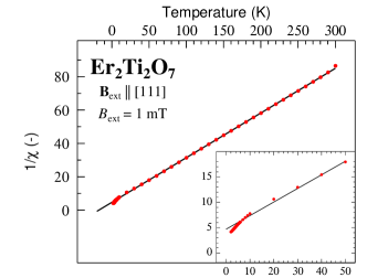
Figure 5: (color online) Inverse of the magnetic susceptibility of an Er₂Ti₂O₇ crystal versus temperature in a large temperature range. The solid line results from a fit with the Curie-Weiss law. A field of 1 mT is applied along a diagonal of the cubic crystal structure. The inset shows the low temperature range of the data.

For comparison, fitting data recorded between 20 and 50 K on a powder sample in a field of 1 mT, Bramwell et al.Bramwell et al. (2000) found values of $\theta_{\rm CW}=-22.3\,(3)$ K and $m_{\rm para}=9.34\,(9)\,\mu_{\rm B}$, For data recorded between 50 and 300 K in a field of 50 mT these authors obtain $\theta_{\rm CW}=-15.93\,(3)$ K and $m_{\rm para}=8.936\,(4)\,\mu_{\rm B}$, the latter at variance with the result for an isolated Er³⁺ ion. From our result, we compute for the frustration indexRamirez (2001) $f\equiv|\theta_{\rm CW}|/T_{\rm N}=14$. Since $f\gg 1$, Er₂Ti₂O₇ is a strongly frustrated magnet. In addition, assuming the Er³⁺ magnetic moments to interact through a simple nearest-neighbor Heisenberg interaction with exchange integral ${\mathcal{I}}$ (${\mathcal{I}}>0$), i.e.

$${\mathcal{H}}={{\mathcal{I}}\over 2}\sum_{i,j,i\neq j}{\bf J}_{i}\cdot{\bf J}_{j}={\mathcal{I}}\sum_{\langle i,j\rangle}{\bf J}_{i}\cdot{\bf J}_{j},$$ (6)

the molecular-field approximation predicts

$${\mathcal{I}}={3\,k_{\rm B}|\theta_{\rm CW}|\over z_{\rm nn}J(J+1)}.$$ (7)

We denote as $z_{\rm nn}$ the number of nearest neighbor Er³⁺ ions to a given Er³⁺ ion. In our case $z_{\rm nn}$ = 6. From the measured $\theta_{\rm CW}$ value and taking into account that $J=15/2$, we compute ${\mathcal{I}}/k_{\rm B}=0.138\,(2)$ K.

We have also measured the susceptibility for $2.0<T<6.0$ K under a field of 1 mT applied along a $[111]$ axis using two protocols; see Fig. 6. Contrary to a previous report,Bramwell et al. (2000) we do not observe any history dependent effect at $T\leq 3.2$ K. Hence, there is no spin-glass-like irreversible effect for our Er₂Ti₂O₇ crystals.

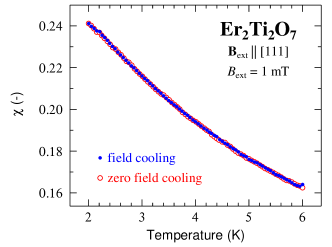
Figure 6: (color online) The magnetic susceptibility of an Er₂Ti₂O₇ crystal versus temperature in the low temperature region. The same magnetic response is observed using either the field or zero-field cooling procedure, fc and zfc respectively. A field of 1 mT is applied along a diagonal of the cubic crystal structure. In the zfc mode the sample was warmed to 300 K and then cooled to 2 K before applying the magnetic field. In the fc mode the field was applied at 300 K and the sample was subsequently cooled down.

IV.2 Specific heat in zero magnetic field

Here we present and discuss zero-field specific heat data recorded for Er₂Ti₂O₇ crystals. It is well known that they may lead to a characterization of the low energy magnetic modes, detect indirectly a dynamical magnetic component in the ordered state, determine the universality class of the system under study, and gauge a possible residual entropy at low temperature.

In Fig. 7 we display our data, in the low temperature regime.

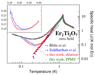
Figure 7: (color online) Low temperature specific heat of Er₂Ti₂O₇. The open symbols show our experimental data compared to literature results from Blöte et al.Blöte et al. (1969) and Siddharthan et al.Siddharthan et al. (1999) Note the large overlap between our results obtained with the PPMS and the home-made calorimeter inserted in a dilution refrigerator. The filled symbols present the electronic specific heat deduced from the data of Siddharthan et al. and this work. The dashed lines show the contributions from the nuclear specific heat and the full line results from a fit of the low temperature electronic specific heat to the $C_{\rm elec}={\mathcal{B}}T^{3}$ law, with $\mathcal{B}$ = 2.50 (15) J K^-4 mol^-1. The inset displays the very low temperature details. The solid lines result from fits as explained in the main text.

While our results are in reasonable agreement with data published by Siddharthan et al.,Siddharthan et al. (1999) they differ drastically at low temperature with the ones of Blöte et al.Blöte et al. (1969) We do not understand the origin of the large difference with the data of Blöte et al. In the following we shall focus on the analysis of our data and the ones of Siddharthan et al. Note that here we have not considered the results of Sosin et al.Sosin et al. (2010) since they do not extend to very low temperature.

In the low temperature range shown in Fig. 7 the specific heat arises from three origins: the contribution from the nuclei with non-zero spins at low temperature, then the low energy magnon modes at higher temperature and the critical fluctuations around $T_{\rm N}$. As a start we shall focus on the first two contributions, i.e. the specific heat of nuclear and magnon origins, $C_{\rm n}$ and $C_{\rm sw}$, respectively.

We begin with providing a theoretical background for these contributions, focusing first on the nuclear one. $C_{\rm n}$ arises from the ¹⁶⁷Er nuclear magnetic moments (¹⁶⁷Er is the only non-spinless isotope of Er with 23% natural abundance), since the contribution of the two Ti isotopes is negligible, as in the case of Tb₂Ti₂O₇.Yaouanc et al. (2011) Contrary to Tb₂Ti₂O₇ the quadrupole interaction is not negligible compared to the Zeeman interaction. This is due to the fact that the quadrupole moment $Q_{167}$ of ¹⁶⁷Er is larger than that of ¹⁵⁹Tb (3.565 vs 1.432 barns) and the gyromagnetic ratio $\gamma_{167}$ of ¹⁶⁷Er is much smaller, in absolute value, than that of ¹⁵⁹Tb ($-7.7157$ vs 64.31 Mrad s^-1 T^-1); see Ref. Harris et al., 2001. The Zeeman and quadrupolar Hamiltonians are written

$${\mathcal{H}}_{{\rm Zee}} = -\hbar\gamma_{167}{\bf I}\cdot{\bf B}_{\rm hyp}$$ (8)

and

$${\mathcal{H}}_{{\rm Q}} = \hbar\omega_{\rm Q}\left[3I_{z}^{2}-I(I+1)\right],$$ (9)

respectively. In these equations, ${\bf I}$ is the ¹⁶⁷Er spin operator ($I$ = 7/2) and $\hbar\omega_{\rm Q}$ = ${eQ_{167}V_{zz}\over 4I\left(2I-1\right)}$ where $V_{zz}$ is the principal component of the electric field gradient tensor acting on the rare earth nucleus with $z$ being as before the local three-fold axis. The symmetry at the rare earth site imposes the electric-field gradient to be axial. Because the Er³⁺ ordered magnetic moments are (nearly) perpendicular to $z$ we shall also take ${\bf B}_{\rm hyp}$ perpendicular to this axis. As usual $\hbar$ and $e$ stand for the Dirac constant and the proton electric charge, respectively.

The nuclear energy levels are determined after diagonalization of the Hamiltonian ${\mathcal{H}}_{\rm n}$ = ${\mathcal{H}}_{{\rm Zee}}+{\mathcal{H}}_{{\rm Q}}$ and $C_{\rm n}$ is readily obtained. ${\mathcal{H}}_{\rm n}$ depends on two parameters, $B_{\rm hyp}$ and $V_{zz}$. While an estimate for $V_{zz}$ is provided in Appendix B, $B_{\rm hyp}$ will be a fitting parameter.

The other contribution to the low temperature specific heat arises from magnons. Low energy magnons have indeed been observed in neutron scattering experiments.Ruff et al. (2008) The dispersion relation $\hbar\omega({\bf q})$ for their lowest energy branch is needed to compute $C_{\rm sw}$. An approximate expression valid at small wavevectors is

$$\hbar^{2}\omega^{2}({\bf q})=\hbar^{2}\omega^{2}(q)=\Delta^{2}_{\rm sw}+\hbar^{2}v_{\rm sw}^{2}q^{2}.$$ (10)

Here $\Delta_{\rm sw}$ is the gap energy of the magnon spectrum at the zone center and $v_{\rm sw}$ is the magnon velocity. We note that a dispersion relation has recently been proposed for Er₂Ti₂O₇ in the framework of linear spin-wave theory.Savary et al. (2012) The applicability of this theory in frustrated systems might be questionable as recently discussed in the case of the triangular lattice.Zheng et al. (2006) Still, the model of Ref. Savary et al., 2012 leads to an anisotropic dispersion relation. The resulting specific heat depends on a single magnon velocity which is the geometrical mean of the three magnon velocities along orthogonal axes. In our model it corresponds to $v_{\rm sw}$.

When $\Delta_{\rm sw}$ is negligible, the magnon specific heat $C_{\rm sw}$ can be computed in the temperature range where only small wavevectors are at play, i.e. when Eq. 10 applies. The expected $T^{3}$ law for $C_{\rm sw}$ is derived:

$$C_{\rm sw}={\mathcal{A}}T^{3}\ \ {\rm with}\ \ {\mathcal{A}}={\pi^{2}\over 120}{\mathcal{N}}_{\rm A}{k^{4}_{\rm B}a^{3}\over\hbar^{3}v^{3}_{\rm sw}},$$ (11)

where ${\mathcal{N}}_{\rm A}$ is Avogadro’s constant. This result only holds at sufficiently low temperature.

Having established the theoretical background, we now perform the specific heat data analysis. We shall do it in two steps.

We first attempt to determine whether a $T^{3}$ behavior can be observed. A fit to the measured specific heat at the lowest temperatures for which the magnon contribution should be negligible enables us to estimate $C_{\rm n}(T)$ and then to subtract it from the measured heat capacity. The resulting electronic heat capacity, $C_{\rm elec}$, is presented in the main panel of Fig. 7 for our data and the ones of Siddharthan et al. It follows nicely a $T^{3}$ law in a restricted temperature range, but deviates above $\approx T_{\rm N}/2.5$, in contrast to published results.Champion et al. (2003); Sosin et al. (2010) This observation justifies to identify $C_{\rm elec}$ with $C_{\rm sw}$. The $T^{3}$ behavior is not expected to be seen at low temperature if the energy gap is appreciable. The effect of the gap might be seen around $T=0.2$ K; see Fig. 7. However, $C_{\rm elec}$ becomes very small at that temperature and difficult to measure as reflected by the distribution of the $C_{\rm elec}$ data. Hence, we cannot determine whether a gap is present from this plot. Numerically, since we can identify ${\mathcal{B}}$ given in the caption of Fig. 7 with ${\mathcal{A}}$ of Eq. 11, we get $v_{\rm sw}$ = 86 (2) m s^-1.

The second step for the interpretation of the specific heat data consists in fitting the measured specific heat to the sum $C_{\rm n}+C_{\rm sw}$. This sum depends on three parameters, $\Delta_{\rm sw}$, $v_{\rm sw}$ and $B_{\rm hyp}$. The fit is shown in the inset of Fig. 7. Its temperature range is restricted on the high temperature side because of the requirement that only the low energy magnons determine the value of the integral. Two solid lines are drawn in the figure since the two data sets are slightly different at low temperature. Both sets can be fit to a range of gaps extending from nearly zero to an upper bound. We find $\Delta_{\rm sw}/k_{\rm B}\leq$ 0.5 (1) K for both data sets. This is consistent with the value of Sosin et al.Sosin et al. (2010) We also derive $v_{\rm sw}$ = 84 (2) and 82 (2) m s^-1 and $B_{\rm hyp}$ = 345 (10) and 305 (5) T for the Siddharthan et al. data and our data, respectively. Note that $B_{\rm hyp}$ depends very little on the actual value chosen for $V_{zz}$.

We now discuss these results, starting with the bound on the spin gap energy. This bound is really small and might be surprising at a first sight given the strong magnetic anisotropy of Er₂Ti₂O₇. However, the Er³⁺ magnetic moment lies at a polar angle of nearly 90^∘ with respect to the local three-fold axis. This angle is imposed by the relatively strong crystal field interaction. There is still a continuous degree of freedom for the azimuthal angle. The magnetic order breaks this rotational symmetry and $\Delta_{\rm sw}$ is a measure of the residual anisotropy energy. We note that the upper bound value for $\Delta_{\rm sw}$ is in the expected range if it arises from the dipole interaction between the Er³⁺ magnetic moments.

We examine now the magnon velocity value and tentatively relate it with the exchange integral introduced in Eq. 6. For this purpose we resort to the phenomenological dispersion relation

$$\hbar^{2}\omega^{2}({\bf q})=\hbar^{2}\omega^{2}(q)=\Delta^{2}_{\rm sw}+\left[{\mathcal{I}}z_{\rm nn}J\sin(qd)\right]^{2},$$ (12)

where $d$ is the distance between two magnetic atoms. In fact, had we written $\sin(q^{Z}d)$ instead of $\sin(qd)$, Eq. 12 would give the dispersion relation of an antiferromagnetic chain running along the $Z$ direction and of lattice parameter $d$ for which the number of nearest neighbors is $z_{\rm nn}=2$; see for example Ref. Lovesey, 1986. Here we shall take $d$ as the distance between two Er atoms, i.e. $d=a/(2\sqrt{2})$. Identifying the small $q$ expansion of Eq. 12 with Eq. 10 we have

$$v_{\rm sw}={15\over 2\sqrt{2}}a{{\mathcal{I}}\over\hbar},$$ (13)

using $J=15/2$. This relation leads to ${\mathcal{I}}/k_{\rm B}$ = 0.118 (4) K, a value in reasonable agreement with the one derived from the Curie-Weiss constant; see Sec. IV.1. We shall return to the interpretation of the magnon velocity at the end of Sec. V.2 once a nearest neighbor Hamiltonian consistent with the symmetry of the lattice has been introduced.

It is possible to get interesting information from the $B_{\rm hyp}$ values. Using the hyperfine constant which is $87\,(1)\,{\rm T}/\mu_{\rm B}$,Ryan et al. (2003) the magnetic moment at the origin at the field can be obtained. We derive for the moment $4.0\,(2)$ and $3.5\,(1)\,\mu_{\rm B}$ from the Siddharthan et al. measurement and ours, respectively. The latter value is consistent with the neutron result.Poole et al. (2007) Hence, contrary to Tb₂Sn₂O₇ (Ref. Bonville, 2010) there is no reduction of the hyperfine field at the ¹⁶⁷Er nuclei due to electronic spin dynamics. This means that the characteristic time for the electronic spin-flip is substantially larger than the ¹⁶⁷Er spin-lattice relaxation time.Bertin et al. (2002)

We now turn our attention to the critical behavior of the specific heat in the paramagnetic phase. In Fig. 8 we display our data using a reduced temperature scale. We expect to observe the usual power law critical behavior:Fisher (1964); Kornblit and Ahlers (1973)

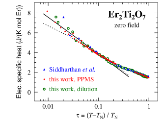
Figure 8: (color online) Zero-field specific heat of Er₂Ti₂O₇ versus the reduced temperature parameter $\tau$ in the paramagnetic regime for three data sets. The full (dotted) line is the prediction of Eq. 14 for $\alpha$ = $-0.015$ ($-0.134$). For $\alpha$ = $-0.015$ we find $C_{\rm sh}$ = 1.7 (1) J K^-1 mol^-1. The critical regime is observed up to $\tau$ $\simeq 0.2$.

$$C_{\rm elec}(T)=\frac{C_{\rm sh}}{\alpha}\left[\left({T-T_{\rm N}\over T_{\rm N}}\right)^{-\alpha}-1\right],$$ (14)

where $C_{\rm sh}$ is a constant and $\alpha$ the specific heat critical exponent. By definition, $C_{\rm elec}(T)$ has a maximum at $T_{\rm N}$. This enables us to determine $T_{\rm N}$, as already mentioned in Sec. III. The exponent $\alpha$ is expected to be $\alpha=-0.015$ and $-0.134$ for the three-dimensional XY and Heisenberg magnets, respectively. As seen in Fig. 8, Eq. 14 provides a better account of the data for the XY case, as expected.

Before leaving this section, we discuss the entropy variation of our system using our specific heat results. We have extended the specific heat measurement $C_{\rm p}$ of Er₂Ti₂O₇ up to approximately 20 K and measured the specific heat of the isostructural non-magnetic compound Y₂Ti₂O₇ in the same temperature range. The sum of the contributions from the nuclear moments and the lattice, the latter being estimated from scaling the Y₂Ti₂O₇ result,Chapuis et al. (2010) is presented in the inset of Fig. 9, as well as $C_{\rm p}(T)$. The resulting $C_{\rm elec}(T)$ obtained from subtracting the contributions of the nuclear moments and the lattice to $C_{\rm p}(T)$ is displayed in the main frame of Fig. 9.

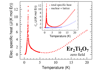
Figure 9: (color online) The electronic specific heat of Er₂Ti₂O₇ in an extended temperature range. In the inset are displayed the total specific heat ($C_{\rm p}$) of Er₂Ti₂O₇ and the sum of the estimated nuclear and lattice contributions.

In Fig. 10 we present $\Delta S_{\rm elec}(T)$, which is the temperature variation of the electronic entropy obtained by integrating $C_{\rm elec}(T^{\prime})/T^{\prime}$ from $0.115$ K, the lowest measured temperature, to the temperature of interest $T$.

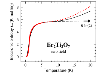
Figure 10: (color online) The variation of the electronic entropy $\Delta S_{\rm elec}(T)$ of Er₂Ti₂O₇ versus temperature $T$. The solid line is computed assuming two singlet states at energies corresponding to 0 and 2.85 K and two doublets at 74 and 85.8 K. A signature of the two doublets has been seen by inelastic neutron scattering.Champion et al. (2003) The ground state doublet has been split to account for the magnetic order of Er₂Ti₂O₇ below $T_{\rm N}$, with the splitting taken as a fitting parameter. Admittedly, this is a very rough description of the physics. The dashed line is the result of the computation of $\Delta S_{\rm elec}(T)$ when only the first two levels are taken into account.

Remarkably, $\Delta S_{\rm elec}(T)$ reaches the $R\ln(2)$ value at approximately 8 K. This is the entropy variation expected for an isolated doublet state. Therefore the residual entropy left as $T\rightarrow 0$ is extremely small if any. For temperatures above 8 K, $\Delta S_{\rm elec}(T)$ keeps increasing owing to the contribution of the excited CEF levels. This is clearly shown in Fig. 10, where a comparison is made between the results of computations of $\Delta S_{\rm elec}(T)$ either taking into account the first excited CEF levels or neglecting them.

IV.3 Specific heat under an external magnetic field

We have constructed the phase diagram of Er₂Ti₂O₇ in the field-temperature plane using specific heat data. Examples of measurements are shown in Fig. 11.

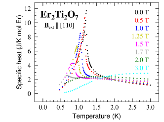
Figure 11: (color online) Temperature dependence of the specific heat of a Er₂Ti₂O₇ single crystal for different magnetic field intensities applied along $[110]$. The maximum of the specific heat peak moves to lower temperatures as the field increases up to 1.7 T. No peak is observed when the field strength is above 1.7 T.

For a given external field we have determined the temperature at which the specific heat displays a maximum. The position of the maximum as a function of the field intensity for a given field orientation relative to the crystal axes is displayed in Fig. 12.

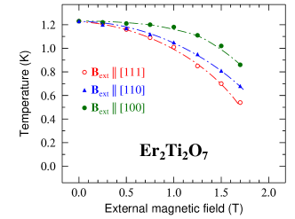
Figure 12: (color online) The phase diagram derived from specific heat measurements for the three main crystal directions of cubic Er₂Ti₂O₇. The dashed-dotted lines are guides to the eye.

Our results are consistent with the ones already published,Ruff et al. (2008); Sosin et al. (2010) but only qualitatively. Note that here we establish the phase diagram for the three main directions of a cubic compound. These data suggest a quantum critical point to be present slightly above 2 T and to be dependent on the field orientation.

V Microscopic technique measurements

Single crystals of Er₂Ti₂O₇ have been studied by two microscopic experimental techniques: positive muon spin relaxation ($\mu$SR) and neutron scattering. We shall first discuss the $\mu$SR results.

V.1 $\mu$SR

In the longitudinal geometry that we have used, a $\mu$SR spectrum recorded in the magnetically ordered state of a crystal is expected to display either (i) at least one damped oscillation if the initial muon beam polarization is not parallel to the spontaneous field at the muon site, or (ii) a missing fraction if the oscillation cannot be resolved.Yaouanc and Dalmas de Réotier (2011) None of these two possibilities was observed at ISIS or S$\mu$S. The zero-field spectrum recorded at 21 mK is displayed in Fig. 13; the spectral shape shows little change up to $\approx$ 0.5 K. The same type of spectra was also observed for different orientations of the initial muon beam polarization relative to the crystal axes. Hence, the absence of oscillation cannot be attributed to the initial muon beam polarization which would be parallel to the internal field. This situation would moreover be unexpected because of the four equivalent symmetry $\langle 111\rangle$ axes at the Er³⁺ site. In addition to the absence of oscillation, the shape of the zero-field spectra is extremely unusual. Indeed, the spectral slope is quasi-constant up to $\approx$ 0.4 $\mu$s, then it increases and eventually monotonically decreases above $\approx$ 0.7 $\mu$s. This kind of behavior drastically differs from the usual relaxation spectra, which are characterized by a monotonically decreasing slope, as e.g. in the common exponential relaxation. It does not either remind the shape of spectra associated with a static or quasistatic field distribution at the muon. At this stage we cannot actually conclude whether the spectral shape is mainly influenced by a static field distribution or dynamical effects. We shall come back to this point when commenting the data recorded in applied fields.

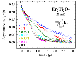
Figure 13: (color online) $\mu$SR spectra of a Er₂Ti₂O₇ crystal taken at S$\mu$S with the initial muon beam polarization parallel to the $[111]$ crystal direction. The spectra were recorded in zero and various longitudinal fields as indicated in the figure.

Since no spontaneous muon precession is observed, it is tempting to make an analogy with Tb₂Sn₂O₇ for which there is also no detected oscillation in the magnetically ordered state.Dalmas de Réotier et al. (2006) This analogy would be completely justified if the zero-field spectrum was exponential. However, we have just remarked that it is obviously not the case. It is not Gaussian either, as first suggested.Lago et al. (2005) A close look at the data in Ref. Lago et al., 2005 shows that the zero-field relaxation is in fact consistent with the one we observe.

Before discussing further the significance of our result, it is worthwhile to consider the longitudinal field spectra shown in Fig. 13. First note that with the considered field intensities the compound has a priori not crossed the phase diagram boundary displayed in Fig. 12. While the application of fields below 0.5 T has little influence on the spectral shape, it is not the case for higher fields. Interestingly, for the highest fields shown in the figure, the spectra tend to be described by an exponential function. This implies that the muon repolarization is not at the origin of the field dependence of the spectra and that dynamics is mainly influencing the muon response in Er₂Ti₂O₇. The time scale of this dynamics can be roughly estimated. For this purpose we have recourse to the Lorentzian field dependence of the exponential relaxation rate $\lambda_{Z}$ in the motional narrowing, i.e. fast fluctuation limit.Redfield (1957); Yaouanc and Dalmas de Réotier (2011) In this model the relaxation rate in a field $B_{\rm ext}$ is such that $\lambda_{Z}(B_{\rm ext})/\lambda_{Z}(B_{\rm ext}=0)$ = 1/2 for $B_{\rm ext}$ = $B_{1/2}$ = $1/(\gamma_{\mu}\tau_{\rm f})$. Here $\tau_{\rm f}$ is the fluctuation time of the spins and $\gamma_{\mu}=851.615\,{\rm Mrad}\,{\rm s}^{-1}\,{\rm T}^{-1}$ is the muon gyromagnetic ratio. Taking 1 T as an order of magnitude for $B_{1/2}$ we find $\tau_{\rm f}\approx 10^{-9}$ s.

We have therefore established that the muons are probing dynamical fields. No oscillation is detected in zero-field because the mean field at the muon site does not keep a constant value for a time sufficiently long for a muon spin precession to be observed.Dalmas de Réotier et al. (2006) We denote this field as ${\bf B}_{\rm fluc}$. It arises from the dipole interaction of the muon magnetic moment with the Er³⁺ magnetic moments. Given the size of the Er³⁺ magnetic moment, we estimate $B_{\rm fluc}$ in the range 0.1-0.2 T.

With our knowledge for $\tau_{\rm f}$ and $B_{\rm fluc}$, we find $\tau_{\rm f}\gamma_{\mu}B_{\rm fluc}=B_{\rm fluc}/B_{\rm ext}\ll 1$. For the simple model of ${\bf B}_{\rm fluc}$ flipping from parallel to antiparallel to an axis perpendicular to initial muon polarization ${\bf S}_{\mu}$, we would expect the zero-field relaxation to be exponential,Yaouanc and Dalmas de Réotier (2011) as found for Tb₂Sn₂O₇. However, experimentally this is not the case. This is not surprising given the fact that the magnetic diffraction profiles are complex. Their shape is ascribed to the coexistence of long and short-range dynamical correlations; see our discussion of Fig. 2. To the distribution of correlation lengths must correspond distributions of spin-spin and spin-lattice relaxation rates. This may explain the exotic shape of the zero-field $\mu$SR relaxation function.

Relative to Tb₂Sn₂O₇, the fluctuations probed by $\mu$SR in Er₂Ti₂O₇ are slower by roughly an order of magnitude. From neutron spin-echo measurements it is known that in the ordered state of Tb₂Sn₂O₇ spin correlations near the zone center are staticChapuis et al. (2007) within the technique time scale, while they are dynamical in nature far outside the center of the zone.Rule et al. (2009) It would be worthwhile to examine the dynamics of the magnetic correlations in Er₂Ti₂O₇ with the neutron spin-echo technique.

From the analysis of the nuclear specific heat in Sec. IV.2, it was inferred that the ratio of $\tau_{\rm f}$ to the nuclear spin-lattice relaxation time was larger in Er₂Ti₂O₇ than in Tb₂Sn₂O₇. Assuming the spin-lattice relaxation times in the two compounds to be similar, the nuclear specific heat data are consistent with the results of the analysis of the $\mu$SR spectra.

V.2 Neutron scattering

Paramagnetic correlations were studied by diffuse neutron scattering in Er₂Ti₂O₇ crystals. Two scattering planes were investigated: $(h,k,0)$ and $(h,k,k)$ at 2.00 (3) and 1.47 (3) K, respectively. For the first (second) one a graphite (copper) monochromator was used delivering neutrons of wavelength 2.377 (1.275) Å. No energy analysis of the scattered beam was performed. In order to deal with magnetic correlations only, additional maps were recorded at 50 K for both geometries and they were subtracted from the corresponding low temperature counterparts. The resulting two maps were divided out by the square modulus of the Er³⁺ magnetic form factor. The effect of the form factor is modest: no more than 20% on the vast majority of the data. The resulting experimental data are displayed in Fig. 14. It is to be noted that the intensities are negative for large regions in the two planes. This reflects the fact that the wavevector independent scattering associated with the CEF states of the Tb³⁺ ions is larger at 50 K than at low temperature.

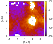
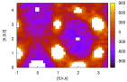
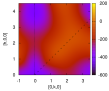
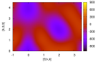
Figure 14: (color online) Top two panels: magnetic diffuse neutron scattering intensity recorded for a crystal of Er₂Ti₂O₇ in the reciprocal $(h,k,0)$ and $(h,k,k)$ planes at 2.00 (3) and 1.47 (3) K respectively. The positions in the reciprocal lattice are in $2\pi/a$ units, where $a$ is the lattice parameter of the cubic unit cell. These maps are obtained as explained in the main text. To preserve the maps appearance, pixels with off scale intensities, e.g pixels influenced by Bragg reflections and critical scattering, as well as pixels located near the origin of the reciprocal lattice have been graphically eliminated: they are represented in white color. Bottom two panels: $(h,k,0)$ and $(h,k,k)$ magnetic correlation maps computed with the tetrahedron model explained in the main text. The comparison between the theoretical and experimental maps displayed above enables us to derive information on the Er₂Ti₂O₇ interaction constants. The lines drawn in the $(h,k,0)$ maps indicate the position of the cuts shown in Fig. 16.

Before attempting a quantitative analysis of the maps, a qualitative discussion is worthwhile. We first note the almost vanishing $(2,2,2)$ spot. This means that the ferromagnetic correlations are negligible. We observe a hexagonal scattering loop in the plane $(h,k,k)$ around the $(2,2,2)$ position. Such a type of scattering is reminiscent of the intensity measured in the cubic spinel ZnCr₂O₄ (Ref. Lee et al., 2002), in which the Cr ions also form a lattice of corner sharing tetrahedra. However, in the latter case the loop is in the plane $(h,k,0)$ and centered around $(2,2,0)$. The scattering properties are therefore quite different for the two compounds. This reflects the difference in magnetic symmetry. The origin of the loops observed in ZnCr₂O₄, which were originally interpreted in terms of weakly interacting hexagonal spin clusters, is now taken as the signature of extended exchange interactions for spin-ice and isotropic systems.Yavors’kii et al. (2008); Conlon and Chalker (2010) In the following we show that the scattering loop in Er₂Ti₂O₇ can basically be taken as a fingerprint of the properties of the exchange interactions within a single tetrahedron.

The discussion of the experimental results will be carried out in two steps. We shall first evaluate the magnetic correlation length at the temperature of the measurements and then analyze the maps using a four-spin Hamiltonian.

V.2.1 Magnetic correlation length

Here we determine the correlation length of the critical magnetic correlations. For this purpose we consider the scattered intensity measured in the vicinity of the reciprocal positions ${\bf q}_{(h,k,l)}$ = ${\bf q}_{(2,2,0)}$ and ${\bf q}_{(1,1,1)}$ at $T=2.00$ and $1.47$ K, respectively; see Fig. 15.

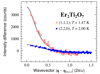
Figure 15: (color online). Magnetic scattering intensity versus wavevector in the vicinity of the two reciprocal lattice positions ${\bf q}_{(h,k,l)}$ where $(h,k,l)$ = (1,1,1) and (2,2,0), respectively. The wavevector unit is $2\pi/a$ where $a$ is the cube edge. The data are obtained from the intensity differences shown in Fig. 14 by averaging the data at reciprocal space points located at equal distance from the two lattice positions. Two requirements were considered when choosing these two positions: they do not lie close to the boundary of the maps and the magnetic intensity is relatively important. The lines are results from fits of Eq. 15 to the data.

This critical scattering intensity is described by the sum of a Lorentzian function and a constant:

$${\mathcal{L}}(|{\bf q}-{\bf q}_{(h,k,l)}|)={I_{\rm L}\over 1+|{\bf q}-{\bf q}_{(h,k,l)}|^{2}/\kappa_{\rm m}^{2}}+I_{0},$$ (15)

where $\kappa_{\rm m}$ is the inverse of the magnetic correlation length. The parameter $I_{\rm L}$ accounts for the magnitude of the Lorentzian, while $I_{0}$ refers to a neutron intensity which is not related to critical scattering. Since at the temperature of experiments, the width of the critical magnetic scattering curve is much larger than the instrumental resolution, the convolution of Eq. 15 by the resolution function is unnecessary. The fits shown in Fig. 15 yield the magnetic correlation lengths $\xi_{\rm m}$ = $\kappa_{\rm m}^{-1}$ = 3.6 (2) and 6.6 (5) Å for the (2,2,0) and (1,1,1) reflections measured at 2.00 and 1.47 K, respectively. As expected, $\xi_{\rm m}$ shoots up as the sample is cooled toward the transition. These two values are comparable with the Er³⁺-Er³⁺ ion distance $d=3.56$ Å. Hence the analysis of the experimental maps shown in Fig. 14 can be performed considering the spin correlations within a single tetrahedron. This is the basis for our quantitative interpretation which is exposed below.

V.2.2 Analysis of the diffuse scattering maps

While our analysis of the magnetic scattering intensity in the vicinity of reciprocal lattice positions at low temperature shows that the measured wavevector dependence probes short-range correlations, a wavevector independent scattering is also observed; see Fig. 15. This scattering reflects local physics, for example of crystal-field nature. Denoting $M({\bf q})$ a measured magnetic scattering map, we write

$$M({\bf q})=S_{\rm shift}+S_{\rm scale}\,N({\bf q}),$$ (16)

where $S_{\rm shift}$ accounts for the wavevector independent scattering, $S_{\rm scale}$ gives the scale of the wavevector dependent magnetic intensity and $N({\bf q})$ is the prediction of our model that we describe now.

In Sec. II we have mentioned that the Er³⁺ crystal-field ground state doublet is well isolated since the first excited doublet is at about $74$ K above the ground state in temperature units. Therefore for low temperature measurements, such as discussed here, it is a reasonable approximation to describe an Er³⁺ ion as an effective $S=1/2$ spin. In Appendix A we discuss the physics of a tetrahedron of effective one-half spins embedded in a pyrochlore lattice. Assuming that only bilinear spin interactions are relevant, the Hamiltonian ${\mathcal{H}}_{\rm t}$ describing the interaction between the four effective spins can be written as a linear combination of four invariants; see Eq. 66. Their weight is gauged by the four parameters $P_{i}$, $i\in\{1,2,3,4\}$.

The wavevector dependent scattering intensity resulting from a single tetrahedron is proportional toLovesey (1986)

$$N({\bf q})=\sum_{m}e^{-E_{m}/(k_{\rm B}T)}f_{m}({\bf q}),$$ (17)

where

$$f_{m}({\bf q})=$$ (18)

$$\sum_{\alpha,\beta}\sum_{i,j}\sum_{n}\left(\delta^{\alpha\beta}-\frac{{q}^{\alpha}{q}^{\beta}}{q^{2}}\right)\langle m|S_{i}^{\alpha}|n\rangle\langle n|S_{j}^{\beta}|m\rangle e^{i{\bf q}\cdot({\bf r}_{j}-{\bf r}_{i})}.$$

The Debye-Waller factor is negligible for the region of the reciprocal space investigated and the temperatures at which the measurements were made. The symbols $\alpha,\beta$ refer to global Cartesian coordinates in the cubic unit cell. The relations between the local and global axes are explicitly given in Appendix A.1. The indices $i$ and $j$ stand for the Er ions at the corners of the tetrahedron, the positions of which are specified by ${\bf r}_{i}$ and ${\bf r}_{j}$, and $|n\rangle$ and $|m\rangle$ refer to two of the sixteen single tetrahedron states, whose energy differences lie within the energy range across which the neutron scattering is integrated. The formula in Eq. 18 does not contain the Er³⁺ form factor since it has already been divided out for the two presented maps.

We have performed a global fit of the two recorded maps. It depends on two $S_{\rm shift}$ parameters, one per map, a unique scale parameter $S_{\rm scale}$ and the four Hamiltonian parameters $P_{i}$. The best fit shown in Fig. 14 is achieved with the following interaction constants in kelvin units:

$$P_{1}/k_{\rm B} =10.4\,(6),\ \ \ P_{2}/k_{\rm B} =-1.2\,(5),$$ (19)

$$P_{3}/k_{\rm B} =3.0\,(3),\ \ \ \ P_{4}/k_{\rm B} =8.4\,(1.3).$$ (20)

The quality of the fit can be assessed from cuts of the experimental and model maps as seen in Fig. 16.

Figure 16: (color online) Cuts of the $(h,k,0)$ maps shown in Fig. 14 along the [1,1,0] and [0,1,0] directions. The circles represent the experimental data and the lines the results of the model. The origin of the horizontal axis is taken at the origin of the reciprocal lattice.

The fitting parameters described above were determined from least square minimization, i.e. minimizing $\chi^{2}$ = $[1/(N_{d}-7)]\sum_{j}(M_{j}-I_{j})^{2}/\sigma_{j}^{2}$ with respect to the fitting parameters. Here $\sigma_{j}$ is the statistical uncertainty on the neutron intensity $I_{j}$ at the $j$th data point in the set of $N_{d}$ data points and $M_{j}$ is the model prediction (a function of the fitting parameters). An uncertainty $\delta P_{i}$ on $P_{i}$ is obtained by varying the neutron intensity by $\partial I_{j}$ at each of a large sample of the data points (one in eight) and minimizing $\chi^{2}$ in order to find the variation of each fitted parameter $\partial P_{i}$. Then $\delta P_{i}$ is estimated using the relation $\delta P_{i}=(1/N_{d})\sqrt{\sum_{j}(\sigma_{j}\partial P_{i}/\partial I_{j})^{2}}$.

We have so far described the estimate of the statistical uncertainties. Three other origins for systematical uncertainties must be considered. First our model describes diffuse scattering and therefore pixels which are sizably influenced by critical scattering should be eliminated in the fitting procedure. For this purpose we have tested the influence of different radius cutoffs around the Bragg points, to the $P_{i}$ values. This cutoff effect introduces the largest parameter uncertainties. Then the temperature at which a map is recorded is known with a finite uncertainty. Finally the uncertainty arising from the error bars on the matrix elements $j_{\rm CEF}$ and $t_{\rm CEF}$ (see Eq. 2) has also been assessed. The error bars given in Eq. 20 account for these statistical and systematical uncertainties.

It is tempting to extract information from the Curie-Weiss constant using the high-temperature susceptibility formula derived Ross et al.Ross et al. (2011) However, this should not be done since that formula depends on spectroscopic factors which provide a description of the physics only at low temperature. A high-temperature expansion for the susceptibility is required to further analyze the data of Fig. 5.

At this juncture it is of interest to mention a recent work by Savary et al. on Er₂Ti₂O₇.Savary et al. (2012) These authors analyze the spin wave dispersions measured for different orientations of the wave vector. The experiments were performed for temperature (30 mK) and field (3 T) values where Er₂Ti₂O₇ is a polarized paramagnet.Ruff et al. (2008) The analysis of the data involves a nearest neighbor Hamiltonian related to ours, with a different definition of the Hamiltonian parameters. Using the relations between the two sets of parameters given in Eq. 73, and assuming $P_{i}$ = $2{\tilde{P}}_{i}$ we find for their parameters in kelvin units,

$$P_{1}/k_{\rm B} =1.74\,(1.26),\ \ \ P_{2}/k_{\rm B} =-0.44\,(74),$$ (21)

$$P_{3}/k_{\rm B} =2.92\,(34),\ \ \ \ \ P_{4}/k_{\rm B} =9.0\,(1.0).$$ (22)

These $P_{2}$, $P_{3}$ and $P_{4}$ values are in very good agreement with ours. However an important difference is observed in $P_{1}$, i.e. the parameter which controls the interaction along the local hard magnetic axis. We have simulated the diffuse scattering intensity obtained from this latter set of parameters and compared it with our experimental data. We obtain an acceptable fit of our data since the confidence parameter is $\chi^{2}$ = 1.44 to be compared with 1.20 with the parameter set in Eq. 20. At this point it must be noted that our data were recorded in zero external field, contrary to those of Ref. Savary et al., 2012 and that the anisotropy ratio $g_{\perp}/g_{\parallel}$ = 4.3 that we have adopted is quite larger than the one chosen by Savary et al.: $g_{\perp}/g_{\parallel}$ = 2.4.

As already mentioned the dispersion relation of the magnon modes has been computed in the framework of linear spin-wave theory.Savary et al. (2012) Neglecting the gap, an assumption which is justified (see Sec. IV.2), we can compute the geometric mean $\bar{v}_{\rm sw}$ of the magnon velocities along the three directions of the Cartesian frame. The expression is:

$$\bar{v}_{\rm sw} = \displaystyle{\frac{(P_{4}-P_{1})^{1/2}(P_{4}-P_{3})^{1/6}(2P_{4}+P_{3})^{1/3}}{2^{10/3}\,3^{1/2}}}\frac{a}{\hbar}.$$ (23)

With the parameters given in Eq. 22 we find $\bar{v}_{\rm sw}$ = 76 (16) m s^-1, in good agreement with the value ${v}_{\rm sw}$ = 84 (2) and 82 (2) m s^-1 deduced in Sec. IV.2 from the analysis of the specific heat data.

Concerning the parameters derived from our diffuse scattering maps (Eq. 20), the magnon velocity cannot be computed since $(P_{4}-P_{1})<0$. At first sight, it might suggest that the parameters we infer from the two neutron maps are not reliable. However, the expression written in Eq. LABEL:velocity is deduced from a linear spin-wave approximation. This approximation might not be reliable for a non-collinear magnet such as Er₂Ti₂O₇. This argument is based on theoretical results for triangular magnets.Zheng et al. (2006); Starykh et al. (2006); Chernyshev and Zhitomirsky (2006)

VI Summary of our results and discussion

In this paper we have argued that the combined analysis of the values of the low-temperature Er³⁺ magnetic moment and the two spectroscopic factors indicates that the moment can only be perpendicular (or close to perpendicular) to the local [111] axis. This analysis supports the magnetic structure proposed by Champion et al.Champion et al. (2003)

The Er₂Ti₂O₇ magnetic susceptibility and specific heat have been carefully measured. No magnetic hysteresis has been detected. The excitation gap is extremely small. The critical exponent of the specific heat in the paramagnetic phase is typical for a three dimensional XY system. The specific heat data provides an estimate for the magnon velocity which is in accord with a recently proposed model based on linear spin-wave theory. Finally, concerning the bulk measurements, the magnetic phase diagram in the field-temperature plane has been determined up to 1.7 T for the three main crystal directions of a cube.

The $\mu$SR data are consistent with the presence of a spin dynamics in the nanosecond time range in the ordered state. It might be associated with the short-range correlations detected by neutron diffraction in addition to the long-range order.Ruff et al. (2008)

Diffuse neutron scattering data recorded in the paramagnetic state were analyzed in terms of a Hamiltonian accounting for all bilinear interactions between the spins in a tetrahedron. The four symmetry allowed interaction constants were determined and three of them were found to be positive, with $P_{1}$ and $P_{4}$ being the largest. Note that the data analysis has assumed the interactions to be limited to the nearest neighbors Er³⁺ ions. However, it must be recalled that interactions between further neighbors might be important. For instance they are determinant for the type of magnetic order adopted by Gd₂Ti₂O₇ relative to Gd₂Sn₂O₇ for which only nearest neighbors seem to matter.Wills et al. (2006) The analysis of neutron scattering data for Dy₂Ti₂O₇ also confirms the importance of exchange interactions beyond nearest neighbors.Yavors’kii et al. (2008)

With the interaction constants and the spectroscopic factors known, it will be interesting to gauge any proposed theoretical phase diagram to the fact that Er₂Ti₂O₇ does order magnetically at $T_{\rm N}=1.23\,(1)$ K. In addition, any reliable theory must be able to explain the short-range correlations observed below $T_{\rm N}$ and their nanosecond time scale dynamics. As it has been learned from the study of Tb₂Sn₂O₇, neutron-spin echo measurements might be useful to further characterize these exotic spin dynamics.Chapuis et al. (2007); Rule et al. (2009) The spin dynamics is the key feature which seems to distinguish a frustrated compound such as Er₂Ti₂O₇ from a conventional magnet.

Appendix A Physics of a tetrahedron of effective one-half spins embedded in a pyrochlore lattice

Here we present a comprehensive quantum mechanical study of effective one-half spins embedded in a pyrochlore lattice. After specifying the geometry, we describe the invariants which will enable us to build the Hamiltonian of the system. Then we explain the approximation that we use to compute the neutron diffuse scattering patterns. Finally, we compare our to others’ equivalent Hamiltonian operators.

A.1 Geometry

For completeness, we first provide a description of a tetrahedron in a pyrochlore lattice and of the spins at its corners.

We choose a type A tetrahedron as the primitive unit cell; see Fig. 1. Each corner of the tetrahedron is occupied by a magnetic ion whose relative positions are given by ${\bf r}_{1}={a\over 4}(0,0,0)$, ${\bf r}_{2}={a\over 4}(1,1,0)$, ${\bf r}_{3}={a\over 4}(1,0,1)$ and ${\bf r}_{4}={a\over 4}(0,1,1)$, where $a$ is the edge length of the cubic unit cell. The distance between two magnetic ions is $d=a/(2\sqrt{2})$. At each corner of the tetrahedron there is a local $D_{3d}$ symmetry, where the $C_{3}$ axis is one of the cube diagonals.

We denote the local $C_{3}$ axis at position $i$ as $z_{i}$ and define $x_{i}$ and $y_{i}$ axes to form a local orthogonal basis. There is obviously some freedom in the choice of the $x_{i}$ and $y_{i}$ axes. Below we list the unit vectors we have chosen for the bases at the four positions. For the first two positions we have

$${\hat{\bf x}}_{1} = (1,1,-2)/\sqrt{6},\hskip 15.6491pt{\hat{\bf x}}_{2}=(-1,-1,-2)/\sqrt{6},$$ (25)

$${\hat{\bf y}}_{1} = (-1,1,0)/\sqrt{2},\hskip 15.6491pt{\hat{\bf y}}_{2}=(1,-1,0)/\sqrt{2},$$ (26)

$${\hat{\bf z}}_{1} = (1,1,1)/\sqrt{3},\hskip 24.18501pt{\hat{\bf z}}_{2}=(-1,-1,1)/\sqrt{3},$$ (27)

and at the remaining two positions we have

$${\hat{\bf x}}_{3} = (-1,1,2)/\sqrt{6},\hskip 11.38092pt{\hat{\bf x}}_{4}=(1,-1,2)/\sqrt{6},$$ (28)

$${\hat{\bf y}}_{3} = (1,1,0)/\sqrt{2},\hskip 19.91684pt{\hat{\bf y}}_{4}=(-1,-1,0)/\sqrt{2},$$ (29)

$${\hat{\bf z}}_{3} = (-1,1,-1)/\sqrt{3},\hskip 5.69046pt{\hat{\bf z}}_{4}=(1,-1,-1)/\sqrt{3}.$$ (30)

A given spin ${\bf S}_{i}$ can be written using the cubic global axes as a basis or the local axes at position $i$. We use upper case superscripts to indicate components of the global basis,

$${\bf S}_{i}=S^{X}_{i}{\hat{\bf X}}+S^{Y}_{i}{\hat{\bf Y}}+S^{Z}_{i}{\hat{\bf Z}},$$ (31)

and lower case subscripts for components of a local frame,

$${\bf S}_{i}=S_{ix}{\hat{\bf x}}_{i}+S_{iy}{\hat{\bf y}}_{i}+S_{iz}{\hat{\bf z}}_{i}.$$ (32)

Using the definitions above, we find

$$S_{1x} = (S_{1}^{X}+S_{1}^{Y}-2S_{1}^{Z})/{\sqrt{6}},$$ (33)

$$S_{1y} = (-S_{1}^{X}+S_{1}^{Y})/{\sqrt{2}},$$ (34)

$$S_{1z} = (S_{1}^{X}+S_{1}^{Y}+S_{1}^{Z})/{\sqrt{3}},$$ (35)

$$S_{2x} = -(S_{2}^{X}+S_{2}^{Y}+2S_{2}^{Z})/{\sqrt{6}},$$ (36)

$$S_{2y} = (S_{2}^{X}-S_{2}^{Y})/{\sqrt{2}},$$ (37)

$$S_{2z} = (-S_{2}^{X}-S_{2}^{Y}+S_{2}^{Z})/{\sqrt{3}},$$ (38)

$$S_{3x} = (-S_{3}^{X}+S_{3}^{Y}+2S_{3}^{Z})/{\sqrt{6}},$$ (39)

$$S_{3y} = (S_{3}^{X}+S_{3}^{Y})/{\sqrt{2}},$$ (40)

$$S_{3z} = (-S_{3}^{X}+S_{3}^{Y}-S_{3}^{Z})/{\sqrt{3}},$$ (41)

$$S_{4x} = (S_{4}^{X}-S_{4}^{Y}+2S_{2}^{Z})/{\sqrt{6}},$$ (42)

$$S_{4y} = (-S_{4}^{X}-S_{4}^{Y})/{\sqrt{2}},$$ (43)

$$S_{4z} = (S_{4}^{X}-S_{4}^{Y}-S_{4}^{Z})/{\sqrt{3}},$$ (44)

and the inverse relations

$$S_{1}^{X} = S_{1x}/{\sqrt{6}}-S_{1y}/{\sqrt{2}}+S_{1z}/{\sqrt{3}},$$ (45)

$$S_{1}^{Y} = S_{1x}/{\sqrt{6}}+S_{1y}/{\sqrt{2}}+S_{1z}/{\sqrt{3}},$$ (46)

$$S_{1}^{Z} = -2S_{1x}/{\sqrt{6}}+S_{1z}/{\sqrt{3}},$$ (47)

$$S_{2}^{X} = -S_{2x}/{\sqrt{6}}+S_{2y}/{\sqrt{2}}-S_{2z}/{\sqrt{3}},$$ (48)

$$S_{2}^{Y} = -S_{2x}/{\sqrt{6}}-S_{2y}/{\sqrt{2}}-S_{2z}/{\sqrt{3}},$$ (49)

$$S_{2}^{Z} = -2S_{2x}/{\sqrt{6}}+S_{2z}/{\sqrt{3}},$$ (50)

$$S_{3}^{X} = -S_{3x}/{\sqrt{6}}+S_{3y}/{\sqrt{2}}-S_{3z}/{\sqrt{3}},$$ (51)

$$S_{3}^{Y} = S_{3x}/{\sqrt{6}}+S_{3y}/{\sqrt{2}}+S_{3z}/{\sqrt{3}},$$ (52)

$$S_{3}^{Z} = 2S_{3x}/{\sqrt{6}}-S_{3z}/{\sqrt{3}},$$ (53)

$$S_{4}^{X} = S_{4x}/{\sqrt{6}}-S_{4y}/{\sqrt{2}}+S_{4z}/{\sqrt{3}},$$ (54)

$$S_{4}^{Y} = -S_{4x}/{\sqrt{6}}-S_{4y}/{\sqrt{2}}-S_{4z}/{\sqrt{3}}.$$ (55)

$$S_{4}^{Z} = 2S_{4x}/{\sqrt{6}}-S_{4z}/{\sqrt{3}}$$ (56)

A.2 Determination of the invariants

The interaction Hamiltonian ${\mathcal{H}}$ between the spins in the lattice is described by bilinear operators of the form $S_{i\alpha}S_{j\beta}$ where $i$ and $j$ are nearest neighbors. The space group $Fd\bar{3}m$ allows four different terms for a Kramers ionCurnoe (2007, 2008); McClarty et al. (2009)

$${\mathcal{H}}=\tilde{P}_{1}{\mathcal{X}}_{1}+\tilde{P}_{2}{\mathcal{X}}_{2}+\tilde{P}_{3}{\mathcal{X}}_{3}+\tilde{P}_{4}{\mathcal{X}}_{4},$$ (57)

where $\tilde{P}_{i}$ are constants and

$${\mathcal{X}}_{1} = -\frac{1}{3}\sum_{\langle i,j\rangle}S_{iz}S_{jz},$$ (58)

$${\mathcal{X}}_{2} = -\frac{\sqrt{2}}{3}\sum_{\langle i,j\rangle}\left[\Lambda_{ij}(S_{iz}S_{j+}+S_{jz}S_{i+})\right.$$ (59)

$$\left.+\Lambda_{ij}^{*}(S_{iz}S_{j-}+S_{jz}S_{i-})\right],$$

$${\mathcal{X}}_{3} = \frac{1}{3}\sum_{\langle i,j\rangle}\left(\Lambda_{ij}^{*}S_{i+}S_{j+}+\Lambda_{ij}S_{i-}S_{j-}\right),$$ (60)

$${\mathcal{X}}_{4} = -\frac{1}{6}\sum_{\langle i,j\rangle}(S_{i+}S_{j-}+S_{j+}S_{i-}).$$ (61)

The sum is over all the pairs of nearest neighbors (see Eq. 6 for an example of the use of the notation in the case of the Heisenberg interaction). Below we give the expressions of the phase factors $\Lambda_{ij}$ introduced for ${\mathcal{X}}_{2}$ and ${\mathcal{X}}_{3}$:

$$\Lambda_{12} = \Lambda_{34}=1,$$ (62)

$$\Lambda_{13} = \Lambda_{24}=\varepsilon=\exp\left(\frac{2\pi i}{3}\right),$$ (63)

$$\Lambda_{14} = \Lambda_{23}=\varepsilon^{*}=\exp\left(\frac{4\pi i}{3}\right).$$ (64)

Note that the sum of all four invariants is the isotropic exchange interaction $\sum_{i=1}^{4}{\mathcal{X}}_{i}=\sum_{\langle i,j\rangle}{\bf S}_{i}\cdot{\bf S}_{j}$ (obtained when $\tilde{P}_{1}=\tilde{P}_{2}=\tilde{P}_{3}=\tilde{P}_{4}$).

To get some insight in the ${\mathcal{H}}$ expression, as an example, we consider the product ${\bf S}_{1}\cdot{\bf S}_{2}$. Let us first focus on the contribution of the first invariant to this product:

$${\mathcal{X}}_{1}:\left(\frac{-1}{3}\right)\frac{1}{2}\left(S_{1z}S_{2z}+S_{2z}S_{1z}\right)=-{1\over 3}S_{1z}S_{2z}.$$

The contribution of the second invariant is easily found:

$${\mathcal{X}}_{2} : -2{\sqrt{2}\over 3}\left(S_{1z}S_{2x}+S_{2z}S_{1x}\right).$$

In the same way the contributions of ${\mathcal{X}}_{3}$ and ${\mathcal{X}}_{4}$ can be derived. They are written in terms of the local Cartesian axes. Transforming to the global axes we derive the expected relation

$${\bf S}_{1}\cdot{\bf S}_{2}=S_{1}^{X}S_{2}^{X}+S_{1}^{Y}S_{2}^{Y}+S_{1}^{Z}S_{2}^{Z}.$$

In its most general form (Eq. 57) ${\mathcal{H}}$ includes symmetric (Heisenberg) and the antisymmetric (Dzyaloshinskii-Moriya) interactions. For completeness, we give the expression of the Dzyaloshinskii-Moriya Hamiltonian. In terms of the invariants, we derive

$${\mathcal{H}}_{\rm DM}=-E_{\rm t,DM}\left(4{\mathcal{X}}_{1}-\frac{1}{2}{\mathcal{X}}_{2}+{\mathcal{X}}_{3}-2{\mathcal{X}}_{4}\right),$$ (65)

where $E_{\rm t,DM}$ scales the Dzyaloshinskii-Moriya interaction.

A.3 Single tetrahedron approximation

In order to compute diffuse neutron scattering patterns exact eigenstates of ${\mathcal{H}}$ must be used, however, the Hamiltonian given by Eq. 57 is unsolvable in general. Therefore instead of using the full Hamiltonian (Eq. 57), we find exact solutions to an Hamiltonian ${\mathcal{H}}_{\rm t}$ restricted to tetrahedra of a single type. This approach, which has been used to analyze diffuse neutron scattering patterns,Curnoe (2007); Molavian et al. (2007) is a considerable simplification of the original model. It amounts to replacing the sums in Eq. 57 over all tetrahedra, as it is implicit from the definition of the $\chi_{i}$’s, to a sum over all A-type (or all B-type) tetrahedra (Fig. 1), as explained in Ref. Curnoe, 2008. Thus each only three of the six nearest neighbors of each Er atom are included in the calculation. Instead of the original interaction constants $\tilde{P}_{i}$ we introduce a similar set of constants $P_{i}$, such that

$${\mathcal{H}}_{\rm t}=\sum_{\rm A\,tetrahedra}P_{1}\mathcal{X}_{1}+P_{2}\mathcal{X}_{2}+P_{3}\mathcal{X}_{3}+P_{4}\mathcal{X}_{4}.$$ (66)

Here the sums appearing in the $\chi_{i}$ operators are limited to nearest neighbor spins belonging to single A tetrahedra, unlike in Eqs. 58-61. While the full ramifications of this approximation are not understood, at the very least we can estimate that the interaction constants $P_{i}$ are approximately a factor of two larger than $\tilde{P}_{i}$ to compensate for the missing exchange paths in Eq. 66.

A.4 Relations between Hamiltonian parameters

Other groups have proposed an Hamiltonian for the description of an effective one-half spin system such as Er₂Ti₂O₇ for which the rare-earth crystal-field ground state is a Kramer’s doublet.

Ross et al.Ross et al. (2011) and Savary et al. Savary and Balents (2012); Savary et al. (2012) write the Hamiltonian as

$${\mathcal{H}} = \sum_{\langle i,j\rangle}\left\{J_{zz}S_{iz}S_{jz}-J_{\pm}\left(S_{i+}S_{j-}+S_{i-}S_{j+}\right)\right.$$ (67)

$$+ J_{\pm\pm}\left(\gamma_{ij}S_{i+}S_{j+}+\gamma^{*}_{ij}S_{i-}S_{j-}\right)$$ (68)

$$+ \left.J_{z\pm}\left[S_{iz}\left(\zeta_{ij}S_{j+}+\zeta^{*}_{ij}S_{j-}\right)+i\leftrightarrow j\right]\right\},$$ (69)

where $\gamma$ and $\zeta$ are $4\times 4$ matrices:

$$\zeta=\begin{pmatrix}0&-1&e^{i\pi/3}&e^{-i\pi/3}\cr-1&0&e^{-i\pi/3}&e^{i\pi/3}\cr e^{i\pi/3}&e^{-i\pi/3}&0&-1\cr e^{-i\pi/3}&e^{i\pi/3}&-1&0\cr\end{pmatrix},\,\,\gamma=-\zeta^{*}.$$ (70)

Taking into account (i) the different labeling in the four sites of the tetrahedron as well as (ii) the different choice for the definition of the axes perpendicular to the local threefold axis which are adopted in these references compared to ours, the relations between the Hamiltonian parameters are

$$J_{zz}\ = -{1\over 3}\tilde{P}_{1},\hskip 15.6491ptJ_{z\pm}={\sqrt{2}\over 3}\tilde{P}_{2},$$ (72)

$$J_{\pm\pm} = {1\over 3}\tilde{P}_{3},\hskip 24.18501ptJ_{\pm}=\ {1\over 6}\tilde{P}_{4}.$$ (73)

As explained in Sec. A.3, we expect $P_{i}\approx 2\tilde{P}_{i}$.

Considering Yb₂Ti₂O₇ and others crystal-field ground-state doublet pyrochlore compounds, Onoda and TanakaOnoda and Tanaka (2010); Onoda (2011); Onoda and Tanaka (2011) have also used an Hamiltonian equivalent to Eq. 69, but with slight differences in the Hamiltonian parameters labeling.

Two other research groups have studied the interaction of spins on the pyrochlore lattice with the purpose to extract values of the interaction constants. However, since their interest was on the analysis of relatively high-temperature data, the full angular-momentum ${\bf J}_{i}$ was used.Malkin et al. (2010); Thompson et al. (2011) Here we have recorded the diffuse scattering intensity at a sufficiently small temperature that it is justified to work within the effective one-half spin framework. It is possible to project the full angular momentum into the ground-state Kramer’s doublet. However, it seems that only semiformal relations between the parameters of the effective one-half spin and the full angular-momentum models can be derived.Ross et al. (2011) Therefore we do not consider these relations in our analysis in Sec. V.2.2.

Appendix B Estimate of the electric field gradient acting on the ¹⁶⁷Er nucleus

Here we provide an estimate for the principal value of electric field gradient tensor $V_{zz}$. It is required for the computation of the nuclear contribution to the specific heat.

In an insulator $V_{zz}$ is written as the sum of two terms $V_{zz}^{\rm latt}$ and $V_{zz}^{4f}$, respectively, modeling the lattice and $4f$-shell contributions. The former contribution is expressed as $V_{zz}^{\rm latt}$ = $-\frac{4A_{2}^{0}}{e}\frac{1-\gamma_{\infty}}{1-\sigma_{2}}$ where $A_{2}^{0}$ is a crystal-electric field parameter and $\gamma_{\infty}$ and $\sigma_{2}$ are a Sternheimer coefficient and the screening coefficient of the crystal field, respectively. From the literature values $A_{2}^{0}$ = 41.5 (1.1) meV $a_{0}^{-2}$ (Ref. Bertin et al., 2012) where $a_{0}$ = 52.92 pm is the Bohr radius and $(1-\gamma_{\infty})/(1-\sigma_{2})$ = 210 (30) (Ref. Pelzl et al., 1970), we obtain $V_{zz}^{\rm latt}$ = $-1.24$ (21)$\times 10^{22}$ V m^-2. The $4f$-shell contribution is written $V_{zz}^{4f}$ = $-\frac{e}{4\pi\varepsilon_{0}}\theta_{2}(1-R_{Q})\langle r^{-3}\rangle_{4f}E_{4f}$. $R_{Q}$ is a Sternheimer coefficient, $\theta_{2}$ is a Stevens coefficient, and $\langle r^{-3}\rangle_{4f}$ and $E_{4f}$ are the expectation values respectively of the cube of the inverse distance between the nucleus and the Er³⁺ $4f$ shell, and the quadrupole operator $3J_{z}^{2}-J(J+1)$ acting on the $4f$ shell. As usual, $\varepsilon_{0}$ is the permittivity of free space. From the literature values $R_{Q}$ = 0.29 (1) (Ref. Pelzl et al., 1970), $\theta_{2}$ = $2.54\times 10^{-3}$, $\langle r^{-3}\rangle_{4f}$ = $11.36\,a_{0}^{-3}$ (Ref. Freeman and Desclaux, 1979) and $E_{4f}$ = $-7.86$ (Ref. Bertin et al., 2012), we get $V_{zz}^{4f}$ = $1.6\times 10^{21}$ V m^-2. Summing up the two contributions we obtain $V_{zz}$ = $-1.1\,(3)\times 10^{22}$ V m^-2.

References

- Gardner et al. (2010) J. S. Gardner, M. J. P. Gingras, and J. E. Greedan, Rev. Mod. Phys. 82, 53 (2010).
- Harris et al. (1997) M. J. Harris, S. T. Bramwell, D. F. McMorrow, T. Zeiske, and K. W. Godfrey, Phys. Rev. Lett. 79, 2554 (1997).
- Ramirez et al. (1999) A. P. Ramirez, A. Hayashi, R. J. Cava, R. Siddharthan, and B. S. Shastry, Nature 399, 333 (1999).
- Hodges et al. (2002) J. A. Hodges, P. Bonville, A. Forget, A. Yaouanc, P. Dalmas de Réotier, G. André, M. Rams, K. Królas, C. Ritter, P. C. M. Gubbens, C. T. Kaiser, P. J. C. King, and C. Baines, Phys. Rev. Lett. 88, 077204 (2002).
- Mirebeau et al. (2005) I. Mirebeau, A. Apetrei, J. Rodríguez-Carvajal, P. Bonville, A. Forget, D. Colson, V. Glazkov, J. P. Sanchez, O. Isnard, and E. Suard, Phys. Rev. Lett. 94, 246402 (2005).
- Dalmas de Réotier et al. (2006) P. Dalmas de Réotier, A. Yaouanc, L. Keller, A. Cervellino, B. Roessli, C. Baines, A. Forget, C. Vaju, P. C. M. Gubbens, A. Amato, and P. J. C. King, Phys. Rev. Lett. 96, 127202 (2006).
- Champion et al. (2001) J. D. M. Champion, A. S. Wills, T. Fennell, S. T. Bramwell, J. S. Gardner, and M. A. Green, Phys. Rev. B 64, 140407 (2001).
- Stewart et al. (2004) J. R. Stewart, G. Ehlers, A. S. Wills, S. T. Bramwell, and J. S. Gardner, J. Phys.: Condens. Matter 16, L321 (2004).
- Wills et al. (2006) A. S. Wills, M. E. Zhitomirsky, B. Canals, J. P. Sanchez, P. Bonville, P. Dalmas de Réotier, and A. Yaouanc, J. Phys.: Condens. Matter 18, L37 (2006).
- Brammall et al. (2011) M. I. Brammall, A. K. R. Briffa, and M. W. Long, Phys. Rev. B 83, 054422 (2011).
- Bertin et al. (2002) E. Bertin, P. Bonville, J.-P. Bouchaud, J. A. Hodges, J. P. Sanchez, and P. Vulliet, Eur. Phys. J. B 27, 347 (2002).
- Yaouanc et al. (2005) A. Yaouanc, P. Dalmas de Réotier, V. Glazkov, C. Marin, P. Bonville, J. A. Hodges, P. C. M. Gubbens, S. Sakarya, and C. Baines, Phys. Rev. Lett. 95, 047203 (2005).
- Chapuis et al. (2009) Y. Chapuis, P. Dalmas de Réotier, C. Marin, A. Yaouanc, A. Forget, A. Amato, and C. Baines, Physica B 404, 686 (2009).
- Hodges et al. (2001) J. A. Hodges, P. Bonville, A. Forget, M. Rams, K. Królas, and G. Dhalenne, J. Phys.: Condens. Matter 13, 9301 (2001).
- Yasui et al. (2003) Y. Yasui, M. Soda, S. Iikubo, M. Ito, M. Sato, N. Hamaguchi, T. Matsushita, N. Wada, T. Takeuchi, N. Aso, and K. Kakurai, J. Phys. Soc. Jpn. 72, 3014 (2003).
- Gardner et al. (2004) J. S. Gardner, G. Ehlers, N. Rosov, R. W. Erwin, and C. Petrovic, Phys. Rev. B 70, 180404(R) (2004).
- Chang et al. (2012) L.-J. Chang, S. Onoda, Y. Su, Y.-J. Kao, K.-D. Tsuei, Y. Yasui, K. Kakurai, and M. R. Lees, Nat. Commun. 3, 992 (2012).
- Hodges et al. (2011) J. A. Hodges, P. Dalmas de Réotier, A. Yaouanc, P. C. M. Gubbens, P. J. C. King, and C. Baines, J. Phys.: Condens. Matter 23, 164217 (2011).
- Champion et al. (2003) J. D. M. Champion, M. J. Harris, P. C. W. Holdsworth, A. S. Wills, G. Balakrishnan, S. T. Bramwell, E. Čižmár, T. Fennell, J. S. Gardner, J. Lago, D. F. McMorrow, M. Orendáč, A. Orendáčová, D. M. McK. Paul, R. I. Smith, M. T. F. Telling, and A. Wildes, Phys. Rev. B 68, 020401 (2003).
- Ruff et al. (2008) J. P. C. Ruff, J. P. Clancy, A. Bourque, M. A. White, M. Ramazanoglu, J. S. Gardner, Y. Qiu, J. R. D. Copley, M. B. Johnson, H. A. Dabkowska, and B. D. Gaulin, Phys. Rev. Lett. 101, 147205 (2008).
- Briffa et al. (2011) A. K. R. Briffa, R. J. Mason, and M. W. Long, Phys. Rev. B 84, 094427 (2011).
- Villain, J. et al. (1980) Villain, J., Bidaux, R., Carton, J.-P., and Conte, R., J. Phys. France 41, 1263 (1980).
- Bramwell et al. (1994) S. T. Bramwell, M. J. P. Gingras, and J. N. Reimers, J. Appl. Phys. 75, 5523 (1994).
- Champion and Holdsworth (2004) J. D. M. Champion and P. C. W. Holdsworth, J. Phys. Condens. Matter 16, S665 (2004).
- Zhitomirsky et al. (2012) M. E. Zhitomirsky, M. V. Gvozdikova, P. C. W. Holdsworth, and R. Moessner, Phys. Rev. Lett. 109, 077204 (2012).
- Savary et al. (2012) L. Savary, K. A. Ross, B. D. Gaulin, J. P. C. Ruff, and L. Balents, “Definitive evidence for order-by-quantum-disorder in Er2Ti2O7,” (2012), arXiv:1204.1320 .
- Helean et al. (2004) K. B. Helean, S. V. Ushakov, C. E. Brown, A. Navrotsky, J. Lian, R. C. Ewing, J. M. Farmer, and L. A. Boatner, J. Solid State Chem. 177, 1858 (2004).
- Bertin et al. (2012) A. Bertin, Y. Chapuis, P. Dalmas de Réotier, and A. Yaouanc, J. Phys.: Condens. Matter 24, 256003 (2012).
- Blöte et al. (1969) H. W. J. Blöte, R. F. Wielinga, and W. J. Huiskamp, Physica 43, 549 (1969).
- Bramwell et al. (2000) S. T. Bramwell, M. N. Field, M. J. Harris, and I. P. Parkin, J. Phys.: Condens. Matter 12, 483 (2000).
- Poole et al. (2007) A. Poole, A. S. Wills, and E. Lelièvre-Berna, J. Phys.: Condens. Matter 19, 452201 (2007).
- Note (1) In fact the authors of Refs. \rev@citealpnumChampion03 and \rev@citealpnumPoole07 label this representation as . Our labeling is consistent with http://www.cryst.ehu.es/cgi-bin/rep/programs/sam/point.py?sg=221.
- Cao et al. (2010) H. B. Cao, I. Mirebeau, A. Gukasov, P. Bonville, and C. Decorse, Phys. Rev. B 82, 104431 (2010).
- Sosin et al. (2010) S. S. Sosin, L. A. Prozorova, M. R. Lees, G. Balakrishnan, and O. A. Petrenko, Phys. Rev. B 82, 094428 (2010).
- Abragam and Bleaney (1970) A. Abragam and B. Bleaney, Electron paramagnetic resonance of transition ions (Clarendon, Oxford, 1970).
- Bonville et al. (1978) P. Bonville, J. A. Hodges, P. Imbert, and F. Hartmann-Boutron, Phys. Rev. B 18, 2196 (1978).
- Chapuis et al. (2007) Y. Chapuis, A. Yaouanc, P. Dalmas de Réotier, S. Pouget, P. Fouquet, A. Cervellino, and A. Forget, J. Phys.: Condens. Matter 19, 446206 (2007).
- Yaouanc et al. (2011) A. Yaouanc, P. Dalmas de Réotier, Y. Chapuis, C. Marin, S. Vanishri, D. Aoki, B. Fåk, L. P. Regnault, C. Buisson, A. Amato, C. Baines, and A. D. Hillier, Phys. Rev. B 84, 184403 (2011).
- Ramirez (2001) A. P. Ramirez, in Handbook of Magnetic Materials, Vol. 13, edited by K. H. J. Buschow (Elsevier, 2001).
- Siddharthan et al. (1999) R. Siddharthan, B. S. Shastry, A. P. Ramirez, A. Hayashi, R. J. Cava, and S. Rosenkranz, Phys. Rev. Lett. 83, 1854 (1999).
- Harris et al. (2001) R. K. Harris, E. D. Becker, S. M. Cabral de Menezes, R. Goodfellow, and P. Granger, Pure Appl. Chem. 73, 1795 (2001).
- Zheng et al. (2006) W. Zheng, J. O. Fjærestad, R. R. P. Singh, R. H. McKenzie, and R. Coldea, Phys. Rev. Lett. 96, 057201 (2006).
- Lovesey (1986) S. W. Lovesey, Theory of Neutron Scattering from Condensed Matter, Vol. 2 (Clarendon, Oxford, 1986).
- Ryan et al. (2003) D. H. Ryan, J. M. Cadogan, and R. Gagnon, Phys. Rev. B 68, 014413 (2003).
- Bonville (2010) P. Bonville, J. Phys.: Conf. Series 217, 012119 (2010).
- Fisher (1964) M. E. Fisher, J. Math. Phys. 5, 944 (1964).
- Kornblit and Ahlers (1973) A. Kornblit and G. Ahlers, Phys. Rev. B 8, 5163 (1973).
- Chapuis et al. (2010) Y. Chapuis, A. Yaouanc, P. Dalmas de Réotier, C. Marin, S. Vanishri, S. H. Curnoe, C. Vâju, and A. Forget, Phys. Rev. B 82, 100402(R) (2010).
- Yaouanc and Dalmas de Réotier (2011) A. Yaouanc and P. Dalmas de Réotier, Muon Spin Rotation, Relaxation, and Resonance: Applications to Condensed Matter, International Series of Monographs on Physiscs 147 (Oxford University Press, Oxford, 2011).
- Lago et al. (2005) J. Lago, T. Lancaster, S. J. Blundell, S. T. Bramwell, F. L. Pratt, M. Shirai, and C. Baines, J. Phys.: Condens. Matter 17, 979 (2005).
- Note (2) For instance the spectrum measured at 21 mK under a field of 1.3 T can nicely be fitted to a stretched exponential relaxation function with = 0.86\tmspace+.1667em(3).
- Redfield (1957) A. G. Redfield, IBM J. Research and Development 1, 19 (1957).
- Rule et al. (2009) K. C. Rule, G. Ehlers, J. S. Gardner, Y. Qiu, E. Moskvin, K. Kiefer, and S. Gerischer, J. Phys.: Condens. Matter 21, 486005 (2009).
- Note (3) The form factor of the Er3+ ion was taken from http://www.neutron.ethz.ch/research/resources/formfactor.
- Lee et al. (2002) S.-H. Lee, C. Broholm, W. Ratcliff, G. Gasparovic, Q. Huang, T. H. Kim, and S.-W. Cheong, Nature 418, 856 (2002).
- Yavors’kii et al. (2008) T. Yavors’kii, T. Fennell, M. J. P. Gingras, and S. T. Bramwell, Phys. Rev. Lett. 101, 037204 (2008).
- Conlon and Chalker (2010) P. H. Conlon and J. T. Chalker, Phys. Rev. B 81, 224413 (2010).
- Ross et al. (2011) K. A. Ross, L. Savary, B. D. Gaulin, and L. Balents, Phys. Rev. X 1, 021002 (2011).
- Starykh et al. (2006) O. A. Starykh, A. V. Chubukov, and A. G. Abanov, Phys. Rev. B 74, R180403 (2006).
- Chernyshev and Zhitomirsky (2006) A. L. Chernyshev and M. E. Zhitomirsky, Phys. Rev. Lett. 97, 207202 (2006).
- Curnoe (2007) S. H. Curnoe, Phys. Rev. B 75, 212404 (2007).
- Curnoe (2008) S. H. Curnoe, Phys. Rev. B 78, 094418 (2008).
- McClarty et al. (2009) P. McClarty, S. Curnoe, and M. Gingras, J. Phys.: Conf. Series 145, 012032 (2009).
- Molavian et al. (2007) H. R. Molavian, M. J. P. Gingras, and B. Canals, Phys. Rev. Lett. 98, 157204 (2007).
- Savary and Balents (2012) L. Savary and L. Balents, Phys. Rev. Lett. 108, 037202 (2012).
- Onoda and Tanaka (2010) S. Onoda and Y. Tanaka, Phys. Rev. Lett. 105, 047201 (2010).
- Onoda (2011) S. Onoda, Journal of Physics: Conference Series 320, 012065 (2011).
- Onoda and Tanaka (2011) S. Onoda and Y. Tanaka, Phys. Rev. B 83, 094411 (2011).
- Malkin et al. (2010) B. Z. Malkin, T. T. A. Lummen, P. H. M. Loosdrecht, G. Dhalenne, and A. R. Zakirov, J. Phys.: Condens. matter 22, 276003 (2010).
- Thompson et al. (2011) J. D. Thompson, P. A. McClarty, H. M. Rønnow, L. P. Regnault, A. Sorge, and M. J. P. Gingras, Phys. Rev. Lett. 106, 187202 (2011).
- Pelzl et al. (1970) J. Pelzl, S. Hüfner, and S. Scheller, Z. Physik 231, 377 (1970).
- Freeman and Desclaux (1979) A. J. Freeman and J. P. Desclaux, J. Mag. Mag. Mat 12, 11 (1979).