Energy Density Functional analysis of shape evolution in N=28 isotones

Abstract

The structure of low-energy collective states in proton-deficient $N=28$ isotones is analyzed using structure models based on the relativistic energy density functional DD-PC1. The relativistic Hartree-Bogoliubov model for triaxial nuclei is used to calculate binding energy maps in the $\beta$ - $\gamma$ plane. The evolution of neutron and proton single-particle levels with quadrupole deformation, and the occurrence of gaps around the Fermi surface, provide a simple microscopic interpretation of the onset of deformation and shape coexistence. Starting from self-consistent constrained energy surfaces calculated with the functional DD-PC1, a collective Hamiltonian for quadrupole vibrations and rotations is employed in the analysis of excitation spectra and transition rates of ⁴⁶Ar, ⁴⁴S, and ⁴²Si. The results are compared to available data, and previous studies based either on the mean-field approach or large-scale shell-model calculations. The present study is particularly focused on ⁴⁴S, for which data have recently been reported that indicate pronounced shape coexistence.

I Introduction

Shapes of neutron-rich nuclei far from stability have extensively been explored in many experimental and theoretical studies. The evolution of ground-state shapes in an isotopic or isotonic chain, for instance, is governed by changes of the underlying shell structure of single-nucleon orbitals. In particular far from the $\beta$-stability line, the energy spacings between single-nucleon levels change considerably with the number of neutrons or protons. This can lead to reduced spherical shell gaps, and in some cases spherical magic numbers may partly or entirely disappear SorPor08 . The reduction of spherical shell closure often leads to the occurrence of ground-states deformation and, in a number of cases, to the coexistence of different shapes in a single nucleus.

In recent years a number of studies have been devoted to the investigation of the fragility of the $N=28$ magic number in neutron-rich nuclei OSor.10 . In $\beta$-stable nuclei the $Z$ or $N=28$ shell closure is the first magic number produced by the spin-orbit part of the single-nucleon potential, which lowers the $f_{7/2}$ orbital with respect to the $p_{3/2}$ and thus forms a spherical shell gap at nucleon number 28. However, as a number of experimental investigations have shown Sorlin93 ; Scheit96 ; Glasmacher97 ; Sohler02 ; Gade05 ; Grevy05 ; Gaudefroy06 ; Campbell06 ; Bastin07 ; Gaudefroy09 ; Force10 , in the proton-deficient $N=28$ isotones below ⁴⁸Ca the spherical shell gap is progressively reduced and the low-energy spectra of ⁴⁶Ar, ⁴⁴S, and ⁴²Si display evidence of ground-state deformation and shape-coexistence.

Both large-scale shell model (SM) calculations Scheit96 ; Glasmacher97 ; Retamosa97 ; Dean99 ; Gaudefroy10 ; Sohler02 ; Caurier04 ; Caurier05 ; Gaudefroy06 ; Campbell06 ; Bastin07 ; Gaudefroy09 ; Nowacki09 ; Force10 and self-consistent mean-field (SCMF) models Werner96 ; Hirata96 ; Glasmacher97 ; Lalazissis99 ; Carlson00 ; Peru00 ; Sohler02 ; Guzman02 ; Torres10 have been employed in the theoretical description of these phenomena. The basic advantages of the SM approach include the ability to simultaneously describe all spectroscopic properties of low-lying states, the use of effective interactions that can be related to microscopic inter-nucleon forces, and the description of collective properties in the laboratory frame. On the other hand, since SM effective interactions depend on the choice of active shells and truncation schemes, there is no universal shell-model interaction that can be used for all nuclei.

A variety of structure phenomena, including regions of exotic nuclei far from the line of $\beta$-stability and close to the nucleon drip-lines, have been successfully described with mean-field models based on the Gogny interaction, the Skyrme energy functional, and the relativistic meson-exchange effective Lagrangian BHR.03 ; VALR.05 ; Meng06 . The SCMF approach to nuclear structure enables a description of the nuclear many-body problem in terms of a universal energy density functional (EDF). When extended to also take into account collective correlations, this framework provides a detailed microscopic description of structure phenomena associated with shell evolution. Compared to the SM, the strong points of the mean-field approach are the use of global functionals, the treatment of arbitrarily heavy systems, model spaces that include all occupied states (no distinction between core and valence nucleons, no need for effective charges) and the intuitive picture of intrinsic shapes.

A quantitative description of shell evolution, and in particular the treatment of shape coexistence phenomena, necessitates the inclusion of many-body correlations beyond the mean-field approximation. The starting point is usually a constrained Hartree-Fock plus BCS (HFBCS), or Hartree-Fock-Bogoliubov (HFB) calculation of the binding energy surface with the mass quadrupole components as constrained quantities. In most studies calculations have been restricted to axially symmetric, parity conserving configurations. The erosion of spherical shell-closures in nuclei far from stability leads to deformed intrinsic states and, in some cases, mean-field potential energy surfaces with almost degenerate prolate and oblate minima. In order to describe nuclei with soft potential energy surfaces and/or small energy differences between coexisting minima, it is necessary to explicitly consider correlation effects beyond the mean-field level. The rotational energy correction, i.e. the energy gained by the restoration of rotational symmetry, is proportional to the quadrupole deformation of the intrinsic state and can reach several MeV for a well deformed configuration. Fluctuations of quadrupole deformation also contribute to the correlation energy. Both types of correlations can be included simultaneously by mixing angular momentum projected states corresponding to different quadrupole moments. The most effective approach for configuration mixing calculations is the generator coordinate method (GCM), with multipole moments used as coordinates that generate the intrinsic wave functions.

In recent years several accurate and efficient models, based on microscopic energy density functionals, have been developed that perform restoration of symmetries broken by the static nuclear mean field, and take into account quadrupole fluctuations. However, while GCM configuration mixing of axially symmetric states has routinely been employed in structure studies, the application of this method to triaxial shapes presents a much more involved and technically difficult problem. Only the most recent advances in parallel computing and modeling have enabled the implementation of microscopic models, based on triaxial symmetry-breaking intrinsic states that are projected on particle number and angular momentum, and finally mixed by the generator coordinate method Bender08 ; Rodriguez10 ; Yao10 ; NVR.11 .

In an approximation to the full GCM for five-dimensional quadrupole dynamics, a collective Hamiltonian can be formulated that restores rotational symmetry and accounts for fluctuations around mean-field minima. The dynamics of the five-dimensional Hamiltonian for quadrupole vibrational and rotational degrees of freedom is governed by the seven functions of the intrinsic deformations $\beta$ and $\gamma$ : the collective potential, the three vibrational mass parameters, and three moments of inertia for rotations around the principal axes. These functions are determined by microscopic mean-field calculations using a universal nuclear EDF. Starting from self-consistent single-nucleon orbitals, the corresponding occupation probabilities and energies at each point on the constrained energy surfaces, the mass parameters and the moments of inertia are calculated as functions of the deformations $\beta$ and $\gamma$. The diagonalization of the resulting Hamiltonian yields excitation energies and collective wave functions that can be used to calculate various observables, such as electromagnetic transition rates Ni.09 ; Li09a . In this work we employ a recent implementation of the collective Hamiltonian for quadrupole degrees of freedom in a study of shape coexistence and low-energy collective states in $N=28$ isotones.

Both non-relativistic and relativistic energy density functionals have been used in SCMF studies of the erosion of the $N=28$ spherical shell gap. One of the advantages of using relativistic functionals, particularly evident in the example of $N=28$ isotones, is the natural inclusion of the nucleon spin degree of freedom, and the resulting nuclear spin-orbit potential which emerges automatically with the empirical strength in a covariant formulation. In the present analysis we use the new relativistic functional DD-PC1 NVR.08 . Starting from microscopic nucleon self-energies in nuclear matter, and empirical global properties of the nuclear matter equation of state, the coupling parameters of DD-PC1 were fine-tuned to the experimental masses of a set of 64 deformed nuclei in the mass regions $A\approx 150-180$ and $A\approx 230-250$. The functional has been further tested in calculations of medium-heavy and heavy nuclei, including binding energies, charge radii, deformation parameters, neutron skin thickness, and excitation energies of giant multipole resonances. The present calculation of $N=28$ isotones, therefore, presents an extrapolation of DD-PC1 to a region of nuclei very different from the mass regions where the parameters of the functional were adjusted, and thus a test of the global applicability of DD-PC1.

Section II includes a short review of the theoretical framework: the relativistic Hartee-Bogoliubov model for triaxial nuclei, and the corresponding collective Hamiltonian for quadrupole degrees of freedom. The evolution of shapes in the $N=28$ isotones is analyzed in Sec. III: the quadrupole constrained energy surfaces determined by DD-PC1, and the resulting low-energy collective spectra, in comparison to available data and previous SCMF and SM calculations. Section IV summarizes the results and ends with an outlook for future studies.

II Theoretical framework

II.1 3D relativistic Hartee-Bogoliubov model with a separable pairing interaction

The relativistic Hartee-Bogoliubov model VALR.05 ; Meng06 provides a unified description of particle-hole $(ph)$ and particle-particle $(pp)$ correlations on a mean-field level by combining two average potentials: the self-consistent mean field that encloses long range ph correlations, and a pairing field $\hat{\Delta}$ which sums up pp-correlations. In the present analysis the mean-field potential is determined by the relativistic density functional DD-PC1 NVR.08 in the $ph$ channel, and a new separable pairing interaction, recently introduced in Refs. TMR.09a ; Niksic10 , is used in the $pp$ channel.

In the RHB framework the mean-field state is described by a generalized Slater determinant $|\Phi\rangle$ that represents the vacuum with respect to independent quasiparticles. The quasiparticle operators are defined by the unitary Bogoliubov transformation, and the corresponding Hartree-Bogoliubov wave functions $U$ and $V$ are determined by the solution of the RHB equation. In coordinate representation:

$$\left(\begin{array}[c]{cc}h_{D}-m-\lambda&\Delta\\ -\Delta^{*}&-h_{D}^{*}+m+\lambda\end{array}\right)\left(\begin{array}[c]{c}U_{k}({\mbox{\boldmath$r$}})\\ V_{k}({\mbox{\boldmath$r$}})\end{array}\right)=E_{k}\left(\begin{array}[c]{c}U_{k}({\mbox{\boldmath$r$}})\\ V_{k}({\mbox{\boldmath$r$}})\end{array}\right)\;.$$ (1)

In the relativistic case the self-consistent mean-field corresponds to the single-nucleon Dirac Hamiltonian $\hat{h}_{D}$, $m$ is the nucleon mass, and the chemical potential $\lambda$ is determined by the particle number subsidiary condition such that the expectation value of the particle number operator in the ground state equals the number of nucleons. The pairing field $\Delta$ reads

$$\Delta_{ab}({\mbox{\boldmath$r$}},{\mbox{\boldmath$r$}}^{\prime})=\frac{1}{2}\sum_{c,d}{V_{abcd}({\mbox{\boldmath$r$}},{\mbox{\boldmath$r$}}^{\prime})}\kappa_{cd}({\mbox{\boldmath$r$}},{\mbox{\boldmath$r$}}^{\prime}).$$ (2)

where $V_{abcd}({\mbox{\boldmath$r$}},{\mbox{\boldmath$r$}}^{\prime})$ are the matrix elements of the two-body pairing interaction, and the indices $a$, $b$, $c$ and $d$ denote the quantum numbers that specify the Dirac indices of the spinor. The column vectors denote the quasiparticle wave functions, and $E_{k}$ are the quasiparticle energies.

The single-particle density and the pairing tensor, constructed from the quasiparticle wave functions

$$\rho_{cd}({\mbox{\boldmath$r$}},{\mbox{\boldmath$r$}}^{\prime}) =\sum_{k>0}{V^{*}_{ck}({\mbox{\boldmath$r$}})V_{dk}({\mbox{\boldmath$r$}}^{\prime})},$$ (3)

$$\kappa_{cd}({\mbox{\boldmath$r$}},{\mbox{\boldmath$r$}}^{\prime}) =\sum_{k>0}{U^{*}_{ck}({\mbox{\boldmath$r$}})V_{dk}({\mbox{\boldmath$r$}}^{\prime})},$$ (4)

are calculated in the no-sea approximation (denoted by $k>0$): the summation runs over all quasiparticle states $k$ with positive quasiparticle energies $E_{k}>0$, but omits states that originate from the Dirac sea. The latter are characterized by quasiparticle energies larger than the Dirac gap ($\approx 1200$ MeV).

In most applications of the RHB model the pairing part of the Gogny force BGG.91 was used in the particle-particle ($pp$) channel. A basic advantage of the Gogny force is the finite range, which automatically guarantees a proper cut-off in momentum space. However, the resulting pairing field is non-local and the solution of the corresponding Dirac-Hartree-Bogoliubov integro-differential equations can be time-consuming, especially for nuclei with non-axial shapes. For that reason a separable form of the pairing interaction was recently introduced for RHB calculations in spherical and deformed nuclei TMR.09a ; Niksic10 . The interaction is separable in momentum space: $\left\langle k\right|V^{{}^{1}S_{0}}\left|k^{\prime}\right\rangle=-Gp(k)p(k^{\prime})$ and, by assuming a simple Gaussian ansatz $p(k)=e^{-a^{2}k^{2}}$, the two parameters $G$ and $a$ were adjusted to reproduce the density dependence of the gap at the Fermi surface in nuclear matter, calculated with a Gogny force. For the D1S parameterization of the Gogny force BGG.91 , the corresponding parameters of the separable pairing interaction take the following values: $G=-728\;{\rm MeVfm}^{3}$ and $a=0.644\;{\rm fm}$. When transformed from momentum to coordinate space, the force takes the form:

$$V({\mbox{\boldmath$r$}}_{1},{\mbox{\boldmath$r$}}_{2},{\mbox{\boldmath$r$}}_{1}^{\prime},{\mbox{\boldmath$r$}}_{2}^{\prime})=G\delta\left({\mbox{\boldmath$R$}}-{\mbox{\boldmath$R$}}^{\prime}\right)P({\mbox{\boldmath$r$}})P({\mbox{\boldmath$r$}}^{\prime})\frac{1}{2}\left(1-P^{\sigma}\right),$$ (5)

where ${\mbox{\boldmath$R$}}=\frac{1}{2}\left({\mbox{\boldmath$r$}}_{1}+{\mbox{\boldmath$r$}}_{2}\right)$ and ${\mbox{\boldmath$r$}}={\mbox{\boldmath$r$}}_{1}-{\mbox{\boldmath$r$}}_{2}$ denote the center-of-mass and the relative coordinates, and $P({\mbox{\boldmath$r$}})$ is the Fourier transform of $p(k)$:

$$P({\mbox{\boldmath$r$}})=\frac{1}{\left(4\pi a^{2}\right)^{3/2}}e^{-{\mbox{\boldmath$r$}}^{2}/4a^{2}}\;.$$ (6)

The pairing interaction is of finite range and, because of the presence of the factor $\delta\left({\mbox{\boldmath$R$}}-{\mbox{\boldmath$R$}}^{\prime}\right)$, it preserves translational invariance. Even though $\delta\left({\mbox{\boldmath$R$}}-{\mbox{\boldmath$R$}}^{\prime}\right)$ implies that this force is not completely separable in coordinate space, the corresponding $pp$ matrix elements can be represented as a sum of a finite number of separable terms in the basis of a three-dimensional (3D) harmonic oscillator. The interaction of Eq. (5) reproduces pairing properties of spherical and axially deformed nuclei calculated with the original Gogny force, but with the important advantage that the computational cost is greatly reduced.

To describe nuclei with general quadrupole shapes, the Dirac-Hartree-Bogoliubov equations (1) are solved by expanding the nucleon spinors in the basis of a 3D harmonic oscillator in Cartesian coordinates. In the present calculation of $N=28$ isotones complete convergence is obtained with $N_{f}^{max}=10$ major oscillator shells. The map of the energy surface as a function of the quadrupole deformation is obtained by imposing constraints on the axial and triaxial quadrupole moments. The method of quadratic constraint uses an unrestricted variation of the function

$$\langle\hat{H}\rangle+\sum_{\mu=0,2}{C_{2\mu}\left(\langle\hat{Q}_{2\mu}\rangle-q_{2\mu}\right)^{2}},$$ (7)

where $\langle\hat{H}\rangle$ is the total energy, and $\langle\hat{Q}_{2\mu}\rangle$ denotes the expectation value of the mass quadrupole operators:

$$\hat{Q}_{20}=2z^{2}-x^{2}-y^{2}\quad\textrm{and}\quad\hat{Q}_{22}=x^{2}-y^{2}\;.$$ (8)

$q_{2\mu}$ is the constrained value of the multipole moment, and $C_{2\mu}$ the corresponding stiffness constant RS.80 .

II.2 Collective Hamiltonian in Five Dimensions

The self-consistent solutions of the constrained triaxial RHB equations, i.e. the single-quasiparticle energies and wave functions for the entire energy surface as functions of the quadrupole deformation, provide the microscopic input for the parameters of a collective Hamiltonian for vibrational and rotational degrees of freedom Ni.09 . The five quadrupole collective coordinates are parameterized in terms of the two deformation parameters $\beta$ and $\gamma$, and three Euler angles $(\phi,\;\theta,\;\psi)\equiv\Omega$, which define the orientation of the intrinsic principal axes in the laboratory frame.

$$\hat{H}_{\rm coll}=\hat{T}_{\textnormal{vib}}+\hat{T}_{\textnormal{rot}}+V_{\textnormal{coll}}\;,$$ (9)

with the vibrational kinetic energy:

$$\hat{T}_{\textnormal{vib}}= -\frac{\hbar^{2}}{2\sqrt{wr}}\left\{\frac{1}{\beta^{4}}\left[\frac{\partial}{\partial\beta}\sqrt{\frac{r}{w}}\beta^{4}B_{\gamma\gamma}\frac{\partial}{\partial\beta}-\frac{\partial}{\partial\beta}\sqrt{\frac{r}{w}}\beta^{3}B_{\beta\gamma}\frac{\partial}{\partial\gamma}\right]\right.$$

$$+\frac{1}{\beta\sin{3\gamma}}\left.\left[-\frac{\partial}{\partial\gamma}\sqrt{\frac{r}{w}}\sin{3\gamma}B_{\beta\gamma}\frac{\partial}{\partial\beta}+\frac{1}{\beta}\frac{\partial}{\partial\gamma}\sqrt{\frac{r}{w}}\sin{3\gamma}B_{\beta\beta}\frac{\partial}{\partial\gamma}\right]\right\}\;,$$ (10)

and rotational kinetic energy:

$$\hat{T}_{\textnormal{{{rot}}}}=\frac{1}{2}\sum_{k=1}^{3}{\frac{\hat{J}^{2}_{k}}{\mathcal{I}_{k}}}\;.$$ (11)

$V_{\textnormal{coll}}$ is the collective potential. $\hat{J}_{k}$ denotes the components of the angular momentum in the body-fixed frame of a nucleus, and the mass parameters $B_{\beta\beta}$, $B_{\beta\gamma}$, $B_{\gamma\gamma}$, as well as the moments of inertia $\mathcal{I}_{k}$, depend on the quadrupole deformation variables $\beta$ and $\gamma$:

$$\mathcal{I}_{k}=4B_{k}\beta^{2}\sin^{2}(\gamma-2k\pi/3)\;.$$ (12)

Two additional quantities that appear in the expression for the vibrational energy: $r=B_{1}B_{2}B_{3}$, and $w=B_{\beta\beta}B_{\gamma\gamma}-B_{\beta\gamma}^{2}$, determine the volume element in the collective space.

The dynamics of the collective Hamiltonian is governed by the seven functions of the intrinsic deformations $\beta$ and $\gamma$: the collective potential, the three mass parameters: $B_{\beta\beta}$, $B_{\beta\gamma}$, $B_{\gamma\gamma}$, and the three moments of inertia $\mathcal{I}_{k}$. These functions are determined by the microscopic nuclear energy density functional and the effective interaction in the $pp$ channel. The moments of inertia are calculated from the Inglis-Belyaev formula:

$$\mathcal{I}_{k}=\sum_{i,j}{\frac{|\langle ij|\hat{J}_{k}|\Phi\rangle|^{2}}{E_{i}+E_{j}}}\quad k=1,2,3,$$ (13)

where $k$ denotes the axis of rotation, the summation runs over proton and neutron quasiparticle states $|ij\rangle=\beta^{\dagger}_{i}\beta^{\dagger}_{j}|\Phi\rangle$, and $|\Phi\rangle$ represents the quasiparticle vacuum. The mass parameters associated with the two quadrupole collective coordinates $q_{0}=\langle\hat{Q}_{20}\rangle$ and $q_{2}=\langle\hat{Q}_{22}\rangle$ are calculated in the cranking approximation:

$$B_{\mu\nu}(q_{0},q_{2})=\frac{\hbar^{2}}{2}\left[\mathcal{M}_{(1)}^{-1}\mathcal{M}_{(3)}\mathcal{M}_{(1)}^{-1}\right]_{\mu\nu}\;,$$ (14)

where

$$\mathcal{M}_{(n),\mu\nu}(q_{0},q_{2})=\sum_{i,j}{\frac{\left|\langle\Phi|\hat{Q}_{2\mu}|ij\rangle\langle ij|\hat{Q}_{2\nu}|\Phi\rangle\right|}{(E_{i}+E_{j})^{n}}}\;.$$ (15)

Finally, the potential $V_{\textnormal{coll}}$ in the collective Hamiltonian Eq. (9) is obtained by subtracting the zero-point energy (ZPE) corrections from the total energy that corresponds to the solution of constrained RHB equations, at each point on the triaxial deformation plane Ni.09 .

The Hamiltonian Eq. (9) describes quadrupole vibrations, rotations, and the coupling of these collective modes. The corresponding eigenvalue problem is solved using an expansion of eigenfunctions in terms of a complete set of basis functions that depend on the deformation variables $\beta$ and $\gamma$, and the Euler angles $\phi$, $\theta$ and $\psi$ Ni.09 . The diagonalization of the Hamiltonian yields the excitation energies and collective wave functions:

$$\Psi_{\alpha}^{IM}(\beta,\gamma,\Omega)=\sum_{K\in\Delta I}{\psi_{\alpha K}^{I}(\beta,\gamma)\Phi_{MK}^{I}(\Omega)}.$$ (16)

The angular part corresponds to linear combinations of Wigner functions

$$\Phi_{MK}^{I}(\Omega)=\sqrt{\frac{2I+1}{16\pi^{2}(1+\delta_{K0})}}\left[D_{MK}^{I*}(\Omega)+(-1)^{I}D_{M-K}^{I*}(\Omega)\right]\;,$$ (17)

and the summation in Eq. (16) is over the allowed set of the $K$ values:

$$\Delta I=\left\{\begin{array}[]{lcl}0,2,\dots,I&\textnormal{for}&I\;\textnormal{mod}\;2=0\\ 2,4,\dots,I-1&\textnormal{for}&I\;\textnormal{mod}\;2=1\;.\end{array}\right.$$ (18)

Using the collective wave functions Eq. (16), various observables can be calculated and compared with experimental results. For instance, the quadrupole E2 reduced transition probability:

$$B(\textnormal{E2};\;\alpha I\to\alpha^{\prime}I^{\prime})=\frac{1}{2I+1}|\langle\alpha^{\prime}I^{\prime}||\mathcal{\hat{M}}(E2)||\alpha I\rangle|^{2}\;,$$ (19)

where $\mathcal{\hat{M}}(E2)$ is the electric quadrupole operator, local in the collective deformation variables.

III Evolution of shapes in the N=28 isotones

III.1 Quadrupole binding energy maps

The 3D relativistic Hartree-Bogoliubov model, with the functional DD-PC1 in the particle-hole channel and a separable pairing force in the particle-particle channel, enables very efficient constrained self-consistent triaxial calculations of binding energy maps as functions of quadrupole deformation in the $\beta-\gamma$ plane. The resulting single-quasiparticle energies and wave functions provide the microscopic input for the GCM configuration mixing of angular-momentum projected triaxial wave functions, or can be used to determine the parameters of the collective Hamiltonian for vibrations and rotations: the mass parameters, the moments of inertia, and the collective potential. The solution of the corresponding eigenvalue problem yields the excitation spectra and collective wave functions that are used in the calculation of electromagnetic transition probabilities. This approach is here applied to the low-energy quadrupole spectra of $N=28$ isotones.

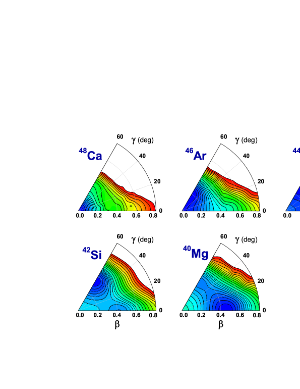
Figure 1: (Color online) Self-consistent RHB triaxial quadrupole constrained energy surfaces of $N=28$ isotones in the $\beta-\gamma$ plane ($0\leq\gamma\leq 60^{0}$). For each nucleus energies are normalized with respect to the binding energy of the global minimum. The contours join points on the surface with the same energy (in MeV).

Figure 1 displays the self-consistent RHB triaxial quadrupole constrained energy surfaces of $N=28$ isotones in the $\beta-\gamma$ plane ($0\leq\gamma\leq 60^{\circ}$), calculated using the DD-PC1 energy density functional, plus the separable pairing force Eq. (5) in the particle-particle channel. For each nucleus energies are normalized with respect to the binding energy of the absolute minimum. The contours join points on the surface with the same energy.

Starting from the spherical doubly-magic ⁴⁸Ca, we consider the even-even $N=28$ isotones obtained by successive removals of proton pairs. The binding energy maps display a rich variety of rapidly evolving shapes, and clearly demonstrate the fragility of the $N=28$ shell. By removing a pair of protons from ⁴⁸Ca, the energy surface of the corresponding isotone ⁴⁶Ar becomes soft both in $\beta$ and $\gamma$, with a shallow extended minimum along the oblate axis. Only four protons away from the doubly magic ⁴⁸Ca, DD-PC1 predicts a coexistence of prolate and oblate minima at $(\beta,\gamma)=(0.34,0^{\circ})$ and $(0.27,60^{\circ})$, respectively, in ⁴⁴S. The two minima are separated by a rather low barrier of less than 1 MeV and, therefore, one expects to find pronounced mixing of prolate and oblate configurations in the low-energy collective states of this nucleus. For ⁴²Si the binding energy displays a deep oblate minimum at $(\beta,\gamma)=(0.35,60^{\circ})$, whereas a secondary, prolate minimum is calculated $\sim 2.5$ MeV higher. Finally, with another proton pair removed, the very neutron-rich nucleus ⁴⁰Mg shows a deep prolate minimum at $(\beta,\gamma)=(0.45,0^{\circ})$.

We note that similar binding energy surfaces were also obtained in recent studies Delaroche10 ; CEA based on the self-consistent Hartree-Fock-Bogoliubov (HFB) model, using the finite-range and density-dependent Gogny D1S interaction. On the mean-field level the only qualitative difference is found for ⁴⁰Mg. For this nucleus the present calculation predicts a saddle point on the oblate axis, whereas a secondary local oblate minimum is obtained in the HFB calculation with the Gogny force.

The variation of mean-field shapes in an isotopic, or isotonic, chain is governed by the evolution of the underlying shell structure of single-nucleon orbitals. The formation of deformed minima, in particular, can be related to the occurrence of gaps or regions of low single-particle level density around the Fermi surface. In Figs. 2 – 5 we plot the neutron and proton single-particle energy levels in the canonical basis for ⁴⁶Ar, ⁴⁴S, ⁴²Si, and ⁴⁰Mg, respectively. Solid (black) curves correspond to levels with positive parity, and (red) dashed curves denote levels with negative parity. The dot-dashed (blue) curves correspond to the Fermi levels. The neutron and proton levels are plotted as functions of the deformation parameters along closed paths in the $\beta-\gamma$ plane. The panels on the left and right display prolate ($\gamma=0^{\circ}$) and oblate ($\gamma=60^{\circ}$) axially-symmetric single-particle levels, respectively. In the middle panel of each figure the neutron and proton levels are plotted as functions of $\gamma$, for a fixed value of the axial deformation $|\beta|$ at the approximate position of the mean-field minima: $|\beta|$ = 0.2 for ⁴⁶Ar, $|\beta|$ = 0.3 for ⁴⁴S, and $|\beta|$ = 0.4 for ⁴²Si and ⁴⁰Mg. In this way, starting from the spherical configuration, we follow the single-nucleon levels on a path along the prolate axis up to the approximate position of the minimum (left panel), then for this fixed value of $|\beta|$ the path from $\gamma=0^{\circ}$ to $\gamma=60^{\circ}$ (middle panel) and, finally, back to the spherical configuration along the oblate axis (right panel). Negative values of beta denote axial deformations with $\gamma=60^{\circ}$, that is, points along the oblate axis.

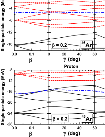
Figure 2: (Color online) Single-neutron and single-proton energy levels of ⁴⁶Ar, as functions of the deformation parameters along closed paths in the $\beta-\gamma$ plane. Solid (black) curves correspond to levels with positive parity, and (red) dashed curves denote levels with negative parity. The dot-dashed (blue) curves corresponds to the Fermi levels. The panels on the left and right display prolate ($\gamma=0^{\circ}$) and oblate ($\gamma=60^{\circ}$) axially-symmetric single-particle levels, respectively. In the middle panel of each figure the neutron and proton levels are plotted as functions of $\gamma$, for a fixed value of the axial deformation $|\beta|$ at the approximate position of the mean-field minimum.

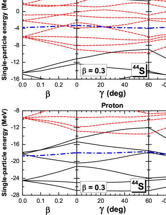
Figure 3: (Color online) Same as described in the caption to Fig. 2 but for the nucleus ⁴⁴S.

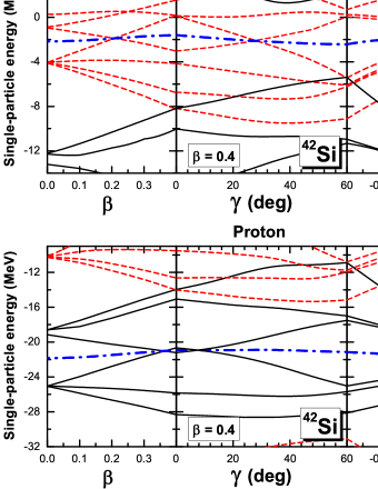
Figure 4: (Color online) Same as described in the caption to Fig. 2 but for the nucleus ⁴²Si.

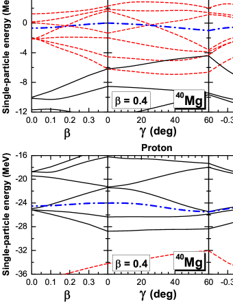
Figure 5: (Color online) Same as described in the caption to Fig. 2 but for the nucleus ⁴⁰Mg.

Figures 2 – 5 elucidate the principal characteristics of structural changes in neutron-rich $N=28$ nuclei: the near degeneracy of the $d_{3/2}$ and $s_{1/2}$ proton orbitals, and the reduction of the size of the $N=28$ shell gap OSor.10 . Between the doubly magic ⁴⁸Ca and ⁴⁶Ar the spherical gap $N=28$ decreases from 4.73 MeV to 4.48 MeV (cf. Table 1), in excellent agreement with data: from 4.80 MeV in ⁴⁸Ca to 4.47 MeV in ⁴⁶Ar Gaudefroy06 ; Gaudefroy07 . Nevertheless, the gap between occupied and unoccupied neutron levels in ⁴⁶Ar is still largest at the spherical configuration, as shown in the upper panel of Fig. 2. We note, in particular, the agreement of the calculated energies of spherical neutron states with experimental single-neutron energies Gaudefroy06 . For the proton states shown in the lower panel, the largest gap is found at $|\beta|$ = 0.2 and $\gamma=60^{\circ}$, that is, on the oblate axis. The competition between the spherical configuration favored by neutron states and the oblate shape favored by proton states, leads to the shallow extended oblate minimum shown in Fig. 1. Two protons less, and the spherical $N=28$ gap is reduced by another 620 keV to 3.86 MeV in ⁴⁴S. The largest gap between neutron states is not the spherical one like in ⁴⁶Ar, however, but at the oblate deformation $|\beta|\approx$ 0.3 and $\gamma=60^{\circ}$ (upper panel of Fig. 3). The removal of two protons lowers the energy of the corresponding Fermi level, and for ⁴⁴S the largest gap is found on the prolate axis (lower panel of Fig. 3). The formation of the oblate neutron and prolate proton gaps is at the origin of the coexistence of deformed shapes in ⁴⁴S (cf. Fig. 1). In ⁴²Si both neutron and proton gaps are on the oblate axis resulting in the pronounced oblate minimum at $|\beta|\approx$ 0.35. Finally, the deep prolate minimum at $\beta\approx$ 0.35 in ⁴⁰Mg arises because of the neutron gap and, especially pronounced, proton gap on the prolate axis. We note that the largest neutron gap for this nucleus is still on the oblate side but, because the protons strongly favor the prolate configuration, it produces only a saddle point on the oblate axis, as shown in Fig. 1.

Table 1: The DD-PC1 RHB theoretical neutron $N=28$ spherical energy gaps, and the corresponding values of the axial deformation for the minima of the quadrupole binding energy maps of ⁴⁸Ca, ⁴⁶Ar, ⁴⁴S, ⁴²Si, and ⁴⁰Mg. Negative values of $\beta$ denote oblate shapes.

	$\Delta^{\rm sph.}_{N=28}$	$\beta_{\rm min}$
48Ca	4.73	0.00
46Ar	4.48	-0.19
44S	3.86	0.34
42Si	3.13	-0.35
40Mg	2.03	0.45

The erosion of the spherical $N=28$ shell is also shown in Table 1, where we include the DD-PC1 RHB theoretical neutron $N=28$ spherical energy gaps, and the corresponding values of the axial deformation for the minima of the quadrupole binding energy maps of ⁴⁸Ca, ⁴⁶Ar, ⁴⁴S, ⁴²Si, and ⁴⁰Mg. Both experiment and theory point toward a strong reduction of the $N=28$ gap as more protons are removed and, thus, the isotones become more neutron-rich. N=28 is the first “magic” number produced by the spin-orbit part of the single-nucleon potential and, therefore, a relativistic mean-field model automatically reproduces the N=28 gap because it naturally includes the spin-orbit interaction and the correct isospin dependence of this term, as it was already shown in the axial RHB calculation of neutron-rich N=28 nuclei Lalazissis99 . Experimentally, indirect evidence of the erosion of the gap has been obtained by following the evolution of excitation energies of the $2^{+}_{1}$ state and the E2 transitions in $N=28$ isotones and neighboring nuclei Sorlin93 ; Scheit96 ; Glasmacher97 ; Gaudefroy06 ; Force10 . The experimental results can be reproduced by both mean-field Lalazissis99 ; Peru00 and shell model Nowacki09 calculations. As shown in Table 1, the DD-PC1 RHB calculation predicts a reduction of the spherical $N=28$ shell gap from 4.73 MeV in the doubly-magic nucleus ⁴⁸Ca to 2.03 MeV in the well-deformed ⁴⁰Mg. We note that the theoretical values of the spherical shell gap for ⁴⁸Ca and ⁴⁶Ar are very close to data: 4.80 MeV in ⁴⁹Ca, and 4.47 MeV in ⁴⁷Ar, obtained by neutron stripping reactions Gaudefroy06 ; Gaudefroy07 .

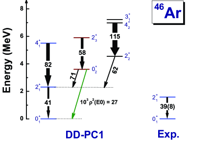
Figure 6: (Color online) The spectrum of ⁴⁶Ar calculated with the DD-PC1 relativistic density functional (left), compared to data NNDC (right) for the excitation energy of $2^{+}_{1}$, and the reduced electric quadrupole transition B(E2) (in units of $e^{2}{\rm fm}^{4}$). The prediction for the electric monopole transition strength $\rho^{2}(E0;0^{+}_{2}\rightarrow 0^{+}_{1})$ is also included in the theoretical spectrum.

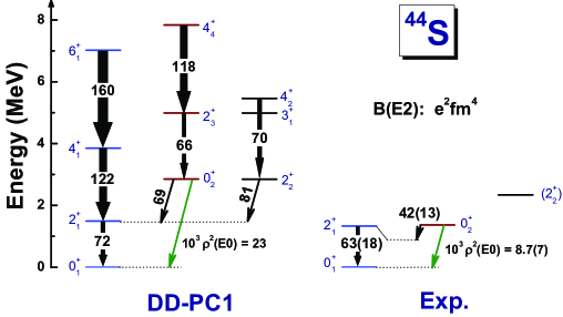
Figure 7: (Color online) Same as described in the caption to Fig. 6 but for the nucleus ⁴⁴S. The data are from Refs. Glasmacher97 ; Force10 .

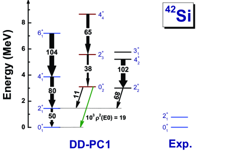
Figure 8: (Color online) Same as described in the caption to Fig. 6 but for the nucleus ⁴²Si. The data are from Ref. Bastin07 .

III.2 Low-energy collective spectra

Starting from constrained self-consistent solutions of the RHB equations, that is, using single-quasiparticle energies and wave functions that correspond to each point on the energy surfaces shown in Fig. 1, the parameters that determine the collective Hamiltonian: the mass parameters $B_{\beta\beta}$, $B_{\beta\gamma}$, $B_{\gamma\gamma}$, three moments of inertia $\mathcal{I}_{k}$, as well as the zero-point energy corrections, are calculated as functions of the quadrupole deformations $\beta$ and $\gamma$. The diagonalization of the resulting Hamiltonian yields the excitation energies and reduced transition probabilities. In Figs. 6 – 8 we display the spectra of ⁴⁶Ar, ⁴⁴S, and ⁴²Si calculated with the DD-PC1 relativistic density functional plus the separable pairing force Eq. (5), in comparison to available data for the excitation energies, reduced electric quadrupole transition probabilities B(E2) (in units of $e^{2}{\rm fm}^{4}$), and the electric monopole transition strength $\rho^{2}(E0;0^{+}_{2}\rightarrow 0^{+}_{1})$. We emphasize that this calculation is completely parameter-free, that is, by using the self-consistent solutions of the RHB single-nucleon equations, physical observables, such as transition probabilities and spectroscopic quadrupole moments, are calculated in the full configuration space and there is no need for effective charges. Using the bare value of the proton charge in the electric quadrupole operator, the transition probabilities between eigenstates of the collective Hamiltonian can directly be compared to data.

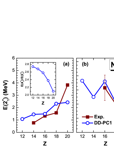
Figure 9: (Color online) Evolution of the characteristic observables $E(2^{+}_{1})$ and $B(E2;2^{+}_{1}\rightarrow 0^{+}_{1})$ (in ${\rm e}^{2}{\rm fm}^{4}$) with proton number in $N=28$ isotones. The ratio between the excitation energies of the first $4^{+}$ and $2^{+}$ states is also displayed in the inset. The microscopic values calculated with the energy density functional DD-PC1 are shown in comparison with available data.

Before considering the excitation spectra of individual nuclei and, in particular, shape coexistence in ⁴⁴S, in Fig. 9 we illustrate the evolution with proton number of characteristic collective observables: the excitation energy of the first $2^{+}$ state, the ratio $E(4^{+}_{1})/E(2^{+}_{1})$, and the reduced transition probability B(E2; $2^{+}_{1}\to 0^{+}_{1}$). The rapid decrease of the ratio $E(4^{+}_{1})/E(2^{+}_{1})$ from $\approx 2.8$ in ⁴⁰Mg to $\approx 2.1$ in ⁴⁸Ca is characteristic for a transition from a deformed rotational nucleus to a spherical vibrator. Note, however, that even in the case of ⁴⁰Mg the value of $E(4^{+}_{1})/E(2^{+}_{1})$ is considerably below the rigid-rotor limit of 3.3. The excitation energy of the first excited state $2^{+}_{1}$ can directly be compared to data. The calculated $E(2^{+}_{1})$ increases with proton number toward the doubly magic ⁴⁸Ca, but the predicted rise in energy is not as sharp as in experiment. In fact, one expects that in deformed nuclei, e.g ⁴²Si, the calculated $E(2^{+}_{1})$ is above the experimental excitation energy, because of the well-known fact that the Inglis-Belyaev formula Eq. (13) predicts effective moments of inertia that are smaller than empirical values. The moments of inertia can generally be improved by including the Thouless-Valatin (TV) dynamical rearrangement contributions Delaroche10 , but the calculation of the TV moments of inertia Thouless62 has not yet been implemented in the collective Hamiltonian used in the present calculation. The panel on the right of Fig. 9 displays the evolution with proton number of another characteristic collective observable: $B(E2;2^{+}_{1}\to 0^{+}_{1})$ (in $e^{2}{\rm fm}^{4}$). The calculation reproduces the empirical decrease of $B(E2;2^{+}_{1}\to 0^{+}_{1})$ with proton number and, in particular, we notice the excellent agreement between the parameter-free theoretical predictions and data for ⁴⁴S and ⁴⁶Ar.

Figure 6 displays the low-energy spectrum of ⁴⁶Ar. The excitation energy $E(2^{+}_{1})$ is calculated considerably above the experimental state, whereas the $B(E2;2^{+}_{1}\to 0^{+}_{1})$ reproduces the experimental value. In the present analysis we particularly focus on ⁴⁴S, for which data that indicate shape coexistence were reported recently Force10 . Already the data on the low energy of the first $2^{+}$ state and the enhanced $B(E2;2^{+}_{1}\to 0^{+}_{1})$ of 63(18) $e^{2}{\rm fm}^{4}$ Glasmacher97 pointed towards a possible deformation of the ground state of ⁴⁴S. More recently, the structure of this nucleus was studied by using delayed $\gamma$ and electron spectroscopy, and new data were reported for the reduced transition probability $B(E2;2^{+}_{1}\to 0^{+}_{2})=8.4(26)$ $e^{2}{\rm fm}^{4}$, and the monopole strength $\rho^{2}(E0;0^{+}_{2}\to 0^{+}_{1})=8.7(7)\times 10^{-3}$ Force10 . From a comparison to shell model calculations, a prolate-spherical shape coexistence was inferred, and a two-level mixing model was used to extract a weak mixing between the two configurations. The spectrum of ⁴⁴S calculated in this work is compared to available data in Fig. 7. The model nicely reproduces both the excitation energy and the reduced transition probability $B(E2;2^{+}_{1}\to 0^{+}_{1})$ for the first excited state $2^{+}_{1}$, and the theoretical value for $B(E2;0^{+}_{2}\to 2^{+}_{1})$ is also in good agreement with data. The experimental ratio $B(E2;2^{+}_{1}\to 0^{+}_{1})/B(E2;2^{+}_{1}\to 0^{+}_{2})$ is 7.5, and the calculated value is 5.2. The excitation energy of the state $0^{+}_{2}$, however, is calculated much higher than the experimental counterpart. Together with the fact that the calculated monopole transition strength $\rho^{2}(E0;0^{+}_{2}\rightarrow 0^{+}_{1})(\times 10^{3})$ = 23 is larger than the corresponding experimental value of 8.7(7), this result indicates that there is more mixing between the theoretical states $0^{+}_{1}$ and $0^{+}_{2}$ than what can be inferred from the data.

The low-lying $0^{+}_{2}$ state with the excitation energy $1.365$ MeV, the rather weak interband transition probability B(E2; $2^{+}_{1}\to 0^{+}_{2}$)=8.4(26) $e^{2}{\rm fm}^{4}$, and the monopole strength $\rho^{2}(E0;0^{+}_{2}\to 0^{+}_{1})=8.7(7)\times 10^{-3}$ have been regarded as fingerprints of shape coexistence in ⁴⁴S Force10 . One reason for the more pronounced mixing between the calculated $0^{+}_{1}$ and $0^{+}_{2}$ in this work and, consequently, the higher excitation energy of $0^{+}_{2}$, could be the particular choice of the energy density functional and/or the treatment of pairing correlations Li11 . The predicted barrier between the prolate and oblate minima (cf. Fig. 1) could, in fact, be too low. Another reason for the high excitation energy of $0^{+}_{2}$ could be the approximation used in the calculation of mass parameters (vibrational inertial functions). In the current version of the model the mass parameters are determined by using the cranking approximation Eqs. (14) and (15), in which the time-odd components (the so-called Thouless-Valatin dynamical rearrangement contributions) are omitted. Recently an efficient microscopic derivation of the five-dimensional quadrupole collective Hamiltonian has been developed, based on the adiabatic self-consistent collective coordinate method Hinohara10 . In this model the moments of inertia and mass parameters are determined from local normal modes built on constrained Hartree-Fock-Bogoliubov states, and the TV dynamical rearrangement contributions are treated self-consistently. For the illustrative case of ⁶⁸Se, it has been shown that the self-consistent inclusion of the time-odd components of the mean-field can lead to an increase of the mass parameters by $30\%\sim 200\%$, depending on the deformation. In fact, in the present calculation an enhancement of the cranking masses by a factor $\sim 2$ brings the calculated excitation energies, and also the monopole strength $\rho^{2}(E0;0^{+}_{2}\to 0^{+}_{1})$, in very close agreement with the experimental spectrum.

In Table 2 we compare the experimental excitation energies of the states $2^{+}_{1}$, $0^{+}_{2}$, and $2^{+}_{2}$, the reduced transition probabilities $B(E2;2^{+}_{1}\rightarrow 0^{+}_{1})$ ($e^{2}{\rm fm}^{4}$), $B(E2;2^{+}_{1}\rightarrow 0^{+}_{2})$, and the monopole strength $\rho^{2}(E0;0^{+}_{2}\to 0^{+}_{1})\times 10^{3}$ in ⁴⁴S, to the results of the present work, the five-dimensional GCM(GOA) calculation with the Gogny D1S interaction CEA , the angular-momentum projected GCM calculation restricted to axial shapes (AMP GCM) with the Gogny D1S interaction Guzman02 , and to shell-model calculations Force10 . One might notice that all three models based on constrained self-consistent mean-field calculations of the binding energy maps (curves in the case of axially-symmetric AMP GCM), reproduce the data with similar accuracy. It is interesting that only the axially-symmetric calculation reproduces the very low excitation energy of the state $0^{+}_{2}$, whereas the result of the five-dimensional GCM(GOA) calculation, although it was also based on the Gogny D1S interaction, is even above the energy obtained with DD-PC1. Table 2 shows that the best overall agreement with data is obtained in the shell-model (SM) calculation of Ref. Force10 , using the effective interaction SDPF-U Nowacki09 for $0\hbar\omega$ SM calculations in the $sd-pf$ valence space, and with a particular choice of the proton and neutron effective charges.

Table 2: Excitation energies (in MeV) of the states $2^{+}_{1}$, $0^{+}_{2}$, and $2^{+}_{2}$, $B(E2;2^{+}_{1}\rightarrow 0^{+}_{1})$ ($e^{2}{\rm fm}^{4}$), $B(E2;2^{+}_{1}\rightarrow 0^{+}_{2})$, and the monopole strength $\rho^{2}(E0;0^{+}_{2}\to 0^{+}_{1})\times 10^{3}$ in ⁴⁴S. The experimental values Sohler02 ; Force10 are compared to the results of the present work, the five-dimensional GCM(GOA) calculation with the Gogny D1S interaction CEA , the angular-momentum projected GCM calculation restricted to axial shapes (AMPGCM) with the Gogny D1S interaction Guzman02 , and to shell-model calculations Force10 .

	Experiment	This work	GCM(GOA) CEA	AMPGCM Guzman02	Shell Model Force10
$E(2^{+}_{1})$	1.329(1)	1.491	1.267	1.410	1.172
$E(0^{+}_{2})$	1.365(1)	2.852	3.611	1.070	1.137
$E(2^{+}_{2})$	2.335(39)	2.851	2.557	1.830	2.140
$B(E2;2^{+}_{1}\rightarrow 0^{+}_{1})$	63(18)	72	105	75	75
$B(E2;2^{+}_{1}\rightarrow 0^{+}_{2})$	8.4(2.6)	14	6.3	-	19
$\rho^{2}(E0;0^{+}_{2}\to 0^{+}_{1})(\times 10^{3})$	8.7(7)	23	5.4	-	-

Based on the data included in Table 2 and on the SM calculation with the SDPF-U effective interaction, in Ref. Force10 it was deduced that ⁴⁴S exhibits a shape coexistence between a prolate ground state ($\beta\approx 0.25)$ and a rather spherical $0^{+}_{2}$ state. The sequence of ground-state band states $0^{+}_{1}$, $2^{+}_{1}$, $4^{+}_{2}$, and $6^{+}_{2}$, is connected by strong E2 transitions, and the excited states are characterized by the intrinsic quadrupole moment $Q_{0}\approx 60$ $e~{}{\rm fm}^{2}$. This sequence was interpreted as a rotational band of an axially deformed prolate shape with $\beta\approx 0.25$. The calculated $2^{+}_{2}$ state has a smaller quadrupole moment $Q_{0}=-0.3$ $e~{}{\rm fm}^{2}$, compatible with a spherical shape, and is connected by a strong E2 transition to the $0^{+}_{2}$ state. These SM results, therefore, indicate a prolate-spherical shape coexistence in ⁴⁴S Force10 .

To analyze configuration mixing in the low-energy spectrum based on the functional DD-PC1, in Fig. 10 we plot the probability density distributions for the three lowest states of the ground-state band: $0^{+}_{1}$, $2^{+}_{1}$, and $4^{+}_{1}$, the state $0^{+}_{2}$, and the two states $2^{+}_{2}$ and $2^{+}_{3}$. For a given collective state Eq. (16), the probability density distribution in the $(\beta,\gamma)$ plane is defined by:

$$\rho_{I\alpha}(\beta,\gamma)=\sum\limits_{K\in\Delta I}|\psi^{I}_{\alpha K}(\beta,\gamma)|^{2}\beta^{3},$$ (20)

with the normalization:

$$\int^{\infty}_{0}\beta{\rm d}\beta\int^{2\pi}_{0}\rho_{I\alpha}(\beta,\gamma)\ |\sin 3\gamma|~{}{\rm d}\gamma=1.$$ (21)

The probability distribution of the ground state $0^{+}_{1}$ indicates a deformation $|\beta|\geq 0.3$, extended in the $\gamma$ direction from the prolate configuration at $\gamma=0$ to the oblate configuration at $\gamma=60^{\circ}$. The average deformation is $(\langle\beta\rangle,\langle\gamma\rangle)=(0.32,26^{\circ})$, and the $\gamma$-softness reflects the ground-state mixing of configurations based on the prolate and oblate minima of the potential (cf. Fig. 1). With the increase of angular momentum in the ground-state band, e.g. $2^{+}_{1}$, $4^{+}_{1}$, etc., the states are progressively concentrated on the prolate axis. For instance, $(\langle\beta\rangle,\langle\gamma\rangle)=(0.35,23^{\circ})$ for $2^{+}_{1}$. The average $\beta$-deformation in the ground-state band gradually increases because of centrifugal stretching. Again we note that the empirical value $B(E2;2^{+}_{1}\rightarrow 0^{+}_{2})$ is accurately reproduced by the present calculation using just the bare proton charge. In contrast to the SM prediction Force10 , the state $0^{+}_{2}$ is predominantly prolate, although one notices a relatively large overlap between the wave functions of the states $0^{+}_{1}$ and $0^{+}_{2}$. The mixing between these states is probably one of the reasons for the high excitation energy of the second $0^{+}$ state, as predicted by the present calculation (cf. Fig. 7). The probability distribution of the state $2^{+}_{3}$ is concentrated on the prolate axis, and this state is connected by a strong transition to $0^{+}_{2}$: $B(E2;2^{+}_{3}\to 0^{+}_{2})=66$ $e^{2}{\rm fm}^{4}$, comparable to $B(E2;2^{+}_{1}\to 0^{+}_{1})$. We note, however, that for the ”coexisting” band based on $0^{+}_{2}$ the calculated ratio $E(4^{+})/E(2^{+})$ is only 2.33.

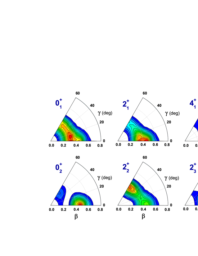
Figure 10: (Color online) Probability distribution Eq. (20) in the $\beta-\gamma$ plane for the lowest collective states of ⁴⁴S, predicted by DD-PC1 energy density functional.

The calculated second $2^{+}$ state displays a probability distribution extended in the $\gamma$-direction and peaked on the oblate axis. As shown in Fig. 7 and Table 2, this state is very close to the experimental candidate for the $2^{+}_{2}$ state, which was suggested to be at 2335(39) keV by placing the 988 keV transition Sohler02 on top of the $0^{+}_{2}$ or $2^{+}_{1}$ state Force10 . The theoretical $2^{+}_{2}$ state can be interpreted as the (quasi)-$\gamma$ band-head according to the strong E2 transitions to the states $3^{+}_{1}$ and $4^{+}_{2}$. For the three lowest $2^{+}$ states, in Table 3 we include the percentage of the $K=0$ and $K=2$ components in the corresponding collective wave functions Eq. (16) (K denotes the projection of the angular momentum on the intrinsic 3-axis), as well as the spectroscopic quadrupole moments. The wave functions of the states $2^{+}_{1}$ and $2^{+}_{3}$ are dominated by $K=0$ components, and the spectroscopic quadrupole moments are negative (prolate configurations) with comparable magnitudes. The positive quadrupole moment of $2^{+}_{2}$ points to a predominant oblate configuration, and the $\approx 80\%$ contribution of the $K=2$ component in the wave function confirms that this state is the band-head of a (quasi) $\gamma$-band (note the formation of the doublet $3^{+}_{1}$ and $4^{+}_{2}$).

Table 3: Percentage of the $K=0$ and $K=2$ components (projection of the angular momentum on the body-fixed symmetry axis) for the collective wave functions of the three lowest $2^{+}$ states in ⁴⁴S, and the corresponding spectroscopic quadrupole moments (in $e~{}{\rm fm}^{2}$).

	$K=0$	$K=2$	$Q_{\rm spec.}$
$2^{+}_{1}$	88.4	11.6	-10.9
$2^{+}_{2}$	21.5	78.5	7.8
$2^{+}_{3}$	80.0	20.0	-9.6

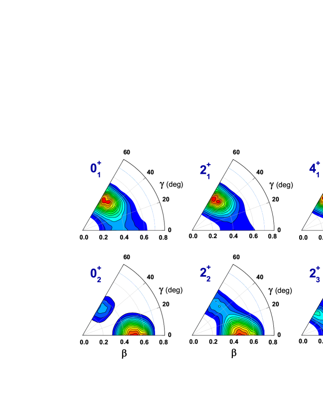
Figure 11: (Color online) Same as described in the caption to Fig. 10 but for the nucleus ⁴²Si.

Finally, Fig. 8 shows the low-energy collective spectrum of ⁴²Si. Even though the excitation spectrum and transition pattern appear to be similar to that of ⁴⁴S, with the exception of a considerably weaker E2 transition $0^{+}_{2}\to 2^{+}_{1}$ (cf. Fig. 7), the ground-state band of this nucleus is in fact based on the oblate minimum shown in the binding energy map of Fig. 1. This is nicely illustrated in Fig. 11 where, just like in the case of ⁴⁴S in Fig. 10, we plot the probability distributions of the collective wave functions $0^{+}_{1}$, $2^{+}_{1}$, and $4^{+}_{1}$, the state $0^{+}_{2}$, and the two states $2^{+}_{2}$ and $2^{+}_{3}$. The wave functions of the yrast states $0^{+}_{1}$, $2^{+}_{1}$, and $4^{+}_{1}$ are concentrated along the oblate axis. The state $0^{+}_{2}$ is strongly prolate deformed, with a peak in the probability distribution at $\beta\approx 0.5$. This state has a much smaller overlap with $2^{+}_{1}$ than in the case of ⁴⁴S, and this explains the correspondingly weaker transition. For ⁴²Si, therefore, the solution of the collective Hamiltonian based on the DD-PC1 functional, predicts a coexistence of the oblate yrast band and the prolate sequence built on the strongly deformed state $0^{+}_{2}$. As already shown in Fig. 9, the present calculation does not reproduce the exceptionally low excitation energy of the state $2^{+}_{1}$: 770(19) keV Bastin07 . It is interesting, however, that the calculated excitation energy of this state is very close to the SM prediction obtained using the SDPF-NR effective interaction Bastin07 . Only by removing from the SDPF-NR a schematic pairing Hamiltonian in the $pf$ shell, that is, by using the new effective interaction SDPF-U Nowacki09 , the $2^{+}$ excitation energies of the silicon isotopes can be brought in agreement with experiment.

IV Summary

Structure phenomena related to the evolution of single-nucleon levels and shells in neutron-rich nuclei present a very active area of experimental and theoretical research. Among the microscopic models that can be used for a theoretical analysis of these phenomena, the framework of nuclear energy density functionals (EDFs) presently provides a complete and accurate description of ground-state properties and collective excitations across the entire chart of nuclides. In this work we have used the recently introduced relativistic EDF DD-PC1 NVR.08 to study the erosion of the $N=28$ spherical shell in neutron-rich nuclei and the related phenomenon of shape evolution and shape coexistence in the $N=28$ isotones ⁴⁶Ar, ⁴⁴S, ⁴²Si, and ⁴⁰Mg. Pairing correlations have been taken into account by employing an interaction that is separable in momentum space, and is completely determined by two parameters adjusted to reproduce the empirical bell-shaped pairing gap in symmetric nuclear matter Niksic10 .

The N=28 shell closure is the first neutron magic number produced by the spin-orbit part of the single-nucleon potential and, therefore, a relativistic mean-field model automatically reproduces the N=28 spherical gap because it naturally includes the spin-orbit interaction and the correct isospin dependence of this term, as it was shown more than ten years ago in the axial RHB calculation of neutron-rich N=28 nuclei Lalazissis99 . In particular, in the RMF approach there is no need for a tensor interaction to reproduce the isospin dependence (quenching) of the spherical N=28 gap in neutron-rich nuclei, as also shown in the present work in Table 1, compared to available data.

The functional DD-PC1 was adjusted exclusively to the experimental masses of a set of 64 deformed nuclei in the mass regions $A\approx 150-180$ and $A\approx 230-250$. The present study of the $N=28$ isotones thus presents an extrapolation of DD-PC1 to a completely different region of the nuclide chart, and a further test of the universality of nuclear EDFs. It is not at all obvious that such an extrapolation will produce results in agreement with experiment, especially in a detailed comparison with spectroscopic data. The fact that it does is remarkable, and justifies the approach to nuclear structure based on universal energy density functionals.

Starting from self-consistent binding energy maps in the $\beta-\gamma$ plane, calculated in the relativistic Hartree-Bogoliubov (RHB) model based on the functional DD-PC1, a recent implementation of the collective Hamiltonian for quadrupole vibrations and rotations has been used to calculate the excitation spectra and transition rates of ⁴⁶Ar, ⁴⁴S, ⁴²Si, and ⁴⁰Mg. The parameters that determine the collective Hamiltonian: the vibrational inertial functions, the moments of inertia, and the zero-point energy corrections, are calculated using the single-quasiparticle energy and wave functions that correspond to each point on the self-consistent RHB binding energy surface of a given nucleus. The diagonalization of the collective Hamiltonian yields the excitation energies and wave functions used to calculate various observables.

The calculation performed in this work has shown that the relativistic functional DD-PC1 provides an accurate microscopic interpretation of the strong reduction of the $N=28$ spherical energy gap in neutron-rich nuclei, and a quantitative description of the evolution of shapes in $N=28$ isotones in terms of single-nucleon orbitals as functions of the quadrupole deformation parameters $\beta$ and $\gamma$. In particular, the predicted values for the spherical shell gap in ⁴⁸Ca (4.73 MeV) and in ⁴⁶Ar (4.48 MeV), are very close to the data: 4.80 MeV in ⁴⁹Ca and 4.47 MeV in ⁴⁷Ar. The solutions of the collective Hamiltonian based on DD-PC1 reproduce the evolution with proton number of characteristic collective observables the excitation energy of the first $2^{+}$ state, the ratio $E(4^{+}_{1})/E(2^{+}_{1})$, and the reduced transition probability B(E2; $2^{+}_{1}\to 0^{+}_{1}$). In the present work we have focused on ⁴⁴S, for which recent data point towards a coexistence of shapes with different deformations in the low-energy excitation spectrum. It has been shown that the formation of the oblate neutron and prolate proton gaps, illustrated in Fig. 3, is at the origin of the predicted coexistence of deformed shapes in ⁴⁴S. The spectroscopic results have been compared to available data, to triaxial (collective Hamiltonian) and axial (generator coordinate method) calculations based on the Gogny D1S HFB self-consistent mean-field energy maps, and to recent shell-model (SM) calculations using the new SDPF-U effective interaction. The present results are in qualitative agreement with previous calculations based on the Gogny D1S HFB model and, in particular, reproduce the data on both the excitation energy of the first excited state $2^{+}_{1}$ and the reduced transition probability $B(E2;2^{+}_{1}\to 0^{+}_{1})$, and the theoretical value for $B(E2;0^{+}_{2}\to 2^{+}_{1})$ is also in good agreement with data. The experimental ratio $B(E2;2^{+}_{1}\to 0^{+}_{1})/B(E2;2^{+}_{1}\to 0^{+}_{2})$ is 7.5, and the calculated value is 5.2. The theoretical monopole transition strength $\rho^{2}(E0;0^{+}_{2}\rightarrow 0^{+}_{1})(\times 10^{3})$ = 23 is somewhat larger than the corresponding experimental value of 8.7(7). The calculation of transition rates in the collective Hamiltonian model is completely parameter-free. One might notice that the results predicted by the functional DD-PC1 have been compared to those obtained using effective interactions that were fine-tuned to data that include also this mass region, or adjusted exclusively to data in this region of the mass table (shell-model interactions). The fact that a global density functional can even compete in a spectroscopic calculation with shell-model interactions specifically customized to this mass region, and the level of agreement with experiment, presents a valuable result.

A discrepancy with respect to experiment in ⁴⁴S is the high excitation energy predicted for the state $0^{+}_{2}$, a factor of two compared to data. It appears that the model predicts too much mixing between the two lowest $0^{+}$ states, and this leads to an enhancement of the corresponding monopole transition strength. The pronounced mixing between the calculated $0^{+}_{1}$ and $0^{+}_{2}$ states, and the resulting repulsion, could be at the origin of the high excitation energy of $0^{+}_{2}$. The most obvious reason is that this is an intrinsic prediction of the functional DD-PC1. To check this one would have to perform calculations using different functionals Zhao10 . However, since also the Gogny D1S + 5DCH model yields a similar result, the functional itself probably is not the main problem. A more probable reason is that the mass parameters calculated in the cranking approximation are simply too small, as discussed in Sec. III.2. Finally, the excited $0^{+}$ state could also have pronounced non-collective components that are not included in our model space (2-quasiparticle contributions). This is certainly a possibility, and it would partially explain why the calculated B(E2) to the first $2^{+}$ state is larger than the experimental value. The shell-model calculation of Ref. Force10 predicts the excitation energy of $0^{+}_{2}$ in better agreement with experiment, but the calculated B(E2) for the transition from the first $2^{+}$ state is more than a factor two larger than the experimental value (only about 50% larger in the present calculation). Therefore, it appears that the structure of the second $0^{+}$ state in ⁴⁴S remains an open problem.

This present analysis of low-energy spectra of $N=28$ isotones has clearly demonstrated the advantages of using EDFs in the description of deformed nuclei: an intuitive mean-field interpretation in terms of coexisting intrinsic shapes and the evolution of single-particle states, spectroscopic calculations performed in the full model space of occupied states, and the universality of EDFs that enables their applications to nuclei in different mass regions, including short-lived systems far from stability.