Besides the familiar D-branes, string theory contains a vast number of other non-perturbative objects. While a complete classification is lacking, many of these objects are related to each other through various dualities. Codimension two objects play a special role, because their charges are no longer additive but are instead expressed in terms of holonomies of scalar fields, which is given by an element of the relevant duality group. In this paper we present a detailed exposition of these “exotic” objects, the charges they carry, and their connection to non-geometric compactifications. Despite the name “exotic branes,” these objects are in fact ubiquitous in string theory, as they can automatically appear when describing bound states of conventional branes, and as such may be of particular importance in describing the microscopic degrees of freedom of black holes.

1 Introduction

String theory includes various extended objects as collective excitations, such as D-branes. The $U$-duality symmetry [1] which maps these objects into one another has played a pivotal role in the development of string theory and provided crucial insights into its non-perturbative behavior. When string/M-theory is compactified to lower dimensions, the $U$-duality group gets enhanced, relating objects that were not related in higher dimensions. For example, when M-theory is compactified on $T^{k}$, the lower $(d=11-k)$ dimensional theory has an $E_{k(k)}({\mathbb{R}})$ symmetry as the $U$-duality group, at the level of classical supergravity. This continuous $E_{k(k)}({\mathbb{R}})$ symmetry is believed to be broken to a discrete $E_{k(k)}({\mathbb{Z}})$ symmetry in the quantum theory [1].

As the torus dimension $k$ increases, the number of gauge fields in the lower ($d=11-k$) dimensional theory increases, and so does that of associated charged particles. The spectrum of these charged particles represent the orbit of the $U$-duality group. For $d\geq 4$, the 11-dimensional origin of such charged particles is easily understood; they are ordinary branes partially wrapped on $T^{k}$. For $d\leq 3$, however, the lower dimensional theories contain particles, called exotic states, whose higher-dimensional origin is less obvious [2, 3, 4, 5, 6]. In Type II language, most of them have tension proportional to $g_{s}^{-3}$ or $g_{s}^{-4}$, clearly indicating that they cannot be explained in terms of ordinary branes whose tension can at most be $\sim g_{s}^{-2}$.

For example, in Type II superstring compactified on $T^{2}$, consider an NS5-brane extending along six of the eight remaining non-compact directions, not wrapping the internal $T^{2}$ (Table 1).

	1	2	3	4	5	6	7	8	9
NS5	$\cdot$	$\cdot$	$\bigcirc$	$\bigcirc$	$\bigcirc$	$\bigcirc$	$\bigcirc$	$\cdot$	$\cdot$
$\downarrow T_{89}\rule{0.0pt}{12.91663pt}$
$5^{2}_{2}$	$\cdot$	$\cdot$	$\bigcirc$	$\bigcirc$	$\bigcirc$	$\bigcirc$	$\bigcirc$	$\circledcirc$	$\circledcirc$

Table 1: Two transverse $T$-duality transformations on an NS5-brane produce an exotic $5^{2}_{2}$-brane. “$\,\cdot\,$” (“$\,\bigcirc\,$”) indicates that the brane is localized (extended) in that direction. The mass of the $5^{2}_{2}$ is proportional to the squared radii of the directions with “$\,\circledcirc\,$”.

It is well-known that, if we perform a $T$-duality along one of the $T^{2}$ directions, we obtain a Kaluza–Klein (KK) monopole. However, it is much less known that, if we $T$-dualize further along the remaining direction of the $T^{2}$, we obtain a codimension-2 exotic state called $5^{2}_{2}$; see Table 1. As was noted in [7] and will be reviewed later, the $5^{2}_{2}$ solution is a non-geometric background known as a $T$-fold [10]; namely, as we go around it, the internal $T^{2}$ is non-trivially fibered and does not come back to itself, but rather to a $T$-dual version. Other exotic states can be obtained by further application of $U$-duality transformations on this $5^{2}_{2}$. They have non-trivial $U$-duality monodromies around them, i.e., the spacetime is glued together around them by $U$-duality twists, and they are hence non-geometric $U$-folds [10]. These exotic states can be thought of as codimension-2 branes and we will call them exotic branes.

Being dual to the standard branes such as D-branes, exotic branes are as essential ingredients of string theory as standard branes are, and are worth studying on its own. In particular, the fact that their charge is characterized by the non-trivial monodromy around them is a novel and peculiar feature and is expected to lead to interesting structures; this was indeed the case with F-theory 7-branes, of which exotic branes can be thought of as generalizations. For example, the monodromic structure of F-theory 7-branes were crucial for realizing gauge theories with exceptional gauge groups [11, 12, 13, 14, 15, 16]. Furthermore, the non-geometric nature of the monodromy is of much interest in view of the recent developments in the double field theory [17, 18, 19] (for reviews, see [20, 21]) and generalizations thereof [22, 23, 24, 25, 26], which is a framework to incorporate stringy non-geometric nature of spacetime.

One might think that such codimension-2 objects are problematic due to logarithmic divergences [27]; generally, codimension-2 objects will backreact on the spacetime very badly and destroy the asymptotics. Also, exotic branes were found in three dimensions whereas our universe is four dimensional. Based on these, one might conclude that exotic branes are irrelevant as long as we are concerned with physics of ordinary branes in realistic spacetimes. However, these are naive and incorrect because of the supertube effect [28]—the spontaneous polarization phenomenon that occurs when we bring a particular combination of charges together. Let us briefly recall what this phenomenon is. A basic example of the supertube effect is

$$\rm D0+F1(1)\to d2(1\psi)+p(\psi),$$ (1.1)

in which D0-branes and fundamental strings along $x^{1}$ spontaneously polarize into a D2-brane extending along $x^{1}$ and an arbitrary closed curve in the transverse eight directions parametrized by $\psi$. On the D2-brane worldvolume, there is also a density of momentum charge along $\psi$. Note that the D2 charge did not exist in the original configuration. However, this does not violate charge conservation, because the D2 is along a closed curve and there is no net D2 charge but only a D2 dipole charge. We wrote the lowercase “d2” on the right hand side of (1.1) to clarify that the D2 is a dipole. Similarly, the momentum density $\rm p(\psi)$ does not give a net momentum but only angular momentum. The microscopic entropy of the D0-F1 system can be recovered by counting the possible $\psi$ curves that the system can polarize into [29, 30].

What does this have to do with exotic branes? The point is that, the phenomenon (1.1) implies that ordinary branes can polarize into exotic branes. Namely, by taking $U$-duality of the process (1.1), one can show that, even if we start with a configuration only of ordinary branes, the supertube effect can produce exotic charges, as was first noted in [7] and will be discussed in detail later. Because the exotic charges thus produced are dipole charges, there is no net exotic charge at infinity. So, there is no problem with charge conservation or of log divergences. This means that, even in asymptotically flat spacetime in $d\geq 4$ dimensions, if we consider a system involving various ordinary branes, exotic branes are spontaneously generated by the supertube effect generically and become crucial for understanding the physics. So, exotic branes are ubiquitous and must play an important role for generic physics of string theory. Exotic branes are not exotic at all!

One particularly interesting situation in view of this is the black hole, which is typically constructed in string theory as a bound state of multiple (ordinary) branes. Because the component branes can polarize into exotic branes by the supertube effect, exotic branes are expected to be of great relevance for our understanding of black hole physics in string theory. More concretely, it was argued in [7, 31] that the microstates of black holes involve codimension-2 (exotic) branes along arbitrary surfaces, dubbed superstrata. This is an interesting possibility especially in view of the fuzzball conjecture [32, 33, 34, 35, 36], which claims that the microstates of black holes are made of fuzzballs, a mess of stringy sources extending over the naive horizon scale. Superstrata, if they exist, may be giving a concrete realization of some or all of the fuzzballs.

In summary, exotic branes are basic ingredients of string theory which can appear in various situations and relevant for diverse aspects of string theory. The purpose of the current paper is to introduce this fascinating subject and to start exploring it, by studying basic properties of exotic branes and examining their implications for black hole physics as a particular example. One main take-home message is that non-geometric exotic branes are not the exception but the rule; they are simply inevitable, if we are to consider generic situations in string theory. This is exactly analogous to the state of affairs in flux compactification, for which it has become clear by now that the conventional geometric compactification with fluxes is a very tiny (probably measure zero) portion of all generic compactifications in string theory, and the generic compactifications involve non-geometric internal space (see, e.g., [8]). Because string theory goes beyond the standard notion of geometry, non-geometries and exotic branes are expected to be generically present in the theory.

The plan of the rest of the paper is as follows. In section 2, we review how exotic branes arise in the context of three dimensional supergravity and then discuss their higher dimensional origin. We summarize the duality relations among different exotic branes, and also discuss exotic branes in $d>3$ dimensions. Section 3 involves analyses of some aspects of exotic branes, such as how to define their charge by monodromies. In particular, we discuss the apparent non-conservation of brane charge when it is moved around an exotic brane. The resolution lies in choosing the appropriate notion of charge, i.e., Page charge, which is shown to be conserved in all cases we study. Section 4 discusses how exotic branes are described within supergravity, taking the $5^{2}_{2}$-brane as the main example. We demonstrate that, around the $5^{2}_{2}$-brane, a torus direction undergoes a $T$-duality and hence the solution represents a non-geometric spacetime. In this section, we will consider infinitely long straight exotic branes. This is not well-defined as a stand-alone object and should be thought of as an effective description near the brane core. Better defined solutions are discussed in section 5. There, we discuss the exotic supertube effect in which two stacks of D4-branes polarize into a $5^{2}_{2}$-brane along a closed curve. These solutions can be regarded as non-geometric microstates of the D4-D4 system. In section 6, we discuss in what sense exotic brane solutions are non-geometric and how non-geometric we can make them. In section 7, we discuss the implications of exotic branes and the supertube effect for black hole microphysics. Section 8 is devoted to a discussion on the results and possible future directions. Appendices A, B, and C discuss conventions and some detailed calculations used in the main text. Appendix D is an extended discussion on the notions of charge in string theory. It is known [37] that there are multiple different notions of charge in string theory and one has to be careful to use the appropriate one depending on the purpose. We clarify the notion of brane charge and Page charge for D-branes in the presence of NS5-brane source.

2 Exotic branes and their higher dimensional origin

2.1 Exotic states in three dimensions

Since exotic states (or branes) were first discovered in three dimensions as a consequence of the $U$-duality of string theory [2, 3, 4, 5, 6], it is perhaps the most appropriate to start our discussion by reviewing how they arise in three dimensional supergravity.

If we compactify M-theory on $T^{8}$ or Type IIA/B string theory on $T^{7}$ down to three dimensions, we obtain maximally supersymmetric (${\cal N}=16$) supergravity with $E_{8(8)}({\mathbb{R}})$ as the $U$-duality group [38]. This theory has 128 scalars parametrizing the moduli space ${\cal M}=SO(16)\backslash E_{8(8)}({\mathbb{R}})/E_{8(8)}({\mathbb{Z}})$. In three dimensions, gauge fields (1-forms) can be Hodge dualized into scalars, and the moduli space ${\cal M}$ and the $E_{8(8)}({\mathbb{R}})$ symmetry are manifest only after such dualization. The classical $E_{8(8)}({\mathbb{R}})$ symmetry is broken to the discrete subgroup $E_{8(8)}({\mathbb{Z}})$ in string theory [1], which is generated by $S$- and $T$-dualities along the internal torus.

For example, let us consider Type IIB and take a D7-brane wrapped on the $T^{7}$. From the 3D viewpoint, this is a point particle with mass

$$M_{\rm D7(3456789)}={R_{3}R_{4}\cdots R_{9}\over g_{s}l_{s}^{8}},$$ (2.1)

where $R_{3},R_{4},\dots,R_{9}$ are the radii of the $T^{7}$ and $l_{s}=\sqrt{{\alpha^{\prime}}}$ is the string length. If we act on this point particle with $U$-duality transformations, we obtain an orbit of the $U$-duality group, called the “particle multiplet” [6]. The mass of the other states in the multiplet can be easily found by repeatedly applying the $T$- and $S$-duality transformation rules,

$$T_{y} :\quad R_{y}\to{l_{s}^{2}\over R_{y}},\quad g_{s}\to{l_{s}\over R_{y}}g_{s}; S: \quad g_{s}\to{1\over g_{s}},\quad l_{s}\to g_{s}^{1/2}l_{s},$$ (2.2)

to the original mass (2.1). Here, $y$ is the direction along which we take $T$-duality. From the expression for the mass, we can identify what the state corresponds to in 10 dimensions.

Type IIA	P (7), F1 (7), D0 (1), D2 (21), D4 (35), D6 (7),
	NS5 (21), KKM (42), $5_{2}^{2}$ (21), $0^{7}_{3}$ (1), $2^{5}_{3}$ (21),
	$4^{2}_{3}$ (35), $6^{1}_{3}$ (7), $0^{(1,6)}_{4}$ (7), $1^{6}_{4}$ (7)
Type IIB	P (7), F1 (7), D1 (7), D3 (35), D5 (21), D7 (1),
	NS5 (21), KKM (42) , $5_{2}^{2}$ (21), $1^{6}_{3}$ (7), $3^{4}_{3}$ (35),
	$5^{2}_{3}$ (21), $7_{3}$ (1), $0^{(1,6)}_{4}$ (7), $1^{6}_{4}$ (7)
M-theory	P (8), M2 (28), M5 (56), KKM (56),
	$5^{3}$ (56), $2^{6}$ (28), $0^{(1,7)}$ (8)

Table 2: The 240 point particle states in 3D ${\cal N}=16$ supergravity and their brane interpretations in string theory and M-theory. Their multiplicities are displayed in boldface numbers. These multiplicities can be interpreted as those of $SL(7)$ representations for Type IIA/B and those of $SL(8)$ representations for M-theory. For the notation for exotic branes, see the text.

If we follow this procedure, we find 240 possible states in total, including various states of ordinary branes partially wrapped on $T^{7}$, as well as some peculiar states whose mass formula cannot be interpreted in terms of any of ordinary branes [2, 3, 4, 5, 6]. The latter states are called exotic states . In Table 2, we listed all the 240 states in the particle multiplet, including the exotic ones. The notation used in the table for ordinary states is standard; e.g., P denotes a gravitational wave and KKM denotes a Kaluza–Klein (KK) monopole. For exotic branes, on the other hand, we follow [6] and denote them by how their mass $M$ depends on the radii of the internal torus. For Type IIA/B exotic states, the mass $M$ of a brane denoted by $b^{c}_{n}$ depends linearly on $b$ radii and quadratically on $c$ radii. For $b^{(d,c)}_{n}$, $M$ also depends cubically on $d$ radii. Moreover, $M$ is proportional to $g_{s}^{-n}$. In equations,

$$\begin{array}[]{lcl}\text{$b_{n}^{c}$-brane}&:&M=\dfrac{R_{i_{1}}\cdots R_{i_{b}}\,(R_{j_{1}}\cdots R_{j_{c}})^{2}}{g_{s}^{n}l_{s}^{b+2c+1}},\\[12.91663pt] \text{$b_{n}^{(d,c)}$-brane}&:&M=\dfrac{R_{i_{1}}\cdots R_{i_{b}}\,(R_{j_{1}}\cdots R_{j_{c}})^{2}(R_{k_{1}}\cdots R_{k_{d}})^{3}}{g_{s}^{n}l_{s}^{b+2c+3d+1}}.\end{array}$$ (2.5)

For example, the mass of $5^{2}_{2}$ mentioned in the introduction is $M=R_{3}\cdots R_{7}(R_{8}R_{9})^{2}/g_{s}^{2}l_{s}^{10}$. We often display how the brane “wraps” the internal $T^{7}$ as $5^{2}_{2}(34567,89)$. In M-theory, we use a similar notation except that we do not have the subscript $n$.

For illustration, let us work out the $T$-duality between NS5 and $5^{2}_{2}$ displayed in Table 1. The NS5-brane in Type II theory wrapped on $x^{3,\dots,7}$ has mass

$$M_{\rm NS5(34567)}={R_{3}\cdots R_{7}\over g_{s}^{2}l_{s}^{6}}.$$ (2.6)

If we $T$-dualize this configuration along $x^{8}$ using (2.2), the mass turns into that of a KK monopole as

$$M_{\rm NS5(34567)}~{}~{}\xrightarrow{T_{8}}~{}~{}{R_{3}\cdots R_{7}\over(g_{s}l_{s}/R_{8})^{2}l_{s}^{6}}={(R_{3}\cdots R_{7})R_{8}^{2}\over g_{s}^{2}l_{s}^{8}}=M_{\rm KKM(34567,8)}.$$ (2.7)

Further $T$-duality along $x^{9}$ gives a $5^{2}_{2}$-brane as

$$M_{\rm KKM(34567,8)}~{}~{}\xrightarrow{T_{9}}~{}~{}{(R_{3}\cdots R_{7})R_{8}^{2}\over(g_{s}l_{s}/R_{9})^{2}l_{s}^{8}}={(R_{3}\cdots R_{7})(R_{8}R_{9})^{2}\over g_{s}^{2}l_{s}^{10}}=M_{5^{2}_{2}(34567,89)}.$$ (2.8)

Similarly, one can readily work out other states in the multiplet.

2.2 Duality rules for exotic branes

Using the procedure explained above, it is straightforward to find how the exotic branes map into one another under $T$- and $S$-dualities, as well as under M-theory lift. Such duality rules have already appeared explicitly and implicitly in various papers including [2, 3, 4, 5, 6, 41, 42, 43, 44, 45], although notations may be different . In this subsection, we give a summary of such duality rules, for the convenience of the reader and for future reference in the current paper.

In order to display the duality rules, it is convenient to introduce another notation for exotic branes:

$$b^{c}_{n} =(abc)_{n},\qquad a=9-b-c,$$ (2.9)

$$b^{(d,c)}_{n} =(abcd)_{n},\qquad a=9-b-c-d.$$ (2.10)

Namely, a $(abcd)_{n}$-brane has mass which is independent of $a$ spatial directions, linearly dependent on $b$ radii, quadratically dependent on $c$ radii, cubicly dependent on $d$ radii, and so on. We omit entries after the last non-vanishing entry. In this notation, ${\rm NS5}=5_{2}=(45)_{2}$, the Type II KK monopole is $5^{1}_{2}=(351)_{2}$, and $0^{(1,6)}_{4}=(2061)_{4}$. We use a similar notation for the states in M-theory, except that we do not have a subscript; for example, ${\rm M2}=(82)$ and the M-theory KK monopole is $(361)$. Also notice that when wrapping an $(abcd)_{n}$-brane on a $p$-torus, there are $\left(\begin{smallmatrix}&p&\\ b&c&d\end{smallmatrix}\right)$ ways to do so.

In this notation, the ordinary and exotic branes that belong to the particle multiplet in three dimensions are, in the Type IIA picture,

$$\begin{split}g_{s}^{0}&:\quad\rm P,~{}~{}F1=1_{0}=(81)_{0}\\ g_{s}^{-1}&:\quad\rm D0=0_{1}=(90)_{1},~{}~{}D2=2_{1}=(12)_{1},~{}~{}D4=4_{1}=(54)_{1},~{}~{}D6=6_{1}=(36)_{1}\\ g_{s}^{-2}&:\quad\rm NS5=5_{2}=(45)_{2},~{}~{}KKM=5_{2}^{1}=(351)_{2},~{}~{}5_{2}^{2}=(252)_{2}\\ g_{s}^{-3}&:\quad\rm 0^{7}_{3}=(207)_{3},~{}~{}2^{5}_{3}=(225)_{3},~{}~{}4^{3}_{3}=(243)_{3},~{}~{}6^{1}_{3}=(261)_{3}\\ g_{s}^{-4}&:\quad 0^{(1,6)}_{4}=(2061)_{4},~{}~{}1^{6}_{4}=(216)_{4}\end{split}$$ (2.11)

where we classified the states according to how their mass depends on $g_{s}$. In the Type IIB picture, we have

$$\begin{split}g_{s}^{0}&:\quad\rm P,~{}~{}F1=1_{0}=(81)_{0}\\ g_{s}^{-1}&:\quad\rm D1=1_{1}=(81)_{1},~{}~{}D3=3_{1}=(63)_{1},~{}~{}D5=5_{1}=(45)_{1},~{}~{}D7=7_{1}=(27)_{1}\\ g_{s}^{-2}&:\quad\rm NS5=5_{2}=(45)_{2},~{}~{}KKM=5_{2}^{1}=(351)_{2},~{}~{}5_{2}^{2}=(252)_{2}\\ g_{s}^{-3}&:\quad\rm 1^{6}_{3}=(216)_{3},~{}~{}3^{4}_{3}=(234)_{3},~{}~{}5^{2}_{3}=(252)_{3},~{}~{}7_{3}=(27)_{3}\\ g_{s}^{-4}&:\quad\rm 0^{(1,6)}_{4}=(2061)_{4},~{}~{}1^{6}_{4}=(216)_{4}\end{split}$$ (2.12)

In M-theory, we have

$$\begin{split}&\rm P,~{}~{}M2=2=(82),~{}~{}M5=5=(55),~{}~{}KKM=6^{1}=(361),\\ &\rm 5^{3}=(253),~{}~{}2^{6}=(226),~{}~{}0^{(1,7)}=(2071).\end{split}$$ (2.13)

In order to specify the direction acted by $T$-duality, we put an underscore at the corresponding position. For example, the $T$-duality relation in (2.7) can be written as

$$({\underline{4}}5)_{2}\to(35{\underline{1}})_{2}.$$ (2.14)

With this notation, the $T$-duality relations among various exotic branes are as in Table 3.

$$\begin{array}[]{|r@{~}l|}\hline\cr T:\rm IIA~{}&\to\rm IIB\\ \hline\cr\rm NS5=5_{2}=({\underline{4}}5)_{2}~{}&\to(35{\underline{1}})_{2}=5^{1}_{2}=\rm KKM\\ (4{\underline{5}})_{2}~{}&\to(4{\underline{5}})_{2}=5_{2}=\rm NS5\\[2.15277pt] \rm KKM=5^{1}_{2}=({\underline{3}}51)_{2}~{}&\to(25{\underline{2}})_{2}=5_{2}^{2}\\ (3{\underline{5}}1)_{2}~{}&\to(3{\underline{5}}1)_{2}=5^{1}_{2}=\rm KKM\\ (35{\underline{1}})_{2}~{}&\to({\underline{4}}5)_{2}=5_{2}=\rm NS5\\[2.15277pt] 5_{2}^{2}=(2{\underline{5}}2)_{2}~{}&\to(2{\underline{5}}2)_{2}=5^{2}_{2}\\ (25{\underline{2}})_{2}~{}&\to({\underline{3}}51)_{2}=5^{1}_{2}=\rm KKM\\[2.15277pt] \hline\cr 0^{7}_{3}=(20{\underline{7}})_{3}~{}&\to(2{\underline{1}}6)_{3}=1^{6}_{3}\\[2.15277pt] 2^{5}_{3}=(2{\underline{2}}5)_{3}~{}&\to(21{\underline{6}})_{3}=1^{6}_{3}\\ (22{\underline{5}})_{3}~{}&\to(2{\underline{3}}4)_{3}=3^{4}_{3}\\[2.15277pt] 4^{3}_{3}=(2{\underline{4}}3)_{3}~{}&\to(23{\underline{4}})_{3}=3^{4}_{3}\\ (24{\underline{3}})_{3}~{}&\to(2{\underline{5}}2)_{3}=5^{2}_{3}\\[2.15277pt] 6^{1}_{3}=(2{\underline{6}}1)_{3}~{}&\to(25{\underline{2}})_{3}=5^{2}_{3}\\ (26{\underline{1}})_{3}~{}&\to(2{\underline{7}})_{3}=7_{3}\\[2.15277pt] \hline\cr 0^{(1,6)}_{4}=(20{\underline{6}}1)_{4}~{}&\to(20{\underline{6}}1)_{4}=0^{(1,6)}_{4}\\ (206{\underline{1}})_{4}~{}&\to(2{\underline{1}}6)_{4}=1^{6}_{4}\\[2.15277pt] 1^{6}_{4}=(2{\underline{1}}6)_{4}~{}&\to(206{\underline{1}})_{4}=0^{(1,6)}_{4}\\ (21{\underline{6}})_{4}~{}&\to(21{\underline{6}})_{4}=1^{6}_{4}\\[2.15277pt] \hline\cr\end{array}\quad\begin{array}[]{|r@{~}l|}\hline\cr T:\rm IIB~{}&\to\rm IIA\\ \hline\cr\rm NS5=5_{2}=({\underline{4}}5)_{2}~{}&\to(35{\underline{1}})_{2}=5^{1}_{2}=\rm KKM\\ (4{\underline{5}})_{2}~{}&\to(4{\underline{5}})_{2}=5_{2}=\rm NS5\\[2.15277pt] \rm KKM=5^{1}_{2}=({\underline{3}}51)_{2}~{}&\to(25{\underline{2}})_{2}=5_{2}^{2}\\ (3{\underline{5}}1)_{2}~{}&\to(3{\underline{5}}1)_{2}=5^{1}_{2}=\rm KKM\\ (35{\underline{1}})_{2}~{}&\to({\underline{4}}5)_{2}=5_{2}=\rm NS5\\[2.15277pt] 5_{2}^{2}=(2{\underline{5}}2)_{2}~{}&\to(2{\underline{5}}2)_{2}=5^{2}_{2}\\ (25{\underline{2}})_{2}~{}&\to({\underline{3}}51)_{2}=5^{1}_{2}=\rm KKM\\[2.15277pt] \hline\cr 1^{6}_{3}=(2{\underline{1}}6)_{3}~{}&\to(20{\underline{7}})_{3}=0^{7}_{3}\\ (21{\underline{6}})_{3}~{}&\to(2{\underline{2}}5)_{3}=2^{5}_{3}\\[2.15277pt] 3^{4}_{3}=(2{\underline{3}}4)_{3}~{}&\to(22{\underline{5}})_{3}=2^{5}_{3}\\ (23{\underline{4}})_{3}~{}&\to(2{\underline{4}}3)_{3}=4^{3}_{3}\\[2.15277pt] 5^{2}_{3}=(2{\underline{5}}2)_{3}~{}&\to(24{\underline{3}})_{3}=4^{3}_{3}\\ (25{\underline{2}})_{3}~{}&\to(2{\underline{6}}1)_{3}=6^{1}_{3}\\[2.15277pt] 7_{3}=(2{\underline{7}})_{3}~{}&\to(26{\underline{1}})_{3}=6^{1}_{3}\\[2.15277pt] \hline\cr 0^{(1,6)}_{4}=(20{\underline{6}}1)_{4}~{}&\to(20{\underline{6}}1)_{4}=0^{(1,6)}_{4}\\ (206{\underline{1}})_{4}~{}&\to(2{\underline{1}}6)_{4}=1^{6}_{4}\\[2.15277pt] 1^{6}_{4}=(2{\underline{1}}6)_{4}~{}&\to(206{\underline{1}})_{4}=0^{(1,6)}_{4}\\ (21{\underline{6}})_{4}~{}&\to(21{\underline{6}})_{4}=1^{6}_{4}\\[2.15277pt] \hline\cr\end{array}$$

Table 3: The $T$-duality relations among exotic branes in Type IIA/B. The underscore specifies the direction along which $T$-duality is taken.

We also list the $S$-duality relations in Table 4.

$$\begin{array}[]{|r@{~}l|}\hline\cr S:\rm IIB~{}&\leftrightarrow\rm IIB\\ \hline\cr~{}~{}~{}~{}~{}~{}~{}5_{2}^{2}=(252)_{2}~{}&\leftrightarrow 5^{2}_{3}=(252)_{3}\\ 7_{3}=(27)_{3}~{}&\leftrightarrow\rm D7=7_{1}=(27)_{1}\\ 1^{6}_{3}=(216)_{3}~{}&\leftrightarrow 1^{6}_{4}=(216)_{4}\\ \vrule\lx@intercol\hfil 3^{4}_{3}=(234)_{3},~{}~{}0^{(1,6)}_{4}=(2061)_{4}:\text{self-dual}\hfil\lx@intercol\vrule\lx@intercol\\ \hline\cr\end{array}$$

Table 4: The $S$-duality relations among exotic branes in Type IIB.

The relation between M-theory exotic branes and their type IIA reduction can be read off from the mass formula using the standard relation between 10D and 11D quantities,

$$l_{s}=R_{10}^{-1/2}l_{11}^{3/2},\qquad g_{s}=R_{10}^{3/2}l_{11}^{-3/2},$$ (2.15)

where $R_{10}$ is the radius of the 11th direction and $l_{11}$ is the 11D Planck length. We list the relation in Table 5. We displayed the direction of the M-theory circle by an underscore.

$$\begin{array}[]{|r@{~}l|}\hline\cr\rm M~{}&\to\rm IIA\\ \hline\cr\rm KKM=6^{1}=({\underline{3}}61)~{}&\to(261)_{3}=6^{1}_{3}\\ (3{\underline{6}}1)~{}&\to(351)_{2}=5^{1}_{2}=\rm KKM\\ (36{\underline{1}})~{}&\to(36)_{1}=\rm D6\\ 5^{3}=(2{\underline{5}}3)~{}&\to(243)_{3}=4^{3}_{3}\\ (25{\underline{3}})~{}&\to(252)_{2}=5^{2}_{2}\\ 2^{6}=(2{\underline{2}}6)~{}&\to(216)_{4}=1^{6}_{4}\\ (22{\underline{6}})~{}&\to(225)_{3}=2^{5}_{3}\\ 0^{(1,7)}=(20{\underline{7}}1)~{}&\to(2061)_{4}=0_{4}^{(1,6)}\\ (207{\underline{1}})~{}&\to(207)_{3}=0^{7}_{3}\\ \hline\cr\end{array}$$

Table 5: The rule for the reduction of exotic branes from M-theory to Type IIA. The underscore specifies the direction of the dimensional reduction.

2.3 10D/11D origin of exotic states

The fact that most of the exotic states have mass proportional to $g_{s}^{-3}$ or $g_{s}^{-4}$ clearly indicates that they cannot be interpreted in terms of ordinary branes, whose mass is proportional to $g_{s}^{-2}$ at most. Here, we argue that the exotic states are interpreted in higher dimensions as non-geometric backgrounds, or $U$-folds [46, 10]. This connection between exotic branes and non-geometric $U$-folds was pointed out first in [7].

The argument [7] is simple. As an example, consider a D7-brane wrapped on $T^{7}$, which is magnetically coupled to the RR 0-form $C^{(0)}$ (we display the rank of a differential form as a superscript in parentheses). From the 3D point of view, the D7-brane is a point particle and, as we go around it, the 3D scalar $\phi=C^{(0)}$ jumps as $\phi\to\phi+1$. This discontinuous “jump” (or multi-valuedness) of the scalar $\phi$ is allowed because it is a part of the $SL(2,{\mathbb{Z}})$ symmetry of Type IIB string theory, which is a discrete gauge symmetry. In 3D, this symmetry of shifting $\phi$ by 1 gets combined with other dualities such as $T$-dualities to form the $U$-duality group $G({\mathbb{Z}})=E_{8(8)}({\mathbb{Z}})$, and the scalar $\phi$ gets combined with other scalars into a matrix $M$ parametrizing the moduli space ${\cal M}=SO(16)\backslash E_{8(8)}({\mathbb{R}})/E_{8(8)}({\mathbb{Z}})$. Therefore, the $\phi\to\phi+1$ monodromy around the D7-brane is only one of all possible $U$-duality monodromies we can have in 3D, and we should consider all possible 3D particles with $U$-duality monodromies conjugate to the monodromy of the D7-brane. In fact, we can even consider 3D particles with $E_{8(8)}({\mathbb{Z}})$ monodromies which are not conjugate to the monodromy of the D7-brane. Exotic states are objects with such general $U$-duality monodromies. Note that, being general, exotic states are the rule, not the exception.

Now let us consider such a 3D particle with a general $U$-duality monodromy and lift it to 10D/11D, where it becomes a codimension-2 object (namely, it becomes a 7-brane in 10D and a 8-brane in 11D). Because the 3D scalars lift to the internal components of higher-dimensional fields, such as metric, $B$-field and RR potentials, the 3D particle with a scalar monodromy around it lifts to a codimension-2 object with a non-trivial monodromy for these higher-dimensional fields. In particular, this means that, as one goes around the object, the metric does not generally come back to itself but only to a $U$-dual version; the geometry is multi-valued. Namely, exotic states lift to exotic branes which are non-geometric backgrounds, or “$U$-folds” [10]. We emphasize that such non-geometric spacetime is the rule, not the exception, for codimension-2 branes in string theory.

Being $U$-dual to ordinary branes, exotic branes are dynamical objects which can move, wiggle, etc., unlike orientifolds which are fixed hyperplanes in spacetime. It is also worth noting that, at this point, it is only the higher-dimensional metric that has non-trivial monodromy around an exotic brane whereas the Einstein metric in 3D is single-valued; from the 3D point of view, it is only scalars that have non-trivial monodromy. We will discuss the possibility of having non-geometric spacetime in lower dimensions later.

Note that there are two types of $U$-fold; in the first one, $U$-duality is non-trivially fibered over a non-contractible circle in the internal manifold (see, e.g., [47, 48, 49, 8]) while, in the second one, $U$-duality is non-trivially fibered over a contractible circle (see, e.g., [46, 50]). The exotic branes discussed in the current paper are of the second type. The relation between the two types of $U$-fold is similar to that between a geometry with branes wrapped on a non-trivial cycle and the geometry in which a geometric transition has occurred and the branes have turned into fluxes. It would be interesting to study this similarity further.

2.4 Codimension-2 objects in various dimensions

As is clear from the above discussion, the non-geometric $U$-fold structure is intrinsic to codimension-2 exotic branes and we do not have to go to three dimensions to find them. Here we discuss the codimension-2 branes that appear when we compactify M-theory on $T^{k}$ or Type II string theory on $T^{k-1}$ down to $d=11-k=3,\dots,10$ dimensions.

As $k$ increases, the $U$-duality group (Cremmer–Julia groups) $G({\mathbb{R}})$ of the low $(d)$ dimensional theory becomes larger as listed in Table 6. In string theory, $G({\mathbb{R}})$ is believed to be broken to the discrete subgroup $G({\mathbb{Z}})$. The scalar moduli space is ${\cal M}=H({\mathbb{R}})\backslash G({\mathbb{R}})/G({\mathbb{Z}})$ where $H({\mathbb{R}})$ is the maximal compact subgroup of $G({\mathbb{R}})$, which is also listed in Table 6. The duality group $G({\mathbb{R}})$ is the isometry group of this scalar moduli space ${\cal M}$.

$d$	$G({\mathbb{R}})$	$G({\mathbb{Z}})$	$H$	$\mathop{\mathrm{dim}}\nolimits G$	$\mathop{\mathrm{rank}}\nolimits G$	$\mathop{\mathrm{dim}}\nolimits H$	$\text{dim.\ of}\atop\text{orbit}$
10A	${\mathbb{R}}_{+}$	$\bf 1$	$\bf 1$	1	1	0	—
10B	$SL(2,{\mathbb{R}})$	$SL(2,{\mathbb{Z}})$	$SO(2)$	3	1	1	2
9	$SL(2,{\mathbb{R}})\times{\mathbb{R}}_{+}$	$SL(2,{\mathbb{R}})\times{\mathbb{Z}}_{2}$	$SO(2)$	4	2	1	2
8	$SL(3,{\mathbb{R}})\times SL(2,{\mathbb{R}})$	$SL(3,{\mathbb{Z}})\times SL(2,{\mathbb{Z}})$	$SO(3)\times SO(2)$	$8+3$	$2+1$	$3+1$	$4+2$
7	$SL(5,{\mathbb{R}})$	$SL(5,{\mathbb{Z}})$	$SO(5)$	24	4	10	8
6	$SO(5,5,{\mathbb{R}})$	$SO(5,5,{\mathbb{Z}})$	$SO(5)\times SO(5)$	45	5	20	14
5	$E_{6(6)}$	$E_{6(6)}({\mathbb{Z}})$	$USp(8)$	78	6	36	22
4	$E_{7(7)}$	$E_{7(7)}({\mathbb{Z}})$	$SU(8)$	133	7	63	34
3	$E_{8(8)}$	$E_{8(8)}({\mathbb{Z}})$	$SO(16)$	248	8	120	58

Table 6: The $U$-duality groups in various dimensions. $G({\mathbb{R}})$ is the classical $U$-duality group while $G({\mathbb{Z}})$ is the quantum one. $H$ is the maximal compact subgroup of $G({\mathbb{R}})$. In the last column, we listed the dimension of the conjugation orbit of half-supersymmetric branes; see section 3.3.

$d$	M	IIA	IIB
10	—	—	2: D7 (1), $7_{3}$ (1)
9	2: KKM (2)	2: D6 (1), $6^{1}_{3}$ (1)	2: D7 (1), $7_{3}$ (1)
8	6: KKM (6)	6: D6 (2), KKM (2), $6^{1}_{3}$ (2)	6: D7 (1), D5 (1), NS5 (1), $7_{3}$ (1), $5^{2}_{2}$ (1), $5^{2}_{3}$ (1)
	2: M5 (1), $5^{3}$ (1)	2: NS5 (1), $5^{2}_{2}$ (1)	2: KKM (2)
7	20: M5 (4), KKM (12), $5^{3}$ (4)	20: D4 (1), D6 (3), NS5 (3), KKM (6), $6^{1}_{3}$ (3), $4^{3}_{3}$ (1), $5^{2}_{2}$ (3)	20: D5 (3), NS5 (3), D7 (1), $7_{3}$ (1), KKM (6), $5^{2}_{2}$ (3), $5^{2}_{3}$ (3)
6	40: M5 (10), KKM (20), $5^{3}$ (10)	40: D6 (4), D4 (4), $6^{1}_{3}$ (4), $4^{3}_{3}$ (4), KKM (12), NS5 (6), $5^{2}_{2}$ (6)	40: D7 (1), $7_{3}$ (1), D5 (6), NS5 (6), D3 (1), $5^{2}_{3}$ (6), $5^{2}_{2}$ (6), $3^{4}_{3}$ (1), KKM (12)
5	72: M5 (20), M2 (1), KKM (30), $5^{3}$ (20), $2^{6}$ (1)	72: D6 (5), D4 (10), D2 (1), $6^{1}_{3}$ (5), $4^{3}_{3}$ (10), $2^{5}_{3}$ (1), KKM (20), NS5 (10), $5^{2}_{2}$ (10)	72: D7 (1), $7_{3}$ (1), D5 (10), NS5 (10), D3 (5), $5^{2}_{3}$ (10), $5^{2}_{2}$ (10), $3^{4}_{3}$ (5), KKM (20)
4	126: M5 (35), M2 (7), KKM (42), $5^{3}$ (35), $2^{6}$ (7)	126: D6 (6), D4 (20), D2 (6), $6^{1}_{3}$ (6), $4^{3}_{3}$ (20), $2^{5}_{3}$ (6), KKM (30), NS5 (15), $5^{2}_{2}$ (15), F1 (1), $1^{6}_{4}$ (1)	126: D7 (1), $7_{3}$ (1), D5 (15), NS5 (15), D3 (15), D1 (1), F1 (1), $5^{2}_{3}$ (15), $5^{2}_{2}$ (15), $3^{4}_{3}$ (15), $1^{6}_{3}$ (1), $1^{6}_{4}$ (1), KKM (30)

Table 7: $U$-duality multiplets of codimension-2 objects in toroidal compactifications and their brane interpretations in M-theory and string theory. The total multiplicities are written in slanted font in front in each cell. The multiplicity for each brane is written in boldface numbers in the parentheses. The latter multiplicities can be interpreted as those of $SL(8)$ representations for M-theory and those of $SL(7)$ representations for Type IIA/B. For $D=3$, see Table 2.

Just as we did in section 2.1, it is straightforward to find the multiplet of codimension-2 objects, as listed in Table 7. The total multiplicity is always given by $\mathop{\mathrm{dim}}\nolimits G-\mathop{\mathrm{rank}}\nolimits G$. This is because one can associate with each state in the multiplet a root vector of the Lie algebra $g$ of the Lie group $G$, and $T$- and $S$-dualities are Weyl reflections of the root lattice [6]. Because the group $G$ for toroidal compactifications always has roots of equal length (i.e., it is simply-laced), any of the $\mathop{\mathrm{dim}}\nolimits G$ root vectors can be Weyl-reflected into each other, except for the $\mathop{\mathrm{rank}}\nolimits G$ zero vectors corresponding to the Cartan subalgebra. Therefore, the number of states in the $U$-duality orbit of the ordinary supersymmetric brane is $\mathop{\mathrm{dim}}\nolimits G-\mathop{\mathrm{rank}}\nolimits G$. It is perhaps worth emphasizing once more that this multiplet is what one obtains by acting with simple $S$- and $T$-dualities only, and not by the most general $U$-duality. In [43, 44], it was shown that it is this multiplet of ($\mathop{\mathrm{dim}}\nolimits G-\mathop{\mathrm{rank}}\nolimits G$) branes that can couple to spacetime potential fields by gauge-invariant and $U$-duality invariant Wess–Zumino coupling in a supersymmetric manner.

The list of codimension-2 objects such as the one in Table 7 has appeared in the literature in some way or other [2, 3, 4, 5, 6, 43, 44]. However, the content of the multiplets in terms of various exotic branes was not explicitly written down and we believe that it is useful to present it here.

2.5 Exotic branes, F-theory, and U-branes

In the above, we argued that exotic branes are nothing but codimension-2 objects with non-trivial $U$-duality monodromies around them. This is exactly the idea of F-theory [51], which is about considering a configuration with non-trivial monodromies for the axio-dilaton $\tau=C^{(0)}+ie^{-\Phi}$ under the $SL(2,{\mathbb{Z}})$ duality group of 10D Type IIB string, and interpreting the configuration as a 12-dimensional geometry obtained by fibering a $T^{2}$ with the modulus $\tau$ over the original 10D space. Indeed, the two states appearing in the $d=10$ row of Table 7 are nothing but the standard $(p,q)$ 7-branes of F-theory.

It was only natural to generalize this F-theory construction by compactifying to lower dimensions where the $U$-duality gets enhanced to a group $G({\mathbb{Z}})$ listed in Table 6. This is what was done in Ref. [52]. Specifically, one takes an $SL(n,{\mathbb{Z}})$ subgroup of $G({\mathbb{Z}})$ and interprets it as the large diffeomorphism group of a torus $T^{n}$ whose moduli are embedded in the scalar moduli space ${\cal M}=H\backslash G({\mathbb{R}})/G({\mathbb{Z}})$. Then, one considers a non-trivial fibration of the $T^{n}$ over the non-compact directions. For example, Ref. [52] studied the $d=8$ case with $G=SL(3)\times SL(2)$, which they call “S-theory”, and constructed some $T^{3}$ fibrations whose total space turned out to be Calabi-Yau 3-folds. More general configurations with non-trivial $U$-duality monodromies were studied in [52, 53, 54, 55, 56], and the $U$-duality generalizations of the original F-theory 7-brane are dubbed “$U$-branes.”

Therefore, (some of) the codimension-2 branes listed in Table 7 have already been known in the context of F-theory. However, their relation to exotic states [2, 3, 4, 5, 6] as well as their non-geometric interpretation was not appreciated until [7] and it is that connection that we are making here. As we will see below, the identification of non-geometric $U$-folds (or $U$-branes) as branes helps us understand the supertube effect involving non-geometric monodromies and leads to interesting possible applications in string theory.

3 Aspects of exotic branes

3.1 Charge as monodromy

As we discussed in the previous section, the charge of a codimension-2 brane is classified by the $U$-duality monodromy around it. A $U$-duality monodromy is an element in the discrete group $G({\mathbb{Z}})$. This is a generalization of the notion of ordinary charge, which lives in the lattice ${\mathbb{Z}}^{n}$ with some $n$. Henceforth, we will often use the words “charge” and “monodromy” interchangeably.

Let us make it more precise what we mean by charges of codimension-2 branes defined by the monodromies around them. A brane with monodromy $q$ means the following. As we travel along a path $\gamma$ encircling the brane, the moduli matrix $M\in H\backslash G({\mathbb{R}})/G({\mathbb{Z}})$ undergoes the monodromy transformation

$$M\to Mq,\qquad q\in G({\mathbb{Z}}).$$ (3.1)

Actually, in order to define the monodromy of a configuration unambiguously, one needs to fix a “base point” with the value of the moduli value there, $M$, and always measure monodromies with respect to that point. Namely, the path $\gamma$ always starts and ends at the base point. Also note that the monodromy (3.1) is when the value of the moduli is $M$ at the base point and, if we instead start with a different value of the moduli $\tilde{M}=MU$ at the base point, where $U$ is some $G({\mathbb{Z}})$ matrix, then the monodromy along the same path $\gamma$ is given instead by

$$\tilde{M}\to\tilde{M}\tilde{q},\qquad\tilde{q}=U^{-1}qU.$$ (3.2)

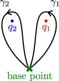
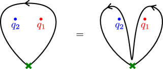
(a)		(b)

Figure -1019: To define the monodromy of a configuration unambiguously, one needs to fix a base point (shown as “$\boldsymbol{\times}$​”) with the value of the moduli there, $M$, and give monodromies of $M$ with respect to the basis of paths which start and end on the base point. (a): an example configuration with a base point and two paths $\gamma_{1}$ and $\gamma_{2}$ going around charges with monodromies $M\to Mq_{1}$ and $M\to Mq_{2}$, respectively. (b): a path going around both charges corresponds to monodromy $Mq_{1}\to Mq_{1}\cdot q_{1}^{-1}q_{2}q_{1}.$ See text for more detail.

If we know the monodromies for a basis of 1-cycles, it is possible to determine the monodromy along any paths. For example, in Fig. -1019(a), we have a configuration with two charges with individual monodromies $q_{1}$ and $q_{2}$ along paths $\gamma_{1}$ and $\gamma_{2}$, respectively. Let us consider going around both charges at the same time as shown in Fig. -1019(b). By homotopically deforming the path as shown, we see that this path is the composition of $\gamma_{1}$ and $\gamma_{2}$, which we denote by $\gamma_{2}\gamma_{1}$. As we move along $\gamma_{1}$, we get the monodromy $M\to Mq_{1}$ by definition. When we further go along $\gamma_{2}$, we are starting with the moduli $\tilde{M}=Mq_{1}$. Therefore, using (3.2), the moduli now transform as $Mq_{1}\to Mq_{1}\cdot q_{1}^{-1}q_{2}q_{1}$. Namely, the monodromy for going around both $q_{1},q_{2}$ at the same time is $M\to Mq_{1}\cdot q_{1}^{-1}q_{2}q_{1}=Mq_{1}^{-1}(q_{1}q_{2})q_{1}=Mq_{2}q_{1}$.

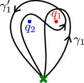
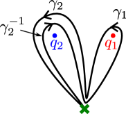
(a) Two paths going around $q_{1}$.	(b) Path $\gamma^{\prime}_{1}$ is equal to $\gamma_{2}\gamma_{1}\gamma_{2}^{-1}$.
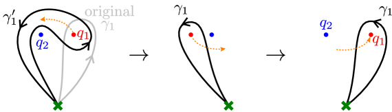
(c) Interchanging charges will change paths.

Figure -1018: The monodromy charge depends on the choice of paths with respect to which to measure the monodromy. See text for detail.

To define monodromy charge unambiguously, it is important to fix once and for all the paths along which to measure monodromy, not just the base point. For example, in the present configuration, $\gamma_{1}$ is not the only path that includes the base point and goes around $q_{1}$. In Fig. -1018(a), we presented one other example denoted by $\gamma_{1}^{\prime}$. The monodromy along $\gamma_{1}^{\prime}$ can be easily computed to be $M\to Mq_{2}q_{1}q_{2}^{-1}$, by noting that path $\gamma_{1}^{\prime}$ is equal to $\gamma_{2}\gamma_{1}\gamma_{2}^{-1}$ as shown in Fig. -1018(b). In general, homotopically different paths that encircle the same brane give different monodromy charges that are related to each other by conjugation.

There is an related subtlety when we move one charge around another. Let us consider moving charge $q_{1}$ around charge $q_{2}$ counterclockwise, as shown in Fig. -1018(c). Before the move, we have path $\gamma_{1}$ with monodromy $M\to Mq_{1}$ and path $\gamma_{1}^{\prime}$ with monodromy $M\to Mq_{2}q_{1}q_{2}^{-1}$ (see the left panel of the Figure). After the move, the system looks as if it went back to the original configuration, with the original $\gamma_{1}^{\prime}$ changed into a “new $\gamma_{1}$” (the right panel). However, because monodromy living in the discrete space $G({\mathbb{Z}})$ cannot change under continuous deformation of the path, the monodromy associated with this new “new $\gamma_{1}$” is given by $M\to Mq_{2}q_{1}q_{2}^{-1}$, not the original $M\to Mq_{1}$. So, every time we move a charge around another, it looks as if the charge measured by path $\gamma_{1}$ jumps. This is happening because we are choosing different paths to measure the charge and, if we stick to the original path by following its continuous deformation, the monodromy charge remains the same. This point is important in understanding charge conservation in the presence of exotic branes, as we will see in the next subsection.

Let us ask a question of what charges exist in a fixed $U$-duality frame. Let us start from the situation given in (3.1), where a brane with monodromy $q$ exists. Furthermore, let us assume that we can arrange codimension-2 branes so that the moduli $M$ at infinity tends to a constant value, without a non-trivial monodromy. We can achieve this by having multiple codimension-2 branes with canceling monodromies or curling up branes as we will discuss in section 5. After dualization, one has a brane with monodromy $\tilde{q}$ as in (3.2) and, at the same time, the value of the moduli at infinity have changed to $\tilde{M}$. Now, let us change the moduli at infinity adiabatically back to the original value $M$. If the brane configuration is supersymmetric, we expect that the brane with monodromy $\tilde{q}$ survives the adiabatic process, provided that there is no wall of marginal stability. So, a brane with charge $\tilde{q}$ should exist even for the original value of the moduli $M$. Namely, if a brane with monodromy $q$ exists, branes with monodromies $\tilde{q}=U^{-1}qU$, $U\in G({\mathbb{Z}})$ should also exist. One caveat, however, is that this does not mean that we can generate all charges that exist in the theory by conjugation; there can be many conjugacy classes in the group $G({\mathbb{Z}})$ and we cannot generate charges in different conjugacy classes. Also, there can be non-supersymmetric configurations for which the above argument of adiabatically changing moduli does not apply.

Note that the above argument is not a very strong one. First, in a situation where we cannot make the moduli to tend to a constant value at infinity, the conjugated charges do not have to exist. For example, if there is a single charged particle $q$ in 3D, then the moduli has the monodromy $M\to Mq$ even at infinity and the above argument does not apply. Also, if a wall of marginal stability exists, the above argument can fail.

As a simple example, consider a D7-brane in Type IIB superstring. Around it, there is a non-trivial monodromy of the $SL(2,{\mathbb{Z}})$ duality given by

$$T=\begin{pmatrix}1&1\\ 0&1\end{pmatrix}.$$ (3.3)

Let us conjugate this with a general $SL(2,{\mathbb{Z}})$ matrix

$$U=\begin{pmatrix}s&r\\ q&p\end{pmatrix},\qquad sp-rq=1.$$ (3.4)

The conjugated charge is

$$\tilde{T}=U^{-1}TU=\begin{pmatrix}1+pq&p^{2}\\ -q^{2}&1-pq\end{pmatrix},$$ (3.5)

which is the monodromy of the standard $(p,q)$ 7-brane. So, if the assumptions we made above are true, there should also exist $(p,q)$ 7-branes with $p,q$ coprime. If we further assume the existence of a bound state of $N$ 7-branes with monodromy

$$T^{N}=\begin{pmatrix}1&N\\ 0&1\end{pmatrix}.$$ (3.6)

for all $N\in{\mathbb{Z}}$, then there should exist 7-branes the monodromy

$$\tilde{T}^{N}=U^{-1}T^{N}U=\begin{pmatrix}1+Npq&Np^{2}\\ -Nq^{2}&1-Npq\end{pmatrix}.$$ (3.7)

Note that the monodromy matrix thus obtained has always $\mathop{\mathrm{tr}}\nolimits(\tilde{T}^{N})=2$. Because trace (partly) characterizes the conjugacy classes of $SL(2,{\mathbb{Z}})$, we cannot reach objects whose monodromy matrices have trace different from $2$ by starting from a $(p,q)$ 7-brane (for classification of $SL(2,{\mathbb{Z}})$ conjugacy classes, see [14, 15]). It is not clear whether in string theory there exist 7-branes whose monodromy is not in the trace-2 conjugacy class. Note that, although the orientifold 7-plane in Type IIB superstring has a monodromy which is not in the trace-2 class, in F-theory it is represented by a bound state of $(p,q)$ 7-branes, each of which is in the trace-2 class [57, 58]. However, it is known that supersymmetric 7-brane solutions with general conjugacy classes (“Q7-branes”) do exist at the level of classical supergravity [59, 60, 61]. The meaning of such solutions in string theory is not clear.

3.2 Monodromies and charge conservation

In the presence of an exotic brane with a non-trivial $U$-duality monodromy, moving a second brane around it will $U$-dualize the second brane into a different brane. Therefore, it appears that the associated brane charge is not conserved in the presence of an exotic brane. Here we demonstrate, based on explicit examples, that this is not the case and charges are actually conserved even in such situations, if we use the appropriate notion of charge.

More precisely, the question is the following. An exotic brane is a codimension-2 brane in $d$ dimensions and there is a non-trivial monodromy of $d$ dimensional scalars around it. Now, introduce a second object which is charged under some gauge field in $d$ dimensions. It sometimes happens that moving the second object around the codimension-2 exotic brane apparently induces a new charge. We would like to understand how this phenomenon is consistent with charge conservation.

3.2.1 Charge conservation and Page charge

To start the discussion with, let us consider a D7-brane along $\psi 456789$ directions. Here, we take $456789$ to be compact directions with period $2\pi l_{s}$. $\psi$ can be either a compactified direction or the direction along a contractible circle in non-compact ${\mathbb{R}}^{3}_{123}$. The first case is simpler but the transverse spacetime directions will not be asymptotically flat ${\mathbb{R}}^{2}$ once backreaction is taken into account, as will be discussed in section 4. In the second case, the transverse spacetime remains asymptotically flat ${\mathbb{R}}^{3}$ even if backreacted, as will be studied in section 5. See Figure -1017 for a schematic description of the configurations. In the second case, the D7-brane can either be a static configuration supported by something (e.g. by a supertube effect, as will be studied in section 5) or just an instantaneous configuration which will collapse eventually.

Figure -1017: A D7-brane along $\psi 456789$ directions, with $\psi$ being (a) a compactified direction and (b) a direction along a contractible circle.

In either case, the D7-brane is a codimension-2 object already in $d=10$ dimensions and, around it, there is a non-trivial $SL(2,{\mathbb{Z}})$ monodromy described by the matrix $q=(\begin{smallmatrix}1&1\\ 0&1\end{smallmatrix})$. So, the scalar $\tau=C^{(0)}+ie^{-\Phi}$ has the monodromy $\tau\to\tau+1$.

Now, add to this configuration an NS5-brane along $56789$ directions and consider moving it around the D7-brane. The NS5-brane is magnetically charged under the gauge field $B^{(2)}$. Because $A^{T}=(C^{(2)},B^{(2)})^{T}$ is a doublet under $SL(2,{\mathbb{Z}})$ transforming as $A\to qA$, $C^{(2)}$ changes as $C^{(2)}\to C^{(2)}+B^{(2)}$ as we go around the D7. Because the integral of $dC^{(2)}$ measures D5-brane charge, this means that moving an NS5 around a D7 produces D5-branes; see Figure -1016. Let us write this as

$$\rm D7(\psi 456789):\quad NS5(56789)\to NS5(56789)+D5(56789).$$ (3.8)

Another way to see that $C^{(0)}$ induces D5-brane charge on the NS5-brane is as follows. By the Wess–Zumino term in the D-brane worldvolume action, non-vanishing $B^{(2)}_{89}\neq 0$ induces D3(567) charge on the D5(56789) worldvolume. The $S$-dual of this statement is that $C^{(2)}_{89}$ induces D3(567) on NS5(56789). Further by $T_{89}$, we see that $C^{(0)}$ induces D5(56789) on NS5(56789).

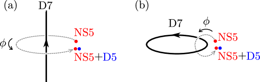
Figure -1016: Moving an NS5-brane around a D7-brane appears to produce D5-branes.

By taking $S$, $T_{89}$, $S$, and then $T_{567}$ dualities of (3.8), we see that moving a D0 around a $5^{2}_{2}$ produces D2-brane charge:

$$\rm 5_{2}^{2}(\psi 4567;89):\quad D0\stackrel{{\scriptstyle?}}{{\to}}D0+D2(89),$$ (3.9)

where the D0 is smeared along 456789 directions and the D2(89) is smeared along 4567 directions. We have put a question mark in (3.9) because we will later question this process.

Further by taking $T_{89}$ of (3.9), we see that moving a D2 around an NS5 produces D0 charge:

$$\rm NS5(\psi 4567):\quad D2(89)\to D2(89)+D0,$$ (3.10)

where, again, branes are smeared along transverse directions within the compact $456789$ directions. The NS5($\psi$4567)-brane can be thought of as a codimension-2 object in 8D if we compactify the 10D theory on $T^{2}_{89}$.

Let us study the above processes (3.8)–(3.10), in which brane charges do not appear to be conserved, and examine in what sense they can actually be conserved.

We begin with (3.10) as the easiest situation to study, although the NS5($\psi 4567$) is not an exotic brane. Because the $89$ directions are compactified, from the viewpoint of the non-compact directions ($123$ or $1234$, depending on the situations (a), (b) of Fig. -1017), the NS5($\psi 4567$) is a codimension-2 object. The charge of the NS5($\psi 4567$)-brane is measured by

$$Q^{\text{NS5}}={1\over 2\pi(2\pi l_{s})^{2}}\int_{\phi 89}H^{(3)}={1\over 2\pi}[B_{89}^{(2)}]^{\phi=2\pi}_{\phi=0}\equiv{1\over 2\pi}\Delta B_{89}^{(2)},$$ (3.11)

where $\phi$ is an angular direction encircling the NS5-brane in the non-compact space (see Figure -1016). This means that $B_{89}^{(2)}$ increases by $\Delta B_{89}^{(2)}=2\pi Q^{\text{NS5}}$ as we go around the NS5. Now, the D2-brane Wess–Zumino coupling

$$S^{\text{D2,WZ}}={1\over(2\pi)^{2}l_{s}^{3}}\int(C^{(3)}-B^{(2)}\wedge C^{(1)})$$ (3.12)

implies that moving a D2(89) around the NS5 will induce D0-charge

$$\Delta Q^{\text{D0,bs}}={1\over(2\pi l_{s})^{2}}\int\Delta B^{(2)}=\Delta B_{89}^{(2)}=2\pi Q^{\text{NS5}}.$$ (3.13)

The superscript “bs” will be explained below. In (3.12), we assumed that the Chan–Paton (Born–Infeld) gauge field strength $F^{(2)}$ in the D-brane worldvolume vanishes. Therefore, it appears that D0 charge $Q^{\text{D0,bs}}$ is not conserved and increases by (3.13) every time we move the D2 around the NS5.

However, recall that, as discussed in [37], there are multiple notions of charge and we should be careful about what charge we are talking about. Brane source charge is gauge-invariant but not conserved, whereas Page charge is conserved and gauge-invariant under small gauge transformation. Page charge changes under global gauge transformation, but global gauge transformation changes the state of the system and charge does not have to remain the same under it in the first place. Moreover, it is Page charge that is quantized and appears in the asymptotic super-Poincaré algebra as central charge [37]. So, if we want to discuss charge conservation, it is Page charge that we should consider, not brane source charge. We discuss brane source and Page charges in Appendix D. Here, we only use the results for the expression of brane source and Page charges from there and refer the reader to the appendix for details.

D-brane source current is obtained simply by varying the D-brane action (3.12) with respect to RR potential $C$, as discussed in Appendix D. Therefore, D-brane source charge includes the D-brane charge induced by the spacetime $B^{(2)}$ field, and $Q^{\text{D0,bs}}$ in (3.13) is brane source charge; that is why the superscript “bs”. On the other hand, D-brane Page charge is obtained from brane source charge precisely by subtracting the charge induced by $B^{(2)}$. Therefore, for Page charge, (3.13) is modified to

$$\Delta Q^{\text{D0,Page}}=0.$$ (3.14)

Namely, even if we move D2 around NS5, no Page D0 charge is induced and it is actually conserved.

Now let us turn to the process (3.8). Although the D7-brane has codimension 2, it is not quite exotic in that the monodromy around it does not involve metric; it is just an additive shift of $C^{(0)}$. The analysis of this process is similar to that of (3.10). Namely, although it appears that D5-brane charge is induced on the NS5-brane by spacetime RR potentials $C$, as discussed in Appendix D, D5-brane Page charge is defined by subtracting such induced charge. Therefore, in this case, there is no D5-brane charge induced, i.e.,

$$\Delta Q^{\text{D5,Page}}=0.$$ (3.15)

Even if we move NS5 around D7, no Page D5 charge is induced and charge is conserved.

Finally, let us consider the process (3.9) in which the exotic brane $5^{2}_{2}$ is involved. First of all, we immediately notice that D2-charge being induced on a D0 is strange, because the D0-brane Wess–Zumino term

$$S^{\text{D0,WZ}}={1\over l_{s}}\int C^{(1)}$$ (3.16)

does not involve $C^{(3)}$ and there is no way to induce D2 charge on a D0. The mistake we made is the following. The D0-brane charge on the right hand side of (3.10), which we confirmed is induced, is brane source charge. Actually, brane source charge do not transform covariantly under duality transformations, and therefore the existence of induced D0-brane source charge in the duality frame (3.10) does not imply that D2-brane source charge is induced in the duality frame (3.8) as we naively presumed. Therefore, in order to study the charge in (3.8), we need instead a notion of charge that transforms covariantly under duality.

It turns out to that the charge that transformscovariantly under duality is Page charge. This can be seen as follows. Let us focus on the $T$-duality transformation that we performed in going between (3.9) and (3.10). If we compactify the 10D theory on $T^{2}_{89}$ down to 8D, we have $T$-duality group $SO(2,2,{\mathbb{Z}})=SL(2,{\mathbb{Z}})_{\tau}\times SL(2,{\mathbb{Z}})_{\rho}$. Here, $\tau,\rho$ are 8D moduli scalars defined by

$$\rho =B^{(2)}_{89}+i\det\nolimits^{1/2}G_{ab},\qquad G_{ab}={\rho_{2}\over\tau_{2}}\begin{pmatrix}1&\tau_{1}\\ \tau_{1}&|\tau|^{2}\end{pmatrix},\qquad a,b=8,9$$ (3.17)

and transform in the standard way under respective $SL(2,{\mathbb{Z}})$ factors; namely,

$$\rho\to\rho^{\prime}={a\rho+b\over c\rho+d},\qquad\begin{pmatrix}a&b\\ c&d\end{pmatrix}\in SL(2,{\mathbb{Z}})_{\rho}~{},$$ (3.18)

and likewise for $\tau$ and $SL(2,{\mathbb{Z}})_{\tau}$. As we will study in detail in section 4, NS5($\psi 4567$) and $5^{2}_{2}(\psi 4567,89)$ can be both thought of as codimension-2 branes in 8D with non-trivial monodromies for the scalar $\rho$, but no such details are necessary for the current discussion. The $T$-duality transformation that we performed in going between (3.9) and (3.10) belongs to $SL(2,{\mathbb{Z}})_{\rho}$ [63]. Upon reducing to 8D, the D0 and D2(89)-branes both become 0-branes, and the 10D RR potentials $C_{\mu}$ and $C_{89\mu}$ ($\mu=0,\dots,7$) that they couple to reduce to 8D 1-forms, ${\cal C}_{\alpha\mu}$ ($\alpha=1,2$), which form a doublet under $SL(2,{\mathbb{Z}})_{\rho}$ [6, 64]. Ref. [64] showed that the covariant field ${\cal C}_{\alpha\mu}$ in 8D is related to $C_{\mu}$ and $C_{89\mu}$ by

$${\cal C}_{1,\mu}=C_{\mu},\qquad{\cal C}_{2,\mu}=C_{89\mu}-B_{89}C_{\mu}.$$ (3.19)

If we define charge currents covariant under the $T$-duality group by variation of the action with respect to ${\cal C}_{\alpha\mu}$, then, using the relation

$${\delta\over\delta{\cal C}_{1,\mu}}={\delta\over\delta C_{\mu}}+B_{89}{\delta\over\delta C_{89\mu}},\qquad{\delta\over\delta{\cal C}_{2\mu}}={\delta\over\delta C_{89\mu}},$$ (3.20)

we can show that the charges associated with ${\cal C}_{\mu\alpha}$ are related to the brane source charges as

$${\cal Q}^{\alpha=1}=Q^{\rm D0,bs}+B_{89}Q^{\rm D2(89),bs},\qquad{\cal Q}^{\alpha=2}=Q^{\rm D2(89),bs},$$ (3.21)

where the volume of $T^{2}_{89}$ is $(2\pi l_{s})^{2}$. ${\cal Q}^{\alpha=1}$ is D0-brane source charge minus the one induced by the $B$-field on the D2-brane worldvolume. This is nothing but Page charge for the D0-brane.

So, Page charge covariantly transforms under $T$-duality transformation. In the duality frame (3.10), we have shown that D0 Page charge is conserved. By $T$-dualizing to the present duality frame (3.9), this automatically implies that D2 Page charge is conserved. The apparent non-conservation of D2-brane charge in (3.10) was simply because we were looking at a wrong notion of charge inappropriate to discuss duality transformation and charge conservation.

This argument is valid for any systems which are related to the above configuration by $T$-duality. Namely, as long as one measures Page charge, charges are always conserved. Brane source charge, on the other hand, is not conserved, but that does not contradict with charge conservation. We expect that this holds true generally, not just in the examples we considered. Namely, even in the presence of exotic scalar monodromies, brane Page charges are always unambiguously defined and conserved.

It would be interesting to show this in full generality in a more systematic way. In particular, it would be desirable to generalize the result of Ref. [64] to $U$-duality transformations. Because Page charge is the central charge that appears in the asymptotic algebra and transform covariantly under $U$-duality, this would amount to finding explicit expressions for Page charges that transform covariantly under $U$-duality.

3.2.2 Monodromies and Page charge

We thus showed that, as long as we use Page charge to define charge, there is no induced charge even when one moves a charge around an exotic brane, around which there is non-trivial $U$-monodromy. We also argued that, because Page charges transform covariantly under $U$-duality, the conservation of Page charge must hold in any frames.

But there is an apparent tension here. On one hand, we said that Page charge remain the same even when we go around an exotic brane around which there is $U$-duality monodromy. On the other hand, we said that Page charges transform covariantly under $U$-duality. How can the two statements be consistent with each other?

The resolution is closely related to the subtlety in defining monodromy charges that we discussed in section 3.1. As we discussed there, unambiguously defining monodromies requires that we fix a base point and the value of moduli at that point, once and for all, and that we measure monodromy with respect to them. A similar consideration is needed when defining Page charge. Page charge involves an integral of form fields around certain cycles that enclose the object in question. However, in the presence of exotic branes, those form fields themselves are also not globally well-defined. To define all quantities consistently, we need to choose a base point $P$ plus a choice of moduli and form fields at $P$. One can then follow the moduli and form fields continuously along any path that does not intersect the exotic brane. Namely, Page charge should properly be defined as the integral over a cycle that contains the point $P$, where the form fields and moduli take the given values $M$ and $(B,C)$ respectively, and such that moduli and form fields are continuous everywhere along the cycle. The cycle is not allowed to intersect the exotic brane.

Figure -1015: Defining Page charges in the presence of exotic branes with non-trivial monodromies requires that we fix a base point $P$ (denoted “$\times$”) along with the values of moduli $M$ and form fields $(B,C)$ there, and measure the charge with respect to them. Continuously deforming the cycle to measure charge does not change the charge. However, there can be multiple, non-equivalent cycles

In Fig. -1015(a), we described a situation where we measure Page charge of a brane sitting near the base point $P$ by integrating a form field through a cycle $\gamma$ that encloses the brane and goes through $P$. If we move the brane and at the same time continuously deform $\gamma$ so that it always goes through $P$ and does not intersect the exotic brane, Page charge does not change as we have explicitly demonstrated in section 3.2.2 above. We described this process in Fig. -1015(b).

With this definition of Page charge, it is still not unique, as there can be different topological types of cycles which one can use to compute it. Because cycles are not allowed to intersect the exotic brane, not all cycles can be continuously deformed. But cycles that can be continuously deformed into one another will give rise to the same Page charge. This should be the case since Page charge is quantized. If we take a path that encircles the exotic brane and comes back to the original base point $P$, the fields will undergo a monodromy and be mapped into a $U$-dual version of themselves. Thus, different topological types of charges will give rise to different Page charges that are related to each other through $U$-dualities.

In Fig. -1015(c), we described a situation where we have moved the brane once around the exotic brane and brought it back near the base point $P$. Besides cycle $\gamma$ that now has a “tail” going around the exotic brane, there is another cycle $\gamma^{\prime}$ that goes through $P$ and encloses the brane but does not go around the exotic brane. If we use $\gamma$ to measure Page charge, we get the same answer as the one measured in Fig. -1015(a). On the other hand, if we use $\gamma^{\prime}$ to measure Page charge, we get the $U$-dual version. There is no contradiction here because the two cycles $\gamma$ and $\gamma^{\prime}$ cannot be deformed into each other without intersecting the exotic brane; they measure physically different charges.

Now the puzzle raised at the beginning of this section 3.2.2 is resolved. When we said in section 3.2.1 that Page charge is conserved, we meant that the Page charge measured by cycle $\gamma$ is unchanged even if we move the brane around the exotic brane along with the cycle that encloses it. This is what we must do physically, because when we talk about charge conservation we should adopt one notion of charge and stick to it as we continuously change the configuration. On the other hand, the fact that Page charges transform covariantly under $U$-duality is not related to such continuous deformation, and there is no contradiction here.

3.3 Number of charges

As we discussed above, the charge of a codimension-2 brane is characterized by the monodromy around it. Since the monodromy matrix $q$ is an element of the discrete non-Abelian “lattice” $G({\mathbb{Z}})$, it does not really make sense to ask how many different charges there are, in contrast to the case of an ordinary charge lattice ${\mathbb{Z}}^{n}$ where one can say that there are $n$ different charges. However, to get a qualitative idea, we can replace $G({\mathbb{Z}})$ by the continuous group $G({\mathbb{R}})$ and study the dimension of the (now continuous) space of possible charges. This is expected to be the dimension of the space of charges that we see in the classical limit where the charges are large.

There are multiple notions that one can mean by the number of charges. In toroidal compactifications, we have a scalar moduli space of the form ${\cal M}=H({\mathbb{R}})\backslash G({\mathbb{R}})/G({\mathbb{Z}})$ whose isometry group is $G({\mathbb{R}})$. Since $G({\mathbb{R}})$ has

$$m\equiv\mathop{\mathrm{dim}}\nolimits G$$ (3.22)

generators, there are $m$ associated conserved Noether currents in the theory. In this sense, the number of charges that are in principle possible to occur in the theory is $m$. In the 3D theory, we have $G=E_{8(8)}$ and $m=248$.

If one could introduce a dual $(d-2)$-form gauge field for each of these $m$ currents, it would seem like there are $m$ different codimension-2 branes with different charges. However, as is manifest in Table 2 for $d=3$ and in Tables 6 and 7 for $d>3$, there are only

$$h\equiv\mathop{\mathrm{dim}}\nolimits G-\mathop{\mathrm{rank}}\nolimits G<m$$ (3.23)

branes that can be obtained by $U$-dualizing standard half-supersymmetric branes such as D7-branes. For example, in the $d=3$ case, $h=240$ ($<m=248$), and these are the point particle states listed in Table 2. This discrepancy between $m$ and $h$ is understood as follows [65, 66, 67]. Although there are $m$ gauge fields, only $h$ of them couple to 1/2-BPS branes. More precisely, if one tries to construct a $U$-duality and gauge invariant Wess–Zumino coupling of a possible brane to the gauge fields, it is possible to do so preserving half of supersymmetry only for $h$ gauge fields out of $m$, and these $h$ branes are in the $U$-duality orbit of the standard 1/2-BPS branes. In this sense, $h$ is the number of fundamental 1/2-BPS codimension-2 branes allowed in string theory. At the time of writing, it is not understood whether there exist states in string theory that couple to the remaining $m-h$ gauge fields. For counting of 1/2-BPS branes based on an $E_{11}$ group theoretical argument, see [43].

Yet another other notion that one may associate with the number of charges is the dimension of the $U$-duality orbit of a brane. A general analysis on the dimension of the orbits of BPS configurations in string theory was done in [68] for codimension $>2$ branes. For codimension-2 branes, such an analysis was done [7] and later by [67] along the line of [68]. Here, we repeat the analysis of [7], including some details omitted there. Let us start from a given charge $q\in G({\mathbb{R}})$. Using ${\cal Q}\in g({\mathbb{R}})$, where $g({\mathbb{R}})$ is the Lie algebra of $G({\mathbb{R}})$, we can write $q$ as $q=e^{{\cal Q}}$. In particular, if we consider 1/2 BPS objects such as D7-branes, the matrix is nilpotent, ${\cal Q}^{2}=0$, and hence $q=1+{\cal Q}$. Now, generate a new charge by conjugation by $U=e^{\epsilon t}\approx 1+\epsilon t$ where $t\in g({\mathbb{R}})$ and $\epsilon$ is infinitesimal. The new charge matrix is $\tilde{q}=U^{-1}qU\approx q+\epsilon\,[{\cal Q},t]$. So, the number of different charges is given by $\mathop{\mathrm{dim}}\nolimits g$ minus the dimension of the stabilizer subspace $\{[{\cal Q},t]=0\,|\,t\in g({\mathbb{R}})\}$. This is given as follows. First, we find an $sl(2)$ subalgebra in which ${\cal Q}$ is the raising operator. Then, decompose the adjoint representation of $g({\mathbb{R}})$ into $sl(2)$ representations as

$${\rm adj}=\bigoplus_{k=1}^{d}({\bf 2j_{k}+1})$$ (3.24)

where $d$ is the number of representations appearing in the decomposition. Since ${\cal Q}$ acts effectively on all states in each $sl(2)$ representation except for the highest spin state, we find that the dimension of the orbit, $b$, is

$$b=\mathop{\rm dim}g-d.$$ (3.25)

In the 3D case where $G=E_{8(8)}$, the adjoint representation decomposes as ${\bf 248}={\bf 3}+56\cdot{\bf 2}+133\cdot{\bf 1}$, and therefore $b=248-(1+56+133)=58$. This number agrees with the one obtained in [67] by a slightly different argument. In the last column of Table 6, we listed the values of $b$ in various dimensions.

4 Supergravity description of exotic states

In this section, we study supergravity solutions corresponding to exotic branes. In higher dimensions, they correspond to infinitely long defects in spacetime, around which there are non-geometric monodromies. These solutions are not new, but our focus will be on their exotic non-geometric aspects.

4.1 An example: the supergravity solution for $5^{2}_{2}$

To demonstrate that exotic branes are non-geometric objects, let us compute the supergravity solutions for them and analyze the structure. Using the duality rules shown in Tables 3–5, it is straightforward to start with any known standard brane backgrounds, act by supergravity duality transformation on them, and obtain the background for exotic branes. Here, as an example, let us compute the metric for $5^{2}_{2}$ by $T$-dualizing the KK monopole metric transverse to its worldvolume (cf. (2.8)). A simplified version of the following analysis was given in [7].

The metric for KK monopoles wrapped on compact $345679$ directions, with $x^{9}$ being the special circle (namely, they are $5^{1}_{2}(34567,9)$), placed at ${\bf x}={\bf x}_{p}$ in the transverse space ${\mathbb{R}}^{3}_{128}$, is

$$\begin{split}ds^{2}&=dx_{034567}^{2}+Hdx_{128}^{2}+H^{-1}(dx^{9}+\omega)^{2},\qquad e^{2\Phi}=1,\\ H&=1+\sum_{p}H_{p},\qquad H_{p}={R_{9}\over 2|{\bf x}-{\bf x}_{p}|},\end{split}$$ (4.1)

where the 1-from $\omega$ satisfies

$$d\omega=*_{3}dH$$ (4.2)

and $R_{9}$ is the radius of the $x^{9}$ direction. Also, $dx_{034567}^{2}=-(dx^{0})^{2}+(dx^{3})^{2}+\dots+(dx^{7})^{2}$ and $dx_{128}^{2}=(dx^{1})^{2}+(dx^{2})^{2}+(dx^{8})^{2}$. The labeling of the coordinates is slightly perverse for later convenience. This solution preserves half of supersymmetry. In order to be able to $T$-dualize along a transverse direction, let us compactify $x^{8}$, which is the same as arraying centers at intervals of $2\pi\tilde{R}_{8}$ along $x^{8}$. So,

$$H =1+\sum_{n\in{\mathbb{Z}}}{R_{9}\over 2\sqrt{r^{2}+(x^{3}-2\pi\tilde{R}_{8}n)^{2}}}\approx 1+\sigma\log{\Lambda+\sqrt{r^{2}+\Lambda^{2}}\over r},\qquad\sigma\equiv{R_{9}\over 2\pi\tilde{R}_{8}},$$ (4.3)

where we took a cylindrical coordinate system

$$ds_{128}^{2}=dr^{2}+r^{2}d\theta^{2}+(dx^{8})^{2}.$$ (4.4)

We approximated the sum in (4.4) by an integral and introduced a cutoff $\Lambda$ to make it convergent. The approximation is valid for $r\gg\tilde{R}_{8}$. Such computations of arraying centers were done in [69, 3]. We could have done the summation exactly [70] but the above approximation is sufficient for our purposes. $H$ in (4.3) diverges as we send $\Lambda\to\infty$, but this can be formally shifted away by introducing a “renormalization scale” $\mu$ and writing

$$H(r)=h_{0}+\sigma\log{\mu\over r}$$ (4.5)

where $h_{0}$ is a “bare” quantity which diverges in the $\Lambda\to\infty$ limit. When $H$ is given by (4.5), eq. (4.1) gives $\omega=-\sigma\theta\,dx^{8}$. The log divergence of $H$ implies that such an infinitely long codimension-2 object is ill-defined as a stand-alone object. In physically sensible configurations, this must be regularized either by taking a suitable superposition of codimension-2 objects [27] or, as we will do later, by considering instead a configuration which is of higher codimension at long distance. So, the present analysis should be regarded as for illustration purposes only.

Now let us take $T$-duality along $x^{8}$. By the standard Buscher rule, we obtain the metric and other fields for $5^{2}_{2}(34567,89)$:

$$ds^{2}_{\text{10,str}} =H\,\,(dr^{2}+r^{2}d\theta^{2})+HK^{-1}dx_{89}^{2}+dx_{034567}^{2},$$

$$e^{2\Phi} =HK^{-1},\qquad B^{(2)}=-K^{-1}{\theta\sigma}dx^{8}\wedge dx^{9},\qquad B^{(6)}=-H^{-1}Kdx^{0}\wedge dx^{3}\wedge\cdots dx^{7},$$

$$K \equiv H^{2}+\sigma^{2}\theta^{2}.$$ (4.6)

In terms of the radii in this frame,

$$\sigma={R_{8}R_{9}\over 2\pi{\alpha^{\prime}}}.$$ (4.7)

Such metric of exotic branes has been written down in the literature in various papers; some early work includes [3, 71] and more recent papers include [42, 43, 44]. However, it does not appear to have been discussed in the context of $U$-folds. Although we arrived at the $5^{2}_{2}$ solution by arraying (smearing) KK monopoles and $T$-dualizing it, which one might find uncomfortable with, we could have obtained it without arraying by taking a different route, e.g., by starting with a D7-brane metric and dualizing it [42, 45]. We will derive the same solution (actually its generalizations) again in section 4.2 more directly in supergravity without using duality.

As can be seen from (4.6), as we go around the $5^{2}_{2}$-brane at $r=0$ by changing $\theta=0$ to $2\pi$, the size of the 8-9 torus does not come back to itself:

$$\begin{split}\theta=0&:\quad G_{88}=G_{99}=H^{-1},\\ \theta=2\pi&:\quad G_{88}=G_{99}={H\over H^{2}+(2\pi\sigma)^{2}}.\end{split}$$ (4.8)

Therefore, indeed, the exotic $5^{2}_{2}$-brane has a non-geometric spacetime around it. This non-geometric spacetime can be understood as a $T$-fold as follows. If we package the 8-9 part of the metric and $B$-field in a $4\times 4$ matrix [72]

$$M=\begin{pmatrix}G^{-1}&G^{-1}B\\ -BG^{-1}&G-BG^{-1}B\end{pmatrix}$$ (4.9)

then the $SO(2,2)$ $T$-duality transformation matrix $\Omega$ satisfying

$$\Omega^{t}\eta\Omega=\eta,\qquad\eta=\begin{pmatrix}0&{\bf 1}_{2}\\ {\bf 1}_{2}&0\end{pmatrix},$$ (4.10)

acts on $M$ as

$$M\to M^{\prime}=\Omega^{t}M\Omega.$$ (4.11)

It is easy to see that the matrix

$$\Omega=\left(\begin{matrix}{\bf 1}_{2}&0\\ 2\pi\sigma&{\bf 1}_{2}\end{matrix}\right)$$ (4.12)

relates the $\theta=0,2\pi$ configurations in (4.8). Namely, $5^{2}_{2}$ is a non-geometric $T$-fold with the monodromy $\Omega$.

Another way to represent the monodromy is in terms of the $SO(2,2,{\mathbb{Z}})=SL(2,{\mathbb{Z}})_{\tau}\times SL(2,{\mathbb{Z}})_{\rho}$ mentioned in section 3.2.1. Let us introduce moduli $\tau,\rho$ defined in (3.17) and take a complex coordinate $z=re^{i\theta}$. From (4.6), we can read off

$$\rho={iH-\sigma\theta\over K}={i\over h_{0}+\sigma\ln(\mu/z)},\qquad\tau=i.$$ (4.13)

So, as we go around $5^{2}_{2}$ ($z\to ze^{2\pi i}$), it is not $\rho$ but $\rho^{\prime}=-1/\rho$ that undergoes a simple shift:

$$\rho^{\prime}\to\rho^{\prime}+2\pi\sigma.$$ (4.14)

(If $\rho$ underwent a shift $\rho\to\rho+1$ as $z\to ze^{2\pi i}$ instead, the configuration would be simply an NS5(56789)-brane.) In terms of the original $\rho$, we have

$$\rho\to{a\rho+b\over c\rho+d},\qquad\begin{pmatrix}a&b\\ c&d\end{pmatrix}=\begin{pmatrix}1&0\\ -2\pi\sigma&1\end{pmatrix}.$$ (4.15)

Let us study the behavior of the $5^{2}_{2}$ metric in the string frame, (4.6), near $r=0$. Near $r=0$, the functions in (4.6) behave as

$$H\sim\sigma\ln({\mu/r}),\qquad K\sim[\sigma\ln({\mu/r})]^{2},$$ (4.16)

where we absorbed the constant $h_{0}$ into $\mu$. Therefore, the $r\to 0$ behavior of the metric is

$$ds^{2}_{\text{10,str}} \sim[\sigma\ln({\mu/r})](dr^{2}+r^{2}d\theta^{2})+[\sigma\ln({\mu/r})]^{-1}dx_{89}^{2}+dx_{034567}^{2}.$$ (4.17)

Let us introduce a new coordinate $\rho$ by

$$d\rho=\sqrt{\sigma\ln({\mu/r})}\,dr,\qquad\rho={\sqrt{\pi\sigma}\mu\over 2}\left[1-{\rm erf}\left(\sqrt{\log(\mu/r)}\right)\right]+\sqrt{\sigma\log(\mu/r)}\,r,$$ (4.18)

where

$${\rm erf}(x)={2\over\sqrt{\pi}}\int_{0}^{x}e^{-t^{2}}dt.$$ (4.19)

For $r\sim 0$, $\rho\sim 0$, the relation between $r$ and $\rho$ is simply

$$\rho\sim\sqrt{\sigma\log(\mu/r)}\,r$$ (4.20)

and therefore the metric (4.17) becomes

$$ds^{2}_{\text{10,str}} \sim d\rho^{2}+\rho^{2}d\theta^{2}+{r^{2}\over\rho^{2}}dx_{89}^{2}+dx_{034567}^{2}.$$ (4.21)

One sees that the linearly wrapped directions $x^{3,\dots,7}$ remain finite while the quadratically wrapped directions $x^{8,9}$ shrink at the position of the brane, $\rho=0$ ($r=0$). On the other hand, the metric along the transverse directions $(\rho,\theta)$ are actually flat near the brane.

Similarly, it is easy to show that the Einstein metric in 3D,

$$ds_{\text{3,Ein}}^{2}=-dt^{2}+Hdx^{2}_{12},$$ (4.22)

is also flat at $r=0$ and there is no conical deficit there. This means that the mass of the brane is not localized at $r=0$ but is spread over the space. We can compute the mass of this configuration (4.22) by the following ad hoc procedure, even though the mass of a codimension-2 object is not strictly well-defined. Let $\gamma_{ij}$ be the spatial metric for constant $t$ slices and $G_{\mu\nu}$ the Einstein tensor. We find that $\sqrt{\gamma}\,G_{0}^{0}={1\over 2}\partial_{i}^{2}\log H$. So, the energy is

$$M =-{1\over 8\pi G_{3}}\int d^{2}x\sqrt{\gamma}\,G_{0}^{0}=-{1\over 16\pi G_{3}}\int dS\cdot\nabla\log H.$$ (4.23)

If we use (4.5) and assume that $H(r=\infty)=1$, then

$$M={1\over 16\pi G_{3}}\left.\left[{{2\pi\sigma}\over H(r)}\right]\right|_{r\to\infty}={R_{3}\cdots R_{7}(R_{8}R_{9})^{2}\over g_{s}l_{s}^{9}},$$ (4.24)

as expected of a $5^{2}_{2}(34567,89)$. Here, we used $16\pi G_{3}={g_{s}^{2}l_{s}^{8}/R_{3}\cdots R_{9}}$. Although the $5^{2}_{2}$ changes the asymptotics, setting $H(r=\infty)=1$ effectively puts it in an asymptotically flat space and allows us to compute its mass.

Because the $5^{2}_{2}$ background (4.6) has non-vanishing NSNS $B$-field, it is natural to ask if it carries F1 and/or NS5 charges. First, it does not carry F1 charge, because $H^{(7)}=dB^{(6)}$ has no purely spatial component. On the other hand, since $H^{(3)}=dB^{(2)}$ has non-vanishing spatial components, it appears that there is non-vanishing NS5(34567)-brane charge in this solution. However, as one can easily derive from (4.6), $H^{(3)}$ is not single valued as $\theta\to\theta+2\pi$. Therefore, it does not make sense to integrate the flux $H^{(3)}$ around the $5^{2}_{2}$ to measure the NS5 charge; the integral is not well-defined and its value changes as one goes around the $5^{2}_{2}$. This state of matter can be understood by noting that the pair of charges (NS5(34567), $5_{2}^{2}$(34567,89)) can be $U$-dualized to (D7(3456789), $7_{3}$(3456789)) in Type IIB. Because $7_{3}$ is $S$-dual of D7, the axio-dilaton $\tau=C^{(0)}+ie^{-\Phi}$ behaves around $7_{3}$ as $\tau(r,\theta)=-{2\pi i/\log z}$ where $z=re^{i\theta}$. Therefore, around a $7_{3}$-brane, the RR 0-form is given by $C^{(0)}=-2\pi\theta/[(\log r)^{2}+\theta^{2}]$. One can define the 1-from flux $G^{(1)}=dC^{(0)}$ and try to define the D7-brane charge by the integral $\oint G^{(1)}=[C^{(0)}]^{\theta+2\pi}_{\theta}$, but this is nonsensical because this integral depends on $\theta$. The only sensible way to define the charge of $(p,q)$ 7-brane is via the monodromy matrix (3.5). Similarly, the only sensible way to define the (NS5,$5^{2}_{2}$) charge is by the monodromy matrix, which in the current situation is (4.12) and implies that there is no NS5 charge. We will discuss the explicit monodromy matrices of NS5 and $5^{2}_{2}$ in section 4.2.

Because only NSNS fields are excited in the solution (4.6), the $5^{2}_{2}$-brane exists in all string theories, including Type I and heterotic strings. Moreover, the tension of the $5^{2}_{2}$-brane is proportional to $g_{s}^{-2}$, just like that of the NS5-brane and KK monopole. Therefore, the solution (4.6) must represent a legitimate configuration of string theory and give an approximate description of the physics, much as the supergravity solutions of the NS5 and KK monopole do (again, with the caveat that it cannot exist as a stand-alone object). What is interesting about this $5^{2}_{2}$ background is that, because the involved duality monodromy is the perturbative $T$-duality, it should allow a string theory description in terms of a worldsheet sigma model. It would very interesting to find such a sigma model description. In particular, to derive the $5^{2}_{2}$ metric by $T$-duality, we used the Buscher rule, which is a valid prescription only at the supergravity level. In string theory, the $T$-duality rule can be corrected by stringy effects and it would be interesting to examine such effects for $5^{2}_{2}$ using sigma model. In the case of $T$-duality between NS5 and KKM, it was a non-trivial matter how the position of the NS5-brane along the direction of $T$-duality is encoded in the $T$-dual KKM background by worldsheet instanton effects [73, 74, 75] (see also [76, 77, 78]). Exactly the same issue arises in the $5^{2}_{2}$ background also and it would be interesting to understand it better.

The $5^{2}_{2}$-brane is the only exotic brane with mass proportional to $g_{s}^{-2}$ and all other exotic branes in (2.11) and (2.12) have mass proportional to $g_{s}^{-3}$ or $g_{s}^{-4}$. For example, formal applications of duality transformations on (4.6) give the following $4^{3}_{3}(3456,789)$-brane metric:

$$ds_{\rm str}^{2}=H^{1/2}K^{1/2}(dr^{2}+r^{2}d\theta^{2})+H^{-1/2}K^{1/2}dx_{03456}^{2}+H^{1/2}K^{-1/2}dx_{789}^{2}.$$ (4.25)

$H$ and $K$ are the same ones as given in (4.5) and (4.6), except that now

$$\sigma={NR_{7}R_{8}R_{9}\over 2\pi g_{s}l_{s}^{3}}.$$ (4.26)

Just as we did in (4.24), we can formally show that mass of this object is

$$M={NR_{3}\cdots R_{6}(R_{7}R_{8}R_{9})^{2}\over g_{s}^{3}l_{s}^{11}}.$$ (4.27)

One may think that such exotic branes with mass $\sim g_{s}^{-3},g_{s}^{-4}$ have too large backreaction for supergravity solutions to give a meaningful description. However, that is too quick. One can show that the $4^{3}_{3}$ solution (4.25) has no conical deficit at $r=0$, just as for $5^{2}_{2}$. This means that there is no localized energy at $r=0$ but, as is clear from the computation leading to (4.24), the energy of an exotic brane is delocalized and spread in the surrounding space over a large distance. What we mean by the mass of the exotic brane being proportional to $g_{s}^{-3}$ or $g_{s}^{-4}$ is that, if we took metrics such as (4.6) and (4.25) at face value and integrated the energy density distributed over long distances up to $r=\infty$, then the total would be proportional to $g_{s}^{-3}$ or $g_{s}^{-4}$, enough to destroy the spacetime picture. This means that the metric of a stand-alone exotic brane such as (4.6) and (4.25) should be thought of as an approximation near $r=0$ and must be replaced at some large $r$ by some other solution so that the total energy stored in space is at most $\sim g_{s}^{-2}$. This is precisely what one does in F-theory [51], where one considers a configuration of 24 $(p,q)$ 7-branes to stop the space from extending to $r=\infty$. Instead, the transverse space terminates at a finite distance and becomes a compact $S^{2}$. Note that a $(p,q)$ 7-brane is nothing but a bound state of D7-branes and $7_{3}$-branes with mass $\sim g_{s}^{-3}$. Nevertheless, the configuration has finite energy because the space is now finite; actually, the size of the transverse $S^{2}$ is a modulus and can be arbitrarily large. This clearly shows that it is too quick to regard exotic branes with nominal tension $\sim g_{s}^{-3},g_{s}^{-4}$ as physically irrelevant. To examine the physics of such heavy exotic branes, one possibility is to extend the framework of the original F-theory to geometrize the moduli space of the $U$-duality group and study the geometry of the extended spacetime, i.e. the moduli space fibered over the physical spacetime. As mentioned in section 2.5, this direction has been already undertaken in [52] followed by a spur of activity [53, 54, 55, 56, 79]. It would be desirable to revisit this with the improved understanding of exotic branes provided in the current paper.

Even if the problem of the superficial mass being proportional to $g_{s}^{-3}$, $g_{s}^{-4}$ can be evaded, it should be noted that, as exemplified by the $(p,q)$ 7-branes of F-theory, the monodromy of exotic branes involve $U$-duality and therefore the string coupling cannot generally be made small at all points in spacetime. In such cases, we should regard the supergravity solution as a qualitative guide for the physics at best. However, for protected BPS quantities, they should probably give precise predictions.

4.2 Supersymmetry analysis of $5^{2}_{2}$ solution

Being dual to the KKM solution which preserves half of supersymmetry, the exotic $5^{2}_{2}$ solution (4.6) should also preserve half of supersymmetry. It is an instructive exercise to see how this works. Because of the non-trivial duality monodromy, the Killing spinor is not single-valued around an exotic brane. Supersymmetry analyses of non-geometric solutions have already appeared in the literature; our purpose here is to only illustrate how supersymmetry is compatible with exotic $U$-duality monodromies. For example, an essentially identical but somewhat less general analysis of the supersymmetry of the $5^{2}_{2}$-brane solution was done in [42]. Ref. [46] provides a supersymmetry analysis of this system in a more general setup but from a different perspective from ours.

In Type IIA/B supergravity with purely NS background fields, the supersymmetry transformation for dilatino $\lambda$ and gravitino $\Psi_{M}$ is, respectively [80, 81],

$$\delta\lambda =\left[{1\over 2}\ooalign{\hfil/\hfil\crcr$\partial$}\Phi-{1\over 4}\ooalign{\hfil/\hfil\crcr$H$}\sigma^{3}\right]\epsilon,\qquad\delta\Psi_{M}=\left[\nabla_{M}-{1\over 8}\Gamma^{NP}H_{MNP}\sigma^{3}\right]\epsilon.$$ (4.32)

Here, the supersymmetry transformation parameter $\epsilon=\left(\begin{smallmatrix}\epsilon_{1}\\ \epsilon_{2}\end{smallmatrix}\right)$ is a doublet of Majorana–Weyl spinors $\epsilon_{1,2}$ with appropriate chirality (see Appendix B). The Pauli matrices such as $\sigma^{3}$ in (4.32) acts on the doublet index. For our convention, see Appendix A.

Although the $5^{2}_{2}$ solution we obtained by dualizing a known solution is (4.6), it is instructive to study the supersymmetry of the following more general configuration:

$$\begin{split}ds_{10}^{2}&=f^{2}\eta_{\mu\nu}dx^{\mu}dx^{\nu}+g^{2}\delta_{ij}dx^{i}dx^{j}+h^{2}\delta_{ab}dx^{a}dx^{b},\qquad H^{(3)}=H_{i}dx^{i}\wedge dx^{8}\wedge dx^{9},\\ \mu,\nu&=0,3,4,5,6,7,\qquad i,j=1,2,\qquad a,b=8,9.\end{split}$$ (4.33)

We assume that $f,g,h,H_{i}$ and $\Phi$ are functions of $x^{i}$. If we take the vielbein to be

$$e^{\hat{\mu}}_{\nu}=f\delta^{\mu}_{\nu},\qquad e^{\hat{\imath}}_{j}=g\delta^{i}_{j},\qquad e^{\hat{a}}_{b}=h\delta^{a}_{b},$$ (4.34)

then the non-vanishing components of the spin connection are

$$\omega_{\mu\hat{\nu}\hat{\imath}}=g^{-1}\eta_{\mu\nu}\partial_{i}f,\qquad\omega_{a\hat{b}\hat{\imath}}=g^{-1}\delta_{ab}\partial_{i}h,\qquad\omega_{i\hat{\jmath}\hat{k}}=g^{-1}(\delta_{ij}\partial_{k}g-\delta_{ik}\partial_{j}g).$$ (4.35)

For this configuration, the supersymmetry variation (4.32) becomes

$$\delta\lambda =\left[{1\over 2}\Gamma^{i}\partial_{i}\Phi-{1\over 4}H_{i}\Gamma^{i89}\sigma^{3}\right]\epsilon, \delta\Psi_{\mu} =\left[{1\over 2}\eta_{\mu\nu}f\partial_{i}f\Gamma^{\nu i}\right]\epsilon,$$

$$\delta\Psi_{a} =\left[{1\over 2}h\partial_{i}h\Gamma^{ai}-{1\over 4}\epsilon_{ab}H_{i}\Gamma^{bi}\sigma^{3}\right]\epsilon, \delta\Psi_{i} =\left[\partial_{i}+{1\over 2}\epsilon_{ij}g\partial_{j}g\,\Gamma^{12}-{1\over 4}H_{i}\Gamma^{89}\sigma^{3}\right]\epsilon.$$ (4.36)

We assumed that $\epsilon$ depends only on $x^{i}$. $\epsilon_{ij}$ and $\epsilon_{ab}$ are antisymmetric symbols with $\epsilon_{12}=\epsilon_{34}=1$. For the configuration (4.33) to be supersymmetric, there should exist $\epsilon$ for which all of (4.36) vanish. First, in order that $\delta\Psi_{\mu}=0$, we see that $\partial_{i}f=0$ for all $i$ and therefore we can take $f=1$ by an appropriate rescaling of $x^{\mu}$.

Next, let us look at the condition $\delta\lambda=0$, which can be written as

$$\Gamma^{\hat{\imath}}[2h^{2}\partial_{i}\Phi-H_{i}\Gamma^{\hat{8}\hat{9}}\sigma^{3}]\epsilon=0.$$ (4.37)

It is not difficult to see that this can be rewritten as a projection condition

$$(1+P)\epsilon=0,\qquad P^{2}=1,$$ (4.38)

if $\Phi$ and $h$ are related by

$$H_{i}=\pm 2\epsilon_{ij}h^{2}\partial_{j}\Phi.$$ (4.39)

The matrix $P$ is given explicitly as

$$P =\pm\Gamma^{\hat{1}\hat{2}\hat{8}\hat{9}}\sigma^{3}.$$ (4.40)

Since $\mathop{\mathrm{tr}}\nolimits P=1$, the condition (4.38) annihilates exactly one half of the components of $\epsilon$.

Because we want a 1/2-BPS configuration, the remaining conditions $\delta\Psi_{a}=0$, $\delta\Psi_{i}=0$ must give no additional constraint on the spinor $\epsilon$. The $\delta\Psi_{a}=0$ condition can be easily seen to reduce to the same condition (4.38) if we set

$$h^{-1}\partial_{i}h=\partial_{i}\Phi,\qquad\text{therefore}\qquad e^{\Phi}=h.$$ (4.41)

Finally, for the $\delta\Psi_{i}$ condition (4.36) to give no additional constraint on $\epsilon$, we must set

$$\epsilon=\exp\left[t(x^{i})\,\Gamma^{\hat{1}\hat{2}}\right]\epsilon_{0},$$ (4.42)

where $\epsilon_{0}$ is a constant spinor satisfying

$$(1+P)\epsilon_{0}=0,$$ (4.43)

so that (4.36) becomes

$$\delta\Psi_{i} =\Gamma^{\hat{1}\hat{2}}\left[\left(\partial_{i}t+{1\over 2}\epsilon_{ij}\partial_{j}\log g\right)+{1\over 4}h^{-2}H_{i}\Gamma^{\hat{1}\hat{2}\hat{8}\hat{9}}\sigma^{3}\right]\epsilon.$$ (4.44)

For this to give the same condition as (4.38), it should be that

$$\partial_{i}t+{1\over 2}\epsilon_{ij}\partial_{j}\log g=\pm{1\over 4}h^{-2}H_{i}={1\over 4}\epsilon_{ij}\partial_{j}\log h,$$ (4.45)

where in the last equality we used (4.39), (4.41). Therefore,

$$\partial_{i}t={1\over 2}\epsilon_{ij}\partial_{j}\log{h\over g}.$$ (4.46)

Let us introduce complex coordinates by

$$z=x^{1}\pm ix^{2},\qquad{\overline{z}}=x^{1}\mp ix^{2},$$ (4.47)

where the signs are chosen to make the later results simple. In terms of $z,{\overline{z}}$, (4.46) can be written as

$$\bar{\partial}(t\pm ir)=0,\qquad r\equiv{1\over 2}\log{h\over g}.$$ (4.48)

The solution to this is

$$t\pm ir=\mp{i\over 2}\varphi(z),\qquad\text{namely}\quad t=\pm{\varphi_{2}\over 2},\quad r=-{\varphi_{1}\over 2},$$ (4.49)

where $\varphi=\varphi_{1}+i\varphi_{2}$ is a holomorphic function of $z$. The factor $\mp i/2$ on the right hand side was inserted to make the later results simple.

The above solution satisfies all field equations provided that $h$ satisfies

$$\partial\bar{\partial}h^{2}(z,{\overline{z}})=0.$$ (4.50)

Namely, $h^{2}$ is a real harmonic function and can be written as

$$h^{2}(z,{\overline{z}})={\rho(z)-{\overline{\rho}}({\overline{z}})\over 2i}=\rho_{2},$$ (4.51)

where $\rho(z)$ is a holomorphic function of $z$ and $\rho=\rho_{1}+i\rho_{2}$. From (4.49), this means that $g^{2}=e^{2\varphi_{1}}\rho_{2}$.

Substituting the above results into (4.33), the configuration that locally preserves half of supersymmetry is

$$\begin{split}ds^{2}_{10}&=\eta_{\mu\nu}dx^{\mu}dx^{\nu}+\rho_{2}e^{2\varphi_{1}}dzd{\overline{z}}+\rho_{2}(dx^{a})^{2},\qquad e^{2\Phi}={\rho_{2}},\\ B^{(2)}&=\rho_{1}\,dx^{8}\wedge dx^{9},\qquad B^{(6)}={1\over\rho_{2}}\,dt\wedge dx^{3}\wedge\cdots\wedge dx^{7},\\ \epsilon&=\exp\left(\pm{\varphi_{2}\over 2}\,\Gamma^{\hat{8}\hat{9}}\sigma^{3}\right)\epsilon_{0},\qquad(1+P)\epsilon_{0}=0,\\ \end{split}$$ (4.52)

where $\rho=\rho(z),\varphi=\varphi(z)$ are holomorphic functions, and we used (4.38) for the expression for $\epsilon$. However, in order for this configuration to be globally well-defined and supersymmetric, we must impose further conditions. To see this, it is convenient to compactify the 10D theory on $T^{2}_{89}$ to 8D ${\cal N}=2$ supergravity [82]. The 8D metric in the Einstein frame is

$$ds^{2}_{\text{8,Ein}} =\eta_{\mu\nu}dx^{\mu}dx^{\nu}+{\rho_{2}e^{2\varphi_{1}}}dzd{\overline{z}}.$$ (4.53)

8D ${\cal N}=2$ supergravity has $U$-duality group $SL(3,{\mathbb{Z}})\times SL(2,{\mathbb{Z}})$, which contains the $T$-duality subgroup $SO(2,2,{\mathbb{Z}})=SL(2,{\mathbb{Z}})_{\tau}\times SL(2,{\mathbb{Z}})_{\rho}$. Associated with this subgroup are moduli parametrizing $(SO(2)\times SO(2))\backslash SO(2,2,{\mathbb{R}})/SO(2,2,{\mathbb{Z}})={\cal M}_{\tau}\times{\cal M}_{\rho}$, where ${\cal M}=SO(2)\backslash SL(2,{\mathbb{R}})/SL(2,{\mathbb{Z}})$. The first factor ${\cal M}_{\tau}$ corresponds to the complex structure $\tau$ of the torus $T^{2}_{89}$, which has been defined in (3.17) and is fixed to $\tau=i$ in (4.52) in the present case. The second factor ${\cal M}_{\rho}$ corresponds to $B_{89}$ and the volume of $T^{2}_{89}$, and is parametrized by the complex field $\rho$ defined in (3.17). This is the same as the $\rho$ introduced above. The 10D supersymmetry transformation parameter $\epsilon=\left(\begin{smallmatrix}\epsilon_{1}\\ \epsilon_{2}\end{smallmatrix}\right)$ reduces to a pair of 8D Weyl spinors $\eta_{A}$, $A=1,2$. Under a duality transformation, $\eta_{A}$ will also transform as we will discuss below.

If there is a codimension-2 exotic brane at $z=z_{0}$ on the $z$-plane then, as we move around it on the $z$-plane, there is a non-trivial duality monodromy $q\in G({\mathbb{Z}})$. Here we are focusing on the $SL(2,{\mathbb{Z}})_{\rho}$ subgroup and hence $q\in SL(2,{\mathbb{Z}})_{\rho}$. Let us consider a brane at $z=z_{0}$ with the following monodromy

$$q=\begin{pmatrix}a&b\\ c&d\end{pmatrix}\in SL(2,{\mathbb{Z}})_{\rho},\qquad a,b,c,d\in{\mathbb{Z}},\qquad ad-bc=1.$$ (4.54)

As we go around $z=z_{0}$, all fields must jump according to this transformation (4.54). First, the modulus $\rho(z)$ should have the monodromy

$$\rho \to{a\rho+b\over c\rho+d}.$$ (4.55)

The 8D spinors $\eta_{A}$ must have a monodromy corresponding to the same (4.54). Depending on whether we have compactified 10D type IIA or type IIB, the transformation rule of the 8D spinors $\eta_{A}$ under (4.54) is different [82] and given by

$$\eta_{A}\to\begin{cases}e^{{i\over 2}\arg(c\rho+d)}\eta_{A}&\qquad\text{(type IIA)},\\[4.30554pt] [e^{{i\over 2}\arg(c\rho+d)\sigma^{3}}]_{A}{}^{B}\,\eta_{B}&\qquad\text{(type IIB)}.\end{cases}$$ (4.56)

By examining how the 10D spinor $\epsilon$ reduces to the 8D spinor $\eta_{A}$, one can show that this corresponds to the following monodromy for the 10D spinor $\epsilon$,

$$\epsilon\to\exp\left[\pm{1\over 2}\Gamma^{\hat{8}\hat{9}}\sigma^{3}\arg(c\rho+d)\right]\epsilon~{},$$ (4.57)

where the $\pm$ signs correspond to type IIA/IIB. For more detail about (4.56) and (4.57), see Appendix B. By comparing (4.57) with (4.52), we see that $\varphi_{2}$ must have the following monodromy:

$$\varphi_{2}\to\varphi_{2}+\arg(c\rho+d).$$ (4.58)

Note that the $\pm$ signs in (4.52) are now understood to apply for type IIA/IIB.

There is another condition: the 8D Einstein frame metric (4.53) must be invariant under the duality (4.54). This means that $\varphi_{1}$ must have the following monodromy:

$$\varphi_{1} \to\varphi_{1}+\log|c\rho+d|.$$ (4.59)

Combining (4.58) and (4.59), we see that $\varphi$ must have the following monodromy:

$$\varphi\to\varphi+\log(c\rho+d),\qquad\text{or}\quad e^{\varphi}\to(c\rho+d)e^{\varphi}.$$ (4.60)

To summarize, for the solution (4.52) to be globally well-defined and supersymmetric, the holomorphic functions $\rho(z),\varphi(z)$ must satisfy the monodromy conditions (4.55), (4.60) around a brane with charge (4.54).

The $5^{2}_{2}$ solution (4.6) corresponds to the following particular choice

$$\rho(z)={i\over\sigma\log{\mu\over z}},\qquad e^{\varphi(z)}=\sigma\log{\mu\over z}$$ (4.61)

where we absorbed the constant $h_{0}$ into $\mu$. At $z=0$, there is the following monodromy:

$$q_{5^{2}_{2}}=\begin{pmatrix}1&0\\ -2\pi\sigma&1\end{pmatrix},$$ (4.62)

which already appeared in (4.15). It is easy to show that $\rho,\varphi$ in (4.61) do have the monodromy (4.55), (4.60) as $z\to ze^{2\pi i}$. On the other hand, the NS5(34567)-brane solution smeared along $x^{8,9}$ is

$$\begin{split}ds^{2}_{\text{10,str}}&=\eta_{\mu\nu}dx^{\mu}dx^{\nu}+Hdzd{\overline{z}}+H(dx^{a})^{2},\qquad e^{2\Phi}=H,\\ B^{(2)}&=\sigma^{\prime}\theta\,dx^{8}\wedge dx^{9},\qquad H=\sigma^{\prime}\log{\mu^{\prime}\over r},\qquad\sigma^{\prime}={N^{\prime}{\alpha^{\prime}}\over 2\pi R_{8}R_{9}},\end{split}$$ (4.63)

where $\mu^{\prime}$ is a constant and $N^{\prime}$ is the number of NS5-branes. From this, we read off

$$\rho(z)=i\sigma^{\prime}\log{\mu^{\prime}\over z},\qquad e^{\varphi(z)}=1.$$ (4.64)

This corresponds to the monodromy

$$q_{\text{NS5}}=\begin{pmatrix}1&2\pi\sigma^{\prime}\\ 0&1\end{pmatrix}.$$ (4.65)

Comparing the monodromy matrices (4.62) and (4.65) with that of $(p,q)$ 7-branes (3.7), we see that the monodromy matrix $q_{5^{2}_{2}}$ is the same as that of $(1,0)$- or D7-brane while $q_{\text{NS5}}$ is the same as that of $(0,1)$- or $7_{3}$-branes, although $q_{5^{2}_{2}},q_{\text{NS5}}$ are about the $SL(2,{\mathbb{Z}})_{\rho}$ $T$-duality while (3.7) is about the $SL(2,{\mathbb{Z}})$ $S$-duality of type IIB superstring. In fact, by a chain of dualities ($S$, $T_{89}$ and then $S$), $5^{2}_{2}$ and NS5 are mapped into $7_{3}$ and D7, respectively. So, just as one can consider configurations of various $(p,q)$ 7-branes in type IIB, we can consider configurations of branes with general $SL(2,{\mathbb{Z}})_{\rho}$ monodromies.

In more general configurations with multiple branes on the $z$-plane, the holomorphic function $\rho(z)$ is determined by the monodromies (charges) of the branes. On the other hand, to determine $\varphi(z)$, the monodromy condition (4.60) is not enough and we need to specify the boundary condition at infinity, which should be chosen based on the physical situation under consideration. This is always the case for codimension-2 branes, which is not well-defined as a stand-alone object. For example, the same undetermined function appears in the context of F-theory [51] (see also [27]) and one determines it requiring that the transverse space should close smoothly to $S^{2}$. For explicit examples of and a detailed discussion on how to determine $\varphi$ in the context of ($p,q$) 7-branes in type IIB, see [60]. We will see later another example where this freedom is fixed by the boundary condition at infinity.

An essentially identical analysis of the supersymmetry of the $5^{2}_{2}$-brane solution was done in [42], although they did not make $\varphi(z)$ arbitrary. They also discussed supersymmetry of other exotic branes, which are all related to $U$-duality to $5^{2}_{2}$, and have explicitly written down the supersymmetry projector for each of them. The monodromy condition on the Killing spinors for these solutions must work just the same way as for the (NS5,$5^{2}_{2}$) solution above, although we do not try to check it here. Ref. [46] gave a more general supersymmetry analysis of the system allowing both $\tau$ and $\rho$ to vary but our discussion above is more focused on the monodromic structure of the solution.

4.3 Metrics for other exotic branes

It is straightforward to derive the metric for other exotic branes appearing in Table 2. As discussed above, they must give approximate descriptions of exotic branes near its core. In the previous subsection, we discussed the metric of $5^{2}_{2}$, a unique exotic brane in string theory with tension $\sim g_{s}^{-2}$. Here, as examples, let us discuss exotic branes in M-theory in some details. Again, such exotic metrics have been written down [3, 42, 43, 44], but we discuss them from a different perspective.

We represent the $x^{10}$ direction by “A”.

$\boldsymbol{5^{3}(34567,89{\rm A})}$

The metric and form fields in 11D are given by

$$\begin{split}ds_{11}^{2}&=H^{2/3}K^{1/3}(dr^{2}+r^{2}d\theta^{2})+H^{-1/3}K^{1/3}dx_{034567}^{2}+H^{2/3}K^{-2/3}dx_{89{\rm A}}^{2}\\ A^{(3)}&=-K^{-1}{\theta\sigma}\,dx^{8}\wedge dx^{9}\wedge dx^{{\rm A}},\qquad\sigma={NR_{8}R_{9}R_{{\rm A}}\over 2\pi l_{11}^{3}},\\ A^{(6)}&=-H^{-1}K\,dt\wedge dx^{3}\wedge\dots\wedge dx^{7}\\ F^{(4)}&=dA^{(3)}=-\sigma K^{-2}\left[{2\sigma\theta H}{dr\over r}+(H^{2}-\sigma^{2}\theta^{2})d\theta\right]\wedge dx^{8}\wedge dx^{9}\wedge dx^{{\rm A}}\\ F^{(7)}&=*F^{(4)}=\sigma H^{-2}\left[{2\sigma\theta H}d\theta-(H^{2}-\sigma^{2}\theta^{2}){dr\over r}\right]\wedge dt\wedge dx^{3}\wedge\cdots\wedge dx^{7}\end{split}$$ (4.67)

Here, $H$ and $K$ are the same ones as given in (4.5) and (4.6), except that $\sigma$ is now as given above.

Just as we discussed before in the case of $5^{2}_{2}$, one cannot measure the M5(34567)-charge based on the integral of $F^{(4)}$. The pair of charges (M5(34567), $5^{3}$(34567,89A)) is $U$-dual to (D7(3456789), $7_{3}$(3456789)), for which one cannot use the integral of form fields to define charge. Again, one should instead look at the monodromy to define charges.

The behavior of the metric (4.67) for $r\to 0$ is

$$ds_{11}^{2}\sim[\sigma\ln(1/r)]^{4/3}(dr^{2}+r^{2}d\theta^{2})+[\sigma\ln(1/r)]^{1/3}dx_{034567}^{2}+[\sigma\ln(1/r)]^{-1/3}dx_{89{\rm A}}.$$ (4.68)

As $r\to 0$, the quadratically wrapped directions $x^{8,9,{\rm A}}$ shrink to zero while the linearly wrapped directions $x^{0,3,\dots,7}$ blow up. This is in contrast with ordinary branes (M2- and M5-branes) which shrink the wrapped directions. One can show that the $(r,\theta)$ part of the metric is flat at $r=0$, just as we did around (4.18)–(4.21).

The Ricci scalar is

$${\cal R}={1\over 6r^{2}H^{8/3}K^{1/3}}\sim{1\over\sigma^{4/3}r^{2}[\log(\mu/r)]^{10/3}}\qquad(r\sim 0),$$ (4.69)

which blows up as $r\to 0$. The value of $r$ where the Ricci scalar becomes of the Planck scale is estimated as

$${\cal R}\sim l_{11}^{-2}\qquad\Longrightarrow\qquad r\sim\sigma^{-2/3}l_{11}\sim N^{-2/3}l_{11},$$ (4.70)

where we assumed that $R_{8},R_{9},R_{\rm A}\sim l_{11}$. Therefore, by making $N$ large, we can make the supergravity description valid down to very small value of $r$.

$\boldsymbol{2^{6}(34,56789{\rm A})}$

The metric and form fields are

$$ds^{2}_{11} =H^{1/3}K^{2/3}(dr^{2}+r^{2}d\theta^{2})+H^{-2/3}K^{2/3}dx_{034}^{2}+H^{1/3}K^{-1/3}dx_{56789{\rm A}}^{2}$$ (4.71)

$$A^{(3)} =-H^{-1}K\,dt\wedge dx^{3}\wedge dx^{4},\qquad\sigma={NR_{5}\cdots R_{{\rm A}}\over 2\pi l_{11}^{6}}$$ (4.72)

For this solution, one cannot measure the M2(34) charge based on the integral of $F^{(7)}$. As $r\to 0$, the linearly wrapped directions $x^{3,4}$ blow up, while the quadratically wrapped directions $x^{5,6,\dots,{\rm A}}$ shrink. The $(r,\theta)$ part of the metric is flat at $r=0$. The behavior of the Ricci scalar is qualitatively similar to that for $5^{3}$ and, if $N$ is large, supergravity description is good down to small $r$.

$\boldsymbol{0^{(1,7)}(\,,3456789,{\rm A})}$

The metric and form fields are

$$ds^{2}_{11} =K(dr^{2}+r^{2}d\theta^{2})-H^{-1}Kdt^{2}+dx_{3456789}^{2}+HK^{-1}(dx^{{\rm A}}-KH^{-1}dt)^{2}$$ (4.73)

$$A^{(3)} =0,\qquad\sigma={NR_{3}\cdots R_{9}R_{{\rm A}}^{2}\over 2\pi l_{11}^{9}}$$ (4.74)

For this solution, one cannot measure the $\rm P({\rm A})$ charge (momentum along $x^{{\rm A}}$) based on $g_{{\rm A}\mu}$. As $r\to 0$, the linearly wrapped direction $t=x^{0}$ blows up, quadratically wrapped directions $x^{3,4,\dots,9}$ remain finite, while the cubically wrapped direction $x^{{\rm A}}$ shrinks. The $(r,\theta)$ part of the metric is flat at $r=0$. This solution is purely metrical and the Ricci flat.

Although we presented supergravity solutions with one stack of exotic branes in the above, it is straightforward to work out exotic solutions with more than one stack by dualizing known solutions. For example, if we start from the D1(5)+D5(56789) system, take $S$, $T_{34}$-dualities and lift it to 11 dimensions, one can obtain the solution for M2(34)+$5^{3}(56789,34{\rm A})$. In the next section, we will consider more complicated solutions involving exotic and standard charges at the same time.

5 Supertube effect and exotic branes

5.1 Exotic supertube effects

As we discussed in the introduction, the supertube effect [28] is a spontaneous polarization phenomenon that occurs when a particular combination of brane charges are put together. For example, as we saw in (1.1), if D0s and F1(1)s are put together, they polarize, or “puff up,” into a D2(1$\psi$)-brane along a closed but arbitrary curve $\psi$. It is important that this D2-brane represents a genuine bound state of the system, not just a non-interacting superposition of D0s and F1s. Although the D2-brane did not exist in the original configuration, it does not violate charge conservation because D2 is only a dipole and there is no net D2 charge.

By taking duals of the original supertube effect (1.1), one can derive other possible polarization phenomena. For example,

$$\rm F1(1)+P(1) \to\rm f1(\psi)+p(\psi),$$ (5.1)

$$\rm D1(1)+D5(12345) \to\rm kkm(2345\psi,1)+p(\psi),$$ (5.2)

$$\rm M2(12)+M2(34) \to\rm m5(1234\psi)+p(\psi).$$ (5.3)

The first one (5.1) is the so-called F-P system or the Dabholkar–Harvey system [83]. This is perhaps the duality frame in which it is easiest to understand why the spontaneous polarization occurs in the first place. If one takes an F1 string along $x^{1}$ and add momentum along the same direction, then the F1 should oscillate in the transverse direction, because the F1 worldvolume does not have longitudinal oscillation modes. That is why the system puffs up in the transverse directions. The second one (5.2) is the so-called D1-D5 system and the puffed-up configuration of the KKM is nothing but the Lunin–Mathur geometries [84, 85] that played an essential role in Mathur’s conjecture [32, 33, 34, 35, 36] The last one (5.3) was the basic process for the construction of supersymmetric black rings [86, 87, 88, 89].

In the above, we considered polarization processes involving only ordinary branes. However, it is easy to find ones with exotic branes. For example, by $T$-dualizing (5.2) along $236$ directions and relabeling coordinates, we obtain

$$\rm D4(6789)+D4(4589)\to 5^{2}_{2}(4567\psi,89)+p(\psi).$$ (5.4)

The configuration on the left can be thought of as a pointlike configuration in asymptotically flat 4D spacetime, which puffs up into an extended configuration of an exotic dipole charge along a curve $\psi$ in ${\mathbb{R}}^{3}_{123}$ on the right hand side. Such exotic dipole charges do not change the asymptotics of spacetime. Note that the original configuration of D4-branes is part of the standard D0-D4 configuration used for the black hole microstate counting in 4D [90]. So, to understand the physics of such black holes, it is unavoidable to consider exotic charges.

If we want more exotic mass by the supertube effect, we can for example apply $T_{6}$ and $S$ dualities to (5.4) to get an object with mass $\sim g_{s}^{-3}$:

$$\rm D3(789)+NS5(45689)\to 5^{2}_{3}(4567\psi,89)+p(\psi).$$ (5.5)

If we further perform $T_{4567}$ and $S$, we get a $g_{s}^{-4}$ object:

$$\rm D5(45689)+KKM(45689,7)\to 1^{6}_{4}(\psi,456789)+p(\psi).$$ (5.6)

As one can guess from the above examples, the general rule for the tension of the product brane can be written schematically as

$$g_{s}^{-a}+g_{s}^{-b}\to g_{s}^{-(a+b)}.$$ (5.7)

Also, the radius of the puffed up configuration depends on $g_{s}$ as

$$R\sim g_{s}^{a+b\over 2}.$$ (5.8)

The relations (5.7), (5.8) can be derived as follows. For example, take the FP system (5.1), where the two original charges have $M_{1}=M_{F1(1)}\sim{R_{1}/\alpha^{\prime}}$, $M_{2}=M_{P(1)}\sim{1/R_{1}}$, where $R_{1}$ is the radius of the $x^{1}$ direction. The tension of the product brane, $F1(\psi)$, is $T\sim{1/\alpha^{\prime}}$, while the size of the puffed up configuration is $R\sim{\alpha^{\prime}}{}^{1/2}$ [91]. If we go to a duality frame where the same charges are expressed as $M_{1}\sim\tilde{g}_{s}^{-a}$, $M_{2}\sim\tilde{g}_{s}^{-b}$, with $\tilde{g}_{s}$ the string coupling in the new frame, then the original ${\alpha^{\prime}},R_{1}$ are expressed as ${\alpha^{\prime}}\sim\tilde{g}_{s}^{a+b},R_{1}\sim\tilde{g}_{s}^{b}$. So, the tension in the new frame in terms of $\tilde{g}_{s}$ is $T\sim 1/{\alpha^{\prime}}\sim\tilde{g}_{s}^{-a-b}$ and the size of the system is $R\sim{\alpha^{\prime}}{}^{1/2}\sim\tilde{g}_{s}^{(a+b)/2}$.

The cautious reader should have noticed that the mass of an object with tension $T\sim g_{s}^{-a-b}$ extending along a distance $R\sim g_{s}^{(a+b)/2}$ does not reproduce the mass of the original object, $M_{1}+M_{2}\sim g_{s}^{-a}+g_{s}^{-b}$. This is because, in the puffed-up configuration, it is not precisely an object with tension $T\sim g_{s}^{-a-b}$ that is extending along $\psi$. Instead, it is the combination of the puffed-up charge and the original charges before puffing up. For example, in the F-P frame, it is the fundamental string that wraps the $x^{1}$ and $\psi$ directions simultaneously and is moving in the transverse direction (see e.g. the appendix of [31] for a more detailed explanation). One can show that, in the general duality frame, the tension of this combined object is schematically $T^{\prime}\sim g_{s}^{-3a/2-b/2}+g_{s}^{-a/2-3b/2}$, which reproduces the original mass $T^{\prime}R\sim g_{s}^{-a}+g_{s}^{-b}$.

In (1.1), the $\psi$ direction of the puffed-up D2-brane can be an arbitrary curve in the eight transverse directions $x^{2},\dots,x^{9}$. Generically, the $\psi$ curve is non-trivial in all eight directions. If one dualizes such generic configurations just as we did above, the puffed-up branes will have extra dipole charges dissolved in the worldvolume. For example, the more generic puffing-up of the D1-D5 system (5.2) can be derived as follows. Consider compactifying the 12345 directions. From (1.1), following puffing-up is possible:

$$\rm D0+F1(1)\quad\to\quad\begin{array}[]{l@{\,}c@{\,}l}\rm d2(1\psi)&+&\rm p(\psi)\\ \rm d2(12)&+&\rm p(2)\\ \rm d2(13)&+&\rm p(3)\\ \rm d2(14)&+&\rm p(4)\\ \rm d2(15)&+&\rm p(5)\\ \end{array}.$$ (5.14)

This diagram is understood as follows. The first line on the right means that, after puffing up, we have a dipole D2-brane which extends along $x^{1}$ as well as an arbitrary closed curve $\psi$ in the non-compact 6789 directions. As we move along $\psi$, the D2-brane can also move in the internal $x^{2}$ direction, which amounts to having local d2(12) charge; this is the meaning of the second line. Similarly, the remaining lines mean that the D2-brane can move in the 345 directions. As one circumnavigates the closed $\psi$, the D2-brane must not have a net winding number along any of the 2345 directions, because the original configuration did not have any D2 charge. All this is a complicated way to say that the D0-F1 system puffs up into an arbitrary curve in the transverse 23456789 directions, without having net winding number along the compact 12345 directions. From the viewpoint of the non-compact 06789 directions, we have a 1-brane along $\psi$, with four different kinds of charge density varying along $\psi$.

The advantage of the above way of writing the puffing-up pattern is that it is easier to take duality transformations. If we $T$-dualize (5.14) in the 234 directions, we obtain

$$\rm D3(234)+F1(1)\quad\to\quad\begin{array}[]{l@{\,}c@{\,}l}\rm d5(1234\psi)&+&\rm p(\psi)\\ \rm d3(134)&+&\rm f1(2)\\ \rm d3(124)&+&\rm f1(3)\\ \rm d3(123)&+&\rm f1(4)\\ \rm d5(12345)&+&\rm p(5)\\ \end{array}.$$ (5.20)

By further applying $S$ and then $T_{15}$, we obtain the general puffing-up pattern of the D1-D5 system as follows:

$$\rm D5(12345)+D1(5)\quad\to\quad\begin{array}[]{l@{\,}c@{\,}l}\rm kkm(1234\psi,5)&+&\rm p(\psi)\\ \rm d3(345)&+&\rm d3(125)\\ \rm d3(245)&+&\rm d3(135)\\ \rm d3(235)&+&\rm d3(145)\\ \rm ns5(12345)&+&\rm f1(5)\\ \end{array}.$$ (5.26)

This diagram is understood as follows: the general configuration is a KKM along the $\psi$ curve as displayed in the first line on the right, with four other dipole charges listed in the subsequent four lines dissolved in the worldvolume of the KKM as fluxes. These fluxes are in addition to the ones that induce the original charges on the left. Note that, in order to account for the microscopic degeneracy of the 2-charge D1-D5 system, it is crucial to have 8 arbitrary functions worth of possible configurations. Therefore, not only the 4 functions associated with the $\psi$ curve but also 4 dissolved dipole charges are important for reproducing the correct microscopic entropy, including the numerical factor. In the original Lunin–Mathur geometries [84, 85], these four extra dipole charges are turned off, which were later included in [93].

Similarly, the more general puffing-up of the M2-M2 system (5.3) is

$$\rm M2(12)+M2(34)\quad\to\quad\begin{array}[]{l@{\,}c@{\,}l}\rm m5(1234\psi)&+&\rm p(\psi)\\ \rm m2(13)&+&\rm m2(24)\\ \rm m2(14)&+&\rm m2(23)\\ \end{array},$$ (5.30)

where the $1234$ directions are compact and $\psi$ is an arbitrary curve in the non-compact $56789{\rm A}$ directions. The general configuration is an M5 along the $\psi$ curve in the first line on the right, with two other dipole charges dissolved in its worldvolume as written in the last two lines.

Finally, the exotic puffing-up (5.4) should more generally be

$$\rm D4(6789)+D4(4589)\quad\to\quad\begin{array}[]{l@{\,}c@{\,}l}\rm 5^{2}_{2}(4567\psi,89)&+&\rm p(\psi)\\ \rm kkm(45678,9)&+&\rm f1(8)\\ \rm kkm(45679,8)&+&\rm f1(9)\\ \rm d2(89)&+&\rm d6(456789)\\ \rm d4(4789)&+&\rm d4(5689)\\ \rm d4(5789)&+&\rm d4(4689)\\ \end{array},$$ (5.37)

where the $456789$ directions are compact and $\psi$ is an arbitrary curve in the non-compact 123 directions. The general configuration is a $5^{2}_{2}$ brane along the $\psi$ curve in the first line on the right, with five other dipole charges dissolved in its worldvolume as written in the subsequent five lines.

It would be interesting to study a description of such supertubes in terms of the worldvolume action of the highest dimensional brane. Some analysis of the worldvolume action of codimension-2 branes can be found in [41, 67].

5.2 Supergravity solution for an exotic supertube

To demonstrate the idea of exotic branes spontaneously generated via the supertube effect out of standard branes, let us study the supergravity solution corresponding to the puff-up (5.4) where the $5^{2}_{2}$-brane dipole charge is produced from two stacks of D4-branes (we do not consider the more general case (5.37)). A simplified version of the following discussion has appeared in [7].

As we saw above, the desired exotic supertube (5.4) can be obtained by dualizing standard (non-exotic) supertubes. As the initial configuration, let us take the F-P system (5.1). More precisely, Consider Type IIB superstring in ${\mathbb{R}}_{t}\times{\mathbb{R}}^{3}\times S^{1}\times T^{5}$, and denote the coordinates of ${\mathbb{R}}_{t},{\mathbb{R}}^{3},S^{1}$, and $T^{5}$ by $t$, ${\bf x}=x^{i}=(x^{1},x^{2},x^{3})$, $x^{4}$, and ${\bf z}=(x^{5},\dots,x^{9})$, respectively. Let the radius of $S^{1}$ be $R_{4}$. In this setup, wind an F1 string $N_{1}$ times along $S^{1}$ and put $N_{2}$ units of momentum along $S^{1}$. This system undergoes the supertube transition

$${\rm F1}(4)+{\rm P}(4)\to{\rm f1}(\psi)+{\rm p}(\psi),$$ (5.38)

where $\psi$ is a curve in the non-compact ${\mathbb{R}}^{3}$.

After such puffing up, the corresponding backreacted solution in supergravity is [94, 91]

$$\begin{split}ds_{\text{str}}^{2}&=f_{1}^{-1}\left[-(dt-A)^{2}+(dx^{4}-A)^{2}+(f_{2}-1)(dt-dx^{4})^{2}\right]+d{\bf x}^{2}+d{\bf z}^{2},\\ e^{2\Phi}&=f_{1}^{-1},\qquad B^{(2)}=-(f_{1}^{-1}-1)dt\wedge dx^{4}+f_{1}^{-1}(dt-dx^{4})\wedge A,\end{split}$$ (5.39)

where $A=\sum_{i=1}^{3}A_{i}dx^{i}$. The functions $f_{1},f_{2}$ and 1-form $A$ are functions of the transverse coordinates ${\bf x}$ defined by

$$\begin{split}f_{1}&=1+{Q_{1}\over L}\int_{0}^{L}{dv\over|{\bf x}-{\bf F}(v)|},\qquad f_{2}=1+{Q_{1}\over L}\int_{0}^{L}{|\dot{\bf F}(v)|^{2}\over|{\bf x}-{\bf F}(v)|}dv,\\ A_{i}&=-{Q_{1}\over L}\int_{0}^{L}{\dot{F}_{i}(v)dv\over|{\bf x}-{\bf F}(v)|},\end{split}$$ (5.40)

where $L\equiv 2\pi wR_{4}$ and $\dot{\,}=\partial_{v}$. The function ${\bf F}(v)=(F_{1}(v),F_{2}(v),F_{3}(v))$ is an arbitrary function parametrizing the curve along which the puffed-up F1 is extended (the right hand side of (5.38)); we call ${\bf F}(v)$ the profile function. Because the curve is closed, it is periodic: ${\bf F}(0)={\bf F}(L)$. We also define

$$Q_{2}={Q_{1}\over L}\int_{0}^{L}{|\dot{\bf F}(v)|^{2}}dv.$$ (5.41)

The functions (5.40) would logarithmically diverge if the profile extended over an infinite distance. However, because the profile is a finite closed curve, these functions are finite, except on the profile, ${\bf x}={\bf F}(v)$. Near the profile, these functions diverge as

$$f_{1}\sim{2Q_{1}\over L|\dot{\bf F}|}\log\left({L_{1}\over\rho}\right),\quad f_{2}\sim{2Q_{1}|\dot{\bf F}|\over L}\log\left({L_{2}\over\rho}\right),\quad A\sim-{2Q_{1}\dot{F}_{\xi}\over L|\dot{\bf F}|}\log\left({L_{\rm A}\over\rho}\right)\,d\xi,$$ (5.42)

where $\rho\to 0$ is the distance from the profile, $\xi$ is the coordinate along the profile, and $|\dot{\bf F}|,\dot{F}_{\xi}$ are evaluated at the point that we are zooming in onto. $L_{1},L_{2},L_{\rm A}$ are some distance scales of the order of the size of the profile, whose precise values depend on the detail of the profile.

The functions defined in (5.40) satisfy $\Box f_{1,2}=\Box A_{i}=\sum_{i=1}^{3}\partial_{i}A_{i}=0$ away from the profile ${\bf x}={\bf F}(v)$, where $\Box=\sum_{i=1}^{3}\partial_{i}^{2}$. This means that

$$d{*_{3}df_{I}}=d{*_{3}dA}=0,\qquad I=1,2,$$ (5.43)

where $*_{3}$ is the Hodge star for the flat ${\mathbb{R}}^{3}$. So, we can define a scalar $\gamma$ and 1-forms $\beta_{1,2}$ by

$$d\gamma=*_{3}dA,\qquad d\beta_{I}=*_{3}df_{I},$$ (5.44)

which will be used below.

By the following duality chain,

$$\begin{bmatrix}F1(4)\\ P(4)\\ f1(\psi)\\ p(\psi)\end{bmatrix} \xrightarrow{S}\begin{bmatrix}D1(4)\\ P(4)\\ d1(\psi)\\ p(\psi)\end{bmatrix}\xrightarrow{T4567}\begin{bmatrix}D3(567)\\ F1(4)\\ d5(\psi 4567)\\ p(\psi)\end{bmatrix}\xrightarrow{S}\begin{bmatrix}D3(567)\\ D1(4)\\ ns5(\psi 4567)\\ p(\psi)\end{bmatrix}$$

$$\xrightarrow{T5}\begin{bmatrix}D2(67)\\ D2(45)\\ ns5(\psi 4567)\\ p(\psi)\end{bmatrix}\xrightarrow{T8}\begin{bmatrix}D3(678)\\ D3(458)\\ kk(\psi 4567;8)\\ p(\psi)\end{bmatrix}\xrightarrow{T9}\begin{bmatrix}D4(6789)\\ D4(4589)\\ 5^{2}_{2}(\psi 4567;89)\\ p(\psi)\end{bmatrix},$$ (5.45)

we can dualize the above F-P solution to the desired exotic supertube, (5.4). After a long but straightforward computation, we arrive at the following field configuration describing the $\rm D4(6789)+D4(4589)\to 5^{2}_{2}(4567\psi,89)+p(\psi)$ supertube in Type IIA superstring:

$$\begin{split}ds^{2}&=-{1\over\sqrt{f_{1}f_{2}}}\widetilde{dt}^{2}+\sqrt{f_{1}f_{2}\,}\,dx_{123}^{2}+\sqrt{f_{1}\over f_{2}}\,dx_{45}^{2}+\sqrt{f_{2}\over f_{1}}\,dx_{67}^{2}+{\sqrt{f_{1}f_{2}}\over f_{1}f_{2}+\gamma^{2}}dx_{89}^{2}\\ B^{(2)}&={\gamma\over f_{1}f_{2}+\gamma^{2}}dx^{8}\wedge dx^{9},\qquad e^{2\Phi}={\sqrt{f_{1}f_{2}}\over f_{1}f_{2}+\gamma^{2}}\\ C^{(3)}&=-\gamma\rho+\sigma,\qquad C^{(5)}={f_{1}f_{2}\rho+\gamma\sigma\over f_{1}f_{2}+\gamma^{2}}\wedge dx^{8}\wedge dx^{9},\qquad C^{(1)}=C^{(7)}=0,\end{split}$$ (5.46)

where we defined

$$\begin{split}\rho&=(f_{2}^{-1}\widetilde{dt}-dt)\wedge dx^{4}\wedge dx^{5}+(f_{1}^{-1}\widetilde{dt}-dt)\wedge dx^{6}\wedge dx^{7}\\ \sigma&=(\beta_{1}-\gamma\,dt)\wedge dx^{4}\wedge dx^{5}+(\beta_{2}-\gamma\,dt)\wedge dx^{6}\wedge dx^{7},\\ \widetilde{dt}&=dt-A.\end{split}$$ (5.47)

Gauge-invariant field strengths are

$$G^{(4)} \equiv dC^{(3)}-H^{(3)}\wedge C^{(1)}=-d\gamma\wedge\rho-\gamma\,d\rho+d\sigma$$

$$=\left[\left(-f_{2}^{-1}d\gamma+f_{2}^{-2}\gamma\,df_{2}\right)\wedge\widetilde{dt}+f_{2}^{-1}\gamma\,dA+d\beta_{1}\right]\wedge dx^{4}\wedge dx^{5}+(1\leftrightarrow 2,45\leftrightarrow 67)$$ (5.48)

$$G^{(6)} =dC^{(5)}-H^{(3)}\wedge C^{(3)}$$

$$={1\over f_{1}f_{2}+\gamma^{2}}\left[-f_{1}^{-1}f_{2}df_{1}\wedge\widetilde{dt}-f_{2}dA+\gamma d\beta_{2}-\gamma f_{1}^{-1}d\gamma\wedge\widetilde{dt}\right]\wedge dx^{6}\dots dx^{9}$$

$$\qquad\qquad+(1\leftrightarrow 2,45\leftrightarrow 67),$$ (5.49)

which satisfy $*_{10}G_{4}=G_{6}$.

It is easy to see that this solution indeed has a non-geometric $T$-fold structure, as should be the case for a solution with the exotic $5^{2}_{2}$ dipole charge, as follows. From the definition (5.40) of $\gamma,\beta_{I}$, we can derive

$$\int_{c}d\gamma =\int_{c}*_{3}dA={4\pi nQ_{1}\over L},$$ (5.50)

$$\int_{\Sigma}d\beta_{I} =\int_{\Sigma}*_{3}df_{I}=-4\pi Q_{I},\qquad I=1,2,$$ (5.51)

where $c$ is a closed curve which links with the curve with linking number $n$, while $\Sigma$ is a 2-dimensional surface that encloses the entire curve (see Figure -1014). See Appendix C for derivation.

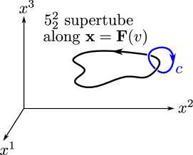
Figure -1014: The $5^{2}_{2}$ supertube along the curve ${\bf x}={\bf F}(v)$, and curve $c$ linked with it.

Eq. (5.50) means that, as we go once along $c$, $\gamma$ undergoes an additive shift,

$$\gamma\to\gamma+{4\pi nQ_{1}\over L}.$$ (5.52)

As is clear from the $x^{8},x^{9}$ part of the metric (5.46), this means that, as we travel along $c$, the radii of the internal torus $T_{89}^{2}$ do not come back to the original value. This is exactly what we observed in the straight $5^{2}_{2}$ solution (4.6). Of course, this solution is more complicated with non-vanishing RR potentials $C^{(3)},C^{(5)}$ because $5^{2}_{2}$ also carries D4 charges dissolved in its worldvolume. The $T$-duality monodromy acts on these RR fields as well.

If we move around in the spacetime without going through the curve, then $\gamma,\beta_{I}$ are single-valued and we do not see the non-geometric structure. Also, as is clear from the definition (5.40), the harmonic functions behave as $f_{I}\to 1,A\to 0$ as $|{\bf x}|\to\infty$. Namely, the spacetime is asymptotically flat. Therefore, this solution (5.46) has all the advertised features; it describes a puffed-up configuration of D4-branes with non-geometric exotic dipole charge which, being along a closed curve, does not destroy the asymptotic structure of spacetime.

The solution (5.46) has non-vanishing RR fields $C^{(3)},C^{(5)}$. Let us check that it has the expected charges. As we discussed in section 3.2 and Appendix D, there are multiple notions of charge and we must use Page charge when we want to discuss charge conservation. First, let us compute the D4 charges that we started with in the polarization process (5.4). If $S^{2}$ is a 2-sphere that encloses the entire curve in ${\mathbb{R}}^{3}$, the D4(4589) Page charge is measured by

$$Q_{\rm D4(4589)}^{\text{Page}}=\int_{S^{2}\times T^{2}_{67}}(G^{(4)}-B^{(2)}\wedge G^{(2)})=\int_{S^{2}\times T^{2}_{67}}dC^{(3)}=\int_{S^{2}}d(\gamma f_{1}^{-1}A+\beta_{2}).$$ (5.53)

Actually, for D4, Page charge or brane source charge does not make a difference because $G^{(2)}=0$. The first term in the last expression of (5.53) vanishes, since $S^{2}$ encloses the entire curve without going through it and therefore $\gamma,f_{1},A$ are all single-valued. The second term gives $Q_{2}$ by (5.51). One can similarly compute the D4(6789) charge to obtain $Q_{1}$. So, the D4 charges are given by $Q_{I}$, as expected.

Because $C^{(5)}$ is non-vanishing, one might think that this solution (5.46) carries non-vanishing D2 charges as well. However, if we look at D2 Page charges, we can show that they vanish as they should. For example, D2(45) Page charge is

$$Q_{\rm D2(45)}^{\text{Page}} =\int_{S^{2}\times T^{2}_{6789}}(G_{6}-B_{2}\wedge G_{4})=\int_{S^{2}\times T^{2}_{6789}}d(C_{5}-B_{2}\wedge C_{3})$$

$$=\int_{S^{2}\times T^{2}_{6789}}d(-f_{1}^{-1}A\wedge dx^{6}\dots dx^{9})=\int_{S^{2}}d(-f_{1}^{-1}A)=0,$$ (5.54)

because $f_{1},A$ are single valued on $S^{2}$ enclosing the entire curve. Therefore, there is no D2 charge, as expected. One can similarly see that the only monopole charges that the solution (5.46) carries are the D4-brane charges on the left of (5.4).

It is instructive to see what happens to these charges if we “go through” the curve. As discussed in section 3.2.2, this process corresponds to $U$-dualizing the notion of charge according to the $U$-duality monodromy of the exotic brane. In this process, the quantities $\gamma,\beta_{I}$ undergo additive shifts as described by (5.50), (5.51). However, we can see that D4 and D2 charges computed in (5.53) and (5.54) remain unchanged, because $\gamma,f_{1,2},A$ are still single-valued on $S^{2}$ and because (5.51) is still true. This is understood in the language we used in section 3.2 as follows. If we compactify the 10D theory on $T^{2}_{89}$ to 8D, we have $T$-duality group $SO(2,2,{\mathbb{Z}})=SL(2,{\mathbb{Z}})_{\tau}\times SL(2,{\mathbb{Z}})_{\rho}$, with moduli $\tau,\rho$ defined in (3.17) transforming in the respective $SL(2,{\mathbb{Z}})$ factors. The $5^{2}_{2}$-brane has the $T$-duality monodromy (4.15) acting on $\rho$. In 8D, D2-branes not wrapping 89 and D4-branes wrapping 89 both become 2-branes, and the 10D RR potentials $C_{\mu\nu\rho}$ and $C_{89\mu\nu\rho}$ ($\mu,\nu,\rho=0,\dots,7$) that they couple to, respectively, reduce to 8D 3-forms ${\cal C}_{\alpha\,\mu\nu\rho}$ $(\alpha=1,2)$ which transform covariantly under $SL(2,{\mathbb{Z}})_{\rho}$ as a doublet. The precise relation is [64]

$${\cal C}_{1,\mu\nu\rho}=C_{\mu\nu\rho},\qquad{\cal C}_{2,\mu\nu\rho}=C_{89\mu\nu\rho}-B_{89}C_{\mu\nu\rho}.$$ (5.55)

Just as we discussed in section 3.2, this means that ${\cal C}_{\alpha\,\mu\nu\rho}$ couple to

$${\cal Q}^{\alpha=1}=Q^{\text{D2,bs}}+B_{89}Q^{\text{D4,bs}},\qquad{\cal Q}^{\alpha=2}=Q^{\text{D4,bs}},$$ (5.56)

where $Q^{\text{D2,bs}}$ and $Q^{\text{D4,bs}}$ mean the brane source charge for D2($ij$) and D4($ij89$), respectively, with $i,j=1,\dots,7$. The covariant charges ${\cal Q}^{\alpha}$ are nothing but Page charges. Under the $SL(2,{\mathbb{Z}})_{\rho}$ duality monodromy around the $5^{2}_{2}$ given in (4.15), ${\cal Q}^{\alpha}$ transform as

$$\begin{pmatrix}{\cal Q}^{1}\\ {\cal Q}^{2}\end{pmatrix}\to\begin{pmatrix}{\cal Q}^{\prime 1}\\ {\cal Q}^{\prime 2}\end{pmatrix}=\begin{pmatrix}1&0\\ -2\pi\sigma&1\end{pmatrix}\begin{pmatrix}{\cal Q}^{1}\\ {\cal Q}^{2}\end{pmatrix}=\begin{pmatrix}{\cal Q}^{1}\\ -2\pi\sigma{\cal Q}^{1}+{\cal Q}^{2}\end{pmatrix}.$$ (5.57)

Because we originally had non-vanishing D4 charges but vanishing D2 charges, ${\cal Q}^{1}=0$ and ${\cal Q}^{2}\neq 0$. So, even after the duality transformation (5.57), we have ${\cal Q}^{\prime 1}=0,{\cal Q}^{\prime 2}={\cal Q}^{2}$. Namely, D2 and D4 Page charges remain unchanged even if we go through the $5^{2}_{2}$ ring.

Because $S^{1}\times T^{5}$ is compact, the solution (5.46) can be thought of as a solution of 4D supergravity, where D4-branes are point particles which have puffed up into a one-dimensional object, $5^{2}_{2}$. The 4D metric in the Einstein frame is

$$ds_{4}^{2} =-{1\over\sqrt{f_{1}f_{2}}}\widetilde{dt}^{2}+\sqrt{f_{1}f_{2}\,}\,dx_{123}^{2}.$$ (5.58)

The 4D Einstein metric is single-valued. In the 4D viewpoint, the monodromy of the $5^{2}_{2}$-brane appears as the monodromy of scalar moduli.

5.3 Non-geometric microstates

The 2-charge system, which is nothing but the system of two stacks of branes that appear on the left side of the puffing-up relation (1.1), (5.1)–(5.4), is known to have large microscopic degeneracy. Using weak coupling descriptions, the microscopic entropy of the system can be computed as

$$S_{\text{micro}}=2\sqrt{2}\pi\sqrt{N_{1}N_{2}},$$ (5.59)

where $N_{1},N_{2}$ are the numbers of the two branes, in the large $N_{1,2}$ limit. The strong coupling, i.e. gravity, description of the system is given by backreacted solutions of supergravity that represent the right hand side of the puffing-up relation (1.1), (5.1)–(5.4). In different duality frames, the supergravity solutions come in different guises. In particular, in the D1-D5 duality frame (5.2), the puffed-up supergravity solutions, the so-called Lunin–Mathur geometries, are configurations of Kaluza–Klein monopole with flux and are completely regular [84, 85]. By quantizing these solutions, one can reproduce the correct order of the microscopic entropy (5.59) [95]. Therefore, the Lunin–Mathur geometries give a genuine description of the microstates in supergravity, and are now called microstate geometries or geometric microstates.

In the D4-D4 system (5.4), on the other hand, we have shown that the puffed-up configurations are non-geometric solutions (5.46). They are parametrized by the profile function ${\bf F}(v)$ just as the Lunin–Mathur geometries are, and represent string theory configurations produced by back-reaction of the $5^{2}_{2}$-brane. Therefore, they are on complete equal footing with the Lunin–Mathur geometries and can accordingly equally well be viewed as a strongly-coupled description of the microstates. Namely, they are non-geometric microstates or microstate non-geometries. Note that $5^{2}_{2}$ has tension $\sim g_{s}^{-2}$, just like KKM, unlike other exotic branes with tension $\sim g_{s}^{-3}$ which makes a gravity description more questionable. Although the $5^{2}_{2}$ has singularity at the core, it must be regarded as an acceptable singularity in string theory, as the singularities of D-branes are. It is nothing more than an accident that the microstates are regular in the D1-D5 frame.

In [96], Sen claimed that, in a fixed duality frame, in the classical limit (i.e., $g_{s}\to 0$ with fixed ${\alpha^{\prime}}$), only either one of the following two possibilities must be true: (a) there only exists a small black hole solution representing the whole ensemble, or (b) there are regular gravity solutions representing individual microstates. Whether this claim is true or not remains highly controversial at the time of writing [97]. Note however that, according to Sen, the D4-D4 system is a duality frame in which there is no small black hole solution. In [96], based on a scaling argument, he argued that in the D1-D5 system there should be no classical small black hole solution. Since the D1-D5 system is related to the D4-D4 system by $T$-duality, which is perturbative and does not modify the classical limit, there must be no small black hole solution in the latter frame either. Therefore, if the claim of [96] is true, the D4-D4 system belongs to case (b) and there should be gravity microstates. The fact that we found the non-geometric microstates (5.46) seems to be in accord with this claim. However, note that Ref. [96] actually makes a stronger claim that there the gravity solution in case (b) must be smooth. The fact the metric of (5.46) is not smooth, may mean that the claim of Ref. [96] must be reconsidered in the case of non-geometric solutions; the non-geometric microstates (5.46) offer an important touchstone for the validity of the claim of [96].

5.4 Circular case

When the profile function represents a circular ring, the D4+D4$\to 5^{2}_{2}$ supertube solution (5.46) can be written down more explicitly. Let us take the profile to be

$$F_{1}(v)+iF_{2}(v)=Re^{i\omega v},\qquad F_{3}(v)=0,\qquad\omega={2\pi n\over L},$$ (5.60)

where $n\in{\mathbb{Z}}$ corresponds to the number of times the $5^{2}_{2}$ worldvolume winds around the circle of radius $R$. Let us introduce the $(y,\psi,x)$ coordinate system,

$$dx_{123}^{2} =(dx^{1})^{2}+(dx^{2})^{2}+(dx^{3})^{2}={R^{2}\over(x-y)^{2}}\left[{dy^{2}\over y^{2}-1}+(y^{2}-1)d\psi^{2}+{dx^{2}\over 1-x^{2}}\right],$$ (5.61)

$$-\infty<y\leq-1,\qquad 0\leq\psi<2\pi,\qquad-1\leq x\leq 1,$$ (5.62)

which is a 3D version of the coordinate system used for black rings [87]. $y$ is roughly a radial coordinate which goes to $-\infty$ near the ring and $-1$ near infinity (and on the axis of the ring; see Figure 1 of [98]). $x$ is an angular variable around the ring while $\psi$ is an angular variable along the ring. The explicit relations between $(x^{1},x^{2},x^{3})$ and $(y,\psi,x)$ are

$$x^{1} ={\sqrt{y^{2}-1}\over x-y}R\cos\psi,\qquad x^{2}={\sqrt{y^{2}-1}\over x-y}R\sin\psi,\qquad x^{3}=\pm{\sqrt{1-x^{2}}\over x-y}R.$$ (5.63)

As the $\pm$ sign in (5.63) indicates, we need two patches of $(y,\psi,x)$ spaces to cover ${\mathbb{R}}^{3}$. Or, we can use the $(y,\psi,\phi)$ coordinates with

$$x^{1} ={\sqrt{y^{2}-1}\over\cos\phi-y}R\cos\psi,\qquad x^{2}={\sqrt{y^{2}-1}\over\cos\phi-y}R\sin\psi,\qquad x^{3}={\sin\phi\over\cos\phi-y}R.$$ (5.64)

and

$$x=\cos\phi,\qquad 0\leq\phi\leq 2\pi.$$ (5.65)

With this range (5.65), the $(y,\psi,\phi)$ coordinates cover the entire ${\mathbb{R}}^{3}$. The inverse relation of (5.63) is

$$x=-{{\bf x}^{2}-R^{2}\over\Sigma},\qquad y=-{{\bf x}^{2}+R^{2}\over\Sigma},\qquad\Sigma^{2}=({\bf x}^{2}+R^{2})^{2}-4R^{2}x_{3}^{2}.$$ (5.66)

In this $(y,\psi,x)$ coordinate system, the functions $f_{I},A$ can be computed explicitly as

$$\begin{split}f_{I}&=1+{Q_{I}\over R}\sqrt{x-y\over-2y}\,\,_{2}F_{1}\!\left({1\over 4},{3\over 4};1;\zeta^{2}\right)=1+{2Q_{I}\over\pi R}\sqrt{{x-y\over-2y}}\,{{\bf K}({2\zeta\over\zeta-1})\over\sqrt{1-\zeta}},\\ A&=-{qR\over 2}{y^{2}-1\over(x-y)^{1/2}(-2y)^{3/2}}\,\,_{2}F_{1}\!\left({3\over 4},{5\over 4};2;\zeta^{2}\right)d\psi\\ &=-{qR\over 8}\zeta^{2}\sqrt{-2y\over x-y}\,\,_{2}F_{1}\!\left({3\over 4},{5\over 4};2;\zeta^{2}\right)d\psi,\end{split}$$ (5.67)

where $I=1,2$; ${}_{2}F_{1}(\alpha,\beta;\gamma;z)$ is the hypergeometric function and

$$Q_{2}=Q_{1}R^{2}\omega^{2},\qquad q\equiv Q_{1}\omega={2\pi nQ_{1}\over L},\qquad\zeta\equiv\sqrt{1-{1\over y^{2}}}.$$ (5.68)

Furthermore, the equations (5.44) can be solved to give

$$\gamma =-{q\sqrt{u+1}\over 4\sqrt{2}\,u^{3/2}}\biggl{\{}(1-u)\,{\bf F}\Bigl{(}{\phi\over 2}\Big{|}{2\over u+1}\Bigr{)}\,{}_{2}F_{1}\!\left({3\over 4},{5\over 4};2;\zeta^{2}\right)$$

$$\qquad\qquad+u\,{\bf E}\Bigl{(}{\phi\over 2}\Big{|}{2\over u+1}\Bigr{)}\left[3\,{}_{2}F_{1}\!\left({3\over 4},{1\over 4};2;\zeta^{2}\right)+\,{}_{2}F_{1}\!\left({3\over 4},{5\over 4};2;\zeta^{2}\right)\right]\biggr{\}}$$ (5.69)

$$=-{q\cosh{\nu\over 2}\over 4\cosh^{3/2}\nu}\biggl{\{}(1-u)\,{\bf F}\Bigl{(}{\phi\over 2}\Big{|}{1\over\sinh^{2}{\nu\over 2}}\Bigr{)}\,{}_{2}F_{1}\!\left({3\over 4},{5\over 4};2;\tanh^{2}\nu\right)$$

$$\qquad\qquad+u\,{\bf E}\Bigl{(}{\phi\over 2}\Big{|}{1\over\sinh^{2}{\nu\over 2}}\Bigr{)}\left[3\,{}_{2}F_{1}\!\left({3\over 4},{1\over 4};2;\tanh^{2}\nu\right)+\,{}_{2}F_{1}\!\left({3\over 4},{5\over 4};2;\tanh^{2}\nu\right)\right]\biggr{\}},$$ (5.70)

$$(\beta_{I})_{u} =(\beta_{I})_{\phi}=0,$$ (5.71)

$$(\beta_{I})_{\psi} ={Q_{I}\over\pi\cosh{\nu\over 2}}\biggl{\{}-e^{\nu/2}\,{\bf E}(2e^{-\nu}\sinh\nu)\,{\bf F}\Bigl{(}{\phi\over 2}\Big{|}{1\over\cosh^{2}{\nu\over 2}}\Bigr{)}$$

$$\qquad+e^{-\nu/2}{\bf K}(2e^{-\nu}\sinh\nu)\Bigl{[}-(\cosh\nu+1)\,{\bf E}\Bigl{(}{\phi\over 2}\Big{|}{1\over\cosh^{2}{\nu\over 2}}\Bigr{)}+\cosh\nu\,\,{\bf F}\Bigl{(}{\phi\over 2}\Big{|}{1\over\cosh^{2}{\nu\over 2}}\Bigr{)}\Bigr{]}\biggr{\}}$$

$$\quad+{\sqrt{2}\,Q_{I}\,e^{-\nu/2}\sin\phi\over\pi\sqrt{\cosh\nu+\cos\phi}}{\bf K}(2e^{-\nu}\sinh\nu)$$ (5.72)

where

$$u=-y=\cosh\nu,\qquad\zeta=\sqrt{1-u^{-2}}=\tanh\nu.$$ (5.73)

In the above formulae, ${\bf F}(z|m)$ and ${\bf E}(z|m)$ are the elliptic integral of the first and second kind, respectively, and ${\bf K}(m)$ and ${\bf E}(m)$ are the complete elliptic integral of the first and second kind, respectively, defined by

$${\bf E}(z|m) =\int_{0}^{z}{dt\over\sqrt{1-m\sin^{2}t}},\qquad{\bf F}(z|m)=\int_{0}^{z}\sqrt{1-m\sin^{2}t\,}\,dt$$ (5.74)

$${\bf E}(m) ={\bf E}\left({\pi\over 2}\Big{|}m\right),\qquad{\bf K}(m)={\bf F}\left({\pi\over 2}\Big{|}m\right).$$ (5.75)

By using the property of the elliptic integrals,

$${\bf E}(z+\pi|m) =2{\bf E}(m)+{\bf E}(z|m),\qquad{\bf F}(z+\pi|m)=2{\bf K}(m)+{\bf F}(z|m).$$ (5.76)

One can show that, as one goes through the ring, i.e. as $\phi\to\phi+2\pi$, the quantities $\gamma,\beta_{I}$ undergo the following additive shifts:

$$\gamma\to\gamma-2q,\qquad(\beta_{I})_{\psi}\to(\beta_{I})_{\psi}-2Q_{I}.$$ (5.77)

We can easily see that the first relation is consistent with (5.50), by looking at (5.68). On the other hand, the second relation is consistent with (5.51), as follows. As the surface $\Sigma$, take a torus that encloses the ring. Although the torus has no boundaries, make ones by cutting it along its length (namely, along $\psi$). This way, one creates two boundaries $\partial\Sigma_{1}$ and $\partial\Sigma_{2}$ such that $\partial\Sigma_{1}-\partial\Sigma_{2}=0$, both going in the $\psi$ direction; see Figure -1013.

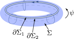
Figure -1013: 2-surface $\Sigma$ with toric topology, enclosing the circular $5^{2}_{2}$ ring. Its boundaries $\partial\Sigma_{1,2}$ are both directed along $\psi$.

Then (5.51) can be understood as saying

$$\int_{\partial\Sigma_{1}}\beta_{I}-\int_{\partial\Sigma_{2}}\beta_{I}=\int d\psi\,\Delta(\beta_{I})_{\psi}=4\pi Q_{I},$$ (5.78)

which is consistent with (5.77). In the near-ring region $y\to-\infty$ (or equivalently, $\nu\to\infty$ or $u\to\infty$), one can show

$$\gamma\approx-{q\phi\over\pi},\qquad\beta_{\psi}\approx-{Q\phi\over\pi},$$ (5.79)

from which the additive shifts (5.77) are easy to see.

5.5 Near-ring analysis

Let us study the near-ring region of the circular exotic supertube above. For a general profile, (5.42) was all we could say about the near-supertube behavior, but in this circular case we can be more explicit.

Let us define $(r,\theta,\xi)$ coordinates by

$$(x^{1})^{2}+(x^{2})^{2}=(R+r\cos\theta)^{2}-r^{2},\qquad x^{3}=r\sin\theta,\qquad\psi={\xi\over R}.$$ (5.80)

In the near-ring region $R\gg r,|x^{3}|$, these coordinates give a cylindrical coordinate system; namely, the ${\mathbb{R}}^{3}_{123}$ part of the metric is

$$ds_{123}^{2}\approx dr^{2}+r^{2}d\theta^{2}+d\xi^{2}.$$ (5.81)

In the near-ring region, the harmonic functions (5.67) reduce to

$$f_{I} \approx 1+{Q_{I}\over\sqrt{2}\,R}\,\,_{2}F_{1}\!\left({1\over 4},{3\over 4};1;1-{r^{2}\over R^{2}}\right),\quad A\approx-{qR\over 4\sqrt{2}}\,\,_{2}F_{1}\!\left({3\over 4},{5\over 4};2;1-{r^{2}\over R^{2}}\right)\,d\psi.$$ (5.82)

Expanding the hypergeometric functions, we get

$$f_{I} \approx 1+{Q_{I}\over\pi R}\log\left({8R\over r}\right),\quad A\approx-{q\over\pi}\log\left({8e^{2}R\over r}\right)\,d\xi,$$ (5.83)

from which we can explicitly see the asymptotic behavior (5.42). Also, in these coordinates,

$$\gamma =-{q\over\pi}\theta,\qquad\beta_{I}=-{Q_{I}\over\pi R}\theta\,d\xi.$$ (5.84)

In this near-ring region, the supertube can be regarded as straight. The metric becomes

$$ds^{2}\approx-\widetilde{dt}^{2}+\sqrt{f_{1}f_{2}}\,dzd{\overline{z}}+{\sqrt{f_{1}f_{2}}\over f_{1}f_{2}+\gamma^{2}}[(dx^{8})^{2}+(dx^{9})^{2}]+\dots,\qquad z=re^{i\theta}.$$ (5.85)

Let us compare this with the straight $5^{2}_{2}$ metric given by (4.52):

$$ds^{2} =-dt^{2}+{\rho_{2}e^{2\varphi_{1}}}dzd{\overline{z}}+\rho_{2}[(dx^{3})^{2}+(dx^{4})^{2}]+\dots,\qquad$$ (5.86)

By matching the corresponding metric components as

$$\sqrt{f_{1}f_{2}}\leftrightarrow{\rho_{2}e^{2\varphi_{1}}},\qquad{\sqrt{f_{1}f_{2}}\over f_{1}f_{2}+\gamma^{2}}\leftrightarrow\rho_{2},$$ (5.87)

using the asymptotic behavior (5.83), (5.84), we see that

$$\rho(z)\sim{i\over{\sqrt{Q_{1}Q_{2}}\over\pi R}\log{L\over z}},\qquad e^{\varphi(z)}\sim{\sqrt{Q_{1}Q_{2}}\over\pi R}\log{L\over z},$$ (5.88)

where $L={\cal O}(R)$. As we discussed in section 4.2, the function $e^{\varphi(z)}$ represents the freedom associated with the boundary condition at infinity, which makes the spacetime well-defined there. In the present case, we can say that the functional form of $e^{\varphi(z)}$ in (5.88) was determined so that the geometry is asymptotically flat. We see that (5.88) has the same form as for the naive, infinite stand-alone straight $5^{2}_{2}$ solution (4.61). This functional form is also the same as the F-theory case [27, 51, 60], in which one takes $e^{\varphi(z)}\propto\eta(\rho)^{-2}z^{-N/12}$ so that the transverse space has conical deficit angle $\pi N/12$. Here, $\eta(\rho)$ is the Dedekind eta function and $N$ is the number of 7-branes at $z=0$. We do not have a full understanding of why they all agree, but it is probably related to the fact that the boundary condition in all the cases is such that the energy of the codimension-2 brane does not spread all the way to infinity.

5.6 Exotic solutions versus “all supersymmetric solutions”

Based on [99], it was shown in [100] that, all supersymmetric solutions in $d=5,{\cal N}=1$ supergravity with vector multiplets in the timelike class can be written as

$$ds_{5}^{2}=-f^{2}(dt+\omega)^{2}+f^{-1}ds^{2}(M_{4}),$$ (5.89)

where $M_{4}$ is an arbitrary four-dimensional hyper-Kähler manifold and, and $f$ and $\omega$ are a scalar and a 1-form on $M_{4}$, respectively. The timelike class means that the Killing vector constructed from the bilinear of the Killing spinor is timelike.

It is interesting to see whether our exotic supertube solution fits in this framework or not. The solution (5.46) describing the exotic $\rm D4(4589)+D4(4567)\to 5^{2}_{2}(\psi 6789,45)$ supertube is not appropriate for this for the following reason. In order to put this in the framework of $d=5$ supergravity, we first lift this to $\rm M5(4589{\rm A})+M5(4567{\rm A})\to 5^{3}(\psi 6789,45{\rm A})$, where ${\rm A}$ denotes the 11th direction, and compactify it on $456789$. However, this solution belongs to the null class, not the timelike one, because the naive M5-M5 solution is in the null class and the Killing spinors of the two configurations must agree asymptotically.

So, we should go to a different duality frame where the solution is timelike and involves exotic charge. By $T$-dualizing (5.46) along $67$, we obtain $\rm D6(456789)+D2(89)\to 5^{2}_{2}(\psi 4567,89)$, which is an exotic supertube. By further lifting it to 11 dimensions, we get an exotic supertube in M-theory, $\rm KKM(456789,{\rm A})+M2(89)\to 5^{3}(\psi 4567,89{\rm A})$. This must belong to the timelike class, because the naive KKM+M2 solution does. The 11D metric and 3-form for this exotic supertube solution are

$$\begin{split}ds_{11}^{2}&=-f_{1}^{-2/3}F^{-2/3}\left[dt+f_{2}^{-1}\gamma(dx^{\rm A}+\beta_{2})-FA\right]^{2}+f_{1}^{1/3}f_{2}F^{1/3}dx_{123}^{2}\\ &\qquad+f_{1}^{1/3}f_{2}^{-1}F^{1/3}(dx^{\rm A}-f_{1}^{-1}\gamma A+\beta_{2})^{2}+f_{1}^{1/3}F^{1/3}dx_{4567}^{2}+f_{1}^{-2/3}F^{-2/3}dx_{89}^{2},\\ A_{3}&=\left[{f_{2}\widetilde{dt}+\gamma(dx^{\rm A}+\beta_{2})\over f_{1}f_{2}+\gamma^{2}}-dt\right]\wedge dx^{8}\wedge dx^{9},\end{split}$$ (5.90)

where

$$F\equiv 1+{\gamma^{2}\over f_{1}f_{2}}.$$ (5.91)

To put this in the form of $d=5$ supergravity, we compactify it on $456789$ and keep the $0123{\rm A}$ part. The 5D metric is

$$ds_{5}^{2} =-f^{2}\left[dt+f_{2}^{-1}\gamma(dx^{\rm A}+\beta_{2})-FA\right]^{2}+f^{-1}ds_{4}^{2},$$ (5.92)

where

$$ds_{4}^{2} =f_{2}^{-1}(dx^{\rm A}-f_{1}^{-1}\gamma A+\beta_{2})^{2}+f_{2}dx_{123}^{2},\qquad f=f_{1}^{-1/3}F^{-1/3}.$$ (5.93)

The metric (5.92) appears to be of the general form (5.89). However, it is easy to see that the 4D base metric (5.93) is not hyper-Kähler; the Ricci tensor does not vanish due to the $f_{1}^{-1}\gamma A$ term.

This suggests that, because exotic supertubes describe non-geometric spacetimes in which fields have non-trivial monodromies, the existing classification of “all supersymmetric solutions” does not apply to them. It would be very interesting to nail down what assumptions in the existing analysis should be relaxed and generalize the classification of supersymmetric configurations to incorporate exotic solutions.

6 Toward “truly non-geometric” configurations

One could say that the exotic solutions we have discussed so far are not truly non-geometric, in the sense that there are duality frames where they are geometric, and that the Einstein metric in the lower (non-compact) dimensions is single-valued. In this section, we discuss the existence of exotic solutions for which

• spacetime is non-geometric, i.e., the metric is multi-valued, in any duality frames,

• even the Einstein metric in the lower (non-compact) dimensions is multi-valued.

The non-geometric solutions satisfying condition (i) have been known (see, e.g., [46, 102, 103, 104]). Here we discuss it using the model related to the one in previous sections. Furthermore, using the same model, we argue for the existence of solutions satisfying the stronger condition (ii).

For this purpose, let us consider the following simple model. We compactify 10D string on $T^{2}\times T^{5}$, where the $T^{5}$ metric is flat and there is no form fields along it. So, the 10D string frame metric can be written as

$$ds_{\text{10,str}}^{2} =ds_{5}^{2}+\sum_{a=5}^{9}(dx^{a})^{2},\qquad ds_{5}^{2}=e^{2\Phi}G^{-1}ds_{\text{3,Ein}}^{2}+ds^{2}_{T^{2}},$$ (6.1)

where $\Phi$ is the 10D dilaton. Moreover, $ds_{\text{3,Ein}}^{2}$ is the Einstein metric in non-compact 3D and $ds_{T^{2}}^{2}$ is the metric on $T^{2}$, given by

$$\begin{split}ds_{\text{3,Ein}}^{2}&=g_{\mu\nu}dx^{\mu}dx^{\nu},\qquad\mu,\nu=0,1,2,\\ ds_{T^{2}}^{2}&=G_{ij}(dx^{i}+A^{i}_{\mu}dx^{\mu})(dx^{j}+A^{j}_{\nu}dx^{\nu}),\qquad G=\det G_{ij},\qquad i,j=3,4,\end{split}$$ (6.2)

where $g_{\mu\nu},G_{ij},A^{i}_{\mu}$ depend only on $x^{\mu}$. If we write the internal $T^{2}$ fields as

$$\begin{split}ds_{T^{2}}^{2}&={\rho_{2}\over\tau_{2}}|dx^{3}+\tau dx^{4}|^{2},\qquad G_{ij}={\rho_{2}\over\tau_{2}}\begin{pmatrix}1&\tau_{1}\\ \tau_{1}&|\tau|^{2}\end{pmatrix},\qquad\tau=\tau_{1}+i\tau_{2},\\ \rho&=B_{34}+iG^{1/2}=\rho_{1}+i\rho_{2},\end{split}$$ (6.3)

then the 3D action is

$$S_{3D}=\int d^{3}x\sqrt{-g}\left(R_{g}-4(\nabla\phi)^{2}-{|\nabla\tau|^{2}\over 2\tau_{2}^{2}}-{|\nabla\rho|^{2}\over 2\rho_{2}^{2}}\right),\qquad\phi\equiv\Phi-{1\over 4}\log G.$$ (6.4)

The equations of motion for $\phi$ and $\tau$ are

$$\nabla^{2}\phi=0,\qquad\qquad\nabla_{\mu}\left({\nabla^{\mu}\tau_{1}\over\tau_{2}^{2}}\right)=0,\qquad\nabla_{\mu}\left({\nabla^{\mu}\tau_{2}\over\tau_{2}^{2}}\right)+{|\nabla\tau|^{2}\over\tau_{2}^{3}}=0.$$ (6.5)

The $\rho$ equations of motion are obtained from the $\tau$ equations by setting $\tau\to\rho$. In addition, $g_{\mu\nu}$ should satisfy the 3D Einstein equation

$$\begin{split}&R_{\mu\nu}-{1\over 2}g_{\mu\nu}R=T_{\mu\nu},\\ &T_{\mu\nu}=4\Bigl{(}\partial_{\mu}\phi\partial_{\nu}\phi-{1\over 2}{g_{\mu\nu}}|\partial\phi|^{2}\Bigr{)}+{1\over 4\tau_{2}^{2}}\left(\partial_{\mu}{\overline{\tau}}\partial_{\nu}\tau+\partial_{\nu}{\overline{\tau}}\partial_{\mu}\tau-{g_{\mu\nu}}|\partial\tau|^{2}\right)+(\tau\to\rho).\end{split}$$ (6.6)

This theory describes 3D gravity coupled to two scalars $\tau,\rho$, and has duality group $SL(2,{\mathbb{Z}})\times SL(2,{\mathbb{Z}})\times{\mathbb{Z}}_{2}^{2}$. The $SL(2,{\mathbb{Z}})\times SL(2,{\mathbb{Z}})$ factor acts on $\tau,\rho$ in an obvious way. The first ${\mathbb{Z}}_{2}$ exchanges $\tau\leftrightarrow\rho$ while the second ${\mathbb{Z}}_{2}$ sends $(\tau,\rho)\to(-{\overline{\tau}},-{\overline{\rho}})$ [63]. This is the theory studied in [27] in relation to cosmic strings and in [46] further in the context of non-geometric compactifications. A particular solution of this is given by

$$ds^{2}_{\text{3,Ein}} =-dt^{2}+e^{U}dzd{\overline{z}},\qquad z=x^{1}+ix^{2},$$ (6.7)

$$\phi =0,\qquad\tau=\tau(z),\qquad\rho=\rho(z),\qquad e^{U}=\tau_{2}\rho_{2}|f(z)|^{2},$$ (6.8)

where $\tau(z),\rho(z),f(z)$ are arbitrary holomorphic functions subject to the condition that $e^{U}$ is single valued. If $\tau(z)$ has an $SL(2,{\mathbb{Z}})$ monodromy around a point on the $z$-plane, say $z=\alpha$, there is a codimension-2 brane (which we call a $\tau$-brane) at $z=\alpha$ and the internal $T^{2}$ is non-trivially fibered around it. However, the total 5D spacetime is still geometric because $T^{2}$ is glued with the same $T^{2}$ via a basis change. On the other hand, if $\rho(z)$ has an $SL(2,{\mathbb{Z}})$ monodromy around $z=\alpha$ (which we call a $\rho$-brane), this generally means that the 5D spacetime is non-geometric, because the metric components and $B$-field are mixed into each other as we go around $z=\alpha$.

Not all $\rho$-brane branes are non-geometric; the $\rho$-brane around which $\rho$ simply shifts as $\rho\to\rho+1$ is geometric. Therefore, if there is a single non-geometric $\rho$-brane, we can always do an $SL(2,{\mathbb{Z}})$ duality transformation to make it geometric. However, this is not possible if there are multiple $\rho$-branes with different monodromies at different points, because we cannot dualize all non-geometric $\rho$-branes into geometric ones at the same time. One could use the ${\mathbb{Z}}_{2}$ duality $\tau\leftrightarrow\rho$ to transform non-geometric $\rho$-branes into $\tau$-branes which are always geometric, but if there exist multiple $\tau$-branes and $\rho$-branes at the same time, such ${\mathbb{Z}}_{2}$ duality transformation cannot reduce the solution geometric. The other ${\mathbb{Z}}_{2}$ symmetry does not help either. Therefore, such solutions are concrete examples that are non-geometric in the sense of (i).

Now let us move on to the second issue (ii), whether we can have a configuration that is non-geometric even in lower dimensions. Here, we would like to use the same model (6.2) to argue that there are configurations which are (initially) asymptotically flat ${\mathbb{R}}^{1,3}$ and whose four-dimensional metric has non-trivial monodromies.

To begin with, let us take flat ${\mathbb{R}}^{1,3}\times S^{1}$ with metric

$$ds_{5}^{2} =-dt^{2}+dx^{2}+d\xi^{2}+d\eta^{2}+dy^{2},\qquad t,x,\xi,\eta\in{\mathbb{R}},\qquad y\cong y+2\pi.$$ (6.9)

This is a 4D spacetime (times a compact $S^{1}$), but let us do an angular compactification of ${\mathbb{R}}^{1,3}$ by going to polar coordinates $(r,\theta)$ for the $(\xi,\eta)$ plane as

$$\begin{split}\xi&=r\cos\theta,\quad\eta=r\sin\theta;\qquad r\geq 0,\quad\theta\cong\theta+2\pi,\\ ds_{5}^{2}&=-dt^{2}+dx^{2}+dr^{2}+r^{2}d\theta^{2}+dy^{2},\end{split}$$ (6.10)

and compactifying on the angle $\theta$. Namely, we regard $y,\theta$ as the $T^{2}$ coordinates of the 5D$\to$3D compactification (6.1), (6.2), by taking $x^{3}=y,x^{4}=\theta$. Then the “3D” fields (6.3), (6.4) are,

$$ds_{\text{3,Ein}}^{2} =r^{2}(-dt^{2}+dx^{2}+dr^{2}),\qquad\tau=\rho=ir,\qquad\phi=-{1\over 2}\log r,$$ (6.11)

where we set the 10D dilaton $\Phi=0$ so that the flat spacetime (6.9) is trivially a solution. This is a perverse way to write non-compact ${\mathbb{R}}^{1,3}$ times compact $S^{1}$ as a $T^{2}$ fibration over ${\mathbb{R}}^{1,2}$, although there is nothing wrong with it. The 4D Einstein frame metric is simply ${\mathbb{R}}^{1,3}$:

$$ds^{2}_{\text{4,Ein}} ={e^{2\phi}\over\sqrt{\tau_{2}\rho_{2}}}ds_{\text{3,Ein}}^{2}+{\sqrt{\tau_{2}\rho_{2}}\over e^{2\phi}}(dx^{4})^{2}=-dt^{2}+dx^{2}+dr^{2}+r^{2}d\theta^{2}.$$ (6.12)

In this setup, a configuration that is non-geometric in the non-compact 4D spacetime is one that has non-trivial monodromy of $\rho$ over the 3D base and asymptotes to (6.11) as $r\to\infty$. Furthermore, the fields should behave as (6.11) also as $r\to 0$, in order for the point $r=0$ to represent a smooth point in spacetime. See Figure -1012 for a schematic explanation.

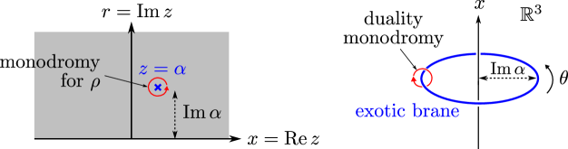
Figure -1012: A point on the upper half $z$-plane around which there is non-trivial monodromy for $\rho$ (left) corresponds to a circular exotic brane extended in the $\theta$ direction in ${\mathbb{R}}^{3}$ (right).

It is difficult to find an actual solution that satisfies the equations of motion (6.5), (6.6) and has such non-geometric monodromy for $\rho$. Here, let us content ourselves by writing down a static configuration which has such non-geometric monodromy but does not satisfy the equations of motion. One can certainly use such a configuration as an initial condition to find a time-dependent solution of the equations of motion. Therefore, the existence of such a configuration is evidence for a non-geometric solution in low dimensions.

To find such a non-geometric configuration, let us fix the 3D metric to be simply (6.11), which we write as

$$ds_{\text{3,Ein}}^{2}=(\mathop{\mathrm{Im}}\nolimits z)^{2}(-dt^{2}+dzd{\overline{z}}),\qquad z\equiv x+ir,\qquad\mathop{\mathrm{Im}}\nolimits z\geq 0.$$ (6.13)

On this fixed base metric, let us consider 3D fields $\tau(z,{\overline{z}}),\rho(z,{\overline{z}})$ which do not necessarily satisfy the equations of motion. Assume that, at $z=\alpha$ ($\mathop{\mathrm{Im}}\nolimits\alpha>0$), the field $\rho$ undergoes an $SL(2,{\mathbb{Z}})$ monodromy

$$\rho~{}\to~{}\rho^{\prime}={a\rho+b\over c\rho+d},\qquad a,b,c,d\in{\mathbb{Z}},\qquad ad-bc=1.$$ (6.14)

This corresponds to having a circular exotic brane in the spatial ${\mathbb{R}}^{3}$ at $z=\alpha$; see Figure -1012. Because $\mathop{\mathrm{Im}}\nolimits z=r=0$ is a special point (the origin of the polar coordinates), the fields $\rho,\tau$ should behave in a particular way near $r=0$ for the 5D geometry to be regular there. However, in the presence of a $\rho$-monodromy, even if we start from a metric for which $r=0$ is a regular point, after we go around the exotic brane, we may end up with a metric for which $r=0$ is singular. Because this is physically unacceptable, let us require that the 5D metric be regular even if we go around the brane and come back near $r=0$. Then, we ask what constraint this requirement imposes on the possible monodromy $M=\left(\begin{smallmatrix}a&b\\ c&d\end{smallmatrix}\right)$.

Let us assume that there is a brane at $z=\alpha$ with $\mathop{\mathrm{Im}}\nolimits z>0$, and that the behavior of $\rho$ near $r=0$ is still given by (6.11). Namely,

$$\rho_{1}={\cal O}(r),\qquad\rho_{2}=r+{\cal O}(r^{2})\qquad\qquad(r\to 0).$$ (6.15)

We take this $\rho$ because we know that this gives a regular 5D geometry. Now consider starting from the small $r$ region where (6.15) is valid, moving away from $r=0$, going around $z=\alpha$, and coming back to the small $r$ region again. After this process, the $\rho$ gets transformed into

$$\rho^{\prime}_{1} ={ac|\rho|^{2}+(ad+bc)\rho_{1}+bd\over|c\rho+d|^{2}}={bd+acr^{2}\over d^{2}+c^{2}r^{2}},$$ (6.16)

$$\rho^{\prime}_{2} ={\rho_{2}\over|c\rho+d|^{2}}={r\over d^{2}+c^{2}r^{2}}.$$ (6.17)

For simplicity, we assume that $\phi,\tau$ are unchanged and has no monodromy: $\phi=-(1/2)\log r$, $\tau^{\prime}=ir$. As $r\to 0$, we want the volume of the torus $\rho_{2}^{\prime}$ to vanish just as $\rho_{2}$ did. So, let us set $d^{2}=1$. If we require also that the $B$-field $B_{34}^{\prime}=\rho_{2}^{\prime}$ vanish at $r=0$, we need $b=0$. Then the condition $ad-bc=1$ says that

$$M =\begin{pmatrix}1&0\\ c&1\end{pmatrix},\qquad c\in{\mathbb{Z}},$$ (6.18)

where we took $d=+1$ since the overall sign of $M$ does not matter. For this monodromy matrix (6.18), the transformed $\rho$ is

$$\rho^{\prime}_{1} ={cr^{2}\over 1+c^{2}r^{2}},\qquad\rho^{\prime}_{2}={r\over 1+c^{2}r^{2}}.$$ (6.19)

The transformed 5D fields are, from (6.2),

$$ds_{5}^{\prime 2}=-dt^{2}+dx^{2}+dr^{2}+{r^{2}d\theta^{2}+dy^{2}\over 1+c^{2}r^{2}},\quad B^{\prime}_{y\theta}={acr^{2}\over 1+c^{2}r^{2}}\qquad(r\to 0).$$ (6.20)

The 4D Einstein metric is, using the middle expression in (6.12),

$$ds_{\text{4,Ein}}^{\prime 2}=\sqrt{1+c^{2}r^{2}}(-dt^{2}+dx^{2}+dr^{2})+{r^{2}\over\sqrt{1+c^{2}r^{2}}}d\theta^{2}.$$ (6.21)

This geometry is indeed regular at $r=0$, both in 4D and 5D. So, in this configuration, we started from a regular, asymptotically flat 4D geometry (times a compact $S^{1}$) and, even after going through an exotic monodromy (which mixes the internal $S^{1}$, the angular direction $\theta$, and the $B$-field through these two directions), we still have a regular geometry. Note that, the transformed Einstein metric (6.21) is not just different from the original form (6.12) but has an asymptotics totally different from the one we started from. By going through an exotic brane, one ends up with a totally different universe!

We still have to find an explicit field configuration $\rho(z,{\overline{z}})$ which does have the monodromy (6.18) at $z=\alpha$. A naive first try is

$$\rho(z,{\overline{z}}) ={1\over{2\over z-{\overline{z}}}+{c\over 2\pi i}\ln(z-\alpha)},$$ (6.22)

which indeed behaves near $r=\mathop{\mathrm{Im}}\nolimits z\to 0$ as

$$\rho(z,{\overline{z}}) \sim ir\qquad(r\sim 0)$$ (6.23)

and has the desired monodromy around $z=\alpha$:

$$\rho \to\rho^{\prime}={\rho\over 1+c\rho}.$$ (6.24)

However, at large $r$, this $\rho$ goes like

$$\rho(z,{\overline{z}}) \sim{1\over{c\over 2\pi i}\ln(z-\alpha)}\qquad(r\to\infty)$$ (6.25)

instead of $\rho(z,{\overline{z}})\to ir$, which is necessary to have the correct original asymptotics (even before going through the exotic brane). So, (6.22) is too simple.

This problem can be circumvented by considering a configuration with branes and anti-branes at the same time. For example, take

$$\rho(z,{\overline{z}}) ={1\over{2\over z-{\overline{z}}}+{c\over 2\pi i}\ln{(z-\alpha)(z-\beta)\over(z-\gamma)(z-\delta)}},\qquad\alpha+\beta-\gamma-\delta=0.$$ (6.26)

Namely, we placed branes at $z=\alpha,\gamma$ and anti-branes at $z=\beta,\delta$. As long as we keep away from the centers, this has the desired asymptotics,

$$\rho(z,{\overline{z}})=\begin{cases}ir+{\cal O}(1)&\qquad r\to\infty,\\ ir+{\cal O}(r^{2})&\qquad r\to 0,\end{cases}$$ (6.27)

so that the original geometry is regular at $r=0$ and is asymptotically flat ${\mathbb{R}}^{1,3}\times S^{1}$, as desired.

If we go around one of the branes (but not all of them), $\rho$ changes into

$$\rho\to\rho^{\prime} ={1\over{2\over z-{\overline{z}}}+c+{c\over 2\pi i}\ln{(z-\alpha)(z-\beta)\over(z-\gamma)(z-\delta)}}.$$ (6.28)

The $r\to 0,\infty$ behavior is now

$$\rho(z,{\overline{z}})=\begin{cases}{1\over c}+{i\over c^{2}r}+{\cal O}(r^{-2})&\qquad r\to\infty,\\[4.30554pt] ir+{\cal O}(r^{2})&\qquad r\to 0.\end{cases}$$ (6.29)

This is exactly the same as (6.20), as it should be.

Note that, the position of the branes and anti-branes, $\alpha,\beta,\gamma$ and $\delta$, does not have to be in the $r>0$ region. So, for example, we can have only one real brane at $z=\alpha$ with $\mathop{\mathrm{Im}}\nolimits\alpha>0$, and all others can be some kind of “image” branes with $\mathop{\mathrm{Im}}\nolimits\beta,\mathop{\mathrm{Im}}\nolimits\gamma,\mathop{\mathrm{Im}}\nolimits\delta<0$ which are necessary to make the asymptotics right. This is just like the method of image charges in electromagnetism.

So, there certainly is a configuration of exotic branes leading to non-geometric structure in the Einstein metric for the lower, non-compact dimensions. We found a configuration of circular exotic branes (with anti-branes and/or image charges) in asymptotically flat ${\mathbb{R}}^{3,1}\times S^{1}$. As long as we keep away from the exotic brane, the spacetime remains asymptotically flat but, if we go through the brane, we go to a different spacetime with different asymptotics. This configuration does not satisfy the equation of motion and therefore is not an actual solution of the theory. However, it certainly gives evidence for the existence of spacetimes with property (ii) at the beginning of this section. It would be very interesting to find an actual solution of string theory with property (ii).

7 Exotic branes and black holes

The supertube effect is a phenomenon in which some particular combination of branes, when put together, produces a new type of brane. One notable situation in string theory where multiple branes are put together is the black hole. In this section, we discuss the supertube effect in the context of black holes. In particular, we argue that, via a multi-stage supertube effect, or “double bubbling”, exotic branes play an important role in black hole physics.

So far we discussed the supertube effect in which two types of brane are put together, producing one new type of brane. However, we can put together three types of brane. As an example, take the 3-charge M2 system [89] which is a well studied configuration in the context of 5D black hole microstate counting [105]. In this case, the puffing up is known to occur as

$$\begin{array}[]{l}\rm M2(56)\\ \rm M2(78)\\ \rm M2(9{\rm A})\end{array}\to\begin{array}[]{l}\rm M5(\psi 789{\rm A})\\ \rm M5(\psi 569{\rm A})\\ \rm M5(\psi 5678)\end{array},$$ (7.7)

where “${\rm A}$” denotes the $x^{10}$ direction. Namely, the puffing up occurs pairwise, producing three daughter branes which extend along an arbitrary curve parametrized by $\psi$ in ${\mathbb{R}}^{4}_{1234}$. The black ring solution [98, 88, 89] is the manifestation of this puffing up actually occurring.

Actually, the daughter charges on the right of (7.7) include combinations of charges which can pairwise puff up again, in principle. Such a second puffing-up would be:

$$\begin{array}[]{l}\rm M2(56)\\ \rm M2(78)\\ \rm M2(9{\rm A})\end{array}\to\begin{array}[]{l}\rm M5(\psi 789{\rm A})\\ \rm M5(\psi 569{\rm A})\\ \rm M5(\psi 5678)\end{array}\to\begin{array}[]{l}\rm 5^{3}(\phi 789{\rm A},\psi 56)\\ \rm 5^{3}(\phi 569{\rm A},\psi 78)\\ \rm 5^{3}(\phi 5678,\psi 9{\rm A})\end{array}\to\cdots$$ (7.17)

Namely, the system can polarize into exotic $5^{3}$ branes extended along a surface parametrized by $\psi,\phi$ in ${\mathbb{R}}^{4}_{1234}$. This is the multi-stage supertube effect whose possibility was first pointed out by the current authors in [7]. In [31], a supersymmetry argument was given in strong support for such multi-stage supertube effect being indeed possible. The conjectured supersymmetric object along an arbitrary surface was dubbed superstratum in [31].

Furthermore, as the dots in (7.17) indicate, the “granddaughter” $5^{3}$-branes again form a combination that can combine to produce still more charges. Therefore, it appears that this puffing-up process can in principle continue indefinitely, producing all kinds of exotic charges appearing in Table 2. If this is the case, then the final state will be a complicated configuration of exotic superstrata. Conversely, it is also possible that this process happens only a finite number of times for some dynamical reason. For example, whether supertubes provide a good (i.e. weakly coupled) description of bound states depends on the string coupling and on the other parameters of the theory, so presumably a similar statement is valid for more complicated types of transitions. Either way, it would be very interesting to investigate such processes can indeed happen or not.

Another well-known example is the D0-D4-D4-D4 system, which has been intensively studied in the context of 4D black hole microstate counting [90], and involves four stacks of branes: D0, D4(6789), D4(4589), D4(4567). If we bring these four stacks together, each pair is expected to puff up into a new brane stack:

$${\rm D0}~{}~{}\begin{array}[]{l}\rm D4(6789)\\ \rm D4(4589)\\ \rm D4(4567)\end{array}~{}~{}\to~{}~{}\begin{array}[]{l}\rm NS5(6789\psi)\\ \rm NS5(4589\psi)\\ \rm NS5(4567\psi)\end{array}\begin{array}[]{l}\rm 5^{2}_{2}(6789,45\psi)\\ \rm 5^{2}_{2}(4589,67\psi)\\ \rm 5^{2}_{2}(4567,89\psi)\end{array}$$ (7.27)

Interestingly, exotic branes make their appearance even at the first stage of puffing up in this system. The $\rm D4+D4\to 5^{2}_{2}$ supertube we studied in section 5 in detail is only a part of this process. Therefore, a gravity description of black hole physics in this frame inevitably involves exotic branes. It would be interesting to find a solution corresponding to the right hand side of (7.27). Also in this case, the daughter branes on the right form a combination that can combine and produce new branes. Again, the final state would be exotic superstrata along complicated surfaces.

In the 2-charge system [84], the microscopic entropy comes from the Higgs branch of the worldvolume theory associated with the intersection of two stacks of branes. In gravity, the same entropy is explained by the degrees of freedom coming from the fluctuations of the one-dimensional geometric object which is the result of puffing up the intersection [95]. In the 3-charge system, the triple intersection of three stacks of branes leads to a more complicated Higgs branch and larger microscopic entropy. It is conceivable that the fluctuations of the above 2-dimensional exotic superstratum that naturally appears, with its larger number of degrees of freedom, account for the entropy of the 3-charge system. It would hence be very interesting to construct non-geometric solutions involving such exotic charges to see if they can really reproduce the expected entropy. The fact that the 3-charge supergravity microstates constructed thus far (see e.g. [106, 107]) do not seem enough to account for the entropy of the 3-charge black hole [107] may be related to the non-geometric nature of exotic branes that have been overlooked.

In the explicitly known examples of microstate geometries for large supersymmetric black holes (see e.g. [106, 108, 107]) such exotic charges do not appear, and it has been argued that purely geometric microstates alone cannot account for their entropy [107]. It would be very interesting to study and classify microstate geometries involving exotic dipole charges, to see whether they can provide the missing microstate geometries, and study their implications for black hole physics and the fuzzball conjecture [32].

The multi-stage supertube effect, if it does occur, is special to systems with 3 or more branes. Because the daughter charge of a supertube effect are not such that can combine with the parent charges to produce a new charge, one needs more than two daughter charges to produce a granddaughter. This requires more than three parent charges to begin with. It is a curious coincidence that one needs at least three stacks of branes to have a black hole with finite horizon in string theory.

Also, it makes sense to construct black hole microstates using codimension-2 objects, because they cannot be “fattened”. Namely, supergravity solutions representing branes with codimension three or larger can always be made non-extremal with a finite horizon, but there is no non-extremal supergravity solution for codimension-2 branes. This is easy to see. The metric produced by black D$p$-branes is [111], by setting $q\equiv 7-p$,

$$ds_{\text{10,str}}^{2} =H^{-1/2}(-Kdt^{2}+dx_{1}^{2}+\dots+dx_{p}^{2})+H^{1/2}(K^{-1}dr^{2}+r^{2}d\Omega_{q+1}^{2}),$$

$$H =h_{0}+\zeta\left({r_{0}\over r}\right)^{q},\qquad K=1-\left({r_{H}\over r}\right)^{q},$$ (7.28)

$$r_{0}^{q} =c_{q}g_{s}Nl_{s}^{q},\quad c_{q}=(2\sqrt{\pi})^{q-2}\,\Gamma\!\left(\frac{q}{2}\right),\quad\zeta=\sqrt{1+\left[{1\over 2}\left({r_{H}\over r_{0}}\right)^{q}\right]^{2}}-{1\over 2}\left({r_{H}\over r_{0}}\right)^{q},$$

where $N$ is the number of D$p$-branes, and $r_{H}$ is the position of the horizon. The constant $h_{0}$ can be set to one by rescaling of coordinates, but we leave it arbitrary. We only displayed the metric, but other fields are also excited. In the extremal limit, $r_{H}\to 0,\zeta\to 1,K\to 1$. If we further take the limit $p\to 7$ ($q\to 0$),

$$H=h_{0}+c_{q}g_{s}N\left({l_{s}\over r}\right)^{q}~{}\xrightarrow{q\to 0}~{}{g_{s}N\over 2\pi q}+h_{0}+{g_{s}N\over 2\pi}\log{l_{s}\over r}+{\cal O}(q).$$ (7.29)

Although the first term on the right is divergent as $q\to 0$, it can be made finite by absorbing it into $h_{0}$. This way we can obtain the metric for extremal D7-branes. Let us ask if we can turn on non-extremality $r_{H}>0$ keeping fields finite. If we set $r_{H}^{q}=a(q)\rho_{H}^{q}$, where $a(q)$ is some function of $q$,

$$K\xrightarrow{q\to 0}1-a(q)-a(q)q\log\left({\rho_{H}\over r}\right).$$ (7.30)

In order to have a horizon, we need to keep the log so that $K=0$ has a solution. This means that we need to take $a(q)\sim q^{-1}$ but this will make $K$ diverge as $q\to 0$. Therefore, there does not exist a non-extremal D7-brane solution. One may wonder if one can find codimension-2 black holes in the blackfold approach [112, 113]. However, this approach is applicable only when there are two widely separated scales in the problem (thickness and curvature of the horizon), which is not the case for codimension-2 objects. Therefore, it is also consistent with non-existence of codimension-2 black holes. The fact that there is no “fat” codimension-2 object is good because, if a microstate solution could be made non-extremal, or fattened, then we would need some other objects to explain its Bekenstein–Hawking entropy!

Although generic superstrata are expected to be exotic and thus non-geometric, there can be special cases in which superstrata are completely geometric. Such geometric superstrata might not be sufficient for the ultimate goal of reproducing black hole entropy, they are very interesting in their own right and should also help us understand non-geometric superstrata. Geometric superstrata should be describable within usual supergravity. For recent progress toward constructing such geometric superstrata in the context of 6D supergravity, see [114, 115].

In Eq. (5.8), we showed that the BPS bound state of two kinds of brane with mass $g_{s}^{-a}$ and $g_{s}^{-b}$ is a supertube, which is made of a brane with tension $T\sim g_{s}^{-(a+b)}$ and which is spreading over distance $R\sim g_{s}^{(a+b)/2}$. Then it is tempting to conjecture that the BPS bound state of three kinds of brane with mass $g_{s}^{-a},g_{s}^{-b},g_{s}^{-c}$ is a superstratum with tension $T\sim g_{s}^{-(a+b+c)}$, typically spreading over distance $R\sim g_{s}^{(a+b+c)/2}$, and that the bound state of four kinds of brane with mass $g_{s}^{-a},g_{s}^{-b},g_{s}^{-c},g_{s}^{-d}$ is a superstratum with tension $g_{s}^{-(a+b+c+d)}$ spreading over distance $R\sim g_{s}^{(a+b+c+d)/2}$. Based on this, we can make an interesting observation, as follows. Let us further assume that non-supersymmetric black holes are also made of polarized branes spreading over distance $R\sim g_{s}^{(a+b+c)/2}$ or $R\sim g_{s}^{(a+b+c+d)/2}$, and require that this $R$ reproduce the horizon radius of the Schwarzschild black hole in $D$ dimensions,

$$r_{H}\sim(G_{D})^{{1\over D-3}}\sim(g_{s})^{2\over D-3},$$ (7.31)

where $G_{D}\sim g_{s}^{2}$ is the $D$-dimensional Newton constant. The relation (7.31) gives, for example,

$$D=6:~{}r_{H}\sim g_{s}^{2/3},\qquad D=5:~{}r_{H}\sim g_{s},\qquad D=4:~{}r_{H}\sim g_{s}^{2},$$ (7.32)

which is to be equal to $R\sim g_{s}^{(a+b+c)/2}$ or $R\sim g_{s}^{(a+b+c+d)/2}$. Because the mass of branes always come in integral powers of $1/g_{s}$, it is impossible to have $R\sim r_{H}$ in $D=6$. On the other hand, for $D=4,5$, it is possible to have brane charges satisfying $R\sim r_{H}$. For example,

D1-D5-P system in $$D=5 : \quad(a,b,c) =(1,1,0), T \sim g_{s}^{-2}, R\sim g_{s},$$ (7.33)

D0-D4-D4-D4 system in $$D=4 : \quad(a,b,c,d) =(1,1,1,1), T \sim g_{s}^{-4}, R\sim g_{s}^{2}.$$ (7.34)

The first line (7.33) suggests that the microstates of the D1-D5-P black hole are described by polarized branes with tension $T\sim g_{s}^{-2}$. In [114, 115], it was argued that the microstates of the supersymmetric D1-D5-P black hole include geometric superstrata made of wiggly D1-D5 branes puffed up into wiggly KK monopoles, which have tension $\sim g_{s}^{-2}$. The above seems to give support to such geometric superstrata actually being the typical microstates of this system. On the other hand, (7.34) suggests that the microstates of the 4D black hole involves very exotic objects with tension $g_{s}^{-4}$ and its description in terms of (multi-valued) metric in 10D is physically more questionable, if not totally nonsensical. One either has to go to 11D or use the metric only as a qualitative guide. The above discussion is very crude and not intended to be a rigorous argument, equating the size of the supersymmetric superstrata and the horizon radius of the Schwarzschild black hole. However, we deem this as an interesting and suggestive observation.

If a black hole microstate is made of some kind of supertube/superstratum of exotic branes, one can imagine an object freely falling into it. The exotic supertube has some duality monodromy around it. Therefore, when the object goes into the microstate, it is expected to generically go through the exotic superstratum and undergo a duality transformation. After exploring the complicated structure of the superstratum, the object will eventually come back out (after a long time which goes to infinity in the classical limit $G_{N}\to 0$). For an observer sitting at infinity, it appears that the object is no longer the same entity but has turned into a $U$-dual version. On the other hand, from the point of view of the object, it appears that it has returned to a different world—the $U$-dual version of the original world it started from. Of course, these two pictures are consistent because they are only different (dual) descriptions of the same physics. This is reminiscent of the still controversial black hole complementarity [116, 117] which claims that the two pictures of an object fallen into a black hole, in one of which the object gets returned in the form of Hawking radiation and in the other of which the object crosses the horizon unscathed, are two different descriptions of the same physics. Here we only point out this amusing similarity and leave further investigations for future research.

In this paper, we have been arguing that exotic branes are generic objects, and hence that, if we consider generic situations in string theory, they will inevitably show up. If we think this way, it is natural that black holes must involve exotic branes. Very near the horizon of a black hole, large redshift allows us to have excitations with very large proper energy, even non-perturbative ones, at very low energy cost as measured at infinity. So, near the horizon, all kinds of objects in string theory can be pair created and therefore exotic branes—the generic objects—will be the main ingredients floating around near the horizon. Namely, it seems natural that black holes are made of non-geometric exotic branes. This argument is valid even for non-supersymmetric black holes, including Schwarzschild.

8 Discussion and future directions

Exotic branes are essential ingredients of string theory whose significance has been long unappreciated. In the current paper, we only initiated the exploration of this terra incognita by studying basic aspects of exotic branes, such as their monodromic nature, supergravity solutions, and their implications for black hole physics. Being fundamental elements in string theory, exotic branes are expected to connect various areas in string theory and further investigation should reveal its intriguing physics.

In this last section, we would like to discuss some of possible directions for future research related to exotic branes, which we particularly find interesting.

Non-abelian anyons. Being codimension-2 objects and carrying non-abelian monodromy charge, exotic branes have all the features to be identified with non-abelian anyons. Abelian anyons are particles in 2+1 dimensions whose wavefunction gets multiplied by $e^{i\theta}$ under exchange of two particles, with general $\theta\in{\mathbb{R}}$ (bosons correspond to $\theta=0$ and fermions to $\theta=\pi$). Non-abelian anyons are generalizations for which exchange of particles induces multiplication by non-commutative matrices of the wavefunction. Non-abelian anyons have attracted considerable attention recently in the context of topological quantum computers [118] and it would be interesting to study exotic branes as non-abelian anyons in this light. It is possible, though highly speculative, that exotic branes are of some use for problems in quantum computation.

Spacetimes with exotic monodromies. In a sense, exotic branes are generalizations of F-theory $(p,q)$ 7-branes [27, 51]. The idea of F-theory as non-trivial fibrations of $SL(2,{\mathbb{Z}})$ monodromy allowed us to study non-perturbative aspects of type IIB string theory and led to various applications, such as realization of gauge theories with exceptional gauge groups [11, 12, 13, 14, 15, 16] and string theory realizations of phenomenological models [119, 120]. It is interesting to generalize the F-theory construction of fibering duality groups to more general monodromies realized by exotic branes. This direction was already pursued in [52, 53, 54, 55, 56, 79] and recently there has been recurring interest in this subject. One particularly interesting setting is type IIB superstring compactified on K3, whose low energy description is given by $d=6,{\cal N}=4b$ supergravity. This theory has $SO(5,m)$ duality group with $m=21$, and there must be exotic branes with $SO(5,m)$ monodromies around them. It is interesting to explicitly construct solutions with $SO(5,m)$ monodromies in this supergravity theory. Recently, Refs. [121, 122] studied supersymmetric solutions in this 6D theory preserving $AdS_{2}\times S^{2}$ symmetry and found interesting solutions with $SO(5,m)$ monodromies. Their solutions correspond to self-dual strings ending on 3-branes, whose 10D lift is the D1-D5 system (or the dual thereof) ending on a D7-brane (or a dual thereof), giving 2D CFT with boundaries. As one goes around the D7-brane, one undergoes $SO(5,m)$ duality transformation and the CFT becomes dualized as well. Therefore, this gives an interesting setup in which one can study properties of exotic branes in terms of CFT, and vice versa. Another recent paper [123] is a more direct generalization of F-theory configurations with $SL(2,{\mathbb{Z}})$ monodromies to $SO(5,m)$. They assumed ${\mathbb{R}}^{1,3}$ isometry and the resulting solutions include fibrations of a genus-2 Riemann surface over ${\mathbb{P}}^{1}$, instead of torus fibrations over ${\mathbb{P}}^{1}$ as in F-theory. It would be interesting to study the properties of such monodromic spacetimes and also to construct more general solutions. In particular, this will help us understand what kind of monodromies are possible in string theory, along the line of [60].

A particularly interesting case to study is the classification of all supersymmetric solutions of ${\cal N}=16$ supergravity in three dimensions [38]. Preliminary work [124] shows that these all need to be of the form Riemann surface $\times$ time, but the analysis of allowed Riemann surfaces with punctures and prescribed holonomies appears to be very complicated. We hope to report more on this in the future.

Doubled geometry, double field theory and non-geometric compactification. The spacetime around exotic branes involves $U$-duality monodromy and is non-geometric. The simplest case of $U$-folds is the $T$-fold, in which spacetime is non-geometrically glued together by $T$-duality. $T$-duality is a perturbative duality in string perturbation theory and worldsheet techniques are expected to be useful for analyzing exotic brane of $T$-fold type, i.e. the $5^{2}_{2}$-brane. Doubled geometry [10, 125, 126, 127, 128] is a worldsheet formalism which allows for studies of $T$-folds by doubling the worldsheet fields in the compact torus directions. This formalism is expected to be useful to study the properties of $5^{2}_{2}$-branes, such as worldsheet instanton effects on the $T$-duality among NS5-branes, KKM backgrounds, and $5^{2}_{2}$-branes [73, 74, 75].

Double field theory (DFT) [20, 21] and its $U$-duality generalizations [22, 23, 24, 25, 26] are frameworks in which the usual coordinates $x^{i}$ and dual coordinates $\tilde{x}_{i}$ are on the same footing and provide a natural setting in which to study non-geometric exotic branes. It would be interesting to study how exotic branes are described in this new framework and study if it allows to study aspects of exotic branes otherwise difficult to study. The current formulation of DFT requires that we impose the so-called strong constraint [18, 19] on the $x^{i},\tilde{x}_{i}$ dependence of fields (see however [17]). This constraint allows the fields to depend only on $x^{i}$, $\tilde{x}_{i}$, or their duals [18]. As a result, the allowed configurations are ordinary geometric spacetimes locally, with possible duality identifications globally. This class of configuration can locally be studied by the ordinary supergravity and the machinery of DFT is not really needed. For a more complete treatment of exotic branes within DFT, it is necessary that the framework is developed further so that we can relax the strong constraint.

However, more recently, it was shown [129, 130, 131, 132] (see also [9, 133, 134]) that one can generalize DFT in a way such that its non-geometric Scherk–Schwarz compactification reproduces the constraint equations in the low dimensional theory expected for non-geometric compactifications. It would be interesting to see if DFT can be used to see if there is a relation between the non-geometric internal manifolds appearing in the context of non-geometric compactifications and the non-geometric spacetime produced by exotic branes. The relation would be similar to the geometric transition relating the geometry with wrapped branes and the one in which the branes have disappeared and been replaced by fluxes. In other interesting recent work [135], a Matrix Theory [136] description of non-geometric compactifications was discussed. It would be interesting to study how exotic branes can be described within Matrix Theory and its $T$-dual cousins. In particular, it is interesting to see how the non-geometric nature of spacetime is encoded in matrix configurations.

Instanton corrections. It is well-known [137] that brane instantons induce higher curvature corrections to the low energy effective action. Such correction terms can be determined by requiring $U$-duality symmetry, supersymmetry, and physical conditions on the boundary of the moduli space [138]. They are in general proportional to the Eisenstein series which are eigenfunctions of the Laplace operators on the moduli space, and provide valuable information about non-perturbative physics of string theory. Being codimension-2 objects, exotic brane instantons are expected to contribute to those correction terms in $D\leq 2$ dimensions, where the $U$-duality groups are conjectured to be the infinite Kac–Moody groups $E_{9},E_{10},E_{11}$. It is interesting to examine how exotic brane instantons are encoded in low energy effective action in $D\leq 2$. Recent work on non-perturbative higher curvature corrections in $D\leq 2$ includes [139].

Exotic branes and $E_{11}$. It has been argued [44] that exotic branes are directly related to the “mixed symmetry fields” in 11 dimensions predicted by $E_{11}$ symmetry, which has been claimed to underlie M-theory [140]. At this point, this is little more than numerology, but it is certainly interesting to pursue this direction to better understand the mysterious $E_{11}$ symmetry. Recent papers discussing the exotic branes in the context of $E_{11}$ include [141, 142].

In section 3.2, we took some explicit examples and demonstrated that charges are conserved in the presence of non-trivial monodromies of exotic branes, if we use the appropriate definition of charge. It would be interesting to show this for general cases in a more systematic formulation. This basically means to find the expression for Page charge that transforms covariantly under $U$-duality. In section 6, we argued that there exist configurations that are non-geometric even in lower dimensions. However, we could construct only off-shell configurations, not solutions that satisfy the equation of motion. It is desirable to show that actual solutions exist which are non-geometric in lower dimensions.

Appendix A Conventions

When necessary, we display the rank of a $p$-form as a superscript as $\omega^{(p)}$. When we explicitly write the components of a $p$-from $\omega^{(p)}$, we often omit the superscript; for example,

$$\omega^{(p)}={1\over p!}\omega_{i_{1}\dots i_{p}}dx^{i_{1}}\wedge\cdots\wedge dx^{i_{p}}.$$ (A.1)

We define the Hodge dual of a $p$-form $\omega^{(p)}$ in $d$ dimensions as

$$(\ast\,\omega)_{i_{1}\cdots i_{d-p}}=\frac{1}{p!}\epsilon_{i_{1}\cdots i_{d-p}}{}^{j_{1}\cdots j_{p}}\omega_{j_{1}\cdots j_{p}},$$ (A.2)

where

$$\epsilon_{01\cdots(d-1)}=-\sqrt{-g},\qquad\epsilon^{01\cdots(d-1)}=+{1\over\sqrt{-g}}.$$ (A.3)

This means that

$$*(dx^{j_{1}}\wedge\cdots\wedge dx^{j_{p}})=\frac{1}{(d-p)!}\epsilon_{i_{1}\cdots i_{d-p}}{}^{j_{1}\cdots j_{p}}dx^{i_{1}}\wedge\cdots\wedge dx^{i_{d-p}}.$$ (A.4)

Note that

$$\epsilon^{i_{1}\dots i_{p}j_{1}\dots j_{d-p}}\epsilon_{i_{1}\dots i_{p}k_{1}\dots k_{d-p}}=-p!\,(d-p)!\,\delta^{[j_{1}}_{k_{1}}\cdots\delta^{j_{d-p}]}_{k_{d-p}}.$$ (A.5)

The minus sign comes from the Lorentzian signature. Also note that, on a $p$-form, $*^{2}=(-1)^{p(d-p)+1}$, where $+1$ comes from the Lorentzian signature.

With this convention, we have

$$dx^{i_{1}}\wedge\cdots\wedge dx^{i_{d}}=\epsilon^{i_{1}\cdots i_{d}}\,\sqrt{-g}\,d^{d}x.$$ (A.6)

For $p$-forms $\omega,\eta$,

$$*\omega\wedge\eta=*\eta\wedge\omega =-{1\over p!}\omega_{i_{1}\cdots i_{p}}\eta^{i_{1}\cdots i_{p}}\sqrt{-g}\,d^{d}x$$ (A.7)

$$=(-1)^{p(d-p)}\omega\wedge*\eta=(-1)^{p(d-p)}\eta\wedge*\omega$$ (A.8)

The $\Gamma$ matrices satisfy

$$\{\Gamma^{\hat{A}},\Gamma^{\hat{B}}\} =2\eta^{\hat{A}\hat{B}},\qquad\eta^{\hat{A}\hat{B}}={\rm diag}(-++\dots+),$$ (A.9)

where hatted index such as $\hat{A},\hat{B}$ denote the local Lorentz frame indices. The $\Gamma$ matrices with spacetime indices are defined by $\Gamma^{M}=e^{M}_{\hat{A}}\Gamma^{\hat{A}}$ where $e^{M}_{\hat{A}}$ is the vielbein. We also define $\Gamma^{MN\dots P}\equiv\Gamma^{[M}\Gamma^{N}\cdots\Gamma^{P]}$, where antisymmetrization is taken with weight one; for example, $\Gamma^{MN}\equiv{1\over 2}(\Gamma^{M}\Gamma^{N}-\Gamma^{N}\Gamma^{M})$. For a $p$-form $A^{(p)}={1\over p!}A^{(p)}_{M_{1}\dots M_{p}}dx^{M_{1}}\wedge\cdots\wedge dx^{M_{p}}$, we define

$$\ooalign{\hfil/\hfil\crcr$A$}^{(p)}\equiv{1\over p!}\Gamma^{M_{1}\dots M_{p}}A_{M_{1}\dots M_{p}}.$$ (A.12)

The covariant derivative of a spinor $\epsilon$ is defined by

$$\nabla_{M}\epsilon=\partial_{M}\epsilon+{1\over 4}\omega_{M\hat{A}\hat{B}}\Gamma^{\hat{A}\hat{B}}\epsilon,$$ (A.13)

where $\omega_{M\hat{A}\hat{B}}$ is the spin connection.

A.1 Duality rules

Let us first consider $T$-duality [143]. Let the 10D metric in string frame in type IIA be

$$ds_{\text{IIA}}^{2}=g_{\mu\nu}^{(9)}dx^{\mu}dx^{\nu}+e^{2\sigma}(\widetilde{dx^{9}})^{2},\qquad\widetilde{dx^{9}}=dx^{9}+v_{1},$$ (A.14)

where as picked $x^{9}$ as special direction, and $\mu,\nu=0,\dots,8$. Let the NSNS $B$-field be

$$B_{2}=b_{2}+b_{1}\wedge\widetilde{dx^{9}},$$ (A.15)

and define the 9D dilaton by

$$\varphi_{9}=\Phi-{\frac{1}{2}}\sigma$$ (A.16)

where $\Phi$ is the 10D dilaton. Performing a $T$-duality along $x^{9}$, the metric, $B$-field, dilaton in type IIB are given by

$$ds_{\text{IIB}}^{2} =g_{\mu\nu}^{\prime(9)}dx^{\mu}dx^{\nu}+e^{2\sigma}(\widehat{dx^{9}})^{2},\qquad\widehat{dx^{9}}=dx^{9}+v_{1}^{\prime},$$ (A.17)

$$B_{2}^{\prime} =b_{2}^{\prime}+b_{1}^{\prime}\wedge\widehat{dx^{9}},\qquad\varphi_{9}^{\prime}=\Phi^{\prime}-{\frac{1}{2}}\sigma^{\prime}$$ (A.18)

with

$$g_{\mu\nu}^{\prime(9)}=g_{\mu\nu}^{(9)},\qquad v_{1}^{\prime}=-b_{1},\qquad b_{1}^{\prime}=-v_{1},\qquad b_{2}^{\prime}=b_{2}+b_{1}\wedge v_{1},\qquad\sigma^{\prime}=-\sigma,\qquad\varphi^{\prime}=\varphi.$$ (A.19)

For the RR potentials, if decompose them in type IIA as

$$C_{\text{odd}}=c_{\text{odd}}+c_{\text{even}}\wedge\widetilde{dx^{9}},$$ (A.20)

the type IIB ones are given by

$$C_{\text{even}}^{\prime}=c_{\text{even}}+c_{\text{odd}}\wedge\widetilde{dx^{9}}.$$ (A.21)

Here, $C_{\text{odd}},C_{\text{even}}^{\prime}$ are formal sums of RR potentials with various rank, as defined in (D.14), (D.28).

The $S$-duality transformation rules are

$$ds_{\rm 10,str}^{\prime 2}=e^{-\Phi}ds_{\rm 10,str}^{2},\quad\Phi^{\prime}=-\Phi,\quad B_{2}^{\prime}=C_{2},\quad C_{2}^{\prime}=-B_{2},\quad\tilde{C}_{4}^{\prime}=\tilde{C}_{4},$$ (A.22)

where $\tilde{C}_{4}=C_{4}-{\frac{1}{2}}B_{2}\wedge C_{2}$.

The relation between the M-theory fields and type IIA ones is

$$ds_{11}^{2} =e^{-{2\over 3}\Phi}ds_{\rm 10,str}^{2}+e^{{4\over 3}\Phi}(dx^{\rm A}+C_{1})^{2},\qquad A_{3}=C_{3}+B_{2}\wedge dx^{\rm A},$$ (A.23)

where $x^{\rm A}$ is the eleventh direction.

Appendix B 10D lift of 8D T-duality on spinors

B.1 Relation between 10D and 8D spinors

If we denote the 8D Gamma matrices by $\gamma^{\hat{\mu}}$, $\mu=0,\dots,7$, which are $16\times 16$ matrices, the 10D Gamma matrices $\Gamma^{\hat{M}}$, $M=0,\dots,9$, which are $32\times 32$ matrices, can be written as

$$\begin{split}\Gamma^{\hat{\mu}}&=\gamma^{\hat{\mu}}\otimes(-\tau^{3}),\qquad\mu=0,\dots,7,\\ \Gamma^{\hat{8}}&={1\kern-2.79857pt{\rm l}}\otimes\tau^{1},\qquad\Gamma^{\hat{9}}={1\kern-2.79857pt{\rm l}}\otimes\tau^{2},\end{split}$$ (B.1)

where $\tau^{i}$ are the Pauli matrices. Here we are following the convention of [144]. The 8D chirality matrix $\gamma^{9}\equiv-i\gamma^{\hat{0}}\cdots\gamma^{\hat{7}}$ is related to the 10D one by

$$\Gamma^{11} =\gamma^{9}\otimes\tau^{3}.$$ (B.2)

A 8D Majorana spinor $\zeta_{8}$ is defined by

$$\zeta_{8}^{*}=B_{8}\zeta_{8},\qquad B_{8}=\gamma^{\hat{3}}\gamma^{\hat{5}}\gamma^{\hat{7}},$$ (B.3)

while a 10D Majorana spinor $\zeta_{10}$ is defined by

$$\zeta^{*}_{10}=B_{10}\zeta_{10},\qquad B_{10}=\Gamma^{\hat{3}}\Gamma^{\hat{5}}\Gamma^{\hat{7}}\Gamma^{\hat{9}}=B_{8}\otimes i\tau^{1}.$$ (B.4)

One can take $B_{8},B_{10}$ to satisfy

$$B_{8}^{*}=-B_{8},\qquad B_{10}^{*}=B_{10}.$$ (B.5)

Using the above, it is easy to show that a 10D Majorana–Weyl spinor $\zeta_{10\pm}$ with positive (negative) chirality can be decomposed as

$$\zeta_{10\pm}=\zeta_{8\pm}\otimes(\begin{smallmatrix}1\\ 0\end{smallmatrix})+iB_{8}\zeta_{8\pm}^{*}\otimes(\begin{smallmatrix}0\\ 1\end{smallmatrix})$$ (B.6)

where $\zeta_{8\pm}$ is a 8D Weyl spinor with positive (negative) chirality. Note that a 10D Majorana–Weyl spinor and a 8D Weyl spinor have the same number of independent (16 real) components. Or, equivalently,

$$\zeta_{10\pm}=iB_{8}(\zeta_{8\mp}^{\prime})^{*}\otimes(\begin{smallmatrix}1\\ 0\end{smallmatrix})+\zeta_{8\mp}^{\prime}\otimes(\begin{smallmatrix}0\\ 1\end{smallmatrix}).$$ (B.7)

where $\zeta^{\prime}_{8\pm}$ is a 8D Weyl spinor with positive (negative) chirality.

B.2 10D lift of 8D T-duality action on spinors

In section 4.2, we discussed how the 8D spinor $\eta_{A}$ transforms under the 8D duality transformation $q\in SL(2,{\mathbb{Z}})_{\rho}$, and how the transformation law can be rewritten in terms of the 10D spinor $\epsilon$ as in (4.57). Here, we derive this relation.

The 10D ${\cal N}=2$ supergravity has two gravitinos and their supersymmetry transformation law is parametrized by two 10D Majorana–Weyl spinors $\epsilon_{1},\epsilon_{2}$, whose chirality depends on whether we are considering type IIA or type IIB supergravity as follows:

$$\begin{split}\text{IIA}:&\qquad\Gamma^{11}\epsilon_{1}=+\epsilon_{1},\qquad\Gamma^{11}\epsilon_{2}=-\epsilon_{2}\\ \text{IIB}:&\qquad\Gamma^{11}\epsilon_{1}=-\epsilon_{1},\qquad\Gamma^{11}\epsilon_{2}=-\epsilon_{2}.\end{split}$$ (B.8)

When compactified on a 2-torus $T^{2}_{89}$, this theory reduces to 8D ${\cal N}=2$ supergravity whose supersymmetry transformation law is parametrized by two 8D spinors $\eta_{A}$, $A=1,2$, both of which are positive chirality Weyl spinors ($\gamma^{9}\eta_{A}=+\eta_{A}$). This theory has $U$-duality group $SL(3)_{U}\times SL(2)_{U}$ whose maximal compact subgroup is the $R$-symmetry group $SU(2)_{R}\times U(1)_{R}$. If one performs an $SL(3)_{U}\times SL(2)_{U}$ duality transformation, $\eta_{A}$ transforms under $SU(2)_{R}\times U(1)_{R}$ in the ${\bf 2}_{{\frac{1}{2}}}$ representation as one can see from Table 16 of [82]. As usual [145, 146], this is induced by the compensating gauge transformation.

The 8D $T$-duality group $SO(2,2)=SL(2)_{\tau}\times SL(2)_{\rho}$ is a subgroup of the 8D $U$-duality group $SL(3)_{U}\times SL(2)_{U}$. The relation between the two is [6]

$$\begin{split}\text{IIA}:&\qquad SL(2)_{\tau}\subset SL(3)_{U},\qquad SL(2)_{\rho}=SL(2)_{U},\\ \text{IIB}:&\qquad SL(2)_{\tau}=SL(2)_{U},\qquad SL(2)_{\rho}\subset SL(3)_{U}.\end{split}$$ (B.9)

This means that, if we do an $SL(2)_{\rho}$ transformation

$$q=\begin{pmatrix}a&b\\ c&d\end{pmatrix}\in SL(2)_{\rho},\qquad ad-bc=1,$$ (B.10)

the 8D spinor $\eta_{A}$, being in ${\bf 2}_{{\frac{1}{2}}}$ of $SU(2)_{R}\times U(1)_{R}\subset SL(3)_{U}\times SL(2)_{U}$, transforms as

$$\eta_{A}\to\begin{cases}e^{{i\over 2}\arg(c\rho+d)}\eta_{A}&\qquad\text{(IIA)},\\[4.30554pt] [e^{{i\over 2}\arg(c\rho+d)\sigma^{3}}]_{A}{}^{B}\,\eta_{B}&\qquad\text{(IIB)},\end{cases}$$ (B.11)

which is (4.56).

We would like to rewrite (B.11) in terms of the 10D spinor $\epsilon=\left(\begin{smallmatrix}\epsilon_{1}\\ \epsilon_{2}\end{smallmatrix}\right)$. Considering the chirality of $\epsilon_{1,2},\eta_{A}$ and using (B.6),(B.7), the reduction rules are

$$\text{IIA}: \epsilon_{1} =\eta_{1}\otimes(\begin{smallmatrix}1\\ 0\end{smallmatrix})+iB_{8}\eta_{1}^{*}\otimes(\begin{smallmatrix}0\\ 1\end{smallmatrix}), \epsilon_{2} =\eta_{2}\otimes(\begin{smallmatrix}0\\ 1\end{smallmatrix})+iB_{8}\eta_{2}^{*}\otimes(\begin{smallmatrix}1\\ 0\end{smallmatrix})$$ (B.12)

$$\text{IIB}: \epsilon_{1} =\eta_{1}\otimes(\begin{smallmatrix}0\\ 1\end{smallmatrix})+iB_{8}\eta_{1}^{*}\otimes(\begin{smallmatrix}1\\ 0\end{smallmatrix}), \epsilon_{2} =\eta_{2}\otimes(\begin{smallmatrix}0\\ 1\end{smallmatrix})+iB_{8}\eta_{2}^{*}\otimes(\begin{smallmatrix}1\\ 0\end{smallmatrix})$$ (B.13)

Using this, it is easy to see that the transformation law (B.11) can be written as

$$\epsilon_{1}\to e^{\pm{i\over 2}\tau_{3}\arg(c\rho+d)}\epsilon_{1},\qquad\epsilon_{2}\to e^{\mp{i\over 2}\tau_{3}\arg(c\rho+d)}\epsilon_{2},$$ (B.14)

where the $\pm,\mp$ signs are for IIA/IIB. In terms of the doublet $\epsilon=\left(\begin{smallmatrix}\epsilon_{1}\\ \epsilon_{2}\end{smallmatrix}\right)$, this is

$$\epsilon\to e^{\pm{i\over 2}\tau_{3}\sigma_{3}\arg(c\rho+d)}\epsilon=e^{\pm{1\over 2}\Gamma^{\hat{8}\hat{9}}\sigma_{3}\arg(c\rho+d)}\epsilon,$$ (B.15)

where in the last equality we used (B.1). This equation was used in (4.57).

Appendix C Derivation of (5.50), (5.51)

From (5.44),

$$\int_{\Sigma}d\beta_{I}=\int_{\Sigma}{*_{3}d}f_{I}=\int_{B^{3}}d{*_{3}df_{I}},$$ (C.1)

where $B^{3}$ is a 3-manifold such that $\partial B^{3}=\Sigma$. Here,

$$d{*_{3}df_{1}}={Q_{1}\over L}\int_{0}^{L}dv\,\,d{*_{3}d}\!\left({{1\over|{\bf x}-{\bf F}(v)|}}\right)=-{4\pi Q_{1}\over L}\int_{0}^{L}dv\,\,\delta^{(3)}({\bf x}-{\bf F}(v))d^{3}x,$$ (C.2)

where $d^{3}x=dx^{1}\wedge dx^{2}\wedge dx^{3}$. Thus we arrive at (5.51) for $I=1$ as follows:

$$\int_{\Sigma}d\beta_{1}=-{4\pi Q_{1}\over L}\int_{0}^{L}dv\int_{B^{3}}d^{3}x\,\delta^{(3)}({\bf x}-{\bf F}(v))=-{4\pi Q_{1}\over L}\int_{0}^{L}dv=-{4\pi Q_{1}},$$ (C.3)

where in the second equality we used the fact that the entire profile is inside $B^{3}$. The derivation for $I=2$ is similar.

On the other hand,

$$\int_{c}d\gamma =\int_{c}*_{3}dA=-{Q_{1}\over L}\int_{0}^{L}dv\int_{c}{*_{3}d}\biggl{(}{\dot{F}_{i}(v)dx^{i}\over|{\bf x}-{\bf F}(v)|}\biggr{)}=-{Q_{1}\over L}\epsilon_{ijk}\int_{0}^{L}dv\int_{c}{\dot{F}_{i}(x-F)_{j}dx^{k}\over|{\bf x}-{\bf F}(v)|^{3}}.$$ (C.4)

Because $d^{2}\gamma=0$, this integral is invariant under homotopic deformation of $c$. So, let us take it to be a very small circle going around a point on the profile. Near that point, take a coordinate system so that

$$F_{1}(v)=F_{2}(v)=0,\qquad F_{3}(v)=fv,\qquad x_{1}+ix_{2}=re^{i\theta}.$$ (C.5)

Because the integrand of (C.4) is $\sim|x_{3}|^{-2}$, the only contribution comes near that point, and

$$\int_{c}d\gamma ={nfQ_{1}\over L}\int_{0}^{L}dv\int{r^{2}d\theta\over[r^{2}+(x_{3}-fv)^{2}]^{3/2}}={4\pi nQ_{1}\over L},$$ (C.6)

where $n$ is the number of times the profile is going through the point. This is (5.50).

Appendix D Page charge for D-branes

In the presence of Chern–Simons terms or modified Bianchi identities, it is possible for gauge fields to carry charge and consequently there are more than one possible notions of charge one can naturally define [37]. Brane source charge is gauge-invariant and localized but not conserved or quantized. Maxwell charge is gauge-invariant and conserved but not localized or quantized. Page charge is conserved, localized, and quantized but is gauge-invariant only up to small gauge transformation; it will change under large gauge transformation.

In supergravity that is the low energy description of superstring theory, such Chern–Simons terms are present and we must use an appropriate notion of charge depending on the physical purpose of the analysis. Here we study different notions of D-brane charge in string theory. We first recall the equations of motion of type IIA and IIB supergravity without sources. Then, we introduce D-brane sources that appear on the right hand side of the supergravity equations of motion and study how to define brane source charge and Page charge for D-branes. The result for D-brane Page charge is used in the main text where we are interested in charge conservation in exotic backgrounds.

The Page charge for D-branes was studied in [37] in the absence of NS5-branes. A partial analysis of D-brane Page charge in the presence of NS5-branes was done in [147] (see also [148]) based on explicit examples but no complete analysis has appeared in the literature; in particular, it was not clear how to define conserved Page charge in the presence of both D-branes and NS5-branes. We fill this gap and describe how to define Page charge in the presence of both types of brane, although we consider only the Wess–Zumino terms and not the DBI term. We expect that this result has a wide range of possible application.

In this Appendix, we will display the rank of a form as a subscript; for example, $C_{p+1}$ is a $(p+1)$-form. We will often omit the exterior product symbol $\wedge$ to avoid clutter. For our convention for differential forms and the Hodge star $*$, see Appendix A.

D.1 Supergravity equations without sources

10D type IIA

The bosonic part of the action for 10D IIA supergravity is

$${2\kappa_{10}^{2}}S^{\text{IIA}} =\int d^{10}x\sqrt{-g}\biggl{[}e^{-2\Phi}\left(R+4(\partial\Phi)^{2}-{1\over 2\cdot 3!}H_{\mu\nu\rho}H^{\mu\nu\rho}\right)$$

$$\qquad\qquad\qquad\qquad-{1\over 2\cdot 2}G_{\mu\nu}G^{\mu\nu}-{1\over 2\cdot 4}G_{\mu\nu\rho\sigma}G^{\mu\nu\rho\sigma}\biggr{]}-{1\over 2}\int B_{2}\wedge dC_{3}\wedge dC_{3}$$

$$=\int\biggl{[}e^{-2\Phi}\left(-\,{*R}-4\,{*d\Phi}\wedge d\Phi+{1\over 2}{*H_{3}}\wedge H_{3}\right)$$

$$\qquad\qquad\qquad\qquad+{1\over 2}{*G_{2}}\wedge G_{2}+{1\over 2}{*G_{4}}\wedge G_{4}-{1\over 2}B_{2}\wedge dC_{3}\wedge dC_{3}\biggr{]},$$ (D.1)

where

$$2\kappa_{10}^{2}\equiv(2\pi)^{7}l_{s}^{8},\qquad H_{3}\equiv dB_{2},\qquad G_{2}\equiv dC_{1},\qquad G_{4}\equiv dC_{3}-H_{3}\wedge C_{1}.$$ (D.2)

The bosonic equations of motion derived from this action and Bianchi identities for form fields can be written as

$$dH_{3} =0, d(*e^{-2\Phi}H_{3}) =-G_{2}\wedge*G_{4}+\frac{1}{2}G_{4}\wedge G_{4}$$ (D.3a)

$$dG_{2} =0, d*G_{2} =-H_{3}\wedge*G_{4}$$ (D.3b)

$$dG_{4} =H_{3}\wedge G_{2}, d*G_{4} =H_{3}\wedge G_{4}.$$ (D.3c)

If we define $G_{6},G_{8}$ by

$$G_{6}=+*G_{4},\qquad G_{8}=-*G_{2},\qquad G_{4}=-*G_{6},\qquad G_{2}=+*G_{8},$$ (D.4)

or more concisely by [149]

$$\begin{split}*G_{p}&=(-1)^{p(p-1)/2}G_{10-p}=(-1)^{{\lfloor{p\over 2}\rfloor}}G_{10-p},\\ G_{p}&=(-1)^{p(p+1)/2+1}\,{*G}_{10-p}=(-1)^{{\lfloor{p\over 2}\rfloor}+p+1}\,{*G}_{10-p}\end{split}$$ (D.5)

where ${\lfloor{k}\rfloor}$ (the floor function) is the largest integer less than or equal to $k$, then the equations (D.3b), (D.3c) can be written uniformly as

$$dG_{p}-H_{3}\wedge G_{p-2}=0,\qquad p=2,4,6,8.$$ (D.6)

Some useful formulas involving ${\lfloor{k}\rfloor}$ are, for $n\in{\mathbb{Z}}$,

$$(-1)^{{\lfloor{n\over 2}\rfloor}} =(-1)^{{\lfloor{-n+1\over 2}\rfloor}}=(-1)^{n(n-1)/2}, (-1)^{{\lfloor{-{n\over 2}}\rfloor}} =(-1)^{{\lfloor{n+1\over 2}\rfloor}}=(-1)^{{\lfloor{n\over 2}\rfloor}+n},$$

$$(-1)^{{\lfloor{n-1\over 2}\rfloor}} =(-1)^{{\lfloor{n\over 2}\rfloor}+n+1}, (-1)^{{\lfloor{-n-1\over 2}\rfloor}} =(-1)^{{\lfloor{n\over 2}\rfloor}+1}.$$ (D.7)

If we define the formal sum

$$G_{\text{even}}=\sum_{\text{$p$:\,even}}G_{p}$$ (D.8)

then the equations of motion (D.6) can be written collectively as [149]

$$dG_{\text{even}}-H_{3}\wedge G_{\text{even}}=0.$$ (D.9)

and the relation (D.5) translates into the “anti-self-duality” of $G_{\text{even}}$,

$$*G_{\text{even}}+{\cal T}G_{\text{even}}=0.$$ (D.10)

Here, transpose ${\cal T}$ is defined by [143]

$${\cal T}dx^{i_{1}}\wedge\cdots\wedge dx^{i_{p}}=dx^{i_{p}}\wedge\cdots\wedge dx^{i_{1}}.$$ (D.11)

In other words, on a $p$-form, ${\cal T}=(-1)^{p(p-1)/2}=(-1)^{{\lfloor{p\over 2}\rfloor}}$. The equation of motion for $B_{2}$ can be written as

$$\begin{split}dH_{7}&=-G_{2}\wedge G_{6}+{1\over 2}G_{4}\wedge G_{4}={\frac{1}{2}}\sum_{n}(-1)^{n}G_{2n}\wedge G_{8-2n}={1\over 2}(G_{\text{even}}\wedge{\cal T}G_{\text{even}})_{8},\\ H_{7}&\equiv e^{-2\Phi}{*H}_{3},\end{split}$$ (D.12)

where $()_{8}$ means the 8-form part.

The $H_{3}$ equation (D.3a) says that we can write $H_{3}$ in terms of the potential $B_{2}$ as

$$H_{3}=dB_{2}.$$ (D.13)

The $G_{\text{even}}$ equation (D.9) means that we can write it in terms of the potential $C_{\text{odd}}$ as

$$\begin{split}G_{\text{even}}&=dC_{\text{odd}}-H_{3}\wedge C_{\text{odd}}.\end{split}$$ (D.14)

where $C_{\text{odd}}=\sum_{\text{$p$:\,odd}}C_{p}$. The field strengths $H_{3}$ and $G_{\text{even}}$ are invariant under the gauge transformation

$$\delta B_{2} =d\zeta_{1},\qquad\delta C_{\text{odd}}=d\lambda_{\text{even}}-H_{3}\wedge\lambda_{\text{even}},$$ (D.15)

where $\zeta_{1}$ is a 1-form while $\lambda_{\text{even}}$ is a sum of even forms, $\lambda_{\text{even}}=\sum_{\text{$p$:\,even}}\lambda_{p}$.

Likewise, the $H_{7}$ equation (D.12) can be solved by

$$H_{7} =dB_{6}+{1\over 2}(-G_{2}C_{5}+G_{4}C_{3}-G_{6}C_{1})=dB_{6}+{\frac{1}{2}}\sum_{n}(-1)^{n}G_{2n}C_{7-2n}$$

$$=dB_{6}+{1\over 2}({\cal T}G_{\text{even}}\wedge C_{\text{odd}})_{7}.$$ (D.16)

This is invariant under the gauge transformation

$$\delta B_{6} =d\zeta_{5}+{1\over 2}(G_{2}\lambda_{4}-G_{4}\lambda_{2}+G_{6}\lambda_{0})=d\zeta_{5}+{1\over 2}\sum_{n}(-1)^{n-1}G_{2n}\lambda_{6-2n}$$

$$=d\zeta_{5}-{1\over 2}({\cal T}G_{\text{even}}\wedge\lambda_{\text{even}})_{6}.$$ (D.17)

10D type IIB

In type IIB supergravity in 10D, the bosonic equations of motion and Bianchi identities for the forms can be written as

$$dH_{3} =0, d(e^{-2\Phi}*H_{3}) =G_{1}\wedge*G_{3}+G_{3}\wedge*G_{5},$$ (D.18)

$$dG_{1} =0, d*G_{1} =-H_{3}\wedge*G_{3},$$ (D.19)

$$dG_{3} =H_{3}\wedge G_{1}, d*G_{3} =-H_{3}\wedge*G_{5},$$ (D.20)

$$dG_{5} =H_{3}\wedge G_{3}, *G_{5} =G_{5}$$ (D.21)

If we define $G_{7},G_{9}$ by

$$G_{7}=-*G_{3},\qquad G_{9}=+*G_{1},\qquad G_{3}=-*G_{7},\qquad G_{1}=+*G_{9},$$ (D.22)

or more concisely by (D.5), then the form equations of motion can be written as

$$dG_{p}=H_{3}\wedge G_{p-2}.$$ (D.23)

If we define the formal sum

$$G_{\text{odd}} =\sum_{\text{$p$:\,odd}}G_{p}$$ (D.24)

then the equation of motion is simply

$$G_{\text{odd}}=H_{3}\wedge G_{\text{odd}}.$$ (D.25)

and $G_{\text{odd}}$ satisfies “self-duality”

$$*G_{\text{odd}}-{\cal T}G_{\text{odd}}=0.$$ (D.26)

The equation of motion for $B_{2}$ is

$$dH_{7} =-G_{1}\wedge G_{7}+G_{3}\wedge G_{5}={\frac{1}{2}}\sum_{n}(-1)^{n+1}G_{2n+1}\wedge G_{7-2n}={1\over 2}(G_{\text{odd}}\wedge{\cal T}G_{\text{odd}})_{8},$$

$$H_{7} =*e^{-2\Phi}H_{3}.$$ (D.27)

The equations of motion (D.25) mean that we can write the field strengths in terms of potentials as

$$G_{\text{odd}}=dC_{\text{even}}-H_{3}\wedge C_{\text{even}},\qquad C_{\text{even}}=\sum_{\text{$p$:\,even}}C_{p}.$$ (D.28)

On the other hand, the $H_{7}$ equation (D.27) can be solved by

$$H_{7} =dB_{6}+{1\over 2}(G_{1}C_{6}-G_{3}C_{4}+G_{5}C_{2}-G_{7}C_{0})=dB_{6}+{\frac{1}{2}}\sum_{n}(-1)^{n}G_{2n+1}C_{6-2n}$$

$$=dB_{6}+{1\over 2}({\cal T}G_{\text{odd}}\wedge C_{\text{even}})_{7}.$$ (D.29)

We have the gauge symmetry

$$\delta B_{2} =d\zeta_{1},\qquad\delta C_{\text{even}}=d\lambda_{\text{odd}}-H_{3}\wedge\lambda_{\text{odd}},\qquad\lambda_{\text{odd}}=\sum_{\text{$p$:\,odd}}\lambda_{p},$$ (D.30)

under which the field strengths $G_{\text{odd}},H_{3}$ are invariant. Also, it is easy to show that $H_{7}$ is invariant under

$$\delta B_{6} =d\zeta_{5}+{1\over 2}(G_{1}\lambda_{5}-G_{3}\lambda_{3}+G_{5}\lambda_{1})=d\zeta_{5}+{1\over 2}\sum_{p}(-1)^{n}G_{2n+1}\lambda_{5-2n}$$

$$=d\zeta_{5}+{1\over 2}({\cal T}G_{\text{odd}}\wedge\lambda_{\text{odd}})_{6}.$$ (D.31)

D.2 Inclusion of sources

In the above, we considered equations of motion of type IIA/IIB supergravity in 10D without charge source. Now, let us introduce D-brane sources and study how the equations of motion get modified. By looking at the structure of the equations, we will define conserved Page charge for D-branes.

D.2.1 D-brane sources

First, let us begin with the case without NS5-brane source and hence $dH_{3}=0$. However, $B_{2},H_{3}$ can be non-vanishing. Here we consider both type IIA/B at the same time and represent $C_{\text{odd}}$ and $C_{\text{even}}$ both by $C$. Similarly, $G=G_{\text{even/odd}}$ and $\lambda=\lambda_{\text{even/odd}}$.

Since the D$p$-brane is electrically coupled to $C_{p+1}$, the D-brane action includes $\int_{p+1}C$, where $\int_{p+1}$ denotes the integral over the $(p+1)$-dimensional worldvolume of the D$p$-brane. However, this minimal coupling $\int_{p+1}C$ is not invariant under the $C$ gauge transformation

$$\delta C=d\lambda-H_{3}\lambda.$$ (D.32)

Therefore, the minimal coupling is not sufficient and should be modified to the well-known Wess–Zumino (WZ) action $\int_{p+1}e^{-B_{2}}C$, which is invariant under (D.32) because its variation is a total derivative:

$$\delta(e^{-B_{2}}C)=e^{-B_{2}}(d\lambda-H_{3}\lambda)=d(e^{-B_{2}}\lambda).$$ (D.33)

This is not the end of the story; in order to make the WZ term invariant also under the $B_{2}$ gauge transformation

$$\delta B_{2}=d\zeta_{1},$$ (D.34)

we should have a worldvolume 1-form gauge field $V_{1}$ with the transformation rule

$$\delta V_{1}=-{1\over 2\pi{\alpha^{\prime}}}\zeta_{1},$$ (D.35)

so that

$$2\pi{\alpha^{\prime}}{\cal F}_{2}\equiv B_{2}+2\pi{\alpha^{\prime}}F_{2}\equiv B_{2}+2\pi{\alpha^{\prime}}dV_{1}$$ (D.36)

is invariant. This is how we find the WZ action for a D$p$-brane to be

$$S_{\rm WZ}^{\text{D$p$}}={1\over(2\pi)^{p}l_{s}^{p+1}}\int_{p+1}e^{-2\pi{\alpha^{\prime}}{\cal F}_{2}}C={1\over(2\pi)^{p}l_{s}^{p+1}}\int_{10}e^{-2\pi{\alpha^{\prime}}{\cal F}_{2}}\,C\,\delta^{\text{D$p$}}_{9-p},$$ (D.37)

where $\int_{10}$ denotes the integral over the entire 10-dimensional spacetime. $\delta^{\text{D$p$}}_{9-p}$ is a $(9-p)$-form whose support is a delta function along the brane worldvolume and whose form components are transverse to the brane worldvolume. More precisely, $\delta^{\text{D$p$}}_{9-p}$ satisfies, for any $(p+1)$-form $\omega_{p+1}$,

$$\int_{p+1}\omega_{p+1}=\int_{10}\omega_{p+1}\wedge\delta^{\text{D$p$}}_{9-p}.$$ (D.38)

In other words, $\delta^{\text{D$p$}}$ is the Poincaré dual of brane worldvolume. For example, if a D$p$-brane is extending along $x^{0},\dots,x^{p}$ and sitting at $x^{p+1}=\cdots=x^{9}=0$, then $\delta^{\text{D$p$}}_{9-p}=\pm\delta(x^{p+1})\cdots\delta(x^{9})\,dx^{p+1}\wedge\cdots\wedge dx^{9}$, where the $\pm$ signs correspond to two possible orientations of the brane. If the D-brane has no endpoint, then $d\delta^{\text{D$p$}}_{9-p}=0$. When there are multiple D-branes, the WZ action for the total D-brane system is

$$S_{\rm WZ}^{\text{D}} =\sum_{\text{$p$:\,even/odd}}{1\over(2\pi)^{p}l_{s}^{p+1}}\int_{10}e^{-2\pi{\alpha^{\prime}}{\cal F}_{2}}\,C\,\delta^{\text{D$p$}}_{9-p},$$ (D.39)

where $p$ is even (odd) for type IIA (IIB). We will write such a sum just as $\sum_{p}$ henceforth; whether $p$ is even or odd must be clear from the summand. For later convenience, let us write (D.39) as

$${2\kappa_{10}^{2}}\,S_{\rm WZ}^{\text{D}} =\int_{10}e^{-2\pi{\alpha^{\prime}}{\cal F}_{2}}\,C\,\delta^{\rm D},\qquad\delta^{\rm D}\equiv\sum_{p}(2\pi l_{s})^{7-p}\delta^{\text{D$p$}}_{9-p}.$$ (D.40)

Henceforth, we assume that the D-branes do not have endpoints and therefore

$$d\delta^{\text{D$p$}}_{9-p}=d\delta^{\rm D}=0.$$ (D.41)

Generalization to the case with endpoints is straightforward but we do not consider it for simplicity of the discussion.

How do the $C$ equations of motion, (D.9) and (D.25), change in the presence of the D-brane source (D.40)? Because (D.39) involves not only $C_{p<4}$ but also their duals $C_{p>4}$, which are not independent degrees of freedom, care must be taken when deriving the equations of motion for $C$. However, it is known that one can derive the correct equations of motion by taking the following “democratic” action [64, 149]

$$2\kappa_{10}^{2}\,S^{\text{bulk,RR}}={1\over 4}\sum_{p}\int_{10}*G_{p+2}\wedge G_{p+2}={1\over 4}\int_{10}*G\wedge G,$$ (D.42)

where summation is over all $p$; namely, $p=0,2,4,6$ for type IIA and $p=-1,1,3,5,7$ for type IIB. Here, $G_{p+2}$ are defined by $G_{p+2}=dC_{p+1}-H_{3}C_{p-1}$. We treat all $C_{p+1}$’s independent when deriving the equation of motion, and then impose the duality condition (D.5) afterward. Explicitly, the variation of the action (D.42) with respect to $C_{p+1}$ is

$$2\kappa_{10}^{2}\,\delta S^{\text{bulk,RR}} ={1\over 2}\sum_{p}\int_{10}{*G}_{p+2}\wedge(d\delta C_{p+1}-H_{3}\wedge\delta C_{p-1})$$

$$={1\over 2}\sum_{p}(-1)^{p+1}\int_{10}(d{*G}_{p+2}+H_{3}\wedge{*G}_{p+4})\wedge\delta C_{p+1},$$ (D.43)

On the other hand, the variation of the WZ action (D.40) is

$${2\kappa_{10}^{2}}\,\delta S_{\rm WZ}^{\text{D}}={\frac{1}{2}}\sum_{p}\int_{10}e^{-2\pi{\alpha^{\prime}}{\cal F}_{2}}\,\delta C_{p+1}\,\delta^{\rm D}={\frac{1}{2}}\sum_{p}(-1)^{p+1}\int_{10}e^{-2\pi{\alpha^{\prime}}{\cal F}_{2}}\,\delta^{\rm D}\,\delta C_{p+1}.$$ (D.44)

Note that, in the democratic formulation, one must divide the interaction (D.40) by two to get the correct result [150, 151]. Namely, we obtained the variation (D.44) by varying $1/2$ of (D.40). Also, the $(-1)^{p+1}$ sign in the last expression came from commuting $\delta C_{p+1}$ and $\delta^{\rm D}$ through. Combining the two, the $C$ equation of motion in the presence of D-brane sources is found to be

$$d{*G}_{p+2}+H_{3}\wedge{*G}_{p+4}+e^{-2\pi{\alpha^{\prime}}{\cal F}_{2}}\,\delta^{\rm D}=0.$$ (D.45)

By using the duality relation (D.5), we arrive at

$$dG_{8-p}-H_{3}\,G_{6-p}=(-1)^{{\lfloor{p\over 2}\rfloor}}\bigl{(}e^{-2\pi{\alpha^{\prime}}{\cal F}_{2}}\delta^{\rm D}\bigr{)}_{9-p}\equiv*j^{\text{D$p$,bs}}_{p+1}.$$ (D.46)

This equation defines the brane source current $(p+1)$-form $j^{\text{D$p$,bs}}_{p+1}$, which is clearly gauge invariant because the left hand side is. It is also localized at the position of the D-brane. By summing over $p$, we can write (D.46) more concisely as

$$dG-H_{3}G=e^{+2\pi{\alpha^{\prime}}{\cal F}_{2}}\boldsymbol{\delta}^{\text{D}}=*j^{\text{D,bs}},$$ (D.47)

where we defined

$$\boldsymbol{\delta}^{\text{D}}\equiv\sum_{p}(-1)^{{\lfloor{p\over 2}\rfloor}}(2\pi l_{s})^{7-p}\delta_{9-p}^{\text{D$p$}}={\cal T}\delta^{\rm D},\qquad j^{\text{D,bs}}\equiv\sum_{p}j^{\text{D$p$,bs}}_{p+1}.$$ (D.48)

The sign in front of ${\cal F}_{2}$ flipped in going from (D.46) to (D.47) because of the following manipulations:

$$\sum_{p}(-1)^{{\lfloor{p\over 2}\rfloor}}(e^{-2\pi{\alpha^{\prime}}{\cal F}_{2}}\delta^{D})_{9-p} =\sum_{p,n}(-1)^{{\lfloor{p\over 2}\rfloor}}{(-2\pi{\alpha^{\prime}}{\cal F}_{2})^{n}\over n!}(2\pi l_{s})^{7-p-2n}\delta^{\text{D$(p+2n)$}}_{9-p-2n}$$

$$=\sum_{q,n}(-1)^{{\lfloor{q\over 2}\rfloor}-n}{(-2\pi{\alpha^{\prime}}{\cal F}_{2})^{n}\over n!}(2\pi l_{s})^{7-q}\delta^{\text{D$q$}}_{9-q}\qquad(q=p+2n)$$

$$=\sum_{q,n}(-1)^{{\lfloor{q\over 2}\rfloor}}{(2\pi{\alpha^{\prime}}{\cal F}_{2})^{n}\over n!}(2\pi l_{s})^{7-q}\delta^{\text{D$q$}}_{9-q}=e^{2\pi{\alpha^{\prime}}{\cal F}_{2}}\boldsymbol{\delta}^{\text{D}}.$$ (D.49)

If we insert the definition $G=dC-H_{3}C$ into (D.47), we obtain

$$d(dC-H_{3}C)-H_{3}(dC-H_{3}C)=d^{2}C=*j^{\text{D,bs}},$$ (D.50)

where we used $dH_{3}=0$. This is just right, because the violation of the Bianchi identity $d^{2}C=0$ is directly related to the existence of brane sources coupled to $C$. So, it is appropriate to call the quantity $j^{\text{D,bs}}$ brane source current. Explicitly written, the expression for D$p$-brane source current $*j^{\text{D$p$,bs}}_{p+1}$ is

$$\begin{split}*j^{\text{D$0$,bs}}_{1}&=(2\pi l_{s})^{7}\left[\delta^{\text{D$0$}}_{9}-{{\cal F}_{2}\over 2\pi}\delta^{\text{D$2$}}_{7}+{1\over 2}\left({{\cal F}_{2}\over 2\pi}\right)^{2}\delta^{\text{D$4$}}_{5}-{1\over 3!}\left({{\cal F}_{2}\over 2\pi}\right)^{3}\delta^{\text{D$6$}}_{3}\right],\\ *j^{\text{D$2$,bs}}_{3}&=(2\pi l_{s})^{5}\left[-\delta^{\text{D$2$}}_{7}+{{\cal F}_{2}\over 2\pi}\delta^{\text{D$4$}}_{5}-{1\over 2}\left({{\cal F}_{2}\over 2\pi}\right)^{2}\delta^{\text{D$6$}}_{3}\right],\qquad\dots\end{split}$$ (D.51)

Namely, we have the standard expression of the combination $2\pi{\alpha^{\prime}}{\cal F}_{2}=B_{2}+2\pi{\alpha^{\prime}}F_{2}$ inducing lower D-brane charges on D-brane worldvolume.

However, a problem with the brane source current $j^{\text{D,bs}}$ is that it is not conserved; by taking exterior derivative of (D.47), we obtain

$$d\,{*j}^{\text{D,bs}}=d^{2}G+dH_{3}\,G-H_{3}\,{*j}^{\text{D,bs}}\neq 0.$$ (D.52)

The first term, which superficially vanishes, does not necessarily vanish in the presence of singular sources. The second term vanishes if there is no NS5-brane. The last term is non-vanishing in general.

If we can rewrite the $H_{3}G$ on the left hand side of (D.47) in terms of a total derivative $d(...)$, one can define a current that is conserved. Such conserved current is called Page current [152, 37]. There are two ways to do that; namely, (D.47) can be rewritten as

$$d(e^{-B_{2}}G) =e^{-B_{2}}e^{2\pi{\alpha^{\prime}}{\cal F}_{2}}\boldsymbol{\delta}^{\text{D}}=e^{2\pi{\alpha^{\prime}}F_{2}}\boldsymbol{\delta}^{\text{D}},$$ (D.53)

$$d(G+H_{3}\wedge C) =e^{2\pi{\alpha^{\prime}}{\cal F}_{2}}\boldsymbol{\delta}^{\text{D}}=e^{B_{2}+2\pi{\alpha^{\prime}}F_{2}}\boldsymbol{\delta}^{\text{D}}.$$ (D.54)

In deriving the second one we used that $dH_{3}=0$ in the absence of NS5 source. Therefore, one may think that there are two possible ways to define conserved Page current $j^{\text{D,Page}}$, using the two expressions on the right hand side, because the left hand side is written as $d(...)$ which apparently vanishes by acting by $d$, implying that the Page current is conserved, $d{*j}^{\text{D,Page}}=0$. However, this is too quick because $C,G$ are singular at the point of the source and they are not necessarily annihilated by $d^{2}$. Actually, it is clear, from the explicit expression on the right hand side, that (D.53) is annihilated by $d$ but (D.54) is not. Namely,

$$d(e^{2\pi{\alpha^{\prime}}F_{2}}\boldsymbol{\delta}^{\text{D}})=0,\qquad d(e^{B_{2}+2\pi{\alpha^{\prime}}F_{2}}\boldsymbol{\delta}^{\text{D}})=H_{3}\,e^{B_{2}+2\pi{\alpha^{\prime}}F_{2}}\boldsymbol{\delta}^{\text{D}}\neq 0,$$ (D.55)

where we used $d\boldsymbol{\delta}^{\text{D}}=0$ because of (D.41). Therefore, the correct choice is (D.53); the conserved Page current $j^{\text{D,Page}}$ is

$$d(e^{-B_{2}}G)=e^{2\pi{\alpha^{\prime}}F_{2}}\boldsymbol{\delta}^{\text{D}}\equiv*j^{\text{D,Page}},\qquad d\,{*j}^{\text{D,Page}}=0.$$ (D.56)

Because the current $j^{\text{D,Page}}$ is conserved, we can define the conserved Page charge for D$p$-brane contained in a $(9-p)$-volume $V^{9-p}$ by

$$Q^{\text{D$p$,Page}}\equiv{1\over(2\pi l_{s})^{7-p}}\int_{V^{9-p}}*j^{\text{D,Page}}={1\over(2\pi l_{s})^{7-p}}\int_{S^{8-p}}e^{-B_{2}}G,$$ (D.57)

where $S^{8-p}=\partial V^{9-p}$ is an $(8-p)$-surface.

By comparing (D.56) with (D.47), we see that the Page current $*j^{\text{D,Page}}$ is obtained by subtracting from the D-brane source current $*j^{\text{D,bs}}$ the D-brane charges induced by the spacetime field $B_{2}$. Namely, Page current $*j^{\text{D,Page}}$ is induced only by the D-brane worldvolume field $F_{2}$. The explicit expression for $*j^{\text{D$p$,Page}}_{p+1}$ is obtained from the one for $*j^{\text{D$p$,bs}}_{p+1}$, (D.51), by replacing ${\cal F}_{2}$ by $F_{2}$.

D.2.2 NS5-brane source

Up until now, we assumed that there is no NS5-brane source and therefore $dH_{3}=0$. Now let us consider NS5-brane source so that $dH_{3}\neq 0$.

Note that it appears that the RR $C$ fields on NS5 worldvolume induce D-brane charges. This can be motivated by dualities as follows. For example, $(B_{2})_{12}$ on D5(12345) induces D3(345). The $S$-dual of this statement is that $(C_{2})_{12}$ on NS5(12345) induces D3(345), and a further $T$-duality along $x^{3}$ says that $(C_{3})_{12}$ on NS5(12345) induces D2(45). However, the way this works must be not so simple. In order that $(C_{3})_{12}$ on NS5(12345) induces D2(45), one naively thinks that the NS5-brane WZ terms contains $\int_{6}C_{3}\wedge C_{3}$, but this identically vanishes. We will discuss below in what sense D-brane source charges are induced on NS5 worldvolume.

We can derive the WZ coupling for the NS5-brane by following the logic around (D.33) where we derived the WZ term for D-branes by gauge invariance. This is the strategy taken in [66]. The NS5-brane is electrically coupled to $B_{6}$, but the minimal coupling $\int_{6}B_{6}$ is not gauge invariant (we defined $B_{6}$ in (D.16) for IIA and in (D.29) for IIB). Just like we defined the gauge invariant field $2\pi{\alpha^{\prime}}{\cal F}_{2}\equiv B_{2}+2\pi{\alpha^{\prime}}F_{2}$ on D-brane worldvolume, we can define gauge invariant fields on the NS5 worldvolume by introducing worldvolume gauge fields [66]. In type IIA, we define

$${\cal G}_{1}\equiv C_{1}+dc_{0},\qquad{\cal G}_{3}\equiv C_{3}+dc_{2}-H_{3}c_{0},\qquad{\cal G}_{5}\equiv C_{5}+dc_{4}-H_{3}c_{2},$$ (D.58)

where $c_{0,2,4}$ are worldvolume fields with the gauge transformation rule

$$\delta c_{0}=-\lambda_{0},\qquad\delta c_{2}=-\lambda_{2},\qquad\delta c_{4}=-\lambda_{4}.$$ (D.59)

Then it is not difficult to find a combination of fields which transforms into a total derivative:

$$\delta\left[B_{6}+{1\over 2}(-{\cal G}_{5}C_{1}+{\cal G}_{3}C_{3}-{\cal G}_{1}C_{5})\right]=d\left[\zeta_{5}+{1\over 2}({\cal G}_{5}\lambda_{0}-{\cal G}_{3}\lambda_{2}+{\cal G}_{1}\lambda_{4})\right].$$ (D.60)

Therefore, the WZ term for IIA NS5 is

$$2\kappa_{10}^{2}S_{\text{WZ}}^{\text{NS5A}}=(2\pi l_{s})^{2}\int_{6}\left[B_{6}+{1\over 2}(-{\cal G}_{5}C_{1}+{\cal G}_{3}C_{3}-{\cal G}_{1}C_{5})\right].$$ (D.61)

This is pretty much the same as eq. (3.22) of [66]. Explicitly written, this is

$$2\kappa_{10}^{2}S_{\text{WZ}}^{\text{NS5A}}=(2\pi l_{s})^{2}\int_{6}\left[B_{6}+{1\over 2}\Bigl{(}-(dc_{4}-H_{3}c_{2})C_{1}+(dc_{2}-H_{3}c_{0})C_{3}-dc_{0}C_{5}\Bigr{)}\right].$$ (D.62)

Note that quadratic terms in $C$ canceled out; for example, as mentioned above, there is no term $C_{3}\wedge C_{3}$. By adding this WZ to the bulk action (D.42) and taking variation with respect to $C_{1,3,5}$, assuming that we can still use the democratic formulation in the presence of NS5 source, we obtain the equations of motion

$$\begin{split}dG_{8}-H_{3}G_{6}&=(2\pi l_{s})^{2}(dc_{4}-H_{3}c_{2})\,\delta_{4}^{\text{NS5}},\\ dG_{6}-H_{3}G_{4}&=(2\pi l_{s})^{2}(dc_{2}-H_{3}c_{0})\,\delta_{4}^{\text{NS5}},\\ dG_{4}-H_{3}G_{2}&=(2\pi l_{s})^{2}dc_{0}\,\delta_{4}^{\text{NS5}}.\end{split}$$ (D.63)

Note that, in contrast to the D-brane WZ action (D.40), we do not divide (D.62) by two, since we are not using a democratic formulation for $B_{2}$ and $B_{6}$. We see from (D.63) that the spacetime RR potentials $C$ do not induce D-brane source charges via the WZ coupling (D.62).

Similarly, in type IIB, we can define

$${\cal G}_{0}=C_{0},\qquad{\cal G}_{2}=C_{2}+dc_{1},\qquad{\cal G}_{4}=C_{4}+dc_{3}-H_{3}c_{1},\qquad{\cal G}_{6}=C_{6}+dc_{5}-H_{3}c_{3},$$ (D.64)

where $c_{1,3,5}$ are worldvolume fields with the gauge transformation rule

$$\delta c_{p}=-\lambda_{p}.$$ (D.65)

Then we can show

$$\delta\left[B_{6}+{1\over 2}({\cal G}_{0}C_{6}-{\cal G}_{2}C_{4}+{\cal G}_{4}C_{2}-{\cal G}_{6}C_{0})\right]=d\left[\zeta_{5}+{1\over 2}({\cal G}_{0}\lambda_{0}-{\cal G}_{2}\lambda_{2}+{\cal G}_{4}\lambda_{2}-{\cal G}_{6}\lambda_{0})\right].$$ (D.66)

Therefore, the WZ term for the IIB NS5 is

$$2\kappa_{10}^{2}S_{\text{WZ}}^{\text{NS5B}} =(2\pi l_{s})^{2}\int_{6}\left[B_{6}+{1\over 2}(-{\cal G}_{6}C_{0}+{\cal G}_{4}C_{2}-{\cal G}_{2}C_{4}+{\cal G}_{0}C_{6})\right]$$

$$=(2\pi l_{s})^{2}\int_{6}\left[B_{6}+{1\over 2}\Bigl{(}-(dc_{5}-H_{3}c_{3})C_{0}+(dc_{3}-H_{3}c_{1})C_{2}-dc_{1}C_{4}\Bigr{)}\right].$$ (D.67)

The equations of motion derived from this are

$$\begin{split}dG_{9}-H_{3}G_{7}&=(2\pi l_{s})^{2}(dc_{5}-H_{3}c_{3})\,\delta_{4}^{\text{NS5}},\\ dG_{7}-H_{3}G_{5}&=(2\pi l_{s})^{2}(dc_{3}-H_{3}c_{1})\,\delta_{4}^{\text{NS5}},\\ dG_{5}-H_{3}G_{3}&=(2\pi l_{s})^{2}dc_{1}\,\delta_{4}^{\text{NS5}}.\end{split}$$ (D.68)

Again, the spacetime RR potentials $C$ do not induce D-brane source charges via the WZ coupling.

This result can be stated as follows: both in type IIA and IIB, the equations of motion in the presence of NS5-branes are

$$dG-H_{3}G =(2\pi l_{s})^{2}(dc-H_{3}c)\delta_{4}^{\text{NS5}},\qquad c=\sum_{p}c_{p}.$$ (D.69)

If we include D-branes as well, we have the following equation of motion:

$$dG-H_{3}G =e^{2\pi{\alpha^{\prime}}{\cal F}_{2}}\boldsymbol{\delta}^{\text{D}}+(2\pi l_{s})^{2}(dc-H_{3}c)\delta_{4}^{\text{NS5}}.$$ (D.70)

Actually, this equation (D.70) is not gauge invariant in this form. This is because the NS5-brane is the magnetic source of $B_{2}$ and therefore the Bianchi identity $dH_{3}=d^{2}B_{2}=0$ is modified to

$$dH_{3}=*j^{\text{NS5,bs}}_{6}=(2\pi l_{s})^{2}\delta^{\text{NS5}}_{4}\neq 0,$$ (D.71)

where $j^{\text{NS5,bs}}_{6}$ is the NS5-brane source current. We assume that there is no induced NS5 current on other branes and thus $*j^{\text{NS5,bs}}_{6}=(2\pi l_{s})^{2}\delta^{\text{NS5}}_{4}$ (for example, $C_{2}$ on $7_{3}$ induces NS5, but we assume that there is no such induced NS5). Eq. (D.71) means that the combination

$$G=dC-H_{3}C$$ (D.72)

is no longer gauge invariant under the $C$ gauge transformation

$$\delta C=d\lambda-H_{3}\lambda.$$ (D.73)

Explicitly, gauge invariance is violated by

$$\delta G =d(d\lambda-H_{3}\lambda)-H_{3}(d\lambda-H_{3}\lambda)=-dH_{3}\,\lambda+H_{3}\,d\lambda-H_{3}\,d\lambda$$

$$=-(2\pi l_{s})^{2}\delta_{4}^{\text{NS5}}\lambda\neq 0.$$ (D.74)

where we assumed $d^{2}\lambda=0$. Therefore, neither side of the equation of motion (D.70) is gauge invariant.

We can rectify this problem by defining an improved field strength $\hat{G}$ by

$$\hat{G} \equiv dC-H_{3}C-(2\pi l_{s})^{2}\delta_{4}^{\text{NS5}}c$$ (D.75)

which can be easily shown to be gauge invariant. This is defined in spacetime, although it involves $c$ defined only on the NS5 worldvolume, because of the factor $\delta_{4}^{\text{NS5}}$. Note that the left hand side of (D.70) can be written as

$$dG-H_{3}G=d\hat{G}-H_{3}\hat{G}+(2\pi l_{s})^{2}(dc-H_{3}c)\delta_{4}^{\text{NS5}}.$$ (D.76)

If we substitute this into (D.70), the terms involving $c$ cancel between the two sides and we finally obtain the following gauge invariant equation of motion:

$$d\hat{G}-H_{3}\hat{G}=e^{2\pi{\alpha^{\prime}}{\cal F}_{2}}\boldsymbol{\delta}^{\text{D}}.$$ (D.77)

The NS5 charge does not appear in this equation. Formally, this equation has the same form as in the case without NS5-brane source, (D.47), if we replace $G\to\hat{G}$.

Just as in the case without NS5-branes, (D.77) can be rewritten as

$$d(e^{-B_{2}}\hat{G})=e^{2\pi{\alpha^{\prime}}F_{2}}\boldsymbol{\delta}^{\text{D}}\equiv*\hat{\jmath}^{\text{D,Page}}.$$ (D.78)

The D-brane Page current $\hat{\jmath}^{\text{D,Page}}$ defined through this equation is manifestly closed and thus conserved. Even in the presence of NS5-branes, the D-brane Page current $\hat{\jmath}^{\text{D,Page}}$ is induced only by $F_{2}$, the D-brane worldvolume field; namely, neither spacetime fields $B_{2},C$ nor the NS worldvolume field $c$ induces D-brane Page current on NS5. Just as in (D.57), we can define the charge contained in a $(9-p)$-volume $V^{9-p}$ as

$$\hat{Q}^{\text{D$p$,Page}}\equiv{1\over(2\pi l_{s})^{7-p}}\int_{V^{9-p}}*\hat{\jmath}^{\text{D,Page}}={1\over(2\pi l_{s})^{7-p}}\int_{S^{8-p}}e^{B_{2}}\hat{G}.$$ (D.79)

Note that the RR potentials $C$ do not induce D-brane charges on the NS5 in the naive way we expected. However, actually, D-brane charges are indeed induced, although rather secretly. If we plug the definition of $G$, (D.72), into the left hand side of the equation of motion (D.70), we obtain

$$dG-H_{3}G=d^{2}C-(2\pi l_{s})^{2}C\,\delta^{\text{NS5}}_{4}.$$ (D.80)

By equating the last expression with the right hand side of (D.70), we obtain

$$d^{2}C =e^{2\pi{\alpha^{\prime}}{\cal F}_{2}}\boldsymbol{\delta}^{\text{D}}+(2\pi l_{s})^{2}{\cal G}\delta_{4}^{\text{NS5}}\equiv*\hat{\jmath}^{\text{D,bs}}.$$ (D.81)

This is exactly as expected, because the violation of the Bianchi identity $d^{2}C=0$ is directly related to the existence of charges that $C$ couples to. The first term of (D.81) is the D-brane charges induced on the D-brane worldvolume, while the second term is the D-brane charges induced on the NS5-brane worldvolume. It is appropriate to call this quantity the D-brane source current, $*\hat{\jmath}^{\text{D,bs}}$, in the presence of NS5-brane source, as we already did in (D.81). This quantity is gauge invariant and localized but not conserved.

At the beginning of D.2.2, we raised a puzzle of how D-brane charges can be induced on NS5-brane worldvolume by RR $C$ fields, even though for example $C_{3}\wedge C_{3}$ identically vanishes. We can now see how this puzzle is resolved: the induced D-brane charge on the NS5-brane comes not from the NS5 WZ action but secretly from the bulk supergravity action (D.42). From (D.43),

$$2\kappa_{10}^{2}\,\delta S^{\text{bulk,RR}} ={\frac{1}{2}}\sum_{p}(-1)^{{\lfloor{p\over 2}\rfloor}}\int_{10}(dG_{9-p}-H_{3}\wedge G_{7-p})\wedge\delta C_{p},$$ (D.82)

where we already used the duality relation (D.5) at this point. If we rewrite $dG_{9-p}-H_{3}\wedge G_{7-p}$ in terms of $C$ using (D.72), we get

$$2\kappa_{10}^{2}\,\delta S^{\text{bulk,RR}} ={\frac{1}{2}}\sum_{p}(-1)^{{\lfloor{p\over 2}\rfloor}}\int_{10}(d^{2}C_{8-p}-dH_{3}\wedge C_{6-p})\wedge\delta C_{p}.$$ (D.83)

The second term in the integrand means that, at the point where $dH_{3}\neq 0$, there is induced D-brane charge proportional to $C$.

Let us conclude with remarks on the limitation of the results obtained in this section. First, we only took into account D-brane charges induced by WZ coupling of NS5-branes. The complete NS5-brane action includes the DBI part, which involves RR potentials [153, 154] and can induce D-brane charges. A more complete analysis requires that we take that also into account. Secondly, we assumed that there is no induced NS5-brane charge. For example, $C_{2}$ on $7_{3}$-brane can induce NS5 (this is the $S$-dual statement of $B_{2}$ on D7 inducing D5) and, in more general situations, we should take such induced NS5-branes into account. Because an induced NS5/brane can have further induced charges in it, we expect much richer structure arising in such more general situations. We should also point out that we have neglected various topological issues related to the fact that the B-field is really a two-gerbe, D-brane charges are properly computed using K-theory, etc. Finally, we left the F1 charge completely out of the discussion. We leave a fuller analysis of brane charges for very interesting future research.

References

- [1] C. M. Hull and P. K. Townsend, “Unity of superstring dualities,” Nucl. Phys. B 438, 109 (1995) [arXiv:hep-th/9410167].
- [2] S. Elitzur, A. Giveon, D. Kutasov and E. Rabinovici, “Algebraic aspects of matrix theory on ,” Nucl. Phys. B 509, 122 (1998) [arXiv:hep-th/9707217].
- [3] M. Blau and M. O’Loughlin, “Aspects of U-duality in matrix theory,” Nucl. Phys. B 525, 182 (1998) [arXiv:hep-th/9712047].
- [4] C. M. Hull, “U duality and BPS spectrum of superYang-Mills theory and M theory,” JHEP 9807, 018 (1998) [hep-th/9712075].
- [5] N. A. Obers, B. Pioline and E. Rabinovici, “M theory and U duality on with gauge backgrounds,” Nucl. Phys. B 525, 163 (1998) [hep-th/9712084].
- [6] N. A. Obers and B. Pioline, “U-duality and M-theory,” Phys. Rept. 318, 113 (1999) [arXiv:hep-th/9809039].
- [7] J. de Boer and M. Shigemori, “Exotic branes and non-geometric backgrounds,” Phys. Rev. Lett. 104, 251603 (2010) [arXiv:1004.2521 [hep-th]].
- [8] B. Wecht, “Lectures on Nongeometric Flux Compactifications,” Class. Quant. Grav. 24, S773 (2007) [arXiv:0708.3984 [hep-th]].
- [9] D. Andriot, M. Larfors, D. Lust and P. Patalong, “A ten-dimensional action for non-geometric fluxes,” JHEP 1109, 134 (2011) [arXiv:1106.4015 [hep-th]].
- [10] C. M. Hull, “A geometry for non-geometric string backgrounds,” JHEP 0510, 065 (2005) [arXiv:hep-th/0406102].
- [11] A. Johansen, “A comment on BPS states in F-theory in 8 dimensions,” Phys. Lett. B 395, 36 (1997) [arXiv:hep-th/9608186].
- [12] M. R. Gaberdiel and B. Zwiebach, “Exceptional groups from open strings,” Nucl. Phys. B 518, 151 (1998) [arXiv:hep-th/9709013].
- [13] M. R. Gaberdiel, T. Hauer and B. Zwiebach, “Open string-string junction transitions,” Nucl. Phys. B 525, 117 (1998) [arXiv:hep-th/9801205].
- [14] O. DeWolfe, T. Hauer, A. Iqbal and B. Zwiebach, “Uncovering the symmetries on [p,q] seven-branes: Beyond the Kodaira classification,” Adv. Theor. Math. Phys. 3, 1785 (1999) [arXiv:hep-th/9812028].
- [15] O. DeWolfe, T. Hauer, A. Iqbal and B. Zwiebach, “Uncovering infinite symmetries on (p,q) 7-branes: Kac-Moody algebras and beyond,” Adv. Theor. Math. Phys. 3, 1835 (1999) [arXiv:hep-th/9812209].
- [16] E. A. Bergshoeff and J. Hartong, “BPS Open Strings and A-D-E-singularities in F-theory on K3,” JHEP 1002, 007 (2010) [arXiv:0910.3594 [hep-th]].
- [17] C. Hull and B. Zwiebach, “Double Field Theory,” JHEP 0909, 099 (2009) [arXiv:0904.4664 [hep-th]].
- [18] O. Hohm, C. Hull and B. Zwiebach, “Background independent action for double field theory,” JHEP 1007, 016 (2010) [arXiv:1003.5027 [hep-th]].
- [19] O. Hohm, C. Hull and B. Zwiebach, “Generalized metric formulation of double field theory,” JHEP 1008, 008 (2010) [arXiv:1006.4823 [hep-th]].
- [20] O. Hohm, “T-duality versus Gauge Symmetry,” Prog. Theor. Phys. Suppl. 188, 116 (2011) [arXiv:1101.3484 [hep-th]].
- [21] B. Zwiebach, “Double Field Theory, T-Duality, and Courant Brackets,” Lect. Notes Phys. 851, 265 (2012) [arXiv:1109.1782 [hep-th]].
- [22] C. Hillmann, “Generalized coset dynamics and D=11 supergravity,” JHEP 0903, 135 (2009) [arXiv:0901.1581 [hep-th]].
- [23] D. S. Berman and M. J. Perry, “Generalized Geometry and M theory,” JHEP 1106, 074 (2011) [arXiv:1008.1763 [hep-th]].
- [24] D. S. Berman, H. Godazgar and M. J. Perry, “SO(5,5) duality in M-theory and generalized geometry,” Phys. Lett. B 700, 65 (2011) [arXiv:1103.5733 [hep-th]].
- [25] D. S. Berman, H. Godazgar, M. J. Perry and P. West, “Duality Invariant Actions and Generalised Geometry,” JHEP 1202, 108 (2012) [arXiv:1111.0459 [hep-th]].
- [26] D. S. Berman, H. Godazgar, M. Godazgar and M. J. Perry, “The Local symmetries of M-theory and their formulation in generalised geometry,” JHEP 1201, 012 (2012) [arXiv:1110.3930 [hep-th]].
- [27] B. R. Greene, A. D. Shapere, C. Vafa and S. T. Yau, “Stringy Cosmic Strings And Noncompact Calabi-Yau Manifolds,” Nucl. Phys. B 337, 1 (1990).
- [28] D. Mateos and P. K. Townsend, “Supertubes,” Phys. Rev. Lett. 87, 011602 (2001) [arXiv:hep-th/0103030].
- [29] B. C. Palmer and D. Marolf, “Counting supertubes,” JHEP 0406, 028 (2004) [arXiv:hep-th/0403025].
- [30] D. Bak, Y. Hyakutake, S. Kim and N. Ohta, “A Geometric look on the microstates of supertubes,” Nucl. Phys. B 712, 115 (2005) [arXiv:hep-th/0407253].
- [31] I. Bena, J. de Boer, M. Shigemori and N. P. Warner, “Double, Double Supertube Bubble,” JHEP 1110, 116 (2011) [arXiv:1107.2650 [hep-th]].
- [32] S. D. Mathur, “The Fuzzball proposal for black holes: An Elementary review,” Fortsch. Phys. 53, 793 (2005) [hep-th/0502050].
- [33] I. Bena and N. P. Warner, “Black holes, black rings and their microstates,” Lect. Notes Phys. 755, 1 (2008) [arXiv:hep-th/0701216].
- [34] K. Skenderis and M. Taylor, “The fuzzball proposal for black holes,” Phys. Rept. 467, 117 (2008) [arXiv:0804.0552 [hep-th]].
- [35] V. Balasubramanian, J. de Boer, S. El-Showk, I. Messamah, “Black Holes as Effective Geometries,” Class. Quant. Grav. 25, 214004 (2008). [arXiv:0811.0263 [hep-th]].
- [36] B. D. Chowdhury, A. Virmani, “Modave Lectures on Fuzzballs and Emission from the D1-D5 System,” [arXiv:1001.1444 [hep-th]].
- [37] D. Marolf, “Chern-Simons terms and the three notions of charge,” hep-th/0006117.
- [38] N. Marcus and J. H. Schwarz, “Three-Dimensional Supergravity Theories,” Nucl. Phys. B 228, 145 (1983).
- [39] H. Nicolai and H. Samtleben, “Maximal gauged supergravity in three-dimensions,” Phys. Rev. Lett. 86, 1686 (2001) [arXiv:hep-th/0010076].
- [40] H. Nicolai and H. Samtleben, “Compact and noncompact gauged maximal supergravities in three-dimensions,” JHEP 0104, 022 (2001) [arXiv:hep-th/0103032].
- [41] E. Eyras and Y. Lozano, “Exotic branes and nonperturbative seven-branes,” Nucl. Phys. B 573, 735 (2000) [hep-th/9908094].
- [42] E. Lozano-Tellechea and T. Ortin, “7-branes and higher Kaluza-Klein branes,” Nucl. Phys. B 607, 213 (2001) [arXiv:hep-th/0012051].
- [43] A. Kleinschmidt, “Counting supersymmetric branes,” JHEP 1110, 144 (2011) [arXiv:1109.2025 [hep-th]].
- [44] E. A. Bergshoeff, T. Ortin and F. Riccioni, “Defect Branes,” Nucl. Phys. B 856, 210 (2012) [arXiv:1109.4484 [hep-th]].
- [45] T. Kikuchi, T. Okada and Y. Sakatani, “Rotating string in doubled geometry with generalized isometries,” Phys. Rev. D 86, 046001 (2012) [arXiv:1205.5549 [hep-th]].
- [46] S. Hellerman, J. McGreevy and B. Williams, “Geometric Constructions of Nongeometric String Theories,” JHEP 0401, 024 (2004) [arXiv:hep-th/0208174].
- [47] A. Dabholkar and C. Hull, “Duality twists, orbifolds, and fluxes,” JHEP 0309, 054 (2003) [hep-th/0210209].
- [48] S. Kachru, M. B. Schulz, P. K. Tripathy and S. P. Trivedi, “New supersymmetric string compactifications,” JHEP 0303, 061 (2003) [hep-th/0211182].
- [49] A. Flournoy, B. Wecht and B. Williams, “Constructing nongeometric vacua in string theory,” Nucl. Phys. B 706, 127 (2005) [hep-th/0404217].
- [50] J. McOrist, D. R. Morrison and S. Sethi, “Geometries, Non-Geometries, and Fluxes,” Adv. Theor. Math. Phys. 14 (2010) [arXiv:1004.5447 [hep-th]].
- [51] C. Vafa, “Evidence for F-Theory,” Nucl. Phys. B 469, 403 (1996) [arXiv:hep-th/9602022].
- [52] A. Kumar and C. Vafa, “U-manifolds,” Phys. Lett. B 396, 85 (1997) [arXiv:hep-th/9611007].
- [53] J. T. Liu and R. Minasian, “U-branes and T**3 fibrations,” Nucl. Phys. B 510, 538 (1998) [arXiv:hep-th/9707125].
- [54] G. Curio and D. Lust, “New N = 1 supersymmetric 3-dimensional superstring vacua from U-manifolds,” Phys. Lett. B 428, 95 (1998) [arXiv:hep-th/9802193].
- [55] N. C. Leung and C. Vafa, “Branes and toric geometry,” Adv. Theor. Math. Phys. 2, 91 (1998) [arXiv:hep-th/9711013].
- [56] J. X. Lu and S. Roy, “U-duality p-branes in diverse dimensions,” Nucl. Phys. B 538, 149 (1999) [arXiv:hep-th/9805180].
- [57] A. Sen, “F-theory and Orientifolds,” Nucl. Phys. B 475, 562 (1996) [arXiv:hep-th/9605150].
- [58] K. Dasgupta and S. Mukhi, “F-theory at constant coupling,” Phys. Lett. B 385, 125 (1996) [arXiv:hep-th/9606044].
- [59] E. A. Bergshoeff, M. de Roo, S. F. Kerstan, T. Ortin and F. Riccioni, “SL(2,R)-invariant IIB Brane Actions,” JHEP 0702, 007 (2007) [arXiv:hep-th/0611036].
- [60] E. A. Bergshoeff, J. Hartong, T. Ortin and D. Roest, “Seven-branes and Supersymmetry,” JHEP 0702, 003 (2007) [arXiv:hep-th/0612072].
- [61] E. Bergshoeff, J. Hartong and D. Sorokin, “Q7-branes and their coupling to IIB supergravity,” JHEP 0712, 079 (2007) [arXiv:0708.2287 [hep-th]].
- [62] R. C. Myers, “Dielectric-branes,” JHEP 9912, 022 (1999) [arXiv:hep-th/9910053].
- [63] J. Polchinski, “String theory. Vol. 1: An introduction to the bosonic string,” Cambridge, UK: Univ. Pr. (1998) 402 p
- [64] M. Fukuma, T. Oota and H. Tanaka, “Comments on T dualities of Ramond-Ramond potentials on tori,” Prog. Theor. Phys. 103, 425 (2000) [arXiv:hep-th/9907132].
- [65] E. A. Bergshoeff and F. Riccioni, “D-Brane Wess-Zumino Terms and U-Duality,” JHEP 1011, 139 (2010) [arXiv:1009.4657 [hep-th]].
- [66] E. A. Bergshoeff and F. Riccioni, “String Solitons and T-duality,” JHEP 1105, 131 (2011) [arXiv:1102.0934 [hep-th]].
- [67] E. A. Bergshoeff, A. Marrani and F. Riccioni, “Brane orbits,” Nucl. Phys. B 861, 104 (2012) [arXiv:1201.5819 [hep-th]].
- [68] H. Lu, C. N. Pope and K. S. Stelle, “Multiplet structures of BPS solitons,” Class. Quant. Grav. 15, 537 (1998) [arXiv:hep-th/9708109].
- [69] A. Sen, “Strong - weak coupling duality in three-dimensional string theory,” Nucl. Phys. B 434, 179 (1995) [arXiv:hep-th/9408083].
- [70] H. Ooguri and C. Vafa, “Summing up D-instantons,” Phys. Rev. Lett. 77, 3296 (1996) [arXiv:hep-th/9608079].
- [71] P. Meessen and T. Ortin, “An Sl(2,Z) multiplet of nine-dimensional type II supergravity theories,” Nucl. Phys. B 541, 195 (1999) [arXiv:hep-th/9806120].
- [72] J. Maharana and J. H. Schwarz, “Noncompact symmetries in string theory,” Nucl. Phys. B 390, 3 (1993) [arXiv:hep-th/9207016].
- [73] D. Tong, “NS5-branes, T duality and world sheet instantons,” JHEP 0207, 013 (2002) [hep-th/0204186].
- [74] J. A. Harvey and S. Jensen, “Worldsheet instanton corrections to the Kaluza-Klein monopole,” JHEP 0510, 028 (2005) [hep-th/0507204].
- [75] S. Jensen, “The KK-Monopole/NS5-Brane in Doubled Geometry,” JHEP 1107, 088 (2011) [arXiv:1106.1174 [hep-th]].
- [76] A. Sen, “Kaluza-Klein dyons in string theory,” Phys. Rev. Lett. 79, 1619 (1997) [hep-th/9705212].
- [77] A. Sen, “Dynamics of multiple Kaluza-Klein monopoles in M and string theory,” Adv. Theor. Math. Phys. 1, 115 (1998) [hep-th/9707042].
- [78] J. Marsano, K. Papadodimas and M. Shigemori, “Nonsupersymmetric Brane/Antibrane Configurations in Type IIA and M Theory,” Nucl. Phys. B 789, 294 (2008) [arXiv:0705.0983 [hep-th]].
- [79] D. Vegh and J. McGreevy, “Semi-Flatland,” JHEP 0810, 068 (2008) [arXiv:0808.1569 [hep-th]].
- [80] M. Grana, “D3-brane action in a supergravity background: The Fermionic story,” Phys. Rev. D 66, 045014 (2002) [hep-th/0202118].
- [81] I. Bena and R. Roiban, “Supergravity pp wave solutions with twenty eight supercharges and twenty four supercharges,” Phys. Rev. D 67, 125014 (2003) [hep-th/0206195].
- [82] L. Andrianopoli, R. D’Auria and S. Ferrara, “U duality and central charges in various dimensions revisited,” Int. J. Mod. Phys. A 13, 431 (1998) [hep-th/9612105].
- [83] A. Dabholkar and J. A. Harvey, “Nonrenormalization of the Superstring Tension,” Phys. Rev. Lett. 63, 478 (1989); A. Dabholkar, G. W. Gibbons, J. A. Harvey and F. Ruiz Ruiz, “Superstrings And Solitons,” Nucl. Phys. B 340, 33 (1990).
- [84] O. Lunin and S. D. Mathur, “AdS / CFT duality and the black hole information paradox,” Nucl. Phys. B 623, 342 (2002) [arXiv:hep-th/0109154].
- [85] O. Lunin, J. M. Maldacena and L. Maoz, “Gravity solutions for the D1-D5 system with angular momentum,” arXiv:hep-th/0212210.
- [86] I. Bena, “Splitting hairs of the three charge black hole,” Phys. Rev. D 70, 105018 (2004) [arXiv:hep-th/0404073].
- [87] H. Elvang, R. Emparan, D. Mateos and H. S. Reall, “A Supersymmetric black ring,” Phys. Rev. Lett. 93, 211302 (2004) [arXiv:hep-th/0407065].
- [88] J. P. Gauntlett and J. B. Gutowski, “Concentric black rings,” Phys. Rev. D 71, 025013 (2005) [arXiv:hep-th/0408010].
- [89] I. Bena and N. P. Warner, “One ring to rule them all … and in the darkness bind them?,” Adv. Theor. Math. Phys. 9, 667 (2005) [arXiv:hep-th/0408106].
- [90] J. M. Maldacena, A. Strominger and E. Witten, “Black hole entropy in M theory,” JHEP 9712, 002 (1997) [arXiv:hep-th/9711053].
- [91] O. Lunin and S. D. Mathur, “Metric of the multiply wound rotating string,” Nucl. Phys. B 610, 49 (2001) [hep-th/0105136].
- [92] M. Taylor, “General 2 charge geometries,” JHEP 0603, 009 (2006) [hep-th/0507223].
- [93] I. Kanitscheider, K. Skenderis and M. Taylor, “Fuzzballs with internal excitations,” JHEP 0706, 056 (2007) [arXiv:0704.0690 [hep-th]].
- [94] J. P. Gauntlett, J. B. Gutowski, C. M. Hull, S. Pakis and H. S. Reall, “All supersymmetric solutions of minimal supergravity in five dimensions,” Class. Quant. Grav. 20, 4587 (2003) [arXiv:hep-th/0209114].
- [95] V. S. Rychkov, “D1-D5 black hole microstate counting from supergravity,” JHEP 0601, 063 (2006) [hep-th/0512053].
- [96] A. Sen, “Two Charge System Revisited: Small Black Holes or Horizonless Solutions?,” JHEP 1005, 097 (2010) [arXiv:0908.3402 [hep-th]].
- [97] S. D. Mathur, “Confusions about fuzzballs and the information paradox,” http://www.physics.ohio-state.edu/~mathur/confusions2.pdf.
- [98] H. Elvang, R. Emparanx , D. Mateos and H. S. Reall, “Supersymmetric black rings and three-charge supertubes,” Phys. Rev. D 71, 024033 (2005) [arXiv:hep-th/0408120].
- [99] J. B. Gutowski and H. S. Reall, “General supersymmetric AdS(5) black holes,” JHEP 0404, 048 (2004) [arXiv:hep-th/0401129].
- [100] J. P. Gauntlett and J. B. Gutowski, “General concentric black rings,” Phys. Rev. D 71, 045002 (2005) [arXiv:hep-th/0408122].
- [101] J. B. Gutowski and W. Sabra, “General supersymmetric solutions of five-dimensional supergravity,” JHEP 0510, 039 (2005) [hep-th/0505185].
- [102] K. S. Narain, M. H. Sarmadi and C. Vafa, “Asymmetric Orbifolds,” Nucl. Phys. B 288, 551 (1987).
- [103] S. Hellerman and J. Walcher, “Worldsheet CFTs for Flat Monodrofolds,” hep-th/0604191.
- [104] W. Schulgin and J. Troost, “Backreacted T-folds and non-geometric regions in configuration space,” JHEP 0812, 098 (2008) [arXiv:0808.1345 [hep-th]].
- [105] A. Strominger and C. Vafa, “Microscopic origin of the Bekenstein-Hawking entropy,” Phys. Lett. B 379, 99 (1996) [hep-th/9601029].
- [106] I. Bena and N. P. Warner, “Bubbling supertubes and foaming black holes,” Phys. Rev. D 74, 066001 (2006) [arXiv:hep-th/0505166].
- [107] J. de Boer, S. El-Showk, I. Messamah and D. Van den Bleeken, “A Bound on the entropy of supergravity?,” JHEP 1002, 062 (2010) [arXiv:0906.0011 [hep-th]].
- [108] P. Berglund, E. G. Gimon and T. S. Levi, “Supergravity microstates for BPS black holes and black rings,” JHEP 0606, 007 (2006) [arXiv:hep-th/0505167].
- [109] I. Bena, M. Berkooz, J. de Boer, S. El-Showk and D. Van den Bleeken, “Scaling BPS Solutions and pure-Higgs States,” JHEP 1211, 171 (2012) [arXiv:1205.5023 [hep-th]].
- [110] S. -J. Lee, Z. -L. Wang and P. Yi, “Quiver Invariants from Intrinsic Higgs States,” JHEP 1207, 169 (2012) [arXiv:1205.6511 [hep-th]].
- [111] M. J. Duff, R. R. Khuri and J. X. Lu, “String solitons,” Phys. Rept. 259, 213 (1995) [hep-th/9412184].
- [112] R. Emparan, T. Harmark, V. Niarchos and N. A. Obers, “World-Volume Effective Theory for Higher-Dimensional Black Holes,” Phys. Rev. Lett. 102, 191301 (2009) [arXiv:0902.0427 [hep-th]].
- [113] R. Emparan, T. Harmark, V. Niarchos and N. A. Obers, “Essentials of Blackfold Dynamics,” JHEP 1003, 063 (2010) [arXiv:0910.1601 [hep-th]].
- [114] I. Bena, S. Giusto, M. Shigemori and N. P. Warner, “Supersymmetric Solutions in Six Dimensions: A Linear Structure,” JHEP 1203, 084 (2012) [arXiv:1110.2781 [hep-th]].
- [115] B. E. Niehoff, O. Vasilakis and N. P. Warner, “Multi-Superthreads and Supersheets,” JHEP 1304, 046 (2013) [arXiv:1203.1348 [hep-th]].
- [116] L. Susskind, L. Thorlacius and J. Uglum, “The Stretched horizon and black hole complementarity,” Phys. Rev. D 48, 3743 (1993) [hep-th/9306069].
- [117] C. R. Stephens, G. ’t Hooft and B. F. Whiting, “Black hole evaporation without information loss,” Class. Quant. Grav. 11, 621 (1994) [gr-qc/9310006].
- [118] C. Nayak, S. H. Simon, A. Stern, M. Freedman, S. D. Sarma, “Non-Abelian Anyons and Topological Quantum Computation,” Rev. Mod. Phys. 80, 1083 (2008) [arXiv:0707.1889 [cond-mat.str-el]].
- [119] C. Beasley, J. J. Heckman and C. Vafa, “GUTs and Exceptional Branes in F-theory - I,” JHEP 0901, 058 (2009) [arXiv:0802.3391 [hep-th]].
- [120] C. Beasley, J. J. Heckman and C. Vafa, “GUTs and Exceptional Branes in F-theory - II: Experimental Predictions,” JHEP 0901, 059 (2009) [arXiv:0806.0102 [hep-th]].
- [121] M. Chiodaroli, E. D’Hoker and M. Gutperle, “Holographic duals of Boundary CFTs,” JHEP 1207, 177 (2012) [arXiv:1205.5303 [hep-th]].
- [122] M. Chiodaroli, E. D’Hoker, Y. Guo and M. Gutperle, “Exact half-BPS string-junction solutions in six-dimensional supergravity,” JHEP 1112, 086 (2011) [arXiv:1107.1722 [hep-th]].
- [123] L. Martucci, J. F. Morales and D. R. Pacifici, “Branes, U-folds and hyperelliptic fibrations,” JHEP 1301, 145 (2013) [arXiv:1207.6120 [hep-th]].
- [124] J. de Boer, D. Mayerson and M. Shigemori, work in progress.
- [125] C. M. Hull, “Doubled Geometry and T-Folds,” JHEP 0707, 080 (2007) [hep-th/0605149].
- [126] R. A. Reid-Edwards and B. Spanjaard, “N=4 Gauged Supergravity from Duality-Twist Compactifications of String Theory,” JHEP 0812, 052 (2008) [arXiv:0810.4699 [hep-th]].
- [127] C. M. Hull and R. A. Reid-Edwards, “Non-geometric backgrounds, doubled geometry and generalised T-duality,” JHEP 0909, 014 (2009) [arXiv:0902.4032 [hep-th]].
- [128] S. Groot Nibbelink and P. Patalong, “A Lorentz invariant doubled worldsheet theory,” Phys. Rev. D 87, 041902 (2013) [arXiv:1207.6110 [hep-th]].
- [129] G. Aldazabal, W. Baron, D. Marques and C. Nunez, “The effective action of Double Field Theory,” JHEP 1111, 052 (2011) [Erratum-ibid. 1111, 109 (2011)] [arXiv:1109.0290 [hep-th]].
- [130] D. Geissbuhler, “Double Field Theory and N=4 Gauged Supergravity,” JHEP 1111, 116 (2011) [arXiv:1109.4280 [hep-th]].
- [131] M. Grana and D. Marques, “Gauged Double Field Theory,” JHEP 1204, 020 (2012) [arXiv:1201.2924 [hep-th]].
- [132] D. S. Berman, E. T. Musaev, D. C. Thompson and D. C. Thompson, “Duality Invariant M-theory: Gauged supergravities and Scherk-Schwarz reductions,” JHEP 1210, 174 (2012) [arXiv:1208.0020 [hep-th]].
- [133] D. Andriot, O. Hohm, M. Larfors, D. Lust and P. Patalong, “A geometric action for non-geometric fluxes,” Phys. Rev. Lett. 108, 261602 (2012) [arXiv:1202.3060 [hep-th]].
- [134] D. Andriot, O. Hohm, M. Larfors, D. Lust and P. Patalong, “Non-Geometric Fluxes in Supergravity and Double Field Theory,” Fortsch. Phys. 60, 1150 (2012) [arXiv:1204.1979 [hep-th]].
- [135] A. Chatzistavrakidis and L. Jonke, “Matrix theory origins of non-geometric fluxes,” JHEP 1302, 040 (2013) [arXiv:1207.6412 [hep-th]].
- [136] T. Banks, W. Fischler, S. H. Shenker and L. Susskind, “M theory as a matrix model: A Conjecture,” Phys. Rev. D 55, 5112 (1997) [hep-th/9610043].
- [137] M. B. Green and M. Gutperle, “Effects of D instantons,” Nucl. Phys. B 498, 195 (1997) [hep-th/9701093].
- [138] M. B. Green and S. Sethi, “Supersymmetry constraints on type IIB supergravity,” Phys. Rev. D 59, 046006 (1999) [hep-th/9808061].
- [139] P. Fleig and A. Kleinschmidt, “Eisenstein series for infinite-dimensional U-duality groups,” JHEP 1206, 054 (2012) [arXiv:1204.3043 [hep-th]].
- [140] P. C. West, “E(11) and M theory,” Class. Quant. Grav. 18, 4443 (2001) [arXiv:hep-th/0104081].
- [141] F. Englert, L. Houart, A. Kleinschmidt, H. Nicolai and N. Tabti, “An E(9) multiplet of BPS states,” JHEP 0705, 065 (2007) [hep-th/0703285].
- [142] P. P. Cook, “Exotic E(11) branes as composite gravitational solutions,” Class. Quant. Grav. 26, 235023 (2009) [arXiv:0908.0485 [hep-th]].
- [143] Y. Imamura, “Notes on supergravity,” http://imapyon.la.coocan.jp/note/sugra.pdf (in Japanese).
- [144] J. Polchinski, “String theory. Vol. 2: Superstring theory and beyond,” Cambridge, UK: Univ. Pr. (1998) 531 p
- [145] J. H. Schwarz, “Covariant Field Equations of Chiral N=2 D=10 Supergravity,” Nucl. Phys. B 226, 269 (1983).
- [146] C. Pope, Lectures on Kaluza-Klein Theory, http://faculty.physics.tamu.edu/pope/
- [147] O. Aharony, L. Berdichevsky, M. Berkooz and I. Shamir, “Near-horizon solutions for D3-branes ending on 5-branes,” Phys. Rev. D 84, 126003 (2011) [arXiv:1106.1870 [hep-th]].
- [148] O. Aharony, A. Hashimoto, S. Hirano and P. Ouyang, “D-brane Charges in Gravitational Duals of 2+1 Dimensional Gauge Theories and Duality Cascades,” JHEP 1001, 072 (2010) [arXiv:0906.2390 [hep-th]].
- [149] E. Bergshoeff, R. Kallosh, T. Ortin, D. Roest and A. Van Proeyen, “New formulations of D = 10 supersymmetry and D8 - O8 domain walls,” Class. Quant. Grav. 18, 3359 (2001) [arXiv:hep-th/0103233].
- [150] D. S. Freed and M. J. Hopkins, “On Ramond-Ramond fields and K theory,” JHEP 0005, 044 (2000) [arXiv:hep-th/0002027].
- [151] D. M. Belov and G. W. Moore, “Type II Actions from 11-Dimensional Chern-Simons Theories,” arXiv:hep-th/0611020.
- [152] D. N. Page, “Classical Stability Of Round And Squashed Seven Spheres In Eleven-dimensional Supergravity,” Phys. Rev. D 28, 2976 (1983).
- [153] E. Eyras, B. Janssen and Y. Lozano, “Five-branes, K K monopoles and T duality,” Nucl. Phys. B 531, 275 (1998) [arXiv:hep-th/9806169].
- [154] I. A. Bandos, A. Nurmagambetov and D. P. Sorokin, “The Type IIA NS5-brane,” Nucl. Phys. B 586, 315 (2000) [hep-th/0003169].