Bianchi type-VI anisotropic dark energy model with varying EoS parameter

Abstract

Within the scope of an anisotropic Bianchi type-VI cosmological model we have studied the evolution of the universe filled with perfect fluid and dark energy. To get the deterministic model of Universe, we assume that the shear scalar $(\sigma)$ in the model is proportional to expansion scalar $(\vartheta)$. This assumption allows only isotropic distribution of fluid. Exact solution to the corresponding equations are obtained. The EoS parameter for dark energy as well as deceleration parameter is found to be the time varying functions. Using the observational data qualitative picture of the evolution of the universe corresponding to different of its stages is given. The stability of the solutions obtained is also studied.

I Introduction

After the discovery of late time accelerating mode of expansion of the Universe a number of models are offered to explain this phenomenon. Most of the dark energy models such as cosmological constant, quintessence, Chaplygin gas etc. are modeled with a constant EoS parameter. Recently in a number of papers different cosmological models with time dependent EoS parameter was studied APSAPSSbi0 ; APSCPL ; PASIJTPbi ; PASAPSS ; SAPAPSS ; YSAPSSbi . The aim of the current paper is to extend that study for a Bianchi type-VI cosmological model.

II Basic equations

A Bianchi type-VI model describes an anisotropic but homogeneous Universe. This model was studied by several authors BVI ; GCBVI2010 ; svBVI ; Hoogen ; Socorro ; Weaver1 , specially due to the existence of magnetic fields in galaxies which was proved by a number of astrophysical observations.

Bianchi type-VI model given be given by BVI ; GCBVI2010

$$ds^{2}=dt^{2}-a_{1}^{2}e^{-2mz}\,dx^{2}-a_{2}^{2}e^{2nz}\,dy^{2}-a_{3}^{2}\,dz^{2},$$ (1)

with $a_{1},\,a_{2},\,a_{3}$ being the functions of time only. Here $m,\,n$ are some arbitrary constants and the velocity of light is taken to be unity. The metric (1) is known as Bianchi type-VI model. A suitable choice of $m,\,n$ as well as the metric functions $a_{1},\,a_{2},\,a_{3}$ in the BVI given by (1) evokes Bianchi-type VI₀, V, III, I and FRW universes.

Here we consider the case when the energy momentum tensor has only non-trivial diagonal elements, i.e.

$$T_{\alpha}^{\beta}={\rm diag}[T_{0}^{0},\,T_{1}^{1},\,T_{2}^{2},\,T_{3}^{3}]$$ (2)

Einstein field equations for the metric (1) on account of (2) have the form BVI

$$\frac{\ddot{a}_{2}}{a_{2}}+\frac{\ddot{a}_{3}}{a_{3}}+\frac{\dot{a}_{2}}{a_{2}}\frac{\dot{a}_{3}}{a_{3}}-\frac{n^{2}}{a_{3}^{2}} = \kappa T_{1}^{1},$$ (3a)

$$\frac{\ddot{a}_{3}}{a_{3}}+\frac{\ddot{a}_{1}}{a_{1}}+\frac{\dot{a}_{3}}{a_{3}}\frac{\dot{a}_{1}}{a_{1}}-\frac{m^{2}}{a_{3}^{2}} = \kappa T_{2}^{2},$$ (3b)

$$\frac{\ddot{a}_{1}}{a_{1}}+\frac{\ddot{a}_{2}}{a_{2}}+\frac{\dot{a}_{1}}{a_{1}}\frac{\dot{a}_{2}}{a_{2}}+\frac{mn}{a_{3}^{2}} = \kappa T_{3}^{3},$$ (3c)

$$\frac{\dot{a}_{1}}{a_{1}}\frac{\dot{a}_{2}}{a_{2}}+\frac{\dot{a}_{2}}{a_{2}}\frac{\dot{a}_{3}}{a_{3}}+\frac{\dot{a}_{3}}{a_{3}}\frac{\dot{a}_{1}}{a_{1}}-\frac{m^{2}-mn+n^{2}}{a_{3}^{2}} = \kappa T_{0}^{0},$$ (3d)

$$m\frac{\dot{a}_{1}}{a_{1}}-n\frac{\dot{a}_{2}}{a_{2}}-(m-n)\frac{\dot{a}_{3}}{a_{3}} = 0.$$ (3e)

We define the spatial volume of the model (1) as

$$V=a_{1}a_{2}a_{3},$$ (4)

and the average scale factor as

$$a=V^{1/3}=(a_{1}a_{2}a_{3})^{1/3}.$$ (5)

Let us now find expansion and shear for BVI metric. The expansion is given by

$$\vartheta=u^{\mu}_{;\mu}=u^{\mu}_{\mu}+\Gamma^{\mu}_{\mu\alpha}u^{\alpha},$$ (6)

and the shear is given by

$$\sigma^{2}=\frac{1}{2}\sigma_{\mu\nu}\sigma^{\mu\nu},$$ (7)

with

$$\sigma_{\mu\nu}=\frac{1}{2}\bigl{[}u_{\mu;\alpha}P^{\alpha}_{\nu}+u_{\nu;\alpha}P^{\alpha}_{\mu}\bigr{]}-\frac{1}{3}\vartheta P_{\mu\nu},$$ (8)

where the projection vector $P$:

$$P^{2}=P,\quad P_{\mu\nu}=g_{\mu\nu}-u_{\mu}u_{\nu},\quad P^{\mu}_{\nu}=\delta^{\mu}_{\nu}-u^{\mu}u_{\nu}.$$ (9)

In comoving system we have $u^{\mu}=(1,0,0,0)$. In this case one finds

$$\vartheta=\frac{\dot{a}_{1}}{a_{1}}+\frac{\dot{a}_{2}}{a_{2}}+\frac{\dot{a}_{3}}{a_{3}}=\frac{\dot{V}}{V},$$ (10)

and

$$\sigma_{1}^{1} = \frac{1}{3}\Bigl{(}-2\frac{\dot{a}_{1}}{a_{1}}+\frac{\dot{a}_{2}}{a_{2}}+\frac{\dot{a}_{3}}{a_{3}}\Bigr{)}=\frac{\dot{a}_{1}}{a_{1}}-\frac{1}{3}\vartheta,$$ (11)

$$\sigma_{2}^{2} = \frac{1}{3}\Bigl{(}-2\frac{\dot{a}_{2}}{a_{2}}+\frac{\dot{a}_{3}}{a_{3}}+\frac{\dot{a}_{1}}{a_{1}}\Bigr{)}=\frac{\dot{a}_{2}}{a_{2}}-\frac{1}{3}\vartheta,$$ (12)

$$\sigma_{3}^{3} = \frac{1}{3}\Bigl{(}-2\frac{\dot{a}_{3}}{a_{3}}+\frac{\dot{a}_{1}}{a_{1}}+\frac{\dot{a}_{2}}{a_{2}}\Bigr{)}=\frac{\dot{a}_{3}}{a_{3}}-\frac{1}{3}\vartheta.$$ (13)

One then finds

$$\sigma^{2}=\frac{1}{2}\biggl{[}\sum_{i=1}^{3}\biggl{(}\frac{\dot{a}_{i}}{a_{i}}\biggr{)}^{2}-\frac{1}{3}\vartheta^{2}\biggr{]}=\frac{1}{2}\biggl{[}\sum_{i=1}^{3}H_{i}^{2}-\frac{1}{3}\vartheta^{2}\biggr{]}.$$ (14)

As one sees, neither the expansion nor the components of shear tensor depend on $m$ or $n$., hence the Bianchi cosmological models of type VI, VI₀, V, III and I has the same expansion and shear tensor.

The Hubble constant of the model is defined by

$$H=\frac{\dot{a}}{a}=\frac{1}{3}\Bigl{(}\frac{\dot{a}_{1}}{a_{1}}+\frac{\dot{a}_{2}}{a_{2}}+\frac{\dot{a}_{3}}{a_{3}}\Bigr{)}=\frac{1}{3}\frac{\dot{V}}{V}.$$ (15)

The deceleration parameter $q$, and the average anisotropy parameter $A_{m}$ are defined by

$$q = -\frac{a\ddot{a}}{\dot{a}^{2}}=2-3\frac{V\ddot{V}}{\dot{V}^{2}},$$ (16)

$$A_{m} = \frac{1}{3}\sum_{i=1}^{3}\Bigl{(}\frac{H_{i}}{H}-1\Bigr{)}^{2},$$ (17)

where $H_{i}$ are the directional Hubble constants:

$$H_{1}=\frac{\dot{a}_{1}}{a_{1}},\quad H_{2}=\frac{\dot{a}_{2}}{a_{2}},\quad H_{3}=\frac{\dot{a}_{3}}{a_{3}}.$$ (18)

Note that, none of the above defined quantity depends on $m$ or $n$, hence will be valid for not only BVI, but also for BVI₀, BV, BIII and BI.

III Solution to the field equations

From (3e) immediately follows

$$\bigl{(}\frac{a_{1}}{a_{3}}\bigr{)}^{m}=k_{1}\bigl{(}\frac{a_{2}}{a_{3}}\bigr{)}^{n},\quad k_{1}={\rm const.}$$ (19)

We also impose use the proportionality condition, widely used in literature. Demanding that the expansion is proportion to a component of the shear tensor, namely

$$\vartheta=N_{3}\sigma_{3}^{3}.$$ (20)

The motivation behind assuming this condition is explained with reference to Thorne thorne67 , the observations of the velocity-red-shift relation for extragalactic sources suggest that Hubble expansion of the universe is isotropic today within $\approx 30$ per cent kans66 ; ks66 . To put more precisely, red-shift studies place the limit

$$\frac{\sigma}{H}\leq 0.3,$$ (21)

on the ratio of shear $\sigma$ to Hubble constant $H$ in the neighborhood of our Galaxy today. Collins et al. (1980) have pointed out that for spatially homogeneous metric, the normal congruence to the homogeneous expansion satisfies that the condition $\frac{\sigma}{\theta}$ is constant.

On account of (10) and (13) we find

$$a_{3}=N_{0}V^{\frac{1}{3}+\frac{1}{N_{3}}},\quad N_{0}={\rm const.}$$ (22)

In view of (4) and (22) from (19) we find

$$a_{1} = k_{1}^{\frac{1}{m+n}}N_{0}^{\frac{m-2n}{m+n}}V^{\frac{1}{3}+\frac{m-2n}{3N_{3}(m+n)}},$$ (23)

$$a_{2} = k_{1}^{-\frac{1}{m+n}}N_{0}^{\frac{n-2m}{m+n}}V^{\frac{1}{3}+\frac{n-2m}{3N_{3}(m+n)}}.$$ (24)

Thus, we have derived metric functions in terms of $V$. In order to find the equation for $V$ we take the following steps. Subtractions of (3a) from (3b), (3c) from (3c), and (3c) from (3a) on account of (23), (24) and (22) give

$$\frac{\ddot{V}}{V}-\frac{N_{3}(m+n)^{2}}{3N_{0}^{2}V^{2/3+2/N_{3}}} = \kappa\frac{T_{2}^{2}-T_{1}^{1}}{X_{12}},$$ (25a)

$$\frac{\ddot{V}}{V}-\frac{N_{3}(m+n)^{2}}{3N_{0}^{2}V^{2/3+2/N_{3}}} = \kappa\frac{T_{3}^{3}-T_{2}^{2}}{X_{23}},$$ (25b)

$$\frac{\ddot{V}}{V}-\frac{N_{3}(m+n)^{2}}{3N_{0}^{2}V^{2/3+2/N_{3}}} = \kappa\frac{T_{1}^{1}-T_{3}^{3}}{X_{31}},$$ (25c)

where $X_{12}=3(m-n)/N_{3}(m+n)$, $X_{23}=-3m/N_{3}(m+n)$ and $X_{31}=3n/N_{3}(m+n)$. From (25) immediately follows

$$\frac{T_{2}^{2}-T_{1}^{1}}{X_{12}}=\frac{T_{3}^{3}-T_{2}^{2}}{X_{23}}=\frac{T_{1}^{1}-T_{3}^{3}}{X_{31}}.$$ (26)

After a little manipulation, it could be established that

$$T_{1}^{1}=T_{2}^{2}=T_{3}^{3}\equiv-p.$$ (27)

Thus we conclude that under the proportionality condition, the energy-momentum distribution of the model should be strictly isotropic.

Let us now gp back to the equation for $V$ that now reads

$$\ddot{V}-A_{0}V^{(N_{3}-6)/3N_{3}}=0,\quad A_{0}=\frac{N_{3}(m+n)^{2}}{3N_{0}^{2}},$$ (28)

which allows the solution in quadrature

$$\int\frac{dV}{\sqrt{A_{1}V^{(4N_{3}-6)/3N_{3}}+C_{0}}}=t+t_{0},\quad A_{1}=\frac{3N_{3}A_{0}}{(2N_{3}-3)},\quad t_{0}={\rm const.}$$ (29)

Thus we have the solution to the corresponding equation in quadrature.

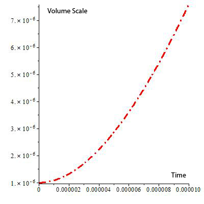
Figure 1: Evolution of the Universe given by a BVI cosmological model.

.

Fig. [1] shows the evolution of the Universe. As one sees, it is an expanding one.

IV Physical aspects of Dark energy model

Let us now find the expressions for physical quantities.

Inserting (29) into (15) and (16) one finds the expression for expansion $\vartheta$, Hubble parameter $H$:

$$\vartheta=3H=\sqrt{A_{1}V^{-(2N_{3}+6)/3N_{3}}+C_{0}/V^{2}},$$ (30)

and deceleration parameter

$$q=-\frac{A_{0}V^{-(2N_{3}+6)/3N_{3}}}{A_{1}V^{-(2N_{3}+6)/3N_{3}}+C_{0}/V^{2}}.$$ (31)

The anisotropy parameter $A_{m}$ has the expression

$$A_{m}=\frac{54(m^{2}-mn+n^{2})}{N_{3}^{2}(m+n)^{2}}.$$ (32)

The directional Hubble parameters are

$$H_{1}=\biggl{[}\frac{1}{3}-\frac{2n-m}{N_{3}(m+n)}\biggr{]}\frac{\dot{V}}{V},\quad H_{2}=\biggl{[}\frac{1}{3}-\frac{2m-n}{N_{3}(m+n)}\biggr{]}\frac{\dot{V}}{V},\quad H_{3}=\biggl{[}\frac{1}{3}+\frac{1}{N_{3}}\biggr{]}\frac{\dot{V}}{V}.$$ (33)

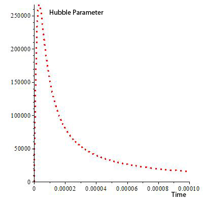
Figure 2: Evolution of the Hubble parameter

.

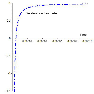
Figure 3: Evolution of the deceleration parameter.

.

Figs. [2] and [3] show the behavior of the Hubble parameter and deceleration parameter, respectively.

From (3d) we find the expression for energy density

$$\varepsilon=T_{0}^{0}=\frac{1}{\kappa}\bigl{[}X_{1}V^{-2}-X_{2}V^{-(2N_{3}+6)/3N_{3}}\bigr{]},$$ (34)

where

$$X_{1}=\biggl{[}\frac{1}{3}-3\frac{m^{2}-mn+n^{2}}{N_{3}^{2}(m+n)^{2}}\biggr{]}C_{0},\quad X_{2}=\frac{m^{2}-mn+n^{2}}{N_{0}^{2}}-\frac{X_{1}A_{1}}{C_{0}}.$$

Further we obtain

$$\omega=\frac{p}{\varepsilon}=-\frac{X_{1}-X_{4}V^{(4N_{3}-6)/3N_{3}}}{X_{1}-X_{2}V^{(4N_{3}-6)/3N_{3}}},$$ (35)

where

$$X_{4}=\frac{2N_{3}-3}{3N_{3}}A_{0}+\frac{mn}{N_{0}^{2}}-\frac{X_{1}A_{1}}{C_{0}}.$$

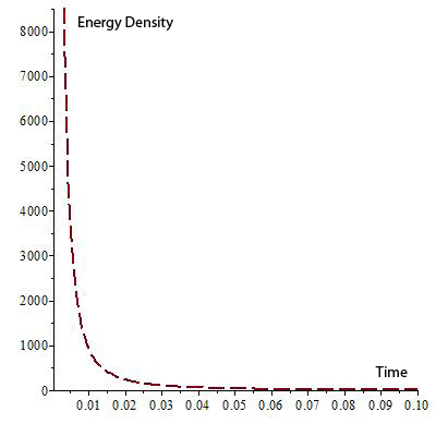
Figure 4: Evolution of the energy density

.

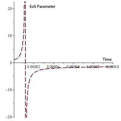
Figure 5: Evolution of the EoS parameter.

.

Figs. [4] and [5] show the behavior of the energy density and EoS parameter, respectively. As we see, energy density is a decreasing function of time, while the EoS parameter changes its sign.

So, if the present work is compared with experimental results obtained in Knop ; Tegmark1 ; Hinshaw ; Komatsu , then one can conclude that the limit of $\omega$ provided by equation (35) may accommodated with the acceptable range of EoS parameter. Also it is observed that for $V=V_{c}$, $\omega$ vanishes, where $V_{c}$ is a critical Volume given by

$$V_{c}=\biggl{(}\frac{X_{1}}{X_{4}}\biggr{)}^{3N_{3}/(4N_{3}-6)}.$$ (36)

Thus, for this particular volume, our model represents a dusty universe. We also note that the earlier real matter at $V\leq V_{c}$, where $\omega\geq 0$ later on at $V>V_{c}$, where $\omega<0$ converted to the dark energy dominated phase of universe.

For the value of $\omega$ to be in consistent with observation Knop , we have the following general condition

$$V_{1}<V<V_{2},$$ (37)

where

$$V_{1}=\biggl{(}\frac{X_{1}+1.67X_{1}}{X_{4}+1.67X_{2}}\biggr{)}^{3N_{3}/(4N_{3}-6)},$$ (38)

and

$$V_{2}=\biggl{(}\frac{X_{1}+0.62X_{1}}{X_{4}+0.62X_{2}}\biggr{)}^{3N_{3}/(4N_{3}-6)}.$$ (39)

For this constrain, we obtain $-1.67<\omega<-0.62$, which is in good agreement with the limit obtained from observational results coming from SNe Ia data Knop .

For the value of $\omega$ to be in consistent with observation Tegmark1 , we have the following general condition

$$V_{3}<V<V_{4},$$ (40)

where

$$V_{3}=\biggl{(}\frac{X_{1}+1.33X_{1}}{X_{4}+1.33X_{2}}\biggr{)}^{3N_{3}/(4N_{3}-6)},$$ (41)

and

$$V_{4}=\biggl{(}\frac{X_{1}+0.79X_{1}}{X_{4}+0.79X_{2}}\biggr{)}^{3N_{3}/(4N_{3}-6)}.$$ (42)

For this constrain, we obtain $-1.33<\omega<-0.79$, which is in good agreement with the limit obtained from observational results coming from SNe Ia data Tegmark1 .

For the value of $\omega$ to be in consistent with observation Hinshaw ; Komatsu , we have the following general condition

$$V_{5}<V<V_{6},$$ (43)

where

$$V_{5}=\biggl{(}\frac{X_{1}+1.44X_{1}}{X_{4}+1.44X_{2}}\biggr{)}^{3N_{3}/(4N_{3}-6)},$$ (44)

and

$$V_{6}=\biggl{(}\frac{X_{3}+0.92X_{1}}{X_{4}+0.92X_{2}}\biggr{)}^{3N_{3}/(4N_{3}-6)}.$$ (45)

For this constrain, we obtain $-1.44<\omega<-0.92$, which is in good agreement with the limit obtained from observational results coming from SNe Ia data Hinshaw ; Komatsu .

We also observed that if

$$V_{0}=\biggl{(}\frac{2X_{1}}{X_{4}+X_{2}}\biggr{)}^{3N_{3}/(4N_{3}-6)}.$$ (46)

then for $V=V_{0}$ we have $\omega=-1$, i.e., we have universe with cosmological constant. If $V<V_{0}$ the we have $\omega>-1$ that corresponds to quintessence, while for $V>V_{0}$ we have $\omega>-1$, i.e., Universe with phantom matter Caldwell1 .

From (34) we found that the energy density is a decreasing function of time and $\varepsilon\geq 0$ when

$$V\leq\biggl{(}\frac{X_{1}}{X_{2}}\biggl{)}^{3N_{3}/(4N_{3}-6)}.$$ (47)

In absence of any curvature, matter energy density $\Omega_{m}$ and dark energy density $\Omega_{\Lambda}$ are related by the equation

$$\Omega_{m}+\Omega_{\Lambda}=\frac{\varepsilon}{3H^{2}}+\frac{\Lambda}{3H^{2}}=1.$$ (48)

Inserting (30) and (34) into (48) we find the cosmological constant as

$$\Lambda=[3C_{0}^{2}-(X_{1}/\kappa)]V^{-2}+[3A_{1}-X_{2}/\kappa]V^{-2(N_{3}+3)/3N_{3}},$$ (49)

As we see, the cosmological function is a decreasing function of time and it is always positive when

$$V\geq\biggl{(}\frac{X_{1}/\kappa-3C_{0}}{3A_{1}-X_{2}/\kappa}\biggr{)}^{3N_{3}/(4N_{3}-6)}.$$ (50)

Recent cosmological observations suggest the existence of a positive cosmological constant $\Lambda$ with the magnitude $\Lambda(G\hbar/c^{3})\approx 10^{-123}$. These observations on magnitude and red-shift of type Ia supernova suggest that our universe may be an accelerating one with induced cosmological density through the cosmological $\Lambda$-term. Thus, the nature of $\Lambda$ in our derived DE model is supported by recent observations. Fig. [6] shows the evolution of the cosmological constant. As is seen, it is a decreasing function of time.

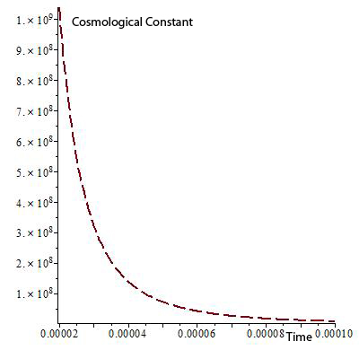
Figure 6: Evolution of the cosmological constant

.

For the stability of corresponding solutions, we should check that our models are physically acceptable. For this, the velocity of sound is less than that of light, i.e.,

$$0\leq v_{s}=\frac{dp}{d\varepsilon}<1.$$ (51)

In this case we find

$$v_{s}=\frac{dp}{d\varepsilon}=-\frac{X_{1}-[(N_{3}+3)X_{4}/3N_{3}]V^{(4N_{3}-6)/3N_{3}}}{X_{1}-[(N_{3}+3)X_{2}/3N_{3}]V^{(4N_{3}-6)/3N_{3}}}.$$ (52)

Fig. [7] shows the behavior of $v_{s}$ in time.

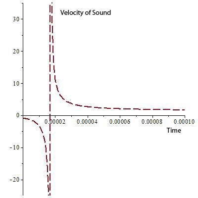
Figure 7: Speed of sound with respect to cosmic time

.

As one sees, there are regions, where the solution is stable. Choosing the problem parameters, such as $m,n,N_{3}$ we can obtain the stable solutions.

V Conclusion

In this report we have studied the evolution of the universe filled with dark energy within the scope of a Bianchi type-VI model. In case of a BVI model we found the exact solutions to the field equations in quadrature. It was found that if the proportionality condition is used, this together with the non-diagonal Einstein equation leads to the isotropic distribution of energy momentum tensor, i.e., $T_{1}^{1}=T_{2}^{2}=T_{3}^{3}$. This fact allows one to solve the equation for volume scale $V$ exactly. The behavior of EoS parameter $\omega$ is thoroughly studied. It is found that the solution becomes stable as the Universe expands.

References

• (1) Amirhashchi H., Pradhan A., and Saha B., Astrophys. Space Sci. 333 295 (2011).
• (2) Amirhashchi H., Pradhan A., and Saha B., Chinese Phys. Lett. 3 039801 (2011).
• (3) Ib$\acute{a}\tilde{n}$ez J., van der Hoogen R.J., Coley A.A., Phys. Rev. D 51 928 (1995).
• (4) Caldwell R.R., Phys. Lett. B 545 23 (2002).
• (5) Hinshaw, G., et al., Astrophys. J. (Suppliment Series) 180 225 (2009).
• (6) Kantowski R. and Sachs R.K., J. Math. Phys. 7 443 (1966).
• (7) Kristian J. and Sachs R.K., Apstrophys. J. 143 379 (1966).
• (8) Knop R.K., et al., Astrophys. J. 598 102 (2003).
• (9) Komatsu, E., et al., Astrophys. J. (Suppliment Series) 180 330 (2009).
• (10) Pradhan A., Amirhashchi H., and Saha B., Int. J. Theor. Phys. 50 2923 (2011).
• (11) Pradhan A., Amirhashchi H., and Saha B., Astropys. Space Sci. 333 343 (2011).
• (12) Saha B., Phys. Rev. D 69 124006 (2004).
• (13) Saha B., Gravitation $\&$ Cosmology 16 160 (2010).
• (14) Saha B., Amirhashchi H., and Pradhan A., Astrophys. Space Sci. 2012 (online first)
• (15) Saha B. and Visinescu M., Romainan J. Phys. 55 1064 (2010).
• (16) Socorro J., Medina E.R., Phys. Rev. D 61 087702 (2000).
• (17) Tegmark, M.,et al., Phys. Rev. D 69 103501 (2004).
• (18) Thorne K.S., Astrophys. J. 148 51 (1967).
• (19) Weaver M., Classical Quant. Grav. 17 421 (2000).
• (20) Yadav A.K. and Saha B., Astrophys. Space Sci. 337 759 (2012).