The return of the Andromedids meteor shower

Abstract

The Andromedid meteor shower underwent spectacular outbursts in 1872 and 1885, producing thousands of visual meteors per hour and described as ‘stars fell like rain’ in Chinese records of the time Kronk (1988); Nogami (1995). The shower originates from comet 3D/Biela whose disintegration in the mid-1800’s is linked to the outbursts, but the shower has been weak or absent since the late 19th Century.

This shower returned in December 2011 with a zenithal hourly rate of approximately 50, the strongest return in over a hundred years. Some 122 probable Andromedid orbits were detected by the Canadian Meteor Orbit Radar while one possible brighter Andromedid member was detected by the Southern Ontario Meteor Network and several single station possible Andromedids by the Canadian Automated Meteor Observatory.

The shower outburst occurred during 2011 Dec 3-5. The radiant at RA +$18^{\circ}$ and Dec +$56^{\circ}$ is typical of the ‘classical’ Andromedids of the early 1800’s, whose radiant was actually in Cassiopeia. The orbital elements indicate that the material involved was released before 3D/Biela’s breakup prior to 1846. The observed shower in 2011 had a slow geocentric speed (16 km s^-1) and was comprised of small particles: the mean measured mass from the radar is $\sim 5\times 10^{-7}$ kg corresponding to radii of 0.5 mm at a bulk density of $1000$ kg/m³.

Numerical simulations of the parent comet indicate that the meteoroids of the 2011 return of the Andromedids shower were primarily ejected during 3D/Biela’s 1649 perihelion passage. The orbital characteristics, radiant, timing as well as the absence of large particles in the streamlet are all consistent with simulations. Predictions are made regarding other appearances of the shower in the years 2000-2047 based on our numerical model. We note that the details of the 2011 return can, in principle, be used to better constrain the orbit of 3D/Biela prior to the comets first recorded return in 1772.

1 Introduction

“We can only hope that future perturbations will again switch the group [Andromedids] across our path, so that more can be learned of the processes at work related to the evolution and disintegration of the comet and how far they have progressed.” Oliver (1925)

In 1845/46, comet 3D/Biela was observed to be in the process of fragmenting, a process which continued until the comet disappeared entirely following its 1852 return. The break-up was followed by a strong shower (the Andromedids), a shower first reported in 1798 and displaying spectacular outbursts in 1872 and 1885 during which thousands of meteors per hour were reported Kronk (1988); Nogami (1995). The shower has decreased in intensity since that time and since the early 20th century rates are less than a few per hour Hawkins et al. (1959).

Comet 3D/Biela was a Jupiter-family comet first discovered in March 1772 by J. L. Montaigne Kronk (1999). This comet is significant for being the first comet to be ‘lost’ and acquire the ‘D’ designation instead of the usual ‘P’ designation of periodic comets. It is also among the first comets to be linked to meteor activity, as Weiss, d’Arrest and Galle all independently reported the link between the Andromedid shower and Biela’s orbit Kronk (1988).

According to Jenniskens (2006) and Hawkins et al. (1959), probable returns of the Andromedids date back to roughly the mid-18th Century. Observations of the stream from the mid-18th to mid-19th century report the time of maximum to be in the first week in December, while the major storms of 1872 and 1885 occurred on Nov 27. Moreover, the few reports of strong activity from the shower in the late-18th Century have times of maximum progressively earlier, including Nov 24, 1892 and 1899; Nov 22, 1904 and finally Nov 15, 1940 when the last activity at a level of a few tens of meteors per hour was noted. Hawkins et al. (1959) describes annual activity from the stream visible in the mid-20th century among Super-Schmidt camera meteor data, but of weak intensity. The decreasing times of maximum reflect the change in the nodal longitude of the 3D/Biela and the increasingly young trails encountered in later years. From Jennisken’s 2006 compilation (see his Table 6a), the apparent radiant of the shower has moved in concert with the changing date of maximum. The earliest showers, having maxima in December/very late November had radiants near RA=$+20^{\circ}$ and Dec=$+50^{\circ}$ to $+60^{\circ}$ while the later showers (1850 onwards) and the storms of 1872/1885 had radiants of RA=$+27^{\circ}$, Dec=$+44^{\circ}$. It is this latter era of the shower activity, punctuated by the storms of 1872/1885 with the radiant in Andromeda which gave the shower its modern name. In fact, the first measurements of the shower showed the radiant to be in Cassiopeia, a feature of the shower long recognized (e.g. Oliver (1925)). The change in the radiant in concert with the date reflects the very different epochs of ejection from 3D/Biela and its changing orbit through different eras.

The link between the Andromedids and Biela was examined most recently by Jenniskens and Vaubaillon (2007). They studied the outbursts of the 19th century in order to determine whether they were primarily the result of material released during the splitting event or by the usual process of water vapour sublimation, and conclude that ongoing fragmentation particularly during the 1846 passage after the splitting event is most likely responsible for the 1872 and 1885 outbursts. Confining their ejection epochs to perihelion passages of the comet after 1703, they were able to model quite a number of appearances of the Andromedids through to 1940.

However, a few occurrences of observed showers did not appear in their simulations: these may have been produced by perihelion passages of the comet prior to 1703, the first perihelion they consider. They did not examine possible appearances of the shower in the current era.

Here we describe the first modern, strong return of the Andromedid shower occurring during 2011 Dec 3-5. Section 2 describes the observations of the meteor shower, Section 3 outlines the simulations and Section 4 presents a comparison of the two. Conclusions are drawn in section 5.

2 Observations

The first indication of unusual activity associated with the Andromedids in 2011 was made during post-processing of radar measurements conducted by the Canadian Meteor Orbit Radar (CMOR) as part of a program aimed at detecting brief shower outbursts. The Canadian Meteor Orbit Radar is a multi-station, backscatter radar system operating at 29.85 MHz which is able to measure trajectories and speeds for individual meteors. Details of the basic system can be found in Webster et al. (2004); Jones et al. (2005); Brown et al. (2008) and Brown et al. (2010b). The original CMOR system began orbital measurements in 2001 using a three station setup. In mid-2009, CMOR was upgraded to higher transmit power (12 kW from 6 kW) and three additional remote stations were added to the facility. In this new configuration, the number of measured orbits has increased from 2000-3000 per day (with the original CMOR) to $\sim 5000$ per day with CMOR II. Additionally, many orbits now have more than three station detections, and so the accuracy of the overall orbital measurements has improved.

Our meteor outburst survey follows the methodology previously employed to detect longer-lived showers in CMOR orbital data by using a 3-dimensional wavelet transform (see Brown et al. (2010b) for details). All potential single day maxima detected by this approach in CMOR data are correlated with known showers based on the original CMOR shower catalogues Brown et al. (2008, 2010b) and the working list of meteor showers maintained by the International Astronomical Union. We find that CMOR detects 1-2 outbursts each year, defined as either unknown, intense, short-lived showers or significant enhancements over normal activity from among previously known annual streams. Among the former category was the detection of the Daytime Craterids in 2003 and 2008 Wiegert et al. (2011) while the latter type of outburst is well represented by the October Draconids in 2005 Campbell-Brown et al. (2006). Full details of this complete outburst survey will be published separately. Here we present details of the detection of the Andromedids in 2011 as a separate study due to its unusual nature and intensity. In Table LABEL:ta:radar2011 we list the top three strongest radiants detected by CMOR II using our wavelet technique between solar longitudes $\lambda=250-252^{\circ}$ in 2011 (Dec 3-5). In all previous years either the NOO (November $\omega$ Orionids) or GEM (Geminids) were by far the dominant radiants during this interval. The intensity of the shower is best represented by $N\sigma$, the number of standard deviations the wavelet coefficient is above the median background. Our normal single-day strength cutoff establishing a probable shower maximum point is $8\sigma$. For comparison, the Draconid outburst in 2005 produced an $N\sigma$ of 39 and the Daytime Craterid outbursts an $N\sigma$ of 36 and 33 in 2003 and 2008 respectively. During the 10 years of CMOR operation, other than these showers, only the Andromedid return in 2011 has exceeded a threshold of 30 $\sigma$ for a single day outburst. Note that in Table LABEL:ta:radar2011 the strong radiant was not automatically identified with the traditional Andromedid shower due to large differences in the radiant; this disparity is explained in the modelling section.

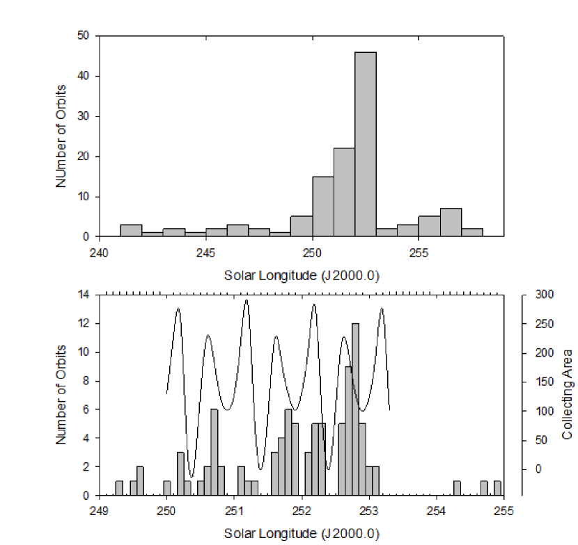
Figure 1: CMOR’s 2011 Andromedid meteor orbit count as a function of solar longitude. The bottom panel also displays the (time-varying) collecting area in square km. Note that there was a loss in transmitting power (and hence meteor counts) due to freezing rain beginning at $253.3^{\circ}$ until $254.1^{\circ}$.

$\lambda$ (J2000) RA (^∘) Dec (^∘) V_g (km s^-1) $N\sigma$ $N_{orb}$ desig 250 92.8 +15.9 42.9 33.7 459 NOO 20.2 +54.1 16.2 14.5 45 100.4 +34.6 33.6 12.9 380 GEM 251 93.6 +15.4 42.9 25.1 399 NOO 19.9 +56.9 17 22.1 38 101.7 +34 33.6 18.2 343 GEM 252 18.2 +57.5 16.2 30.6 63 102.7 +34.5 33.6 16.6 314 GEM 94.1 +14.4 40.8 14.9 296 NOO

Table 1: The top three wavelet peaks in 2011 and associated showers from solar longitudes $\lambda$ from $250^{\circ}-253^{\circ}$. $V_{g}$ is the geocentric velocity, $N\sigma$ represents the number of standard deviations of the wavelet detection above the usual background, and $N_{orb}$ is the number of orbits used to compute the wavelet coefficient. Two other showers are active at this time: GEM is the Geminids, NOO is the November $\omega$ Orionids: the lines without an entry in the designation column list the data for the 2011 Andromedids outburst reported here. Radiants are geocentric J2000.

The peak activity appears to have occurred between $\lambda=252^{\circ}-253^{\circ}$, most likely between $\lambda=252.7^{\circ}-252.8^{\circ}$ (9-12 UT, Dec 5) based solely on the number of orbits recorded from the shower (Figure 1). The absolute peak flux at this time was equivalent to a zenithal hourly rate (ZHR) of approximately 50. The increase in numbers during this period is probably significant given that the collecting area of the radiant at the time of maximum as seen by CMOR II decreases by 40% compared to the previous two hour interval. However, whether the outburst continued through the next day is uncertain as a period of freezing rain began near 0 UT Dec 6 ($\lambda=253.2^{\circ}$) and this led to the radar automatically shutting off (due to high TX power reflection) until 18.5 UT Dec 6 (254.1^∘). Certainly the activity did not extend significantly into the $\lambda=254^{\circ}$ range, but we have almost no radar observations (due to the weather and low radiant collecting area) during $\lambda=253^{\circ}-254^{\circ}$. In total, 122 probable Andromedid orbits were recorded during the interval from $\lambda=240^{\circ}-260^{\circ}$, the majority (85) occurring between $\lambda=250^{\circ}-253^{\circ}$. By way of comparison, between $\lambda=250^{\circ}-253^{\circ}$ the average number of radiants within 10 degrees of this location having similar speeds between 2001 - 2010 was $\sim 10$ per year. Figure 2a shows all $\sim 14000$ measured radiants in 2011 detected by CMOR II between $\lambda=250^{\circ}-253^{\circ}$ in sun-centred ecliptic coordinates as a Mercator projection; a polar projection is in Figure 2b. The clump of Andromedid radiants is obvious to the eye: it particularly stands out from the background because of the very low radiant density at such a large elongation from the Earth’s apex. Also labelled are the Geminid and November $\omega$ Orionid radiants. From the cumulative amplitude distribution of the 122 echoes from the Andromedid radiant, we follow the basic technique outlined in Blaauw et al. (2011) to compute a shower mass distribution index. The mass index $s$ is the power-law exponent in the differential relation presumed to hold between the cumulative number of meteoroids of mass $m$ or larger and their number such that $dN=m^{-s}dm$ (see Ceplecha et al. (1998) for a complete description). Note that unlike the single-station selection technique used in Blaauw et al. (2011) which necessarily includes substantial contamination from other radiants, we are able to select only those radiants associated with the shower. We find $s=2.2$ for the stream, substantially higher than found for other major streams with CMOR, suggesting strongly that the outburst was rich in fainter meteors.

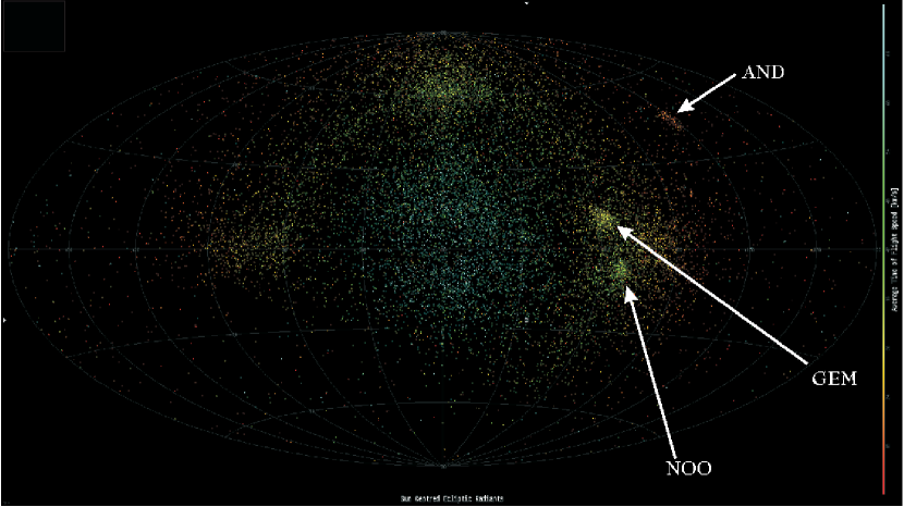
Figure 2a: CMOR radiants detected between solar longitudes of $250^{\circ}-253^{\circ}$, plotted in a Sun-centered ecliptic reference frame. The apex of the Earth’s motion is at the centre of the plot. The color coding is apparent velocity.

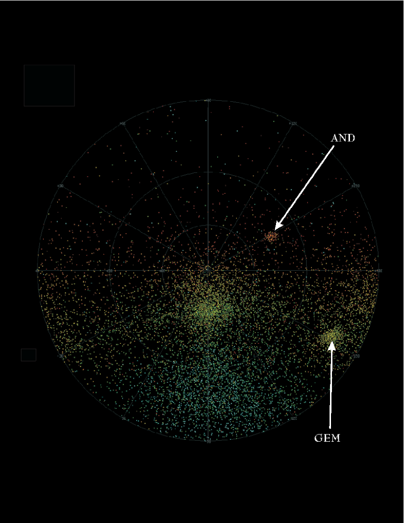
Figure 2b: CMOR radiants detected between solar longitudes of $250^{\circ}-253^{\circ}$, plotted in a Sun-centered ecliptic reference frame, looking down on the north ecliptic pole (center).

Figure 3: Geocentric right ascension and declination for all radiants (open circles) and for the highest quality radiants (black circles with errors) from CMOR. See the text for more details.

The radiant of all 122 probable Andromedids is shown in Figure 3. Note that the errors per radiant are found using a Monte Carlo technique which adds Gaussian noise to an idealized model echo having the same set of signal-to-noise ratios, decay times, heights and nominal time offsets at each outlying station as the observed echo and then chooses the inflection time picks and performs interferometry using the same algorithms used to process real data, as described in Weryk and Brown (2012). The resulting errors represent the standard deviation of the radiant position computed per orbit among these simulations. This approach captures the large errors often associated with poor geometry in the multi-station reflection process. To better define the shower, we further select only those echoes having errors in semi-major axis less than 20% of the semi-major axis value, according to the Monte Carlo process. This amounts to $\sim 50$ orbits total; of these, 90% are in the $250^{\circ}-253^{\circ}$ interval. The radiant distribution for this high quality orbit group is shown as well in Figure 3. It is clear that there is a tight radiant near RA=18^∘ and Dec=$+56^{\circ}$, with a spread of order $5^{\circ}$. Note that we have not corrected for any radiant drift in this plot of observed geocentric radiant positions; hence some of this spread is simply due to drift. Interestingly, as part of the outburst survey, we also detected a relatively strong single day maximum on November 27, 2008 associated with the Andromedids (but at a lower declination than the 2011 outburst) - this is shown in Table LABEL:ta:radar2008. The number of radiants associated with this detection is small (30) and the shower strength is lower than in 2011. This matches a weak shower seen in the simulations, discussed in section 4.

$\lambda$ (J2000) RA (^∘) Dec (^∘) V_g (km s^-1) $N\sigma$ $N_{orb}$ CMOR 246 26.6 +44.4 15.9 11.5 30 Simulation 251.6 28.8 +47.4 16.0 - 77

Table 2: CMOR and simulation data for the 2008 Andromedid shower. See Table LABEL:ta:radar2011 for more details.

In addition to the CMOR observations, the Southern Ontario Meteor Network Brown et al. (2010a) detected one possible member of the outburst on Dec 3 at 04:24 UT of magnitude -1. Note that Dec 3 was the only clear night in the interval 2011 Dec 3 - 8 in southern Ontario. On the same night, a single station of the Canadian Automated Meteor Observatory (CAMO) Weryk et al. (2012) recorded 3 possible members of the outburst between 0530 - 0730 UT Dec 3, all fainter than +4. These optical observations are consistent with the outburst being generally rich in faint meteors as suggested by the steep mass index measured by the radar.

It is worth noting that the radiant of the 2011 shower reported here is more typical of the ‘early’ Andromedids of the 19th century, a December shower whose radiant is near RA $=+20^{\circ}$, Dec $=+54^{\circ}$ (actually in Cassiopeia) rather than the ‘modern’ Andromedids, a November shower whose radiant is near RA $=+25^{\circ}$ Dec $=+44^{\circ}$. Precession of the meteoroid stream has resulted in the displacement of the classical stream to its current position. Nonetheless, simulations (described later) reveal that some slowly-precessing material released from 3D/Biela in the 17th century is responsible for the outburst seen in 2011.

3 Simulations

In order to better understand the nature of the 2011 outburst, numerical simulations were performed of the parent comet. Simulations of meteoroids released during each of Biela’s perihelion passages up to 200 years prior to its discovery were examined for clues as to the origin of the material that produced the 2011 outburst. The properties of the outburst in 2011 could be used to better refine earlier orbits for 3D/Biela, though we are looking only for coarse agreement to establish the broad strokes of the origin and evolution of the streamlet seen in 2011.

The meteoroids were simulated within a Solar System of eight planets whose initial positions and velocities were determined from the JPL DE406 ephemeris Standish (1998). The particles were integrated with a symplectic integration code Wisdom and Holman (1992) which handles close encounters by the Chambers (1999) method. Some simulations were duplicated with the RADAU method Everhart (1985) and the results were found to be qualitatively the same. The speed of the symplectic code allowed roughly ten times as many particles to be simulated, and these ‘higher-resolution’ results are reported here. The Earth-Moon are simulated as a single particle at the Earth-Moon barycenter. A time step of 7 days is used in all cases.

The simulations were also run with a novel two-stage refinement procedure. First we describe the initial stage, which parallels the usual approach to such studies. The comet orbit is integrated backwards to the desired starting point, 200 years prior to the comet’s discovery. The comet is then integrated forward again, releasing meteoroids at each perihelion passage as it does so. The methodology of Vaubaillon et al. (2005) is followed whereby the size distribution can be taken into account by applying a statistical weight to the particles based on their mass index after the simulations are completed. In our simulations, at each perihelion passage a number $M=1000$ particles is released in each of the four size ranges of $10^{-5}-10^{-4}$ m, $10^{-4}-10^{-3}$ m, $10^{-3}-10^{-2}$ m and $10^{-2}-10^{-1}$ m, extending from 10 microns to 10 cm in diameter, so that the distribution of particle radii is flat when binned logarithmically. The simulations include post-Newtonian GR corrections and radiative ($i.e.$ Poynting-Robertson) effects. The ratio of radiative to gravitational force $\beta$ is related to the particle radius $r$ (in $\mu$m) through $\beta=0.57/r$ following Weidenschilling and Jackson (1993), where we use a particle mass density $\rho=1000$ kg m^-3.

The comet is considered active (that is, simulated meteoroids are released) when at a heliocentric distance of 3 AU or less. While active, particles are released from the parent comet in time from a uniform random distribution, with velocities from the prescription of Crifo and Rodionov (1997). Lacking specific information about the nucleus of comet Biela (e.g. Tancredi et al. (2000)), the Bond albedo of the comet nucleus is taken to be 0.05, the nucleus and meteoroid densities $1000$ kg m^-3, the nucleus radius 1000 m, and the active fraction of the comet’s surface, 20%.

The comet and all meteoroids are integrated until the simulation’s end point. The output is searched, and all meteoroids which pass sufficiently close to the Earth’s orbit during the period of time in question are extracted and examined: this is our list of “bulls-eyes”. This is the end of the first stage of the simulations and to this point, the process follows the commonly-accepted procedure for studying meteor showers.

The next stage refines the results by concentrating on those meteoroids which are able to reach the Earth. Such methods have been used before with great success. Wu and Williams (1996), Asher (1999) and McNaught and Asher (1999) used the fact that the orbit of comet 55P/Tempel-Tuttle evolves only slowly to preferentially select Leonid shower meteoroids that would impact the Earth for simulation, at a considerable saving in computational time. Our method is similar but does not require the parent orbit to be slowly evolving in time. Rather, in our refinement stage, the list of “bulls-eyes” is used to populate a second set of simulations. In this second set, the parent comet is integrated in exactly the same manner as in the first stage, except that this time meteoroids are only ejected near the initial conditions known to produce bulls-eyes in the first simulation.

The details of the second stage procedure used are as follows. At each time step during the second simulation, a check was made to see if a “bulls-eye” was produced in the same time step in the first simulation. If so, $N$ new particles with orbits similar to the bulls-eye are produced, where the calculation of $N$ is discussed below. All particles have the same position (that of the nucleus, taken to be a point particle). Each component of the meteoroid’s velocity vector relative to the nucleus is given a random kick of up to $\pm 10$% of that of the original bulls-eye, as is its $\beta$. These “second generation” particles (and any others that are produced in later time steps by other bulls-eyes) are then integrated forward in the usual way. At the end of the simulation, those meteoroids which pass near the Earth at the time under investigation are extracted. Invariably, these contain far more meteoroids than the bulls-eye list of the initial simulation. As a result, a much clearer look at the regions of phase space which produce the shower event in question is obtained at relatively low computational cost.

The number $N$ of particles produced near a given bulls-eye is calculated as follows. Let $M$ (always taken to be 1000 here) be the number of particles released in a given perihelion passage in each of the four size bins. If there were $n$ bulls-eyes recorded in that particular size bin during the current perihelion passage then each is assigned a fraction $1/n$ of the $M$ particles assigned ($N=M/n$). For example, if there are 10 bulls-eyes of sizes from $10^{-5}$ to $10^{-4}$ m in the first simulation, then the region near each of those 10 will be seeded with $M/10=100$ particles in the second-generation. If there had been 100 bulls-eyes in this perihelion and size bin, then each bulls-eye would have been seeded with $M/100=10$ particles in the second generation. Typically $\sim 1$% particles released in the first generation hit the Earth, and so each bulls-eye is usually reseeded by $\sim 100$ particles.

This procedure is adopted, instead of say, simply replacing each bulls-eye with a fixed number of particles because 1) it maintains a constant computational load from simulation to simulation and 2) it favours perihelion passages which produce few meteors: this hopefully allows us to avoid missing possibly-rich perihelion passages that might have been missed by the granularity of the first simulation. The procedure adopted does make it slightly more complicated to convert from the number of simulated meteors in a shower event to the actual number, but this is easily accomplished by assigning a weight to each simulated meteor that is proportional to $1/N$.

The effects of granularity in the first simulation are worth noting. If a given perihelion passage produces no bulls-eyes in the initial simulation, then at the refinement stage, no meteors at all will be released during that passage. Thus the first simulation must sample the available phase space well enough (i.e. $M$ must be large enough) or the refinement procedure will fail. It appears empirically that our choice of $M=1000$ is sufficient to meet this condition in this case, but the possibility that important regions of meteoroid ejection phase space have been missed remains.

The list of bulls-eyes at the end of the first stage would ideally consist entirely of particles which physically collide with the Earth; however current computational limits prevent simulating the number of particles needed to produce a statistically significant number of such collisions. Thus we are forced to select our criteria more generously and somewhat arbitrarily, though guided by experience. Here we have required a bulls-eye to satisfy two criteria 1) the minimum orbital intersection distance between the meteoroid’s orbit and the Earth’s orbit should be less than 0.1 AU. Note that we do not use a nodal distance but a true minimum in the inter-orbit distances. Though more laborious to compute, it is more robust in the case of low-inclination orbits where the node may be located a large distance from the closest point of approach. 2) The meteoroid should be at its closest approach to Earth within $\pm 30$ days of the shower date, here taken to be December 4th 0h UT. Thus the bulls-eye criteria specifically select those meteoroids which are closest to Earth during the meteor shower one is modelling, out of all the meteoroids simulated, of all sizes, from all perihelion passages simulated.

An auxiliary simulation was performed in which the comet orbit was integrated backwards for a thousand years in order to determine its Lyapunov exponent using the algorithm of Mikkola and Innanen (1999). This measure of the chaotic time scale is necessary to understand over what interval we can have confidence in our simulations. The $e$-folding time of Biela was found to be $\approx 25$ years. This short Lyapunov time is typical of a Jupiter-family comet that has numerous close approaches to that giant planet. We find that in our simulations Biela’s 1772 orbit, when integrated back 200 years, has close encounters ($\leq 5$ Hill radii) with Jupiter in 1747, 1711, 1664, 1652 and 1604. The last in 1604 is at $\approx 1.2$ Hill radii. Thus our backwards integrations of 200 years go back eight Lyapunov times, which stretches the limits of what we expect chaos to allow us to calculate reliably, and so we do not attempt to go further back. Note that the timing, particle population and radiant of the observed trailet in 2011 may actually allow a better refinement of the early orbit for 3D/Biela, though such a study is beyond the scope of the current work. Using the timing and characteristics of contemporary showers with known ejection age as a means to potentially constrain the early orbit of a parent comet has been discussed before (e.g. Vaubaillon et al. (2011)).

The comet orbital elements used in these simulations are derived from Marsden and Williams (2008). No non-gravitational forces due to outgassing (e.g. Marsden et al. (1973)) were applied. Because the comet orbit evolved significantly during the 80 years between when it was discovered (1772) and the last observation of the fragments (1852) we did not use a single set of orbital elements for the comet. Rather, the 1772 discovery orbit was used as the starting point for all perihelion passages prior to this time back 200 years to 1572. The perihelion passages from 1772 to 1852 were modelled in parallel three times, using the orbit of 1832, as well as the final orbits of fragments A and B from 1852, their last apparition. These are all listed in Table LABEL:ta:elements. The multiple models for the end of comet Biela’s lifetime allow a careful exploration of the phase space since the dynamical effects of fragmenting and additional outgassing, not to mention the ever-present perturbations due to Jupiter, make the simulation of this very interesting part of Biela’s life difficult. We will see that the different fragment orbits produce different results, as will be discussed in more detail in section 4.

n Name Peri date $q$ (AU) $e$ pd (yr) $\omega$ (^∘) $\Omega$ (^∘) $i$ (^∘) 1 3D/1772 E1 1772 Feb. 17.675 0.99038 0.72588 6.87 213.340 260.942 17.054 2 3D/1832 S1 1832 Nov. 26.6152T 0.879073 0.751299 6.65 221.6588 250.6690 13.2164 3 3D-A 1852 Sept. 23.5432T 0.860594 0.755828 6.62 223.1890 248.0070 12.5488 4 3D-B 1852 Sept. 24.2212T 0.860625 0.755879 6.62 223.1912 248.0043 12.5500

Table 3: A list of the orbital elements used for comet Biela and its fragments in this paper. From Marsden and Williams (2008).

4 Simulation results and comparison with observations

The simulation output for the year 2011 are presented in Fig. 4a, which shows the nodal intersection points of the simulated meteoroids overplotted on the Earth’s orbit. A band of meteoroids from the 1649 perihelion passage (as determined from the backward integration of the 1772 orbit of 3D/Biela) sits astride the Earth’s orbit, along with a smaller grouping from the 1758 passage (see Fig. 4b). The timing of the arrival of these particles matches well with the CMOR observations (Fig. 5) particularly when the loss of radar sensitivity due to transmitter icing near $\lambda\approx 253-254^{\circ}$ is considered. As a result of this match, we conclude that the 2011 appearance of the Andromedids resulted from dust produced by the 1649 perihelion passage of the parent comet, and other details (discussed below) support this result.

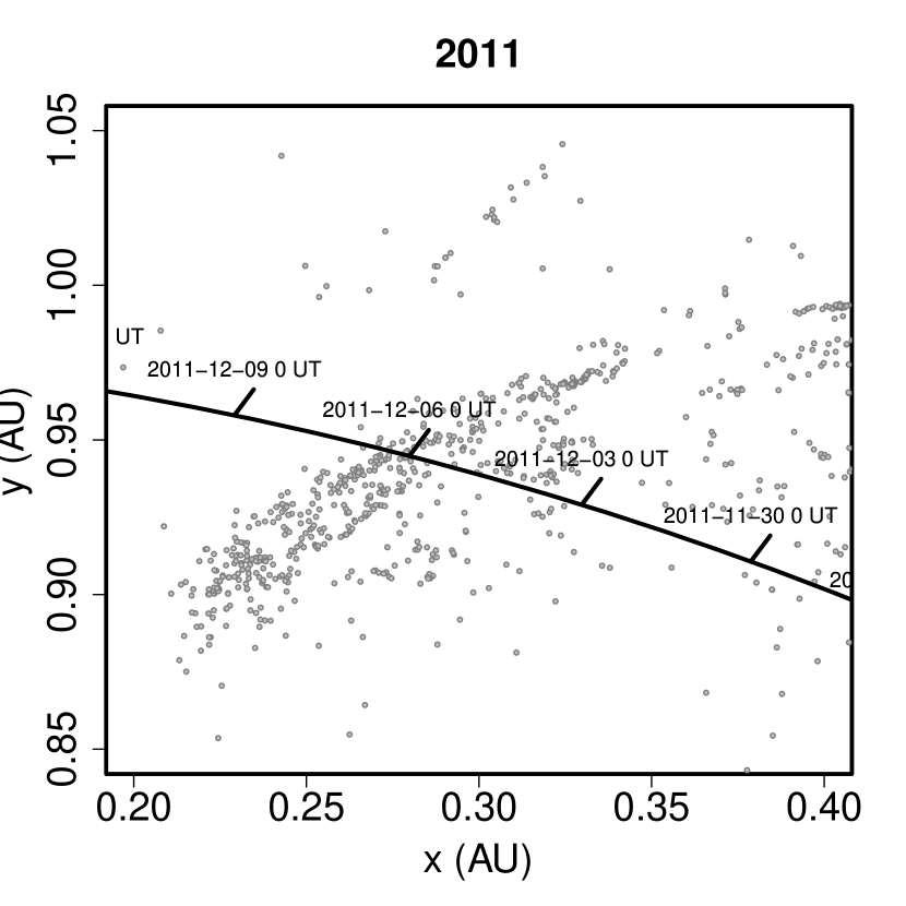
Figure 4a: The nodal intersection points of simulated meteoroids arriving at the Earth in 2011. The Earth’s orbit is the heavy black curve with the time of the planet’s passage labelled.

Figure 4b: The nodal intersection points of simulated meteoroids arriving at the Earth in 2011, identified by the perihelion passage when they were produced.

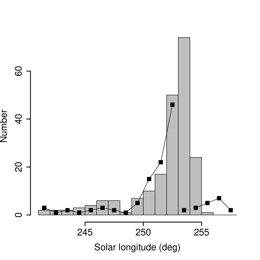
Figure 5: Counts of Andromedids meteors seen by CMOR (black squares) together with those of simulated meteoroids passing no more than 0.01 AU from Earth’s orbit (grey histogram). A gap in the black line connecting the CMOR data at solar longitudes 253-254^∘ indicates the loss of sensitivity due to antenna icing.

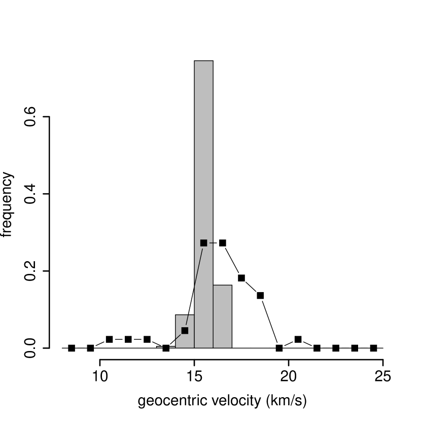
Figure 6: The measured geocentric velocities of the 44 highest quality Andromedids measured by CMOR (black squares) and the simulated 2011 Andromedids (grey histogram).

The velocity of the CMOR-observed meteors is shown in Figure 6, as are those of the simulations. They are consistent with each other, both concentrated near 16 km s^-1 though there is more spread in the radar data as would be expected from measurement errors.

The size distribution is also qualitatively consistent with CMOR observations. The simulated size distribution at Earth is concentrated at small sizes, with no particles larger than 100 $\mu$m though our simulations include particle with radii up to 10 cm. CMOR saw particles which were somewhat larger than this: the typical sizes for CMOR-detected Andromedids is 500 $\mu$m at an assumed density of 1000 kg/m³ but the steep measured mass index of $s=2.2$ (see Section 2) is consistent with a shower rich in small meteors over larger ones.

The radiants are shown in Fig. 7. The locations of the simulated and observed radiants differ by about $\sim 8$ degrees. This likely reflects the remaining uncertainty in 3D/Biela’s orbit in 1649 compared to our adopted orbit as well as uncertainty in our deceleration correction for the observed meteors between observed in-atmosphere and estimated out-of-atmosphere speeds (Brown et al., 2004). In the simulations, two different radiants separated by a few degrees are seen, one originating from the 1649 perihelion passage, the other from 1758. The mean orbits of the two simulated radiants are shown in Table LABEL:ta:radiants: the numbers are similar though not identical.

Figure 7: The right ascension and declination of the highest quality radiants from CMOR (open circles with error bars) along with the simulated radiants for the 2011 Andromedids (black circles). The ellipses show two standard deviations in RA and Dec for both radiants.

Name RA (^∘) Dec (^∘) $a$ (AU) $a_{\beta=0}$ (AU) $q$ (AU) $e$ $i$ (^∘) $\Omega$ (^∘) $\omega$ (^∘) CMOR 18.2 57.4 3.78 3.81 0.902 0.76 18.3 253.5 216.3 $\pm$ 2.6 2.2 0.71 0.71 0.012 0.04 1.0 2.4 3.1 Sim: all 23.6 +50.2 3.78 3.40 0.894 0.763 14.5 252.5 218.1 $\pm$ 2.5 1.3 0.12 0.17 0.011 0.007 0.4 2.1 1.9 Sim: 1649 24.9 +50.7 3.70 3.44 0.891 0.759 14.7 253.7 218.5 $\pm$ 1.1 0.4 0.02 0.18 0.007 0.001 0.2 0.6 0.8 Sim: 1758 21.2 +49.2 3.91 3.31 0.905 0.769 14.1 250.7 217.2 $\pm$ 0.9 1.2 0.04 0.08 0.007 0.003 0.2 1.8 1.8

Table 4: Numerical values for the radiants shown in Fig. 7. The line beginning with $\pm$ indicates one standard deviation in the quantities above it. Note that the orbital elements take into account the effect of radiation pressure which is non-negligible for some particles ( $\beta\mathrel{\hbox{\hbox to0.0pt{\hbox{\lower 3.0pt\hbox{$\sim$}}\hss}\hbox{\raise 2.0pt\hbox{$<$}}}}10^{-2}$). The orbital element most sensitive to $\beta$ is the semimajor axis $a$: its value under the assumption of $\beta=0$ is shown in the column labelled $a_{\beta=0}$ for comparison

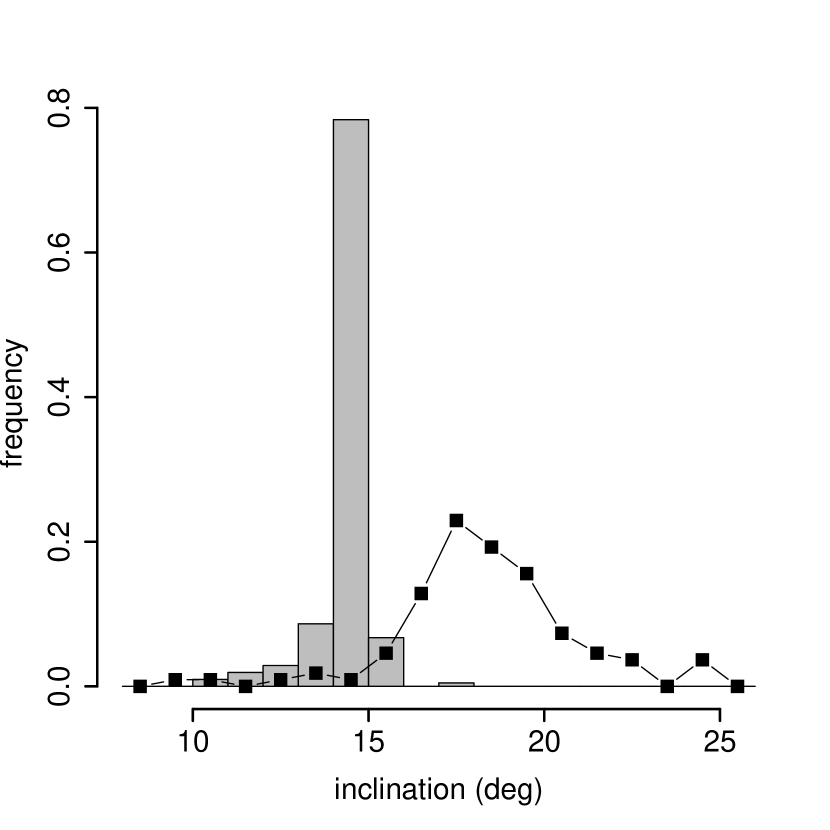
Figure 8: The CMOR-measured (black squares) inclinations along with those of the simulated (grey histogram) Andromedids.

The inclination distribution is shown in Fig. 8; along with the observed distribution. The observed is slightly higher in inclination on average (by about 3^∘), but again, such small deviations may reflects the remaining uncertainty in 3D/Biela’s orbit in 1649 compared to our adopted orbit compounded by our uncertainty in deceleration correction.

Given the nodal footprint of the 1649 perihelion passage, the similarity of the times of arrival to observations, and the match between the radar derived sizes, radiants and inclinations and those of the simulations, we conclude that the 2011 Andromedids shower can be traced primarily to the release of material by comet Biela during its 1649 perihelion passage and that the shower is due to small particles released during that passage having unusually favourable dynamical delivery efficiencies to the Earth in 2011.

The meteoroids which reach the Earth from the 1649 perihelion passage come primarily from the pre-perihelion leg rather than post-perihelion (3:1 ratio), though they are otherwise distributed throughout the comet’s active phase ($r<3$ AU).

The 2011 shower is more like the early appearances of the Andromedids prior to the mid-19th century and this is tied to the relatively slow precession rate of this particular streamlet. In the simulations, the material in the 2011 appearance precesses less than that of the Biela dust complex as a whole. Though we have not investigated the process in detail, we do find that the portion of the dust stream involved is trapped in a 3:5 mean motion resonance with Jupiter which likely accounts for its differential evolution.

Since the 1649 perihelion passage seems to be the dominant source of the meteoroids observed during the 2011 Andromedids shower, we examined the literature for any evidence of particularly strong dust production by comet Biela at this time. Of course, Biela was not discovered until 1772, so no observations that can be definitively linked to this object exist. We also checked the extensive compilation of historical comet observations of Kronk (1999), but no comets of any kind are listed as having been seen between 1648 to 1651 inclusive.

Figure 9: The positions of the planets and comet Biela as the latter passed perihelion in 1649.

In our simulations, Biela passes perihelion in 1649 near July 5 (with a $\pm 7$ day uncertainty owing to our choice of time step), at which time it would have been behind the Sun as seen from the Earth (Fig. 9). Thus a particularly active apparition of the comet or even a fragmentation event in that year is not impossible despite the fact that it passed unobserved. However, a very high dynamical transfer efficiency for small meteoroids released in 1649, coupled with proximity to the 3:5 MMR with Jupiter may be the simplest explanation.

year peri RA (^∘) Dec (^∘) $\tau$ $\lambda$ (^∘) parent $\langle\log_{10}(r)\rangle$ 2001 1649 29 +42 0.28 249 1772 -4.0$\pm$0.2 2002 1852 27 +36 4.4 238 1852-A & B -4.2$\pm$0.2 2004 1649 25 +52 1.8 255 1772 -4.1$\pm$0.2 2005 1812 27 +40 5.8 245 1832, 1852-A & B -4.0$\pm$0.2 2008 1649 29 +47 0.66 252 1772 -3.9$\pm$0.2 2010 1689 25 +50 3.5 254 1772 -4.1$\pm$0.1 2010 1846 27 +37 6 241 1852-A & B -4.1$\pm$0.2 2011 1649 25 +51 1 253 1772 -4.2$\pm$0.3 2012 1812 27 +38 4 244 1832, 1852-A & B -4.0$\pm$0.2 2016 1852 27 +36 3.5 239 1852-A & B -4.0$\pm$0.09 2018 1852 27 +36 3.3 239 1852-A & B -4.0$\pm$0.1 2018 1649 24 +50 0.71 254 1772 -4.1$\pm$0.1 2019 1819 26 +37 12 241 1832, 1852-A & B -4.1$\pm$0.1 2022 1656 30 +46 4.8 249 1772 -3.7$\pm$0.2 2023 1649 29 +47 4.1 250 1772 -3.8$\pm$0.2 2027 1649 25 +51 0.36 254 1772 -4.2$\pm$0.2 2034 1649 25 +50 0.28 254 1772 -4.2$\pm$0.2 2035 1656 29 +44 4.1 247 1772 -3.7$\pm$0.3 2036 1649 29 +45 3.6 248 1772 -3.9$\pm$0.2 2041 1649 25 +49 0.27 254 1772 -4.1$\pm$0.2 2043 1636 29 +44 2.8 247 1772 -3.6$\pm$0.2 2045 1852 27 +35 5.1 238 1852-A & B -4.1$\pm$0.2

Table 5: Possible appearances of the Andromedids showers in the time interval 2000-2047. Those associated with dust produced by the 1649 perihelion passage of 3D/Biela are indicated in bold. The column labelled ’parent’ indicates the parent orbit of the shower (listed in Table LABEL:ta:elements). The mean of the $\log_{10}$ of the radius (in meters) of the particles is also shown. See the text for more details.

If the strong activity in 2011 was indeed produced by the 1649 perihelion passage, then one might expect other years where debris from this particular perihelion passage is close to Earth would produce similar showers. To this end, we examined the simulations in the years 2000 - 2047. The results are listed in Table LABEL:ta:simshowers which includes the shower details as well the mean and standard deviation of the $\log_{10}$ of the radius in meters of the particles comprising the shower. This quantity is not weighted by the mass index but is calculated from the original distribution of particles (which is flat in logarithmic space, see Section 3) and so provides an reasonable measure of the typical particle sizes. Table LABEL:ta:simshowers also lists a transfer efficiency $\tau$. This quantity simply sums the weights assigned to the simulated meteors (normalized to 1 for the 2011 shower) to provide an estimate of the efficiency with which dust is transferred from the comet to the Earth during any given perihelion passage. A shower with a large transfer efficiency does not necessarily translate into a strong shower at Earth as there remains the unknown factor of the cometary dust production: a large $\tau$ will not avail if the comet produces little dust.

Table LABEL:ta:simshowers also lists the parent object, that is, which of the four simulated parent orbits (listed in Table LABEL:ta:elements) produced the shower. Each parent orbit contributes to different radiants in different years, a testimony to the heavily-perturbed environment in which the meteoroid streams from 3D/Biela exist. The 1772 orbit of Biela produces showers at times quite different from those of the 1832, 1852-A and 1852-B orbits; thus future studies of the Andromedids complex will require careful attention to the evolving orbit of the parent.

Though the comet dust production is expected to vary from perihelion to perihelion, showers resulting from the 1649 perihelion passage are all produced from the same dust release. Thus we expect that our calculated transfer efficiency $\tau$ provides a reasonable estimate of activity of these showers relative to the 2011 appearance. Our simulations indicate weak to moderate activity ($\tau<1$) in 2001, 2008, 2018, 2027, 2034 and 2041 as well as moderate to strong activity ($\tau>1$) in 2004, 2011, 2023 and 2036. The fact that the simulations reproduce the correct activity ratio for both the 2008 and 2011 showers (the observed ratio of 2008 to 2011 ZHRs $\approx 30/50=0.6$ while the simulated $\tau_{2008}\approx 0.7$) give us some confidence in the strength predictions for dust arising from Biela’s 1649 perihelion passage at least, though 2018 will provide the first opportunity to confirm these predictions after the fact. The future showers in 2023 and 2036 are both four times stronger in our simulation than that of 2011 and observers should be alert to these appearances.

Of the predicted simulated showers, CMOR detected the 2008 appearance of the shower (as was mentioned in section 2). The simulation prediction of the 2008 shower was late ($\lambda\approx 252$ versus the observed peak at $\lambda\approx 246$) while the 2011 prediction was very close in time to that observed. Simulations were closer to the observed radiant in 2008 than in 2011 (with an angular separation of $3^{\circ}$ from the center of the observed radiant versus $8^{\circ}$ in 2011). Both simulations and radar results in 2008 show a radiant much closer to the ‘current’ Andromedids radiant. Simulations reveal that the 2008 outburst was comprised largely of meteoroids released during the 1649 perihelion passage, reinforcing our conclusion that this perihelion passage is an important contributor to the Andromedids at Earth.

We also searched our simulations for evidence of showers other perihelion passages of comet Biela. The strongest of these are also listed in Table LABEL:ta:simshowers. The CMOR database was checked at all these dates $\pm$ 10 days from 2002 onwards: only 2008 activity shows up. The earlier years (2002-2004) had fewer orbits than later years so the statistics are not as good - a weak shower could easily have been missed in those years. In particular, the CMOR UHF links were heavily attenuated in 2004 at the predicted time of the peak, so any shower in the day or two around this period would be very hard to detect from orbit data alone unless it was much stronger than 2011. However, we would expect CMOR to have seen the apparitions in 2005 onwards if they did in fact occur.

Some of the simulated showers have $\tau$ larger than one and yet were not observed. This may be telling us that these perihelion passages did not produce much dust. Interestingly, the simulations show high dust transfer efficiencies from Biela’s fragments (1852-A, 1852-B) to Earth in some years (e.g. in 2010 from the 1846 passage of fragments A and B), but these showers were not observed. Since the fragmentation event was associated with strong Andromedid showers in the late 1800s, one would expect that dust production was high at these times, and so low dust production seems an unlikely explanation for the absence of these appearances. Our adopted model for dust ejection is not specifically tailored to break-up and that may play a role. Also, more active non-gravitational forces present after fragmentation may have perturbed the fragment orbits in ways not modelled here. We do note that all the shower appearances listed in Table LABEL:ta:simshowers are rich in small meteoroids, typically $\sim 100\mu$m, even smaller than those seen by CMOR in 2011. Thus it appears that Earth-intersecting dust from 3D/Biela may be doubly difficult to see because of small particle sizes and low ($\sim 16$ km s^-1) geocentric velocity.

Though the simulations show possible activity by perihelion passages other than that of 1649, it is much more difficult to extrapolate this to a prediction of real meteor activity. We have no evidence that these other perihelion passages released dust in quantities comparable to that of the 1649 passage. So we consider predictions of Andromedid showers resulting from the 1649 passage to be more robust than those originating from other perihelia of the parent comet, as at least two of the predicted outbursts from 1649 have definitely been detected in recent years. Nonetheless, we have listed the strongest of these in Table LABEL:ta:simshowers as their observation (or not) at Earth will provide useful insight into this comet’s dust production.

5 Conclusions

The Canadian Meteor Orbit Radar (CMOR) detected an appearance of the Andromedids meteor shower in early Dec 2011 at a radiant position resembling that of the ‘classical’ Andromedids radiant of the 1800’s. The radiant was at RA=$18.2^{\circ}$, Dec$=+57.5^{\circ}$ at its observed peak at a solar longitude near $\lambda=252.8^{\circ}$ (2011 Dec 5 12 UT). A total of 122 meteors were observed and the associated peak ZHR$\approx$50; predominantly small particles ($\sim 500\mu$m) were seen. A weaker shower appearance (ZHR$\approx 30$) in 2008 on a different but nearby radiant was subsequently found in the CMOR outburst data base.

Simulations indicate that these showers arose from the 1649 perihelion passage of comet 3D/Biela, and the simulation’s timing, radiant and relative strengths all coarsely match those observed by CMOR. The meteoroids producing the 2011 shower were trapped in 3:5 resonance with Jupiter which may account for their slower precession and the radiant location closer to that of early appearances of the shower.

Other appearances of the Andromedids are forecast, the next originating from the same perihelion passage of the parent as that which produced the 2011 shower will occur in 2018, while showers more intense than that of 2011 are not expected until 2023 and 2036. Possible returns of the shower produced by other perihelion passages of the parent are also listed, though the absence of dust production information for 3D/Biela means that such appearances are more speculative. Nonetheless, careful observations of these showers over the coming years could allow some measure of post-facto dust measurement or even orbit improvement for this intriguing comet.

References

- Asher (1999) D. J. Asher. August 1999. The Leonid meteor storms of 1833 and 1966. MNRAS 307:919–924.
- Blaauw et al. (2011) R. C. Blaauw, M. D. Campbell-Brown, and R. J. Weryk. April 2011. Mass distribution indices of sporadic meteors using radar data. MNRAS 412:2033–2039.
- Brown et al. (2004) P. Brown, J. Jones, R. J. Weryk, and M. D. Campbell-Brown. December 2004. The Velocity Distribution of Meteoroids at the Earth as Measured by the Canadian Meteor Orbit Radar (CMOR). Earth Moon and Planets 95:617–626.
- Brown et al. (2008) P. Brown, R. J. Weryk, D. K. Wong, and J. Jones. May 2008. A meteoroid stream survey using the Canadian Meteor Orbit Radar. I. Methodology and radiant catalogue. Icarus 195:317–339.
- Brown et al. (2010a) P. Brown, R. J. Weryk, S. Kohut, W. N. Edwards, and Z. Krzeminski. February 2010a. Development of an All-Sky Video Meteor Network in Southern Ontario, Canada The ASGARD System. WGN, Journal of the International Meteor Organization 38:25–30.
- Brown et al. (2010b) P. Brown, D. K. Wong, R. J. Weryk, and P. Wiegert. May 2010b. A meteoroid stream survey using the Canadian Meteor Orbit Radar. II: Identification of minor showers using a 3D wavelet transform. Icarus 207:66–81.
- Campbell-Brown et al. (2006) M. Campbell-Brown, J. Vaubaillon, P. Brown, R. J. Weryk, and R. Arlt. May 2006. The 2005 Draconid outburst. A&A 451:339–344.
- Ceplecha et al. (1998) Z. Ceplecha, J. Borovička, W. G. Elford, D. O. Revelle, R. L. Hawkes, V. Porubčan, and M. Šimek. 1998. Meteor phenomena and bodies. Space Science Reviews 84:327–471.
- Chambers (1999) J. E. Chambers. 1999. A hybrid symplectic integrator that permits close encounters between massive bodies. MNRAS 304:793–799.
- Crifo and Rodionov (1997) J. F. Crifo and A. V. Rodionov. 1997. The Dependence of the Circumnuclear Coma Structure on the Properties of the Nucleus. Icarus 127:319–353.
- Everhart (1985) E. Everhart. 1985. An efficient integrator that uses Gauss-Radau spacings. In Dynamics of Comets: Their Origin and Evolution, A. Carusi and G. B. Valsecchi (eds.), pages 185–202. Dordrecht: Kluwer.
- Hawkins et al. (1959) G. S. Hawkins, R. B. Southworth, and F. Steinon. June 1959. Recovery of the Andromedids. AJ 64:183.
- Jenniskens and Vaubaillon (2007) P. Jenniskens and J. Vaubaillon. September 2007. 3D/Biela and the Andromedids: Fragmenting versus Sublimating Comets. AJ 134:1037–1045.
- Jenniskens (2006) P. Jenniskens. 2006. Meteor Showers and their Parent Comets. Cambridge, UK: Cambridge University Press.
- Jones et al. (2005) J. Jones, P. Brown, K. J. Ellis, A. R. Webster, M. Campbell-Brown, Z. Krzemenski, and R. J. Weryk. 2005. The Canadian Meteor Orbit Radar: system overview and preliminary results. Plan. Space Sci. 53:413–421.
- Kronk (1988) G. W. Kronk. 1988. Meteor Showers: A Descriptive Catalog. Hillside, New Jersey: Enslow Publishers.
- Kronk (1999) G. W. Kronk. 1999. Cometography, Vol. 1. Cambridge: Cambridge University Press.
- Marsden and Williams (2008) B. G. Marsden and G. V. Williams. 2008. Catalogue of Cometary Orbits. Cambridge, Massachusetts: IAU Central Bureau for Astronomical Telegrams – Minor Planet Center, 17th edition.
- Marsden et al. (1973) B. G. Marsden, Z. Sekanina, and D. K. Yeomans. 1973. Comets and non-gravitational forces. V. AJ 78:211–225.
- McNaught and Asher (1999) R. H. McNaught and D. J. Asher. April 1999. Leonid Dust Trails and Meteor Storms. WGN, Journal of the International Meteor Organization 27:85–102.
- Mikkola and Innanen (1999) S. Mikkola and K. Innanen. 1999. Symplectic Tangent map for Planetary Motions. Cel. Mech. Dyn. Astron. 74:59–67.
- Nogami (1995) N. Nogami. January 1995. Chinese Local Records of the 1862 Perseids and the 1885 Andromedids. Earth Moon and Planets 68:435–441.
- Oliver (1925) C. P. Oliver. 1925. Meteors. Baltimore: Williams & Wilkins.
- Standish (1998) E. M. Standish. 1998. Planetary and lunar ephemerides DE405/LE405. Technical report, NASA Jet Propulsion Laboratory.
- Tancredi et al. (2000) G. Tancredi, J.A. Fernández, H. Rickman, and J. Licandro. 2000. A catalog of observed nuclear magnitudes of jupiter family comets. Astron. Astrophys. Suppl. Ser. 146(1):73–90.
- Vaubaillon et al. (2005) J. Vaubaillon, F. Colas, and L. Jorda. August 2005. A new method to predict meteor showers. I. Description of the model. A&A 439:751–760.
- Vaubaillon et al. (2011) J. Vaubaillon, J. Watanabe, M. Sato, S. Horii, and P. Koten. June 2011. The coming 2011 Draconids meteor shower. WGN, Journal of the International Meteor Organization 39:59–63.
- Webster et al. (2004) A. R. Webster, P. G. Brown, J. Jones, K. J. Ellis, and M. Campbell-Brown. 2004. The Canadian Meteor Orbit Radar (CMOR). Atmos. Chem. Phys. 4:1181–1201.
- Weidenschilling and Jackson (1993) S. J. Weidenschilling and A. A. Jackson. August 1993. Orbital resonances and Poynting-Robertson drag. Icarus 104:244–254.
- Weryk and Brown (2012) R. J. Weryk and P. G. Brown. March 2012. Simultaneous radar and video meteors - I: Metric comparisons. Planet. Space Sci. 62:132–152.
- Weryk et al. (2012) R. J. Weryk, M. D. Campbell-Brown, P .A. Wiegert, P. G. Brown, Z. Krzeminiski, and R. Musci. 2012. The Canadian Automated Meteor Observatory (CAMO) : System Overview . submitted to Icarus.
- Wiegert et al. (2011) P. A. Wiegert, P. G. Brown, R. J. Weryk, and D. K. Wong. June 2011. The Daytime Craterids, a radar-detected meteor shower outburst from hyperbolic comet C/2007 W1 (Boattini). MNRAS 414:668–676.
- Wisdom and Holman (1992) J. Wisdom and M. Holman. 1992. Symplectic maps for the -body problem: stability analysis. AJ 104:2022–2029.
- Wu and Williams (1996) Z. Wu and I. P. Williams. June 1996. Leonid meteor storms. MNRAS 280:1210–1218.