Two-way Communication with Adaptive Data Acquisition

Abstract

Motivated by computer networks and machine-to-machine communication applications, a bidirectional link is studied in which two nodes, Node 1 and Node 2, communicate to fulfill generally conflicting informational requirements. Node 2 is able to acquire information from the environment, e.g., via access to a remote data base or via sensing. Information acquisition is expensive in terms of system resources, e.g., time, bandwidth and energy and thus should be done efficiently by adapting the acquisition process to the needs of the application. As a result of the forward communication from Node 1 to Node 2, the latter wishes to compute some function, such as a suitable average, of the data available at Node 1 and of the data obtained from the environment. The forward link is also used by Node 1 to query Node 2 with the aim of retrieving suitable information from the environment on the backward link. The problem is formulated in the context of multi-terminal rate-distortion theory and the optimal trade-off between communication rates, distortions of the information produced at the two nodes and costs for information acquisition at Node 2 is derived. The issue of robustness to possible malfunctioning of the data acquisition process at Node 2 is also investigated. The results are illustrated via an example that demonstrates the different roles played by the forward communication, namely data exchange, query and control.

I Introduction

In computer networks and machine-to-machine links, communication is often interactive and serves a number of integrated functions, such as data exchange, query and control. As an exemplifying example, consider the set-up in Fig. 1 in which the terminals labeled Node 1 and Node 2 communicate on bidirectional links. Node 2 has access to a data base or, more generally, is able to acquire information from the environment, e.g., through sensors. As a result of the communication on the forward link, Node 2 wishes to compute some function, e.g., a suitable average, of the data available at Node 1 and of the information retrievable from the environment. Instead, Node 1 queries Node 2 on the forward link with the aim of retreiving some information from the environment through the backward link.

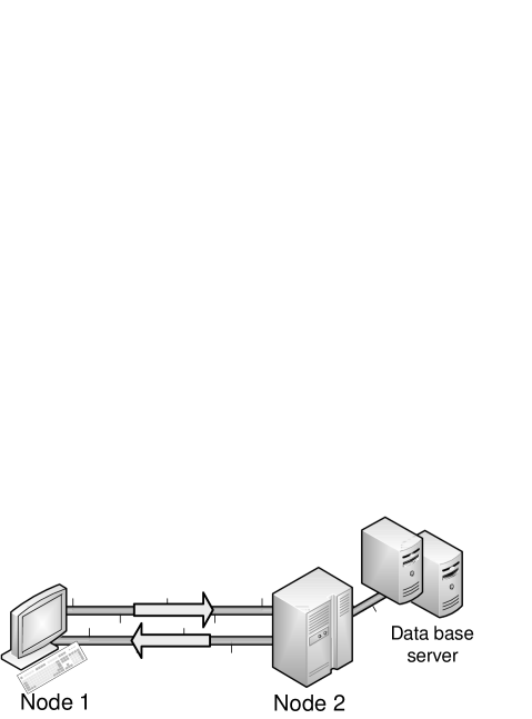
Figure 1: Two-way communication with adaptive data acquisition.

Information acquisition from the environment is generally expensive in terms of system resources, e.g., time, bandwidth or energy. For instance, accessing a remote data base requires interfacing with a server by following the appropriate protocol, and activating sensors entails some energy expenditure. Therefore, data acquisition by Node 2 should be performed efficiently by adapting to the informational requirements of Node 1 and Node 2.

To summarize the discussion above, in the system of Fig. 1 the forward communication from Node 1 to Node 2 serves three integrated purposes: i) Data exchange: Node 1 provides Node 2 with the information necessary for the latter to compute the desired quantities; ii) Query: Node 1 informs Node 2 about its own informational requirements, to be met via the backward link; iii) Control: Node 1 instructs Node 2 on the most effective way to perform data acquisition from the environment in order to satisfy Node 1’s query and to allow Node 2 to perform the desired computation.

This work sets out to analyze the setting in Fig. 1 from a fundamental theoretical standpoint via information theory. Specifically, the problem is formulated within the context of network rate-distortion theory, and the optimal communication strategy, involving the elements of data exchange, query and control, is identified. Examples are worked out to illustrate the relevance of the developed theory. Finally, the issue of robustness is tackled by assuming that, unbeknownst to Node 1, Node 2 may be unable to acquire information from the environment, due, e.g., to energy shortages or malfunctioning. The optimal robust strategy is derived and the examples extended to account for this generalized model.

I-A Related Work

The work in this paper builds on the long line of research within network information theory that deals with source coding with side information (see, e.g., [1] for an introduction). More specifically, we adopt the model of a side information “vending machine” that has been introduced in [2]. This model accounts for source coding scenarios in which acquiring information at the receiver entails some cost and thus should be done efficiently. Specifically, in this model, the quality of the side information $Y$ can be controlled at the decoder by selecting an action $A$ that affects the effective channel between the source $X$ and the side information $Y$ through a conditional distribution $p_{Y|X,A}(y|x,a)$. The distribution $p_{Y|X,A}(y|x,a)$ defines the side information “vending machine” as per the nomenclature of [2]. Each action $A$ is associated with a cost, and the problem is that of characterizing the available trade-offs among rate, distortion and action cost. We emphasize the conventional formulation of the source coding problem with side information instead assumes that the relationship between source and side information is determined by a given conditional distribution $p_{Y|X}(y|x)$ that cannot be controlled.

Various works have extended the results in [2]. Extensions to multi-terminal models can be found in [3]. Specifically, references [3]-[9] considered a set-up analogous to the Heegard-Berger problem [10, 11], in which the side information may or may not be available at the decoder. In [5], a distributed source coding setting that generalizes [12] to the case of a decoder with a side information “vending machine” is investigated. Multi-hop models were studied in [5][6].

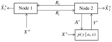
Figure 2: Two-way source coding with a side information vending machine at Node 2.

In [7], a related problem is considered in which the sequence to be compressed is dependent on the actions taken by a separate encoder. Other extensions include [8, 9] where the model of [2] is revisited under the additional constraints of common reconstruction [13] or of secrecy with respect to an "eavesdropping" node.

In this paper, the model of a side information “vending machine” is used to model the information acquisition process at Node 2 in Fig. 1. Unlike [2] and the previous work discussed above, communication between Node 1 and Node 2 is assumed to be bidirectional. The problem of characterizing the rate-distortion region for a two-way source coding models, with conventional action-independent side information sequences at Node 2 has been addressed in [14, 15, 18] and references therein.

I-B Contributions and Organization of the Paper

This work studies the model in Fig. 1, which is detailed in terms of a block diagram in Fig. 2. The system model is introduced in Sec. II. The optimal trade-off between the rates of the bidirectional communication, the distortions of the reconstructions of the desired quantities at the two nodes, and the budget for information acquisition at Node 2 is derived in Sec. III. An example that illustrates the application of the developed theory is discussed in Sec. IV. Finally, in Sec. V, the results are extended to the scenario in Fig. 5 in which, unbeknownst to Node 1, Node 2 may be unable to perform information acquisition.

Notation: Throughout the paper, a random variable is denoted by an upper case letter (e.g., $X,Y,Z$) and its realization is denoted by a lower case letter (e.g., $x,y,z$). Moreover, the shorthand notation $X^{n}$ is used to denote the tuple (or the column vector) of random variables $(X_{1},\ldots,X_{n})$, and $x^{n}$ is used to denote a realization. We define $[a,b]=[a,a+1,...,b]$ for $a\leq b$ and $[a,b]=\emptyset$, otherwise. We say that $X\textrm{---}Y\textrm{---}Z$ forms a Markov chain if $p(x,y,z)=p(x)p(y|x)p(z|y)$, that is, if $X$ and $Z$ are conditionally independent of each other given $Y$.

II System Model

The two-way source coding problem of interest, sketched in Fig. 2, is formally defined by the probability mass functions (pmfs) $p_{X}(x)$ and $p_{Y|AX}(y|a,x)$, and by the discrete alphabets $\mathcal{X},\mathcal{Y},\mathcal{A},\mathcal{\hat{X}}_{1},\mathcal{\hat{X}}_{2},$ along with distortion and cost metrics to be discussed below. The source sequence $X^{n}=(X_{1},...,X_{n})\in\mathcal{X}^{n}$ consists of $n$ independent and identically distributed (i.i.d.) entries $X_{i}$ for $i\in[1,n]$ with pmf $p_{X}(x)$. Node 1 measures sequence $X^{n}$ and encodes it in a message $M_{1}$ of $nR_{1}$ bits, which is delivered to Node 2. Node 2 wishes to estimate a sequence $\hat{X}_{2}^{n}\in\mathcal{\hat{X}}_{2}^{n}$ within given distortion requirements. To this end, Node 2 receives message $M_{1}$ and based on this, it selects an action sequence $A^{n},$ where $A^{n}\in\mathcal{A}^{n}.$

The action sequence affects the quality of the measurement $Y^{n}$ of sequence $X^{n}$ obtained at the Node 2. Specifically, given $A^{n}$ and $X^{n}$, the sequence $Y^{n}$ is distributed as $p(y^{n}|a^{n},x^{n})=\prod_{i=1}^{n}p_{Y|A,X}(y_{i}|a_{i},x_{i})$. The cost of the action sequence is defined by a cost function $\Lambda$: $\mathcal{A\rightarrow}[0,\Lambda_{\max}]$ with $0\leq\Lambda_{\max}<\infty,$ as $\Lambda(a^{n})=\sum_{i=1}^{n}\Lambda(a_{i})$. The estimated sequence $\hat{X}_{2}^{n}$ with $\hat{X}_{2}^{n}\in\mathcal{\hat{X}}_{2}^{n}$ is then obtained as a function of $M_{1}$ and $Y^{n}$.

Upon reception on the forward link, Node 2 maps the message $M_{1}$ received from Node 1 and the locally available sequence $Y^{n}$ in a message $M_{2}$ of $nR_{2}$ bits, which is delivered back to Node 1. Node 1 estimates a sequence $\hat{X}_{1}^{n}\in\mathcal{\hat{X}}_{1}^{n}$ as a function of $M_{2}$ and $X^{n}$ within given distortion requirements.

The quality of the estimated sequence $\hat{X}_{j}^{n}$ is assessed in terms of the distortion metrics $d_{j}(x,y,\hat{x}_{j})$: $\mathcal{X}\times\mathcal{Y}\times\mathcal{\hat{X}}_{j}\rightarrow\mathbb{R_{+}}\cup\{\infty\}$ for $j=1,2,$ respectively. Note that this implies that $\hat{X}_{j}^{n}$ is allowed to be a lossy version of any function of the source and side information sequences. A more general model is studied in Sec. III-A. It is assumed that $D_{j}=\min_{\hat{x}_{j}\in\hat{\mathcal{X}}_{j}}E[d(X,Y,\hat{X}_{j})]<\infty$ for $j=1,2$. A formal description of the operations at encoder and decoder follows.

Definition 1.

An $(n,R_{1},R_{2},D_{1},D_{2},\Gamma,\epsilon)$ code for the set-up of Fig. 2 consists of a source encoder for Node 1

$$\mathrm{g}_{1}\text{: }\mathcal{X}^{n}\rightarrow[1,2^{nR_{1}}],$$ (1)

which maps the sequence $X^{n}$ into a message $M_{1};$ an “action” function

$$\mathrm{\ell}\text{: }[1,2^{nR_{1}}]\times\mathcal{Y}^{i-1}\rightarrow\mathcal{A},$$ (2)

which maps the message $M_{1}$ and the previously observed into an action sequence $A^{n};$ a source encoder for Node 2

$$\mathrm{g}_{2}\text{:}\text{ }\mathcal{Y}^{n}\times[1,2^{nR_{1}}]\rightarrow[1,2^{nR_{2}}],$$ (3)

which maps the sequence $Y^{n}$ and message $M_{1}$ into a message $M_{2};$ two decoders, namely

$$\mathrm{h}_{1}\text{: }[1,2^{nR_{2}}]\times\mathcal{X}^{n}\rightarrow\mathcal{\hat{X}}_{1}^{n},$$ (4)

which maps the message $M_{2}$ and the sequence $X^{n}$ into the estimated sequence $\hat{X}_{1}^{n};$

$$\mathrm{h}_{2}\text{: }[1,2^{nR_{1}}]\times\mathcal{Y}^{n}\rightarrow\mathcal{\hat{X}}_{2}^{n},$$ (5)

which maps the message $M_{1}$ and the sequence $Y^{n}$ into the estimated sequence $\hat{X}_{2}^{n};$ such that the action cost constraint $\Gamma$ and distortion constraints $D_{j}$ for $j=1,2$ are satisfied, i.e.,

$$\frac{1}{n}\underset{i=1}{\overset{n}{\sum}}\mathrm{E}\left[\Lambda(A_{i})\right] \leq\Gamma$$ (6)

$$\text{ and }\frac{1}{n}\underset{i=1}{\overset{n}{\sum}}\mathrm{E}\left[d_{j}(X_{i},Y_{i},\hat{X}_{ji})\right] \leq D_{j}\text{ for }j=1,2.$$ (7)

Definition 2.

Given a distortion-cost tuple $(D_{1},D_{2},\Gamma)$, a rate tuple $(R_{1},R_{2})$ is said to be achievable if, for any $\epsilon>0$, and sufficiently large $n$, there exists a $(n,R_{1},R_{2},D_{1}+\epsilon,D_{2}+\epsilon,\Gamma+\epsilon)$ code.

Definition 3.

The rate-distortion-cost region $\mathcal{R}(D_{1},D_{2},\Gamma)$ is defined as the closure of all rate tuples $(R_{1},R_{2})$ that are achievable given the distortion-cost tuple $(D_{1},D_{2},\Gamma)$.

Remark 4.

For the special case in which the side information $Y$ independent of the action $A$ given $X$, i.e., for $\ p(y|a,x)=p(y|x),$ the rate-distortion region $\mathcal{R}(D_{1},D_{2},\Gamma)$ has been derived in [14]. Instead, if $D_{2}=D_{2,max}$, the set of all achievable rates $R_{1}$ was characterized in [2].

Remark 5.

The definition (2) of an action encoder allows for adaptation of the actions to the previously observed values of the side information $Y$. This possibility was studied in [16] for the point-to-point one-way model, which is obtained by setting $R_{2}=0$ in the setting of Fig. 2.

In the following sections, for simplicity of notation, we drop the subscripts from the definition of the pmfs, thus identifying a pmf by its argument.

III Rate-Distortion-Cost Region

In this section, a single-letter characterization of the rate-distortion-cost region is derived.

Proposition 6.

The rate-distortion-cost region $\mathcal{R\mbox{$(D_{1},D_{2},\Gamma)$}}$ for the two-way source coding problem illustrated in Fig. 2 is given by the union of all rate pairs $(R_{1},R_{2})$ that satisfy the conditions

$$R_{1} \geq I(X;A)+I(X;U|A,Y)$$ (8a)

$$\ce{and}\mbox{ }R_{2} \geq I(Y;V|A,X,U),$$ (8b)

where the mutual information terms are evaluated with respect to the joint pmf

$$p(x,y,a,u,v)=p(x)p(a,u|x)p(y|a,x)p(v|a,u,y)$$ , (9)

for some pmfs $p(a,u|x)$ and $p(v|a,u,y)$ such that the inequalities

$$\ce{E}[d_{1}(X,Y,\ce{f}_{1}(V,X))] \leq D_{1},$$ (10a)

$$\ce{E}[d_{2}(X,Y,\ce{f}_{2}(U,Y))] \leq D_{2},$$ (10b)

$$\ce{and}\textrm{ }\ce{E}[\Lambda(A)] \leq \Gamma,$$ (10c)

are satisfied for some function $\ce{f}_{1}\textrm{: }\mathcal{V}\times\mathcal{X}\rightarrow\hat{\mathcal{X}}_{1}$ and $\ce{f}_{2}\textrm{: }\mathcal{U}\times\mathcal{Y}\rightarrow\hat{\mathcal{X}}_{2}$. Finally, $U$ and $V$ are auxiliary random variables whose alphabet cardinality can be constrained as $|\mathcal{U}|\leq|\mathcal{X}||\mathcal{A}|+4$ and $|\mathcal{V}|\leq|\mathcal{U}||\mathcal{Y}||\mathcal{A}|+1$ without loss of optimality.

Remark 7.

For the special case in which the side information $Y$ is independent of the action $A$ given $X$, i.e., for $p(y|a,x)=p(y|x),$ the rate-distortion region $\mathcal{R}(D_{1},D_{2},\Gamma)$ in Proposition 6 reduces to that derived in [14, 15]. Instead, if $D_{2}=D_{2,max}$, the result reduces to that in [2].

The proof of the converse is provided in Appendix A. The achievability follows as a combination of the techniques proposed in [2] and [14], and requires the forward link to be used, in an integrated manner, for data exchange, query and control. Specifically, for the forward link, similar to [2], Node 1 uses a successive refinement codebook. Accordingly, the base layer is used by Node 1 to instruct Node 2 on which actions are best tailored to fulfill the informational requirements of both Node 1 and Node 2. This base layer thus represents control information that also serves the purpose of querying Node 2 in view of the backward communication. We observe that Node 1 selects this base layer as a function of the source $X^{n}$, thus allowing Node 2 to adapt its actions for information acquisition to the current realization of the source $X^{n}$. The refinement layer of the code used by Node 1 is leveraged, instead, to provide additional information to Node 2 in order to meet Node 2’s distortion requirement. Node 2 then employs standard Wyner-Ziv coding (i.e., binning) [1] for the backward link to satisfy Node 1’s distortion requirement.

We now briefly outline the main technical aspects of the achievability proof, since the details follow from standard arguments and do not require further elaboration here. To be more precise, Node 1 first maps sequence $X^{n}$ into the action sequence $A^{n}$ using the standard joint typicality criterion. This mapping requires a codebook of rate $I(X;A)$ (see, e.g., [1, pp. 62-63]). Given the sequence $A^{n}$, the description of sequence $X^{n}$ is further refined through mapping to a sequence $U^{n}$. This requires a codebook of size $I(X;U|A,Y)$ for each action sequence $A^{n}$ using Wyner-Ziv binning with respect to side information $Y^{n}$ [1, pp. 62-63]. In the reverse link, Node 2 employs Wyner-Ziv coding for the sequence $Y^{n}$ by leveraging the side information $X^{n}$ available at Node 1 and conditioned on the sequences $U^{n}$ and $A^{n}$, which are known to both Node 1 and Node 2 as a result of the communication on the forward link. This requires a rate equal to the right-hand side of (8b). Finally, Node 1 and Node 2 produce the estimates $\hat{X}_{1}^{n}$ and $\hat{X}_{2}^{n}$ as the symbol-by-symbol functions $\hat{X}_{1i}=\textrm{f}_{1}(V_{i},X_{i})$ and $\hat{X}_{2i}=\textrm{f}_{2}(U_{i},Y_{i})$ for $i\in[1,n]$, respectively.

Remark 8.

The achievability scheme discussed above uses actions that do not adapt to the previous values of the side information $Y$. The fact that this scheme attains the optimal performance characterized in Proposition 6 shows that, as demonstrated in [16] for the one-way model with $R_{2}=0$, adaptive actions do not improve the rate-distortion performance.

III-A Indirect Rate-Distortion-Cost Region

In this section, we consider a more general model in which Node 1 observes only a noisy version of the source $X^{n}$, as depicted in Fig. 3. Following [17], we refer to this setting as posing an indirect source coding problem. The example studied in Sec. IV illustrates the relevance of this generalization. The system model is as defined in Sec. II with the following differences. The source encoder for Node 1

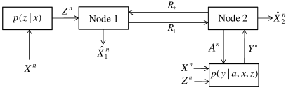
Figure 3: Indirect two-way source coding with a side information vending machine at Node 2.

$$\mathrm{g}_{1}\text{: }\mathcal{Z}^{n}\rightarrow[1,2^{nR_{1}}],$$ (11)

maps the sequence $Z^{n}$ into a message $M_{1};$ the decoder for Node 1

$$\mathrm{h}_{1}\text{: }[1,2^{nR_{2}}]\times\mathcal{Z}^{n}\rightarrow\mathcal{\hat{X}}_{1}^{n},$$ (12)

maps the message $M_{2}$ and the sequence $Z^{n}$ into the estimated sequence $\hat{X}_{1}^{n};$ given $(X^{n},A^{n},Z^{n})$, the side information $Y^{n}$ is distributed as $p(y^{n}|a^{n},x^{n},z^{n})=\prod_{i=1}^{n}p_{Y|A,X,Z}(y_{i}|a_{i},x_{i},z_{i})$ and the distortion constraints are given as

$$\frac{1}{n}\underset{i=1}{\overset{n}{\sum}}\mathrm{E}\left[d_{j}(X_{i},Y_{i},Z_{i},\hat{X}_{ji})\right] \leq D_{j}\text{ for }j=1,2,$$ (13)

for some distortion metrics $d_{j}(x,y,z,\hat{x}_{j}):$$\mathcal{X}\times\mathcal{Y}\times{\cal Z}\times\mathcal{\hat{X}}_{j}\rightarrow\mathbb{R_{+}}\cup\{\infty\}$, for $j=1,2$. The next proposition derives a single-letter characterization of the rate-distortion-cost region.

Proposition 9.

The rate-distortion-cost region $\mathcal{R\mbox{$(D_{1},D_{2},\Gamma)$}}$ for the indirect two-way source coding problem illustrated in Fig. 3 is given by the union of all rate pairs $(R_{1},R_{2})$ that satisfy the conditions

$$R_{1} \geq I(Z;A)+I(Z;U|A,Y)$$ (14a)

$$\ce{and}\mbox{ }R_{2} \geq I(Y;V|A,Z,U),$$ (14b)

where the mutual information terms are evaluated with respect to the joint pmf

$$p(x,y,z,a,u,v)\negmedspace=\negmedspace p(x,z)p(a,\negmedspace u|z)p(y|a,\negmedspace x,\negmedspace z)p(v|a,\negmedspace u,\negmedspace y),$$ (15)

for some pmfs $p(a,u|x)$ and $p(v|a,u,y)$ such that the inequalities

$$\ce{E}[d_{1}(X,Y,Z,\ce{f}_{1}(V,Z))] \leq D_{1},$$ (16a)

$$\ce{E}[d_{2}(X,Y,Z,\ce{f}_{2}(U,Y))] \leq D_{2},$$ (16b)

$$\ce{and}\textrm{ }\ce{E}[\Lambda(A)] \leq \Gamma,$$ (16c)

are satisfied for some function $\ce{f}_{1}\textrm{: }\mathcal{V}\times\mathcal{Z}\rightarrow\hat{\mathcal{X}}_{1}$ and $\ce{f}_{2}\textrm{: }\mathcal{U}\times\mathcal{Y}\rightarrow\hat{\mathcal{X}}_{2}$. Finally, $U$ and $V$ are auxiliary random variables whose alphabet cardinality can be constrained as $|\mathcal{U}|\leq|\mathcal{Z}||\mathcal{A}|+3$ and $|\mathcal{V}|\leq|\mathcal{U}||\mathcal{Y}||\mathcal{A}|+1$ without loss of optimality.

The proof of the achievability and converse follows with slight modifications from that of Proposition 6. Specifically, in the achievability the sequence $X^{n}$ is replaced by its noisy version, i.e., the sequence $Z^{n}$, and the rest of the proof remains essentially unchanged. The proof of the converse is provided in Appendix A.

IV Example

In this section, we consider a binary example for the set-up in Fig. 3 to illustrate the main aspects of the problem and the relevance of the theoretical results derived above. Specifically, we assume binary alphabets as ${\cal X}={\cal A}=\{0,1\}$ and a source distribution $X\sim\textrm{Bern}(0.5)$. Moreover, the source $Z^{n}$ measured by Node 1 is an erased version of the source $X^{n}$ with erasure probability $\epsilon$. This means that $Z_{i}=\textrm{e}$, where e represents an erasure, with probability $\epsilon$ and $Z_{i}=X_{i}$ with probability $1-\epsilon$, for $i\in[1,n]$.

The vending machine at Node 2 operates as follows:

$$Y = \left\{\begin{array}[]{lc}X&\mbox{ for }A=1\\ \phi&\textrm{\mbox{ for }}A=0\end{array},\right.$$ (19)

with cost constraint $\Lambda(a)=a$, for $a\in\{0,1\},$ where $\phi$ is a dummy symbol representing the case in which no useful information is acquired by Node 2. This model implies that a cost budget of $\Gamma$ limits the average number of samples of the sequence $Y$ that can be measured by Node 2 to around $n\Gamma$ given the constraint (6).

Node 1 wishes to reconstruct a lossy version of the source $X^{n}$, while Node 2 is interested in $Z^{n}$. The distortion functions are the Hamming metrics $d_{1}(x,\hat{x}_{1})=1_{\{x\neq\hat{x}_{1}\}}$ and $d_{2}(z,\hat{x}_{2})=1_{\{z\neq\hat{x}_{2}\}}$. To obtain analytical insight into the rate-distortion-cost region, in the following we focus on a number of special cases.

IV-A $D_{1}=D_{1,max}$ and $D_{2}=0$

Consider the distortion requirements $D_{1}=D_{1,max}$ and $D_{2}=0$. As a result, Node 1 requires no backward communication from Node 2, while Node 2 wishes to recover $Z^{n}$ losslessly. For the given distortions, the rate-cost region in Proposition 9 can be evaluated as

$$R_{1} \geq H_{2}(\epsilon)+(1-\epsilon-\Gamma)^{+}$$ (20a)

$$\ce{and}\mbox{ }R_{2} \geq 0,$$ (20b)

for any cost budget $\Gamma\geq 0$, where $H_{2}(\alpha)=-\alpha\ce{log_{2}}\alpha-(1-\alpha)\ce{log_{2}}(1-\alpha)$ is the binary entropy function.

A formal proof of this result can be found in Appendix B. The rate region (20) shows that, as the cost budget $\Gamma$ for information acquisition increases, the required rate $R_{1}$ decreases down to the rate $H_{2}(\epsilon)$ that is required to describe only the erasures process $E^{n}$ with $E_{i}=1_{\{Z_{i}=\ce{e}\}}$, $i=1,...,n$, losslessly to Node 2. This can be explained by noting that the following time-sharing strategy achieves region (20) and is thus optimal.

Node 1 describes the process $E^{n}$ losslessly to Node 2 with $H_{2}(\epsilon)$ bits per symbol. In order to obtain a lossless reconstruction of $Z^{n}$, Node 2 needs to be informed about $Z_{i}=X_{i}$ for all $i$ in which $E_{i}=0$. This information can be interpreted as control data that is used by Node 2 to adapt its information acquisition process. Note that we have around $n(1-\epsilon)$ such samples of $Z_{i}$. Node 1 describes $Z_{i}=X_{i}$ for $n(1-\epsilon-\Gamma)^{+}$ of these samples, while the remaining $n\ce{min}(\Gamma,1-\epsilon)$ are measured by Node 2 through the vending machine. An alternative strategy based directly on Proposition 9 can be found in Appendix B.

Fig. 4 illustrates the rate $R_{1}$ in (20a) versus the cost budget $\Gamma$ for $\epsilon=0.2$. We observe that if $\Gamma\geq 1-\epsilon=0.8$ no further improvement of the rate is possible as per (20a).

IV-B $D_{1}=0$ and $D_{2}=D_{2,max}$

Here we consider the dual case in which Node 1 wishes to reconstruct sequence $X^{n}$ losslessly ($D_{1}=0$), while Node 2 does not have any distortion requirements ($D_{2}=D_{2,max}$). As shown in Appendix B, if $\Gamma\geq\epsilon$, the rate-cost region is given by the union of all rate pairs $(R_{1},R_{2})$ such that

$$R_{1} \geq H_{2}(\epsilon)-\Gamma H\Bigl{(}\frac{\epsilon}{\Gamma}\Bigr{)}$$ (21a)

$$\ce{and}\mbox{ }R_{2} \geq \epsilon.$$ (21b)

Moreover, for $\Gamma<\epsilon$, the region is empty as the lossless reconstruction of $X$ at Node 1 is not feasible.

A proof of this result based on Proposition 9 can be found in Appendix B. In the following, we argue that a natural time-sharing strategy, akin to that used for the case $D_{1}=D_{1,max},\textrm{}D_{2}=0$ above, would be suboptimal, implying that the optimal strategy requires a more sophisticated approach based on the successive refinement code presented in Sec. III.

A natural time-sharing strategy would be the following. Node 1 describes $n\eta$ samples of the erasure process $E^{n}$, for some $0\leq\eta\leq 1$, losslessly to Node 2, using rate $R_{1}=\eta H_{2}(\epsilon)$. This information is used by Node 1 to query Node 2 about the desired information. Specifically, Node 2 sets $A_{i}=1$ if $E_{i}=1$, thus observing around $n\eta\epsilon$ samples $Y_{i}=X_{i}$ from the vending machine. These samples are needed to fulfill the distortion requirements of Node 1. For all the remaining $n(1-\eta$) samples, for which Node 2 does not have control information from Node 1, Node 2 sets $A_{i}=1$, thus acquiring all the side information samples. Again, this is necessary given Node 1’s requirements. Node 2 conveys losslessly the $n\eta\epsilon$ samples $Y_{i}=X_{i}$ obtained when $E_{i}=1$, which requires $\eta\epsilon$ bits per sample, along with the $n(1-\eta)$ samples $Y_{i}$ in the second set, which amount instead to $(1-\eta)H(X|Z)$ bits per sample. Note that we have the rate $H(X|Z)$ by the Slepian-Wolf theorem [1, Chapter 10], since Node 1 has side information $Z_{i}$ for the second set of samples. Overall, we have $R_{2}=\eta\epsilon+(1-\eta)\epsilon=\epsilon$ bits/source symbol. This entails a cost budget of $\Gamma=\eta\epsilon+1-\eta$, and thus $\eta=\nicefrac{{(1-\Gamma)}}{{(1-\epsilon)}}$.

Fig. 4 compares the rate $R_{1}$ as in (21a) with the corresponding rate obtained via time-sharing, for $\epsilon=0.2$. As seen, in this second case the time-sharing strategy is strictly suboptimal.

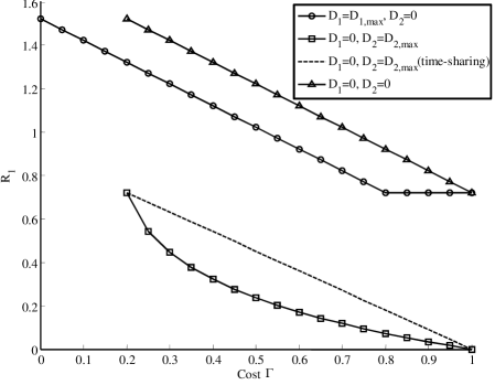
Figure 4: Rate $R_{1}$ versus cost $\Gamma$ for the examples in Sec. IV with $\epsilon=0.2$.

IV-C $D_{1}=D_{2}=0$

We now consider the case in which both nodes wish to achieve lossless reconstruction, i.e., $D_{1}=D_{2}=0$. As seen in the previous case, achieving $D_{1}=0$ is not possible if $\Gamma<\epsilon$ and thus this is a fortiori true for $D_{1}=D_{2}=0$. For $\Gamma\geq\epsilon$, the rate-cost region is given by

$$R_{1} \geq H_{2}(\epsilon)+(1-\Gamma)$$ (22a)

$$\ce{and}\mbox{ }R_{2} \geq \epsilon,$$ (22b)

as shown in Appendix B.

A time-sharing strategy that achieves (22) is as follows. Node 1 describes the process $E^{n}$ losslessly to Node 2 with $H_{2}(\epsilon)$ bits per symbol. This information serves the functions of query and control for Node 2. In order to satisfy its distortion requirement, Node 2 now needs to be informed about $Z_{i}=X_{i}$ for all $i$ in which $E_{i}=0$. Note that we have $n(1-\epsilon)$ such samples of $Z_{i}$. Node 1 describes $Z_{i}=X_{i}$ for $n(1-\Gamma)\leq n(1-\epsilon)$ of these samples, while the remaining $n(\Gamma-\epsilon)$ are measured by Node 2 through the vending machine. Node 2 compresses losslessly the sequence of around $n\epsilon$ samples of $X_{i}$ with $i$ such that $E_{i}=1$ which requires $R_{2}=\epsilon$ bits per sample.

Fig. 4 illustrates the rate $R_{1}$ in (22a) versus the cost budget $\Gamma$ for $\epsilon=0.2$.

V When the Side Information May Be Absent

In this section, we generalize the results of the previous section to the scenario in Fig. 5 in which, unbeknownst to Node 1, Node 2 may be unable to perform information acquisition due, e.g., to energy shortage or malfunctioning. This set-up is illustrated in Fig. 5.

V-A System Model

The formal description of an $(n,R_{1},R_{2},D_{1},D_{2},D_{3},\Gamma,\epsilon)$ code for the set-up of Fig. 5 is given as in Sec. III-A (which generalizes the model in Sec. II) with the addition of Node 3. This added node, which has no access to the side information, models the situation in which the recipient of the communication from Node 1 happens to be unable to acquire information from the environment. Note that the same message $M_{1}$ from Node 1 is received by both Node 2 and Node 3. This captures the fact that the information about whether or not the recipient is able to access the side information is not available to Node 1. The model in Fig. 5 is a generalization of the so called Heegard-Berger problem [10, 11].

Formally, Node 3 is defined by the decoding function

$$\mathrm{h}_{3}\text{: }[1,2^{nR_{1}}]\rightarrow\mathcal{\hat{X}}_{3}^{n},$$ (23)

which maps the message $M_{1}$ into the the estimated sequence $\hat{X}_{3}^{n};$ and the additional distortion constraint

$$\frac{1}{n}\underset{i=1}{\overset{n}{\sum}}\mathrm{E}\left[d_{3}(X_{i},Y_{i},Z_{i},\hat{X}_{3i})\right] \leq D_{3}.$$ (24)

We remark that adding a link between Node 3 and Node 1 cannot improve the system performance given that Node 3 has only available the message $M_{1}$ received from Node 1. Therefore, this link is not included in the model.

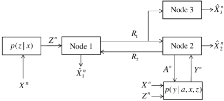
Figure 5: Indirect two-way source coding when the side information vending machine may be absent at the recipient of the message from Node 1.

V-B Rate-Distortion-Cost Region

In this section, a single-letter characterization of the rate-distortion-cost region is derived for the set-up in Fig. 5.

Proposition 10.

The rate-distortion-cost region $\mathcal{R\mbox{$(D_{1},D_{2},D_{3},\Gamma)$}}$ for the two-way source coding problem illustrated in Fig. 5 is given by the union of all rate pairs $(R_{1},R_{2})$ that satisfy the conditions

$$R_{1} \negmedspace\geq\negmedspace I(Z;A)+I(Z;\hat{X}_{3}|A)$$ (25a)

$$+I(Z;U|A,Y,\hat{X}_{3})$$

$$\ce{and}\mbox{ }R_{2} \negmedspace\geq\negmedspace I(Y;V|A,Z,U,\hat{X}_{3}),$$ (25b)

where the mutual information terms are evaluated with respect to the joint pmf

$$p(x,y,z,a,u,v)= p(x,z)p(a,u,\hat{x}_{3}|z)p(y|a,x,z)$$

$$p(v|a,u,y,\hat{x}_{3}),$$ (26)

for some pmfs $p(a,u,\hat{x}_{3}|z)$ and $p(v|a,u,y)$ such that the inequalities

$$\ce{E}[d_{1}(X,Y,Z,\ce{f}_{1}(V,Z))] \leq D_{1},$$ (27a)

$$\ce{E}[d_{2}(X,Y,Z,\ce{f}_{2}(U,Y))] \leq D_{2},$$ (27b)

$$\ce{E}[d_{3}(X,Y,Z,\hat{X}_{3})] \leq D_{3},$$ (27c)

$$\ce{and}\textrm{ }\ce{E}[\Lambda(A)] \leq \Gamma,$$ (27d)

are satisfied for some function $\ce{f}_{1}\textrm{: }\mathcal{V}\times\mathcal{Z}\rightarrow\hat{\mathcal{X}}_{1}$ and $\ce{f}_{2}\textrm{: }\mathcal{U}\times\mathcal{Y}\rightarrow\hat{\mathcal{X}}_{2}$. Finally, $U$ and $V$ are auxiliary random variables whose alphabet cardinality can be constrained as $|\mathcal{U}|\leq|\mathcal{Z}||\mathcal{A}|+3$ and $|\mathcal{V}|\leq|\mathcal{U}||\mathcal{Y}||\mathcal{A}|+1$ without loss of optimality.

The proof of the converse is provided in Appendix A. The achievable rate (25a) can be interpreted as follows. Node 1 uses a successive refinement code with three layers. The first layer is defined as for Sec. III and carries query and control information. The second and third layers are designed as in the optimal Heegard-Berger scheme [10]. Specifically, the second layer is destined to both Node 2 and Node 3, while the third layer targets only Node 2, which has enhanced decoding capabilities due to the availability of side information.

To provide further details, as for Proposition 6, the encoder first maps the input sequence $Z^{n}$ into an action sequence $A^{n}$ so that the two sequences are jointly typical, which requires $I(Z;A)$ bits/source sample. Then, it maps $Z^{n}$ into the estimate $\hat{X}_{3}^{n}$ for Node 3 using a conditional codebook with rate $I(Z;\hat{X}_{3}|A)$. Finally, it maps $Z^{n}$ into another sequence $U^{n}$ using the fact that Node 2 has the action sequence $A^{n}$, the estimate $\hat{X}_{3}^{n}$ and the measurement $Y^{n}$. Using conditional codebooks (with respect to $\hat{X}_{3}^{n}$ and $A^{n}$) and from the Wyner-Ziv theorem, this requires $I(Z;U|A,Y,\hat{X}_{3})$ bit/source sample. As for the rate (25b), Node 2 employs Wyner-Ziv coding for the sequence $Y^{n}$ by leveraging the side information $Z^{n}$ available at Node 1 and conditioned on the sequences $U^{n}$, $A^{n}$ and $\hat{X}_{3}^{n}$, which are known to both Node 1 and Node 2 as a result of the forward communication. This requires a rate equal to the right-hand side of (25b). Finally, Node 1 and Node 2 produce the estimates $\hat{X}_{1}^{n}$ and $\hat{X}_{2}^{n}$ as the symbol-by-symbol functions $\hat{X}_{1i}=\textrm{f}_{1}(V_{i},Z_{i})$ and $\hat{X}_{2i}=\textrm{f}_{2}(U_{i},Y_{i})$ for $i\in[1,n]$, respectively.

V-C Example

In this section, we extend the binary example of Sec. IV to the set-up in Fig. 5. Specifically, we consider the same setting as in Sec. IV, with the addition of Node 3. For the latter, we assume a ternary reconstruction alphabet ${\cal\hat{X}}_{3}=\{0,1,*\}$ and the distortion metric $d_{3}(x,z,\hat{x}_{3})=d_{3}(\mathbf{1}_{\{Z=\ce{e}\}},\hat{x}_{3})$ in Table I, where we recall that $E_{i}=\mathbf{1}_{\{Z_{i}=\ce{e}\}}$ is the erasure process. Accordingly, Node 3 is interested in recovering the erasure process $E^{n}$ under an erasure distortion metric (see, e.g., [19]) , where “*” represents the “don’t care” or erasure reproduction symbol

Table I: Erasure distortion for reconstruction at Node 3.

We first observe that for cases 1) and 3) in Sec. IV the distortion requirements of Node 3 do not change the rate-distortion function. This is because, as discussed in Sec. IV, the requirement that $D_{2}$ be equal to zero entails that the erasure process $E^{n}$ be communicated losslessly to Node 2 without leveraging the side information from the vending machine (which cannot provide information about the erasure process). It follows that one can achieve $D_{3}=0$ at no additional rate cost. We thus now focus on the case 2) in Sec. IV, namely $D_{1}=0$ and $D_{2}=D_{2,max}$.

In the case at hand, Node 1 wishes to recover $X^{n}$ losslessly, Node 2 has no distortion requirements and Node 3 wants to recover $E^{n}$ with distortion $D_{3}$. As explained in Sec. IV-B, in order to reconstruct $X^{n}$ losslessly at Node 1 we must have $\Gamma\geq\epsilon$ and $\ce{Pr}(A=1|Z=\ce{e})=1$. Moreover, due to symmerty of the problem with respect to $Z=0$ and $Z=1$, we can set $\ce{Pr}(A=1|Z=0)=\ce{Pr}(A=1|Z=1)=\frac{\gamma-\epsilon}{1-\epsilon}$, for some $0\leq\gamma\leq\Gamma$. To evaluate the rate-distortion-cost region (25), we then define $\ce{Pr}(\hat{X}_{3}=*|A=1,Z=\ce{e})\overset{\triangle}{=}p_{1}$, $\ce{Pr}(\hat{X}_{3}=*|A=0,Z=0)\overset{\triangle}{=}p_{2}$ and $\ce{Pr}(\hat{X}_{3}=*|A=1,Z=0)\overset{\triangle}{=}p_{3}$. We thus get that the rate-distortion-cost region is given by

$$R_{1} \geq H_{2}(\epsilon)+1-\epsilon-(1-\Gamma)(1-p_{2})-(\Gamma-\epsilon)$$

$$(1-p_{3})-(1-\Gamma)p_{2}-\Bigl{(}\epsilon p_{1}+(\Gamma-\epsilon)p_{3}\Bigr{)}$$

$$\Bigl{(}H_{2}(\frac{\epsilon p_{1}}{\epsilon p_{1}+(\Gamma-\epsilon)p_{3}})+\frac{(\Gamma-\epsilon)p_{3}}{\epsilon p_{1}+(\Gamma-\epsilon)p_{3}}\Bigr{)}$$ (28a)

$$\ce{and}\mbox{ }R_{2} \geq\epsilon,$$ (28b)

where parameters $p_{1},p_{2},p_{3}\in[0,1]$ must be selected so as to satisfy the distortion constraint of Node 3, namely $D_{3}\geq\epsilon p_{1}+(1-\Gamma)p_{2}+(\Gamma-\epsilon)p_{3}$.

Fig. 6 illustrates the rate $R_{1}$ in (28a), minimized over $p_{1},p_{2}$ and $p_{3}$ under the constraints mentioned above versus the cost budget $\Gamma$ for $\epsilon=0.2$ and different values of $D_{3}$, namely $D_{3}=0.4,$ $0.6$, $0.8$ and $D_{3}=D_{3,max}=1$. Note that for $D_{3}=D_{3,max}=1$ we obtain the rate in (21a). As it can be seen, for $\Gamma\leq D_{3}$, the rate decreases with increasing cost $\Gamma$, but for $\mbox{$\Gamma\geq$}D_{3}$ the rate remains constant while increasing $\Gamma$. The reason is that for the latter region, i.e., $\Gamma\geq D_{3}$, the performance of the system is dominated by the distortion requirement of Node 3 and thus increasing the cost budget $\Gamma$ does not improve the rate. Instead, for $\Gamma\leq D_{3}$, it is sufficient to cater only to Node 2, and Node 3 is able to recover $E$ with distortion $D_{3}=\Gamma$ at no additional rate cost.

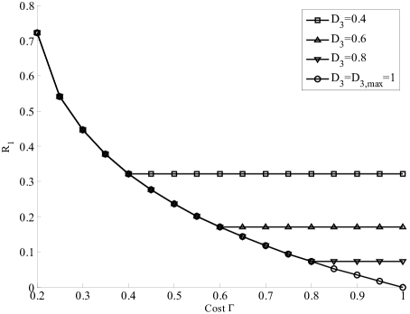
Figure 6: Rate $R_{1}$ versus cost $\Gamma$ for the examples in Sec. V-C with $\epsilon=0.2$, $D_{1}=0$ and $D_{2}=D_{2,max}$.

VI Concluding Remarks

For applications such as complex communication networks for cloud computing or machine-to-machine communication, the bits exchanged by two parties serve a number of integrated functions, including data transmission, control and query. In this work, we have considered a baseline two-way communication scenario that captures some of these aspects. The problem is addressed from a fundamental theoretical standpoint using an information theoretic formulation. The analysis reveals the structure of optimal communication strategies and can be applied to elaborate on specific examples, as illustrated in the paper. This work opens a number of possible avenues for future research, including the analysis of scenarios in which more than one round of interactive communication is possible [18].

Appendix A: Converse Proof for Proposition 6

Here, we prove the converse part of Proposition 6. For any $(n,R_{1},R_{2},D_{1}+\epsilon,D_{2}+\epsilon,\Gamma+\epsilon)$ code, we have the series of inequalities

$$nR_{1}\geq H(M_{1})$$

$$\stackrel{{\scriptstyle(a)}}{{=}}I(M_{1};X^{n},Y^{n})$$

$$=H(X^{n})+H(Y^{n}|X^{n})$$

$$-H(Y^{n}|M_{1})-H(X^{n}|Y^{n},M_{1})$$

$$\stackrel{{\scriptstyle(b)}}{{\geq}}\sum_{i=1}^{n}H(X_{i})-H(X_{i}|X_{i+1}^{n},Y^{n},M_{1},A^{i})$$

$$+H(Y_{i}|Y^{i-1},X^{n},M_{1},A_{i})-H(Y_{i}|Y^{i-1},M_{1},A_{i})$$

$$\stackrel{{\scriptstyle(c)}}{{\geq}}\negmedspace\sum_{i=1}^{n}\negmedspace H\negmedspace(X_{i})\negmedspace-\negmedspace H\negmedspace(X_{i}|A_{i},Y_{i},U_{i})\negmedspace+\negmedspace H\negmedspace(Y_{i}|X_{i},\negmedspace A_{i})\negmedspace-\negmedspace H\negmedspace(Y_{i}|A_{i}),$$ (29)

where $(a)$ follows since $M_{1}$ is a function of $X^{n}$ and since conditioning reduces entropy; $(b)$ follows since $A_{i}$ is a function of $(M_{1},Y^{i-1})$ and $M_{1}$ is a function of $X^{n}$ and $(c)$ follows since conditioning decreases entropy, by defining $U_{i}=(M_{1},X_{i+1}^{n},A^{i-1},Y^{i-1})$ and using the fact that the vending machine is memoryless. We also have the series of inequalities

$$nR_{2}\geq H(M_{2})$$

$$\geq H(M_{2}|X^{n},M_{1})$$

$$\stackrel{{\scriptstyle(a)}}{{=}}I(M_{2};Y^{n}|X^{n},M_{1})$$

$$\stackrel{{\scriptstyle(b)}}{{=}}\sum_{i=1}^{n}H(Y_{i}|Y^{i-1},X^{n},M_{1},A^{i})$$

$$-H(Y_{i}|Y^{i-1},X^{n},M_{1},M_{2},A^{i})$$

$$\stackrel{{\scriptstyle(c)}}{{\geq}}\negmedspace\sum_{i=1}^{n}\negmedspace H\negmedspace(Y_{i}|X_{i},\negmedspace A_{i},\negmedspace U_{i})\negmedspace-\negmedspace H(Y_{i}|X_{i},\negmedspace A_{i},\negmedspace U_{i},\negmedspace V_{i}),$$ (30)

where $(a)$ follows since $M_{2}$ is a function of $(M_{1},Y^{n})$, $(b)$ follows since $A_{i}$ is a function of $(M_{1},Y^{i-1})$ and $(c)$ follows since the Markov chain $Y_{i}\textrm{---}(X_{i},U_{i},A_{i})\textrm{---}X^{i-1}$ holds by the problem definition (this can be easily checked by using d-separation on the Bayesian network representation of the joint distribution of the variables at hand as induced by the system model

Figure 7: Bayesian network representing the joint pmf of variables $(M_{1},M_{2},X^{n},Y^{n},A^{n})$ for the two-way source coding problem with a vending machine in Fig. 2.

in Fig. 7, see, e.g., [20, Sec. A.9]), since conditioning reduces entropy and by defining $V_{i}=M_{2}$.

Defining $Q$ to be a random variable uniformly distributed over $[1,n]$ and independent of all the other random variables and with $X\overset{\triangle}{=}X_{Q}$, $Y\overset{\triangle}{=}Y_{Q}$, $A\overset{\triangle}{=}A_{Q}$, $\hat{X}_{1}\overset{\triangle}{=}\hat{X}_{1Q}$, $\hat{X}_{2}\overset{\triangle}{=}\hat{X}_{2Q}$, $V\overset{\triangle}{=}(V_{Q},Q)$ and $U\overset{\triangle}{=}(U_{Q},Q),$ from (29) we have

$$nR_{1} \geq H(X|Q)-H(X|A,Y,U,Q)$$ (31)

$$+H(Y|X,A,Q)-H(Y|A,Q)$$

$$\stackrel{{\scriptstyle(a)}}{{\geq}} H(X)-H(X|A,Y,U)$$

$$+H(Y|X,A)-H(Y|A)$$

$$= I(X;A)+I(X;U|A,Y),$$

where $(a)$ follows by the fact that source $X^{n}$ and side information vending machine are memoryless and since conditioning decreases entropy. Next, from (30), we have

$$nR_{2} \geq H(Y|X,A,U)-H(Y|X,A,U,V)$$ (32)

$$= I(Y;V|X,A,U).$$

Moreover, from Fig. 7 and using d-separation, it can be seen that Markov chains $U_{i}\textrm{---}(X_{i},A_{i})\textrm{---}Y_{i}$ and $V_{i}\textrm{---}(A_{i},U_{i},Y_{i})\textrm{---}X_{i}$ hold. This implies that the random variables $(X,Y,A,U,V)$ factorize as in (9).

We now need to show that the estimates $\hat{X}_{1}$ and $\hat{X}_{2}$ can be taken to be functions of $(V,X)$ and $(U,Y)$, respectively. To this end, recall that, by the problem definition, the reconstruction $\hat{X}_{1i}$ is a function of $(M_{2},X^{n})$ and thus of $(X_{i},U_{i},V_{i},X^{i-1})$. Moreover, we can take $\hat{X}_{1i}$ to be a function of $(X_{i},U_{i},V_{i})$ only without loss of optimality, due to the Markov chain relationship $Y_{i}\textrm{---}(X_{i},U_{i},V_{i})\textrm{---}X^{i-1}$, which can be again proved by d-separation using Fig. 7. This implies that the distortion $d_{1}(X_{i},Y_{i},X{}_{1}^{i})$ cannot be reduced by including also $X^{i-1}$ in the functional dependence of $X{}^{i}$. Similarly, the reconstruction $\hat{X}_{2i}$ is a function of $(M_{1},Y^{n})$ by the problem definition, and can be taken to be a function of $(U_{i},Y_{i})$ only without loss of optimality, since the Markov chain relationship $X_{i}\textrm{---}(Y_{i},A_{i},U_{i})\textrm{---}Y_{i+1}^{n}$ holds. These arguments and the fact that the definition of $V$ and $U$ includes the time-sharing variable $Q$ allow us to conclude that we can take $\hat{X}_{1}$ to be a function of $(U,V,X)$ and $\hat{X}_{2}$ of $(U,Y)$. We finally observe that $V$ is arbitrarily correlated with $U$ as per (9) and thus we can without loss of generality set $\hat{X}_{1}$ to be a function of $(V,X)$ only. The bounds (10) follow immediately from the discussion above and the constraints (6)-(7).

To bound the cardinality of auxiliary random variable $U$, we observe that (9) factorizes as

$$p(x,y,a,u,v)=p(u)p(a,x|u)p(y|a,x)p(v|a,u,y).$$ (33)

Therefore, for fixed $p(y|a,x),$ $p(a,u|x)$ and $p(v|a,u,y)$ the characterization in Proposition 6 can be expressed in terms of integrals $\int g_{j}(\cdot)dF(u),$ for $j=1,...,\left|\mathcal{X}\right|\left|\mathcal{A}\right|+3,$ of functions $g_{j}(\cdot)$ of the given fixed pmfs. Specifically, we have $g_{j}$ for $j=1,...,\left|\mathcal{X}_{1}\right|\left|\mathcal{X}_{2}\right|-1,$ given by $p(a,x|u)$ for all values of $x\in\mathcal{X}$ and $a\in\mathcal{A}$ (except one); $g_{\left|\mathcal{X}_{1}\right|\left|\mathcal{X}_{2}\right|}=H(X|A,Y,U=u)$; $g_{\left|\mathcal{X}_{1}\right|\left|\mathcal{X}_{2}\right|+1}=I(Y;V|A,X,U=u);$ $g_{\left|\mathcal{X}_{1}\right|\left|\mathcal{X}_{2}\right|+2}=\mathrm{E}[d_{1}(X,Y,\ce{f}_{1}(V,X))|U=u]$ and $g_{\left|\mathcal{X}_{1}\right|\left|\mathcal{X}_{2}\right|+3}=\mathrm{E}[d_{2}(X,Y,\ce{f}_{2}(U,Y))|U=u]$. The proof is concluded by invoking Caratheodory Theorem.

To bound the cardinality of auxiliary random variable $V,$ we note that (9) can be factorized as

$$p(x,y,a,u,v)=p(v)p(a,y,u|v)p(x|a,u,y),$$ (34)

so that, for fixed $p(x|a,u,y)$, the characterization in Proposition 6 can be expressed in terms of integrals $\int g_{j}(p(a,u,y|v))dF(v),$ for $j=1,...,|\mathcal{A}||\mathcal{U}||\mathcal{Y}|+1,$ of functions $g_{j}(\cdot)$ that are continuous on the space of probabilities over alphabet $|\mathcal{A}|\times|\mathcal{U}|\times\left|\mathcal{Y}\right|.$ Specifically, we have $g_{j}$ for $j=1,...,|\mathcal{A}||\mathcal{U}||\mathcal{Y}|-1,$ given by $p(a,u,y)$ for all values of $a\in\mathcal{A}$, $u\in\mathcal{U}$ and $y\in\mathcal{Y}$ (except one); $g_{|\mathcal{A}||\mathcal{U}||\mathcal{Y}|}=H(Y|A,X,U,V=v);$ and $g_{|\mathcal{A}||\mathcal{U}||\mathcal{Y}|+1}=\mathrm{E}[d_{1}(X,Y,\ce{f}_{1}(V,X))|V=v]$. The proof is concluded by invoking Fenchel–Eggleston–Caratheodory Theorem [1, Appendix C].

The converse for Proposition 9 follows similar steps as above with the only difference that here we have

$$nR_{1}\stackrel{{\scriptstyle(a)}}{{\geq}}\sum_{i=1}^{n}H(Z_{i})-H(Z_{i}|Z_{i+1}^{n},Y^{n},M_{1},A^{i})$$

$$+H(Y_{i}|Y^{i-1},Z^{n},M_{1},A_{i})-H(Y_{i}|Y^{i-1},M_{1},A_{i})$$

$$\stackrel{{\scriptstyle(b)}}{{\geq}}\sum_{i=1}^{n}H(Z_{i})\negmedspace-\negmedspace H(Z_{i}|A_{i},\negmedspace Y_{i},\negmedspace U_{i})\negmedspace$$

$$+\negmedspace H(Y_{i}|Z_{i},\negmedspace A_{i})\negmedspace-\negmedspace H(Y_{i}|A_{i}),$$ (35)

where $(a)$ follows follows as in ($a$)-($b$) of (29); and ($b$) follows since Markov chain relationship $Y_{i}\textrm{---}(Z_{i},A_{i})\textrm{---}(Y^{i-1},Z^{n\backslash i},M_{1})$ holds. The rest of the proof is as above.

Appendix B: Proofs for the Example in Sec. IV

1) $D_{1}=D_{1,max}$ and $D_{2}=0$: Here, we prove that the rate-cost region in Proposition 9 is given by (20) for $D_{1}=D_{1,max}$ and $D_{2}=0$. We begin with the converse part. Starting from (14a), we have

$$R_{1} \stackrel{{\scriptstyle(a)}}{{\geq}} I(A;Z)+H(Z|A,Y)$$

$$= H(Z)-I(Z;Y|A)$$

$$\stackrel{{\scriptstyle(b)}}{{\geq}} H(Z)-\Gamma I(Z;X|A=1)$$

$$\stackrel{{\scriptstyle(c)}}{{\geq}} H(Z)-\Gamma H(X|A=1)$$

$$\stackrel{{\scriptstyle(d)}}{{\geq}} H(Z)-\Gamma$$

$$\stackrel{{\scriptstyle(e)}}{{=}} H_{2}(\epsilon)+1-\epsilon-\Gamma,$$ (37)

where ($a$) follows from (14a) and since $Z$ has to be recovered losslessly at Node 2; ($b$) follows since $\ce{Pr}[A=1]=\ce{E}[\Lambda(A)]\leq\Gamma$; ($c$) follows because entropy is non-negative; ($d$) follows since $H(X|A=1)\leq 1$; and ($e$) follow because $H(Z)=H_{2}(\epsilon)+1-\epsilon$. Achievability follows by setting $U=Z$, $V=\emptyset$, $\ce{Pr}(A=1|Z=0)=\ce{Pr}(A=1|Z=1)=\nicefrac{{\Gamma}}{{(1-\epsilon)}}$ and $\ce{Pr}(A=0|Z=\ce{e})=1$ in (14).

2) $D_{1}=0$ and $D_{2}=D_{2,max}$: Here, we turn to the case $D_{1}=0$ and $D_{2}=D_{2,max}$. We start with the converse. Since $X$ is to be reconstructed losslessly at Node 1, we have the requirement $H(X|V,Z)=0$ from (16a). It easy to see that this requires that the equalities $A=1$ and $V=Y=X$ be met if $Z=\ce{e}$. In fact, otherwise, $X$ could not be a function of $(V,Z)$ as required by the equality $H(X|V,Z)=0$. The condition that $A=1$ if $Z=\ce{e}$ requires that the pmf $p(a|z)$ be such that $\ce{Pr}(A=1|Z=\ce{e})=1$, which entails $\Gamma=\ce{Pr}[A=1]\geq\ce{Pr}[Z=\ce{e}]=\epsilon$. Moreover, we can set $\ce{Pr}(A=1|Z=0)=\ce{Pr}(A=1|Z=1)=\nicefrac{{(\gamma-\epsilon)}}{{(1-\epsilon)}}$, for some $0\leq\gamma\leq\Gamma$, by leveraging the symmetry of the problem on the selection of the actions given $Z=0$ and $Z=1$. Starting from (14a), we can thus write

$$R_{1} \stackrel{{\scriptstyle(a)}}{{\geq}} I(Z;A)$$ (38)

$$= H(Z)-H(Z|A)$$

$$= H_{2}(\epsilon)+1-\epsilon-\gamma H(Z|A=1)$$

$$- (1-\gamma)H(Z|A=0)$$

$$\stackrel{{\scriptstyle(b)}}{{=}} H_{2}(\epsilon)+1-\epsilon-\gamma H\Bigl{(}\frac{\epsilon}{\gamma},\frac{\gamma-\epsilon}{2\gamma},\frac{\gamma-\epsilon}{2\gamma}\Bigr{)}$$

$$-(1-\gamma)$$

$$= H_{2}(\epsilon)-\gamma H_{2}\bigl{(}\frac{\epsilon}{\gamma}\bigr{)}$$

$$\stackrel{{\scriptstyle(a)}}{{\geq}} H_{2}(\epsilon)-\Gamma H_{2}\bigl{(}\frac{\epsilon}{\Gamma}\bigr{)},$$

where ($a$) follows from (14a) and since there is no distortion requirement at Node 2; ($b$) follows by direct calculation; and ($c$) follows since $H_{2}(\epsilon)-\gamma H_{2}(\frac{\epsilon}{\gamma})$ is minimzed at $\gamma=\Gamma$ over all $0\leq\gamma\leq\Gamma$.

The bound (21b) follows immediately by providing Node 2 with the sequence $X^{n}$ and then using the bound $R_{2}\geq H(X|Z)=\epsilon$.

Achievability follows by setting $U=\emptyset$ and the pmf $p(a|z)$ be such that $\ce{Pr}(A=1|Z=\ce{e})=1$ and $\ce{Pr}(A=1|Z=0)=\ce{Pr}(A=1|Z=1)=\frac{\Gamma-\epsilon}{1-\epsilon}$. Moreover, let $V=Y=X$ if $Z=\ce{e}$ and $V=Y=\phi$ otherwise. Evaluating (14) with these choices leads to (21).

3) $D_{1}=D_{2}=0$: Here, we prove the rate-cost region (22) for the case $D_{1}=D_{2}=0$. Starting from (14a), we have

$$R_{1} \stackrel{{\scriptstyle(a)}}{{\geq}} H(Z)-\Gamma I(Z;X|A=1)$$ (39)

$$\stackrel{{\scriptstyle(b)}}{{=}} H(Z)-\Gamma H(X|A=1)$$

$$+\Gamma H(X|A=1,Z=\ce{e})\ce{Pr}(Z=\ce{e}|A=1)$$

$$\stackrel{{\scriptstyle(c)}}{{\geq}} H(Z)-\Gamma+\Gamma.\frac{\epsilon}{\Gamma}$$

$$\stackrel{{\scriptstyle}}{{=}} H_{2}(\epsilon)+1-\Gamma,$$

where ($a$) follows as in (Appendix B: Proofs for the Example in Sec. IV); ($b$) follows because $H(X|A=1,Z=0)=H(X|A=1,Z=1)=0$; ($c$) follows since $H(X|A=1)\leq 1$, $H(X|A=1,Z=\ce{e})=1$ and because $p(Z=\ce{e}|A=1)=\frac{\epsilon}{\Gamma}$, where latter follows from the the requirement $H(X|V,Z)=0$ as per discussion provided in the previous section.

For the achievability, let $U=Z$, $\ce{Pr}(A=1|Z=\ce{e})=1$ and $\ce{Pr}(A=1|Z=0)=\ce{Pr}(A=1|Z=1)=\frac{\Gamma-\epsilon}{1-\epsilon}$. Moreover, let $V=Y=X$ if $Z=\ce{e}$ and $V=Y=\emptyset$ otherwise. Evaluating (14) with these choices leads to (22).

Appendix C: Converse Proof for Proposition 10

Here, we prove the converse part of Proposition 10. For any $(n,R_{1},R_{2},D_{1}+\epsilon,D_{2}+\epsilon,D_{3}+\epsilon,\Gamma+\epsilon)$ code, we have the series of inequalities

$$nR_{1}\geq H(M_{1})$$

$$\stackrel{{\scriptstyle(a)}}{{\geq}}\sum_{i=1}^{n}H(Z_{i})-H(Z_{i}|Z_{i+1}^{n},Y^{n},M_{1},A^{i},\hat{X}_{3i})$$

$$+\negmedspace H(Y_{i}|Y^{i-1},\negmedspace X^{n},\negmedspace M_{1},\negmedspace A_{i},\negmedspace\hat{X}_{3i})\negmedspace-\negmedspace H(Y_{i}|Y^{i-1},\negmedspace M_{1},\negmedspace A_{i},\negmedspace\hat{X}_{3i})$$

$$\stackrel{{\scriptstyle(b)}}{{\geq}}\sum_{i=1}^{n}\negmedspace H(Z_{i})\negmedspace-\negmedspace H(Z_{i}|A_{i},\negmedspace Y_{i},\negmedspace U_{i},\negmedspace\hat{X}_{3i})\negmedspace+\negmedspace H(Y_{i}|Z_{i},\negmedspace A_{i},\negmedspace\hat{X}_{3i})$$

$$-H(Y_{i}|A_{i},\hat{X}_{3i}),$$ (40)

where $(a)$ follows from ($a$) in (35) by noting that $\hat{X}_{3i}$ is a function of $M$ and $(b)$ follows since conditioning decreases entropy, by defining $U_{i}=(M_{1},X_{i+1}^{n},A^{i-1},Y^{i-1})$ and using the Markov chain relationship $Y_{i}\textrm{---}(Z_{i},A_{i},\hat{X}_{3i})\textrm{---}(Y^{i-1},X^{n\backslash i},M_{1})$. We also have the series of inequalities

$$nR_{2}\geq H(M_{2})$$

$$\stackrel{{\scriptstyle(a)}}{{\geq}}\sum_{i=1}^{n}H(Y_{i}|Z_{i},A_{i},U_{i},\hat{X}_{3i})\negmedspace-\negmedspace H(Y_{i}|Z_{i},A_{i},U_{i},V_{i},\hat{X}_{3i}),$$ (41)

where ($a$) follows from (30), by replacing sequence $X^{n}$ with the sequence $Z^{n}$ and by observing that $\hat{X}_{3i}$ is a function of $M_{1}$. Defining $Q$ as in Appendix A, along with $\hat{X}_{3}\overset{\triangle}{=}\hat{X}_{3Q}$, from (40) we have

$$nR_{1} \geq H(Z|Q)-H(Z|A,Y,U,\hat{X}_{3},Q)$$

$$+H(Y|Z,A,\hat{X}_{3},Q)-H(Y|A,\hat{X}_{3},Q)$$

$$\stackrel{{\scriptstyle(a)}}{{\geq}}H(Z)-H(Z|A,Y,U,\hat{X}_{3})$$

$$+H(Y|Z,A,\hat{X}_{3})-H(Y|A,\hat{X}_{3})$$

$$=\negmedspace I(Z;A)\negmedspace+\negmedspace I(Z;\hat{X}_{3}|A)\negmedspace+\negmedspace I(Z;U|A,\negmedspace Y,\negmedspace\hat{X}_{3}),$$

where $(a)$ follows by the fact that source $Z^{n}$ and side information vending machine are memoryless and since conditioning decreases entropy. Next, from (41), we have

$$nR_{2} \geq H(Y|Z,A,U,\hat{X}_{3})-H(Y|Z,A,U,V,\hat{X}_{3})$$ (42)

$$= I(Y;V|Z,A,U,\hat{X}_{3}).$$

Moreover, by just adding $\hat{X}_{3}^{n}$ to the Bayesian graph in Fig. 7and using d-separation, it can be seen that Markov chains $U_{i}\textrm{---}(Z_{i},A_{i})\textrm{---}Y_{i}$ and $V_{i}\textrm{---}(A_{i},U_{i},Y_{i},\hat{X}_{3})\textrm{---}Z_{i}$ hold, which implies that the random variables $(X,Y,Z,A,U,V,\hat{X}_{3})$ factorize as in (26). Based on the discussion in the converse proof in Appendix A, it is easy to see that the estimates $\hat{X}_{1}$ and $\hat{X}_{2}$ are functions of $(V,X)$ and $(U,Y)$, respectively. The bounds (25) follow immediately from the discussion above and the constraints (6)-(7) and (24).

References

- [1] A. El Gamal and Y. Kim, Network Information Theory, Cambridge University Press, Dec. 2011.
- [2] H. Permuter and T. Weissman, “Source coding with a side information “vending machine”,” IEEE Trans. Inf. Theory, vol. 57, pp. 4530–4544, Jul. 2011.
- [3] Y. Chia, H. Asnani, and T. Weissman, “Multi-terminal source coding with action dependent side information,” in Proc. IEEE International Symposium on Information Theory (ISIT 2011), July 31-Aug. 5, Saint Petersburg, Russia, 2011.
- [4] B. Ahmadi and O. Simeone, "Robust coding for lossy computing with receiver-side observation costs,” in Proc. IEEE International Symposium on Information Theory (ISIT 2011), July 31-Aug. 5, Saint Petersburg, Russia, 2011.
- [5] B. Ahmadi and O. Simeone, “Distributed and cascade lossy source coding with a side information "Vending Machine",” http://arxiv.org/abs/1109.6665.
- [6] B. Ahmadi, C. Choudhuri, O. Simeone and U. Mitra, “Cascade Source Coding with a Side Information "Vending Machine",” http://arxiv.org/abs/1207.2793.
- [7] L. Zhao, Y. K. Chia, and T. Weissman, “Compression with actions,” in Proc. Allerton conference on communications, control and computing, Monticello, Illinois, Sep. 2011.
- [8] K. Kittichokechai, T. Oechtering and M. Skoglund, “Coding with action-dependent side information and additional reconstruction requirements,” http://arxiv.org/abs/1202.1484.
- [9] K. Kittichokechai, T. Oechtering and M. Skoglund, “Secure source coding with action-dependent side information,” in Proc. IEEE International Symposium on Information Theory (ISIT 2011), July 31-Aug. 5, Saint Petersburg, Russia, 2011.
- [10] C. Heegard and T. Berger, "Rate distortion when side information may be absent," IEEE Trans. Inf. Theory, vol. 31, no. 6, pp. 727–734, Nov. 1985.
- [11] A. Kaspi, "Rate-distortion when side-information may be present at the decoder," IEEE Trans. Inf. Theory, vol. 40, no. 6, pp. 2031–2034, Nov. 1994.
- [12] T. Berger and R. Yeung, “Multiterminal source encoding with one distortion criterion,” IEEE Trans. Inform. Theory, vol. 35, pp. 228–236, Mar. 1989.
- [13] Y. Steinberg, “Coding and common reconstruction,” IEEE Trans. Inform. Theory, vol. 55, no. 11, pp. 4995–5010, Nov. 2009.
- [14] A. H. Kaspi., “Two-way source coding with a fidelity criterion,” IEEE Trans. Inform. Theory, vol. 31, no. 6, pp. 735–740, Nov. 1985.
- [15] H. Permuter, Y. Steinberg, and T. Weissman, “Two-way source coding with a helper,” IEEE Trans. Inf. Theory, vol. 56, no. 6, pp. 2905–2919, Jun. 2010.
- [16] C. Choudhuri and U. Mitra, “How useful is adaptive action?,” in Proc. IEEE GLOBECOM 2012, Anaheim, CA, Dec. 2012.
- [17] H. S. Witsenhausen, “Indirect rate distortion problems,” IEEE Trans. Inform. Theory, vol. IT-26, pp. 518–521, Sept. 1980.
- [18] N. Ma and P. Ishwar, “Some results on distributed source coding for interactive function computation,” IEEE Trans. Inform. Theory, vol. 57, no. 9, pp. 6180–6195, Sep. 2011.
- [19] T. Weissman and S. Verdú. “The information lost in erasures,” IEEE Trans. Inform. Theory, vol. 54, no. 11, pp. 5030–5058, Nov. 2008.
- [20] G. Kramer, Topics in Multi-User Information Theory, Now Publishers, 2008.