Low temperature acoustic polaron localization

Abstract

We calculate the low temperature properties of an acoustic polaron in three dimensions in thermal equilibrium at a given temperature using a specialized path integral Monte Carlo method. In particular we find numerical evidence that the chosen Hamiltonian for the acoustic polaron describes a phase transition from a localized state to an unlocalized state for the electron as the phonons-electron coupling constant decreases. The phase transition manifests itself with a jump discontinuity in the potential energy as a function of the coupling constant. In the weak coupling regime the electron is in an extended state whereas in the strong coupling regime it is found in a self-trapped state.

I Introduction

An electron in an ionic crystal polarizes the lattice in its neighborhood. An electron moving with its accompanying distortion of the lattice has sometimes been called a “polaron” B. Gerlach and H. Löwen (1991); J. T. Devreese and A. S. Alexandrov (2009). Since 1933 Landau addresses the possibility whether an electron can be self-trapped (ST) in a deformable lattice L. D. Landau (1933); L. D. Landau and S. Pekar (1946); L. D. Landau and S. I. Pekar (1948). This fundamental problem in solid state physics has been intensively studied for an optical polaron in an ionic crystal H. Fröhlich, H. Pelzer, and S. Zienau (1950); H. Fröhlich (1954) R. P. Feynman (1955); F. M. Peeters and J. T. Devreese (1982); T. K. Mitra, A. Chatterjee, and S. Mukhopadhyay (1987); B. A. Mason and S. Das Sarma (1986). Bogoliubov approached the polaron strong coupling limit with one of his canonical transformations. Feynman used his path integral formalism and a variational principle to develop an all coupling approximation for the polaron ground state R. P. Feynman (1972). Its extension to finite temperatures appeared first by Osaka Y. Osaka (1959, 1965), and more recently by Castrigiano et al. D. P. L. Castrigliano and N. Kokiantonis (1983, 1984); D. C. Khandekar and S. V. Lawande (1986). Recently the polaron problem has gained new interest in explaining the properties of the high $T_{c}$ superconductors Y-Sheng He, Pei-Heng Wu, Li-Fang Xu, and Zong-Xian Zhao (1997). The polaron problem has been also studied to describe impurities of lithium atoms in Bose-Einstein ultracold quantum gases condensate of sodium atoms J. Tempere, W. Casteels, M. K. Oberthaler, S. Knoop, E. Timmermans, and J. T. Devreese (2009). In this context evidence for a transition between free and ST polarons is found whereas for the solid state optical polaron no ST state has been found yet R. P. Feynman (1955); F. M. Peeters and J. T. Devreese (1982); T. K. Mitra, A. Chatterjee, and S. Mukhopadhyay (1987). The Bogoliubov dispersion at low $k$ is similar to that of acoustic phonons rather than to that of optical phonons.

The acoustic modes of lattice vibration are known to be responsible for the appearance of the ST state Y. Toyozawa (1961); C. G. Kuper and G. D. Whitfield (1963); B. Gerlach and H. Löwen (1991). Contrary to the optical mode which interacts with the electron through Coulombic force and is dispersionless, the acoustic phonons have a linear dispersion coupled to the electron through a short range potential which is believed to play a crucial role in forming the ST state F. M. Peeters and J. T. Devreese (1985). Acoustic modes have also been widely studied B. Gerlach and H. Löwen (1991). Sumi and Toyozawa generalized the optical polaron model by including a coupling to the acoustic modes A. Sumi and Y. Toyozawa (1973). Using Feynman’s variational approach, they found that the electron is ST with a very large effective mass and small radius as the acoustic coupling exceeds a critical value. Emin and Holstein also reached a similar conclusion within a scaling theory D. Emin and T. Holstein (1976) in which the Gaussian trial wave function is essentially identical to the harmonic trial action used in the Feynman’s variational approach in the adiabatic limit M. P. A. Fisher and W. Zwerger (1986).

The ST state distinguishes itself from an extended state (ES) where the polaron has lower mass and a bigger radius. A polaronic phase transition separates the two states with a breaking of translational symmetry in the ST one B. Gerlach and H. Löwen (1991). The variational approach is unable to clearly assess the existence of the phase transition B. Gerlach and H. Löwen (1991). Nevertheless Gerlach and Löwen B. Gerlach and H. Löwen (1991) concluded that no phase transition exists in a large class of polarons. The three dimensional acoustic polaron is not included in this class but Fisher et al. M. P. A. Fisher and W. Zwerger (1986) argued that its ground state is delocalized.

In this work we employ for the first time a particular path integral (PI) Monte Carlo (MC) method Ceperley (1995); J. T. Titantah, C. Pierleoni, and S. Ciuchi (2001) to the continuous, highly non-local, acoustic polaron problem at low temperature which is valid at all values of the coupling strength and solves the problem exactly. Our method differs from previously employed methods C. Alexandrou, W. Fleischer, and R. Rosenfelder (1990); C. Alexandrou and R. Rosenfelder (1992); M. Crutz and B. Freedman (1981); M. Takahashi and M. Imada (1983); X. Wang (1998); P. E. Kornilovitch (1997, 2007) since hinges on the Lévy construction and the multilevel Metropolis method Ceperley (1995). We calculate the potential energy and show that like the effective mass it usefully signals the transition between the ES and the ST state. Our results indicate the existence of the phase transition.

The paper is organized as follows: in Sec. II we describe the acoustic polaron mathematical model. In Sec. III we describe the observables we are interested in. Sec. IV contains the description of the numerical scheme used to solve the path integral. In Sec. V we report our numerical results. And Sec. VI is for final remarks.

II The model

The acoustic polaron can be described by the following quasi-continuous model H. Fröhlich (1954); A. Sumi and Y. Toyozawa (1973),

$$\hat{H}=\frac{\hat{{\mbox{\boldmath$p$}}}^{2}}{2m}+\sum_{{\mbox{\boldmath$k$}}}\hbar\omega_{k}\hat{a}_{{\mbox{\boldmath$k$}}}^{\dagger}\hat{a}_{{\mbox{\boldmath$k$}}}+\sum_{{\mbox{\boldmath$k$}}}\left(i\Gamma_{k}\hat{a}_{{\mbox{\boldmath$k$}}}e^{i{\mbox{\boldmath$k$}}\hat{{\mbox{\boldmath$x$}}}}+\mbox{H.c.}\right).$$

Here $\hat{{\mbox{\boldmath$x$}}}$ and $\hat{{\mbox{\boldmath$p$}}}$ are the electron coordinate and momentum operators respectively and $\hat{a}_{\mbox{\boldmath$k$}}$ is the annihilation operator of the acoustic phonon with wave vector $k$. The electron coordinate $x$ is a continuous variable, while the phonons wave vector $k$ is restricted by the Debye cut-off $k_{o}$. The first term in the Hamiltonian is the kinetic energy of the electron, the second term the energy of the phonons and the third term the coupling energy between the electron and the phonons with an interaction vertex $\Gamma_{k}=\hbar uk_{o}(S/\rho_{0})^{1/2}(k/k_{o})^{1/2}$ where $S$ is the coupling constant between the electron and the phonons and $\rho_{0}$ the number density of unit cells in the crystal ($\rho_{0}=(4\pi/3)(k_{o}/2\pi)^{3}$ in the Debye approximation). The acoustic phonons have a dispersion relation $\omega_{k}=uk$, $u$ being the sound velocity.

Using the path integral representation (see Ref. R. P. Feynman (1972) section 8.3), the phonon part in the Hamiltonian can be exactly integrated owing to its quadratic form in phonon coordinates, and one can write the partition function for a polaron in thermal equilibrium at an absolute temperature $T$ ($\beta=1/k_{B}T$, with $k_{B}$ Boltzmann constant) as follows,

$$Z=\int d{\mbox{\boldmath$x$}}\int^{\!-}_{\!\!-}\!\!\!\!\!\int_{{\mbox{\boldmath$x$}}={\mbox{\boldmath$x$}}(0)}^{{\mbox{\boldmath$x$}}={\mbox{\boldmath$x$}}(\hbar\beta)}e^{-\frac{1}{\hbar}{\cal S}[{\mbox{\boldmath$x$}}(t),\dot{{\mbox{\boldmath$x$}}}(t),t]}{\cal D}{\mbox{\boldmath$x$}}(t),$$ (1)

where the action ${\cal S}$ is given by Feynman and Hibbs (1965),

$${\cal S} = \frac{m}{2}\int_{0}^{\hbar\beta}\dot{{\mbox{\boldmath$x$}}}^{2}(t)dt-\frac{1}{2\hbar}\int_{0}^{\hbar\beta}dt\int_{0}^{\hbar\beta}ds\int\frac{d{\mbox{\boldmath$k$}}}{(2\pi)^{3}}\Gamma_{k}^{2}e^{i{\mbox{\boldmath$k$}}\cdot({\mbox{\boldmath$x$}}(t)-{\mbox{\boldmath$x$}}(s))-\omega_{k}|t-s|}$$ (2)

$$= {\cal S}_{f}+{\cal U}.$$ (3)

Here ${\cal S}_{f}$ is the free particle action, and ${\cal U}$ the inter-action and we denoted with a dot a time derivative as usual. Setting $\hbar=m=uk_{o}=k_{B}=1$ the inter-action becomes,

$${\cal U}=\int_{0}^{\beta}dt\int_{0}^{\beta}ds\,V_{eff}(|{\mbox{\boldmath$x$}}(t)-{\mbox{\boldmath$x$}}(s)|,|t-s|),$$ (4)

with the electron moving subject to an effective retarded potential,

$$V_{eff} = -\frac{S}{2I_{D}}\int_{q\leq 1}d{\mbox{\boldmath$q$}}\,qe^{i\sqrt{\frac{2}{\gamma}}{\mbox{\boldmath$q$}}\cdot({\mbox{\boldmath$x$}}(t)-{\mbox{\boldmath$x$}}(s))-q|t-s|},$$ (5)

where ${\mbox{\boldmath$q$}}={\mbox{\boldmath$k$}}/k_{o}$, $I_{D}=\int_{q\leq 1}d{\mbox{\boldmath$q$}}=4\pi/3$, and we have introduced a non-adiabatic parameter $\gamma$ defined as the ratio of the average phonon energy, $\hbar uk_{o}$, to the electron band-width, $(\hbar k_{o})^{2}/2m$. This parameter is of order of $10^{-2}$ in typical ionic crystals with broad band ($\sim$eV) so that the ST state is well-defined A. Sumi and Y. Toyozawa (1973). In our simulation we took $\gamma=0.02$. One can expect two kinds of polarons: Electrons in alkali halides and silver halides are nearly ES while holes in alkali halides are in the ST state W. Känzig (1955). The hole is ES in AgBr R. C. Hanson and F. C. Brown (1960) and ST in AgCl M. Höhne and M. Stasiw (1968). The most dramatic observation of the abrupt change of exciton from ES to ST states was made on mixed crystals AgBr_1-xCl_x H. Kanzaki, S. Sakuragi, and K. Sakamoto (1971)

III The observables

The free energy (the ground state energy, $E$, in the large $\beta$ limit) of the polaron is $F=-(\partial Z/\partial\beta)/Z=\langle{\cal K}+{\cal P}\rangle$, where the first term is the kinetic energy contribution, ${\cal K}$, and the second term is the potential energy contribution, ${\cal P}$. We have,

$$F = =\frac{1}{Z}\int d{\mbox{\boldmath$x$}}\int^{\!-}_{\!\!-}\!\!\!\!\!\int e^{-{\cal S}}\frac{\partial{\cal S}}{\partial\beta}{\cal D}{\mbox{\boldmath$x$}}=\left\langle\frac{\partial{\cal S}}{\partial\beta}\right\rangle.$$ (6)

Scaling the Euclidean time $t=\beta t^{\prime}$ and $s=\beta s^{\prime}$ in Eq. (2), deriving ${\cal U}$ with respect to $\beta$ and undoing the scaling in the end we obtain for the potential,

$${\cal P} = -\frac{3S}{2\beta}\int_{0}^{\beta}dt\int_{0}^{\beta}ds\int_{0}^{1}dq\,q^{3}\frac{\sin\left(\sqrt{\frac{2}{\gamma}}q|{\mbox{\boldmath$x$}}(t)-{\mbox{\boldmath$x$}}(s)|\right)}{\sqrt{\frac{2}{\gamma}}q|{\mbox{\boldmath$x$}}(t)-{\mbox{\boldmath$x$}}(s)|}e^{-q|t-s|}(2-q|t-s|).$$

Taking the derivative with respect to $\beta$ of the action after having scaled both the time as before and the coordinate ${\mbox{\boldmath$x$}}=\sqrt{\beta}{\mbox{\boldmath$x$}}^{\prime}$ and undoing the scaling in the end we obtain for the kinetic energy,

$${\cal K}=-\frac{3S}{4\beta}\int_{0}^{\beta}dt\int_{0}^{\beta}ds\int_{0}^{1}dq\,q^{3}\left[\cos\left(\sqrt{\frac{2}{\gamma}}q|{\mbox{\boldmath$x$}}(t)-{\mbox{\boldmath$x$}}(s)|\right)-\frac{\sin\left(\sqrt{\frac{2}{\gamma}}q|{\mbox{\boldmath$x$}}(t)-{\mbox{\boldmath$x$}}(s)|\right)}{\sqrt{\frac{2}{\gamma}}q|{\mbox{\boldmath$x$}}(t)-{\mbox{\boldmath$x$}}(s)|}\right]e^{-q|t-s|}.$$ (7)

In the following we will be concerned with a numerical determination of the potential energy.

IV Path integral Monte Carlo

To calculate the PIMC, we first choose a subset of all paths. To do this, we divide the independent variable, Euclidean time, into steps of width $\tau=\beta/M$. This gives us a set of times, $t_{k}=k\tau$ spaced a distance $\tau$ apart between $0$ and $\beta$ with $k=0,1,2,\ldots,M$. At each time $t_{k}$ we select the special point ${\mbox{\boldmath$x$}}_{k}={\mbox{\boldmath$x$}}(t_{k})$, the $k$th time slice. We construct a path by connecting all points so selected by straight lines. It is possible to define a sum over all paths constructed in this manner by taking a multiple integral over all values of ${\mbox{\boldmath$x$}}_{k}$ for $k=1,2,\ldots,M-1$ where ${\mbox{\boldmath$x$}}_{0}={\mbox{\boldmath$x$}}_{a}$ and ${\mbox{\boldmath$x$}}_{M}={\mbox{\boldmath$x$}}_{b}$ are the two fixed ends. The simplest discretized expression for the action can then be written as follows,

$${\cal S}=\sum_{k=1}^{M}\frac{({\mbox{\boldmath$x$}}_{k-1}-{\mbox{\boldmath$x$}}_{k})^{2}}{2\tau}+\tau^{2}\sum_{i=1}^{M}\sum_{j=1}^{M}V(t_{i},t_{j}),$$ (8)

where $V(t_{i},t_{j})=V_{eff}(|{\mbox{\boldmath$x$}}_{i}-{\mbox{\boldmath$x$}}_{j}|,|i-j|)$ is a symmetric two variables function. In our simulation we tabulated this function taking $|{\mbox{\boldmath$x$}}_{i}-{\mbox{\boldmath$x$}}_{j}|=0,0.1,0.2,\ldots,10$ and $|i-j|=0,1,\ldots,M$. The total configuration space to be integrated over is made of elements $s=\{{\mbox{\boldmath$x$}}_{0},{\mbox{\boldmath$x$}}_{1},$ $\ldots,{\mbox{\boldmath$x$}}_{M}\}$ where ${\mbox{\boldmath$x$}}_{k}$ are the path time slices subject to the periodic boundary condition ${\mbox{\boldmath$x$}}_{M}={\mbox{\boldmath$x$}}_{0}$. In order to compute the potential energy $P=\langle{\cal P}\rangle$ in the simulation we wish to sample these elements from the probability distribution, $\pi(s)=e^{-{\cal S}}/Z$, where the partition function $Z$ normalizes the function $\pi$ in this space.

In our simulation we chose to use the bisection method, a particular multilevel MC method D. M. Ceperley and E. L. Pollock (1986, 1989); Ceperley (1995), with correlated sampling. The transition probability for the first level is chosen as $T_{1}\propto\exp[({\mbox{\boldmath$x$}}_{i+m/2}-{\mbox{\boldmath$\overline{x}$}})^{2}/2\sigma^{2}(m/2)]$ where $m=2^{l}$, $l$ being the number of levels, ${\mbox{\boldmath$\overline{x}$}}=({\mbox{\boldmath$x$}}_{i}+{\mbox{\boldmath$x$}}_{i+m})/2$ and $\sigma(t_{0}/\tau)=\sqrt{\langle[{\mbox{\boldmath$x$}}(t)-({\mbox{\boldmath$x$}}(t+t_{0})+{\mbox{\boldmath$x$}}(t-t_{0}))/2]^{2}\rangle}$ (for the first levels these deviations are smaller than the free particle standard deviations used in the Lévy construction Lévy (1939) $\sigma_{f}(\ell)=\sqrt{\ell\tau/2}$ with $\ell_{k}=m/2^{k}$ in the $k$th level. Much smaller in the ST state.). And so on for the other levels: $s_{2}=\{{\mbox{\boldmath$x$}}_{i+m/4},{\mbox{\boldmath$x$}}_{i+3m/4}\}$, $\ldots$ , $s_{l}=\{{\mbox{\boldmath$x$}}_{i+1},{\mbox{\boldmath$x$}}_{i+2},\ldots,{\mbox{\boldmath$x$}}_{i+m-1}\}$. And $s_{0}=\{{\mbox{\boldmath$x$}}_{0},\ldots,{\mbox{\boldmath$x$}}_{i},{\mbox{\boldmath$x$}}_{i+m},\ldots,{\mbox{\boldmath$x$}}_{M-1}\}$ where $i$ is chosen randomly. Calling $\tilde{\pi}(s)=e^{-{\cal U}}/Z$, the level inter-action is $\tilde{\pi}_{k}(s_{0},\ldots,s_{k})=\int ds_{k+1}\ldots ds_{l}\,\tilde{\pi}(s)$. For the $k$th level inter-action we thus chose the following expression,

$$\tilde{\pi}_{k}\propto\exp\left[-(\tau\ell_{k})^{2}\sum_{i=1}^{[M/\ell_{k}]}\sum_{j=1}^{[M/\ell_{k}]}V(i\ell_{k}\tau,j\ell_{k}\tau)\right].$$ (9)

In the last level $\ell_{l}=1$ and the level inter-action $\tilde{\pi}_{l}$ reduces to the exact inter-action $\tilde{\pi}$. The acceptance probability for the first level will then be, $A_{1}=\min\left[1,\frac{P_{1}(s)}{P_{1}(s^{\prime})}\frac{\tilde{\pi}_{1}(s^{\prime})\tilde{\pi}_{0}(s)}{\tilde{\pi}_{1}(s)\tilde{\pi}_{0}(s^{\prime})}\right]$ with $P_{1}\propto\exp\{-({\mbox{\boldmath$x$}}_{i+m/2}-{\mbox{\boldmath$\overline{x}$}})^{2}[1/\sigma^{2}(m/2)-1/\sigma_{f}^{2}(m/2)]/2\}$. The initial path was chosen with all time slices set to $\vec{0}$. During the simulation we maintain the acceptance ratios in $[0.15,0.65]$ by decreasing (or increasing) the number of levels in the multilevel algorithm as the acceptance ratios becomes too low (or too high). We will call Monte Carlo step (MCS) an attempted move.

V Results

We simulated the acoustic polaron fixing the adiabatic coupling constant $\gamma=0.02$ and the inverse temperature $\beta=15$. Such temperature is found to be well suited to extract close to ground state properties of the polaron X. Wang (1998). For a given coupling constant $S$ we computed the potential energy $P$ extrapolating (with a linear $\chi$ square fit) to the continuum time limit, $\tau\to 0$, three points corresponding to time-steps choosen in the interval $\tau\in[1/100,1/30]$. In Fig. 1 and Tab. 1 we show the results for the potential energy as a function of the coupling strength.

Table 1: MC results for $P$ as a function of $S$ at $\beta=15$ and $\gamma=0.02$ displayed in Fig. 1. The runs where made of $5\times 10^{5}$ MCS (with $5\times 10^{4}$ MCS for the equilibration) for the ES states and $5\times 10^{6}$ MCS (with $5\times 10^{5}$ MCS for the equilibration) for the ST states.

$S$	$P$
10	-0.573(8)
20	-1.17(2)
30	-1.804(3)
40	-2.53(3)
50	-3.31(4)
53.5	-3.61(1)
55	-11.4(3)
60	-16.1(5)
70	-23.3(3)
80	-30.0(3)

It is clear the transition between two different regimes which correspond to the so called ES and ST states for the weak and strong coupling region respectively. We found that paths related to ES and ST are characteristically distinguishable. Two typical paths for the ES and ST regimes involved in Fig. 1 are illustrated in Fig. 2. The path in ES state changes smoothly on a large time scale, whereas the path in ST state do so abruptly on a small time scale with a much smaller amplitude which is an indication that the polaron hardly moves. The local fluctuations of the ${\mbox{\boldmath$x$}}(t)$ and of the potential energy ${\cal P}$(MCS) have an auto-correlation function which decay much more slowly in the ES state than in the ST one. Moreover the ES simulations are more time consuming than the ST ones.

Concerning the critical property of the transition between the ES and ST states our numerical results are in favor of the presence of a discontinuity in the potential energy. Even if there is no trace of a translational symmetry breaking as shown by the ST path in Fig. 2 where the initial path was ${\mbox{\boldmath$x$}}(t)=\vec{0}$ for all $t$. With the increase of $\beta$, the values for the potential energy $P$ increase in the weak coupling regime but decrease in the strong coupling region. From second order perturbation theory (see Ref. R. P. Feynman (1972) section 8.2) follows that the energy shift $E(\gamma,S)$ is given by $-3S\gamma[1/2-\gamma+\gamma^{2}\ln(1+1/\gamma)]$ from which one extracts the potential energy shift by taking $P(\gamma,S)=\gamma dE(\gamma,S)/d\gamma$. From the Feynman variational approach of Ref. A. Sumi and Y. Toyozawa (1973) follows that in the weak regime the energy shift is $-3S\gamma[1/2-\gamma+\gamma\ln(1+1/\gamma)]$ and in the strong coupling regime $-S+3\sqrt{S/5\gamma}$.

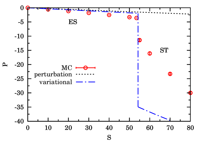
Figure 1: Shows the behavior of the potential energy $P$ as a function of the coupling constant $S$. The points are the MC results (see Tab. 1), the dashed line is the second order perturbation theory result (perturbation) and the dot-dashed line is the variational approach from Ref. A. Sumi and Y. Toyozawa (1973) (variational) in the weak and strong coupling regimes.

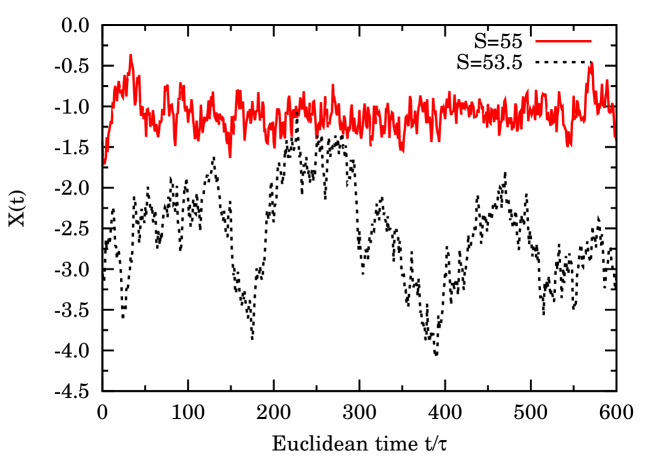
Figure 2: The polaron closed path ${\mbox{\boldmath$x$}}(t)=(X(t),Y(t),Z(t))$ as a function of Euclidean time $t$ in units of $\tau$.

Note that since $S$ and $\tau$ appear in the combination $S\tau^{2}$ in ${\cal U}$ (and $S\tau$ in ${\cal P}$) the same phase transition from an ES to a ST state will be observed increasing the temperature. With the same Hamiltonian we are able to describe two very different behaviors of the acoustic polaron as the temperature changes.

VI Conclusions

In conclusion we used for the first time a specialized PIMC method to study the low temperature behavior of an acoustic polaron. At an inverse temperature $\beta=15$, close to the ground state of the polaron, and at a non-adiabatic parameter $\gamma=0.02$, typical of ionic crystals, we found numerical evidence for a phase transition between an ES state in the weak coupling regime and a ST one in the strong coupling regime at a value of the phonons-electron coupling constant $S^{\star}=54.3(7)$ in good agreement with the prediction of Ref. A. Sumi and Y. Toyozawa (1973), $S^{\star}\sim 1/\gamma$, and the MC simulations of Ref. X. Wang (1998).

To understand the motion of an electron in a deformable lattice we have to consider the fact that the interaction of the electron with the acoustic phonons induces a well barrier proportional to the coupling constant, but it decays due to the retarded property. In the weak coupling region, the electron can easily tunnel through the barrier so that it almost freely moves in the lattice. One can regard the tunneling of the electron as an indication of the motion of the polaron. In this case, a few phonons are involved and the acoustic polaron has a small mass which has a similar magnitude to the mass of the electron and a large radius. In the strong coupling region, the well barrier becomes sufficiently deep and the electron is temporarily bounded in the polaron and cannot tunnel through the barrier until it gains enough energy from the phonons. Much more phonons are involved in the polaron and the mass of the polaron becomes much greater than that of the electron with a small radius. In this argument the specific form of the interaction vertex is of fundamental importance.

We used for the first time a PIMC with the bisection method and correlated sampling as an unbiased numerical mean to probe the low temperature properties of the acoustic polaron. This is an independent route to the Feynman’s variational approach and proved to give reliable results on the existence of the ST state for the electron in a deformable lattice as conceived by Landau. However, the self-trapping we observe in our numerical analysis is not a complete localization of the electron within the polarization cloud of the phonons. The electron path still undergoes small, nearly uncorrelated, fluctuations in Euclidean time in this ST state. Our numerical results support the presence of a discontinuity in the potential energy as a function of the coupling constant and this would be an indication of the existence of a phase transition between the ES and the ST states even if we found no trace of a translational symmetry breaking. Moreover The discontinuity of the ES/ST transition, if it exists, may depend on the cutoff parameter as pointed out by e.g. Ref. F. M. Peeters and J. T. Devreese (1982). In the cold atoms context the role of this parameter is important and the existence of a discontinuous transition is more questionable than in the solid state polaron case J. Tempere, W. Casteels, M. K. Oberthaler, S. Knoop, E. Timmermans, and J. T. Devreese (2009). The present study reports a single value study of the acoustic polaron case thus restricting the generality of the conclusions.

In a truly localized state the polaron should not diffuse at all (strong localization) or at least should attain a subdiffusive behavior (weak localization). But these properties can be checked by looking at the real time dynamics of the system and cannot be checked by the Monte Carlo methods as that used in this work which deals with polaron properties in imaginary time. Clearly our numerical MC results support the claim of a dicontinuity but do not give any proof of a localization transition.

A possible further study could involve the dynamic properties associated with the two different types of motion and bipolarons for short range interacting systems.