Stability of the replica symmetric solution in diluted perceptron learning

Abstract

We study the role played by the dilution in the average behavior of a perceptron model with continuous coupling with the replica method. We analyze the stability of the replica symmetric solution as a function of the dilution field for the generalization and memorization problems. Thanks to a Gardner like stability analysis we show that at any fixed ratio $\alpha$ between the number of patterns $M$ and the dimension $N$ of the perceptron ($\alpha=M/N$), there exists a critical dilution field $h_{c}$ above which the replica symmetric ansatz becomes unstable.

Introduction

Neural networks [1] have become among the most studied and successful models in the field of artificial intelligence. In spite of more than 50 years of research, the field is still thriving [2, 3, 4]. In the last years, thanks to the advances of the new-generation high-throughput technologies in molecular biology, the field has experienced a renewed interest with problems coming from the analysis of high dimensional data in biology, where sparsity in the underlying model is a general feature [5, 6, 7, 8, 3, 4].

In this paper we address the issue of the stability of the replica symmetric solution presented in [9] which has important implications for the implementation of many algorithmic strategies. This paper extends thus the analysis presented in [9] and generalizes the stability results of [10] to the external dilution case.

A standard problem in artificial intelligence is that of generalization [11, 10]. A set of $M$ patterns $\vec{x}^{\mu}$ is given together with a binary output variable $y^{\mu}$ for each of them ($\mu\in\{1,2,\dots,M\}$). A pattern $\vec{x}$ is an $N$ dimensional vector and we are interested in learning the hidden relation among its components and the classification value $y^{\mu}$ related to pattern $\mu$. In the simplest setup, a linear perceptron tries to encode such relation in a vector $\vec{J}$ (called student) such that the binary classification $y^{\mu}=\pm 1$ is reproduced by

$$y^{\mu}=\mathrm{Sign}(\vec{J}\cdot\vec{x}^{\mu})$$

We will consider that the classification is actually generated by an unknown teacher $\vec{J^{0}}$

$$y^{\mu}=\mathrm{Sign}(\vec{J^{0}}\cdot\vec{x}^{\mu}+\eta^{\mu})$$ (1)

and therefore, the aim of the student $\vec{J}$ is to be as close as possible to the teacher $\vec{J^{0}}$. A Gaussian noise $\eta^{\mu}\sim N(0,\gamma^{2})$ is added to the classification function to account for experimental noise in the data. Two interesting limits are studied: no noise $\gamma=0$, and random classification $\gamma=\infty$.

As a first step to analyze the problem, we define an energy function counting the number of patterns that are wrongly classified by the student $\vec{J}$:

$$E(\vec{J})=\sum_{\mu}^{M}\Theta(-y^{\mu}\vec{J}\cdot\vec{x}^{\mu}).$$ (2)

In the following we will consider only the case $J\in{\cal R}^{N}$. Since the energy expression depend only on the angle of $\vec{J}$ and not on his length, i.e. $E(c\vec{J})=E(\vec{J})$ for all $c>0$, we restrict ourself to the surface of a sphere $\sum_{i=1}^{N}J_{i}^{2}=N$.

Standard statistical mechanics method [12, 13, 14, 3, 6] have been largely used to study the thermodynamic properties of this problem. In a recent work [9] a slightly different point of view has been analyzed: which is the $\vec{J}$ that minimizes the energy function with the largest possible number of coordinates equal to zero or, in other words, which is the sparsest possible $\vec{J}$ compatible with a correct classification? To address this issue one needs to study the performance of perceptron in presence of an external dilution field $h$ coupled to the classification vector $\vec{J}$. To this end one can consider the following Hamiltonian:

$$\beta\mathcal{H}(\vec{J})=\beta E(\vec{J})+h\|\vec{J}\|_{p}$$ (3)

where the dilution field $h$, in the last term, acts as a chemical potential on $\vec{J}$. Two interesting cases were studied at the replica symmetric level: the $L_{1}$ norm ($\|\vec{J}\|_{1}=\sum_{i=1}^{N}|J_{i}|$) and the $L_{0}$ norm ($\|\vec{J}\|_{0}=\lim_{p\to 0}\sum_{i=1}^{N}|J_{i}|^{p}=\sum_{i=1}^{N}(1-\delta_{J_{i}})$).

Of course this problem has practical interest in the case one knows a priori when the teacher is actually sparse. In many real life problems [3, 4, 5, 7] the multidimensional patterns $\vec{x}$ contain irrelevant information, in the sense that only few of the components are actually considered in the classification process. We will consider that only a fraction $n_{\mbox{\tiny eff}}^{0}$ of the teacher’s components are non zero. Therefore each teacher’s component is extracted independently from the distribution

$$\rho(J_{0})=(1-n_{\mbox{\tiny eff}}^{0})\delta_{J_{0}}+n_{\mbox{\tiny eff}}^{0}\rho^{\prime}(J_{0}).$$ (4)

It has been shown [8, 5] that dilution with $L_{p}$ norm, with $p\leq 1$, forces a fraction of the components of $\vec{J}$ to be exactly zero, and therefore, allows a selection of the components that actively participate in the classification process.

The cost function $\mathcal{H}(\vec{J})$ raises severe computational problems due to the scale invariance of the energy which makes the optimization problem non-convex in general. At odd with problems like compressed sensing [15], for which optimization methods of order $O(N^{3})$ can be used for the $L_{1}$ norm [5] whereas the most effective $L_{0}$ norm [5] makes the minimization an NP-hard optimization problem [3, 5], in our perceptron-like case we are not aware of any ad-hoc numerical technique for finding efficiently the minimum of the cost function in Eq. (3), apart from Monte Carlo based optimization methods.

From a theoretical perspective, we are interested in the average case properties of the structure of the solution space in either cases $L_{1}$ and $L_{0}$. The paper is organized in the following way: the next section (I) fixes the notation and sketches the replica symmetric results presented in [9], in section II we study the stability of this replica symmetric solution, in section III we show that at $h=0$ the replica symmetric solution is always stable, while at $h\to\infty$ is always unstable, and therefore a critical value of the dilution field marks the threshold between two phases, computed in section IV. Finally, our results are summarized in section V, and the main results of [9] are re-evaluated in the present context.

I Replica symmetric solution to diluted perceptron

Using the replica method [16, 12] one can compute the average free energy as the limit $-\beta\overline{f}=\lim_{n\to 0}$ $\lim_{N\to\infty}\log\overline{Z^{n}}/nN$. The replica symmetric (RS) ansatz assumes that any two replicas of the system have the same overlap, and therefore the corresponding overlap matrix and its Fourier conjugate assume the following structure:

$$Q_{a,b}=\left(\begin{array}[]{ccccc}t&&&&\\ r&1&&&\\ r&q&1&&\\ .&.&.&1&\\ r&q&.&q&1\end{array}\right)\quad-i\hat{Q}_{a,b}=\left(\begin{array}[]{ccccc}\lambda^{0}&&&&\\ \hat{r}&\lambda&&&\\ \hat{r}&\hat{q}&\lambda&&\\ .&.&.&\lambda&\\ \hat{r}&\hat{q}&.&\hat{q}&\lambda\end{array}\right)$$ (5)

These are symmetric $(n+1)\times(n+1)$ matrices where the first column (row) contains the teacher’s parameters. For instance, $t$ is the variance of the teacher and is related to the distribution (4), and is not a variational parameter. On the other hand, $r=\langle\frac{1}{N}\vec{J}\cdot\vec{J^{0}}\rangle$ is the average overlap between the teacher and the student, and $q=\langle\frac{1}{N}\vec{J}^{a}\cdot\vec{J}^{b}\rangle$ is the average overlap between two replicas (see [9] for details).

The correct value for the free energy is obtained by minimizing the variational RS free energy

$$-\beta\overline{f}=-r\hat{r}+\frac{1}{2}q\hat{q}-\lambda+G_{J}+\alpha\>G_{X}$$

with respect to the variational parameters $(q,r,\hat{q},\hat{r},\lambda)$, where

$$G_{J} = \int\mathrm{D}x\>\int\mathrm{d}J^{0}\rho(J^{0})\log\int\mathrm{d}Je^{-(\frac{\hat{q}}{2}-\lambda)J^{2}-h\|J\|_{p}+(\hat{r}J^{0}-\sqrt{\hat{q}}x)J}$$ (6)

$$G_{X} = 2\int\mathrm{D}x\>H\left(\frac{xr}{\sqrt{q\gamma^{2}+qt-r^{2})}}\right)\log\left((e^{-\beta}-1)H(-\sqrt{\frac{q}{1-q}}x)+1\right)$$

In these equations, and from now on, $\mathrm{D}x\>=\mathrm{d}x\>\exp(-x^{2}/2)/\sqrt{2\pi}$ is a Gaussian measure in $x$, and the function $H(y)=\displaystyle\int_{y}^{\infty}\mathrm{D}x\>$.

A key role is played by $\alpha=\frac{M}{N}$, the ratio between the number of patterns $M$ and the space dimensionality $N$, that measures the amount of information we have and, together with $h$, is the fundamental parameter controlling the quality of the generalization. We assume that in the limit $N\rightarrow\infty$, $\alpha$ remains finite.

II Stability a la Gardner

The main goal of this work is to analyze the stability of the replica symmetric solution. Other structures for the overlap matrices (5) are indeed possible. In analogy with the organization of the thermodynamic states in the low temperature phase of mean field spin glass-like models [16], we expect that the space of solutions of our model could be described by a hierarchical (ultrametric) organization of replicas, or, in other terms, that our system might undergo a spontaneous replica symmetry breaking (RSB). From a purely geometric point of view this process is related to the fragmentation of the space of zero energy configurations into unconnected regions, or equivalently, the fragmentation of the Gibbs measure into many pure states:

Figure 1: Representation of a connected (left) and a disconnected (right) solution space on the sphere. Connected phase space is typical of replica symmetric solutions, while the breaking in the symmetry of the replicas implies the clusterization of the space.

We will now apply Gardner’s method for the stability analysis of replica symmetric solution in [13], studying the eigenvalues of the Hessian matrix:

$$\|\partial^{2}(\beta n\overline{f_{n}})\|=\left(\begin{array}[]{ccccccc}\|\frac{\partial^{2}(\beta n\overline{f_{n}})}{\partial Q_{ab}\partial Q_{cd}}\|&&&\|\frac{\partial^{2}(\beta n\overline{f_{n}})}{\partial Q_{ab}\partial(-\imath\hat{Q}_{cd})}\|\\ \|\frac{\partial^{2}(\beta n\overline{f_{n}})}{\partial Q_{ab}\partial(-\imath\hat{Q}_{cd})}\|&&&\|\frac{\partial^{2}(\beta n\overline{f_{n}})}{\partial(-\imath\hat{Q}_{ab})\partial(-\imath\hat{Q}_{cd})}\|\end{array}\right)$$ (7)

evaluated at the RS fixed point. Details of the calculation are given in the Appendix A.

The eigenvalues of the $n(n+1)\times n(n+1)$ Hessian matrix are simply related to the spectrum of the four sub-matrices. Among the eigenvectors only those with eigenvalues $\delta_{1}$ and $\delta_{2}$, signal an instability of the replica symmetric solution:

$$\delta_{1}\delta_{2}=\gamma_{1}\gamma_{2}-1$$ (8)

where $\gamma_{1}$ and $\gamma_{2}$ are eigenvalues of the inner matrices $\|\frac{\partial^{2}(\beta n\overline{f_{n}})}{\partial Q_{ab}\partial Q_{cd}}\|$ and $\|\frac{\partial^{2}(\beta n\overline{f_{n}})}{\partial(-\imath\hat{Q}_{ab})\partial(-\imath\hat{Q}_{cd})}\|$, given by

$$\gamma_{1} = -\frac{2\alpha}{(1-q)^{2}}\int\mathrm{D}y\>H\left(\frac{yr}{\sqrt{q\gamma^{2}+qt-r^{2}}}\right)\left\{\left(\frac{e^{-\frac{h_{0}^{2}}{2}}}{\sqrt{2\pi}(H(h_{0})-1)}\right)^{2}-\frac{h_{0}e^{-\frac{h_{0}^{2}}{2}}}{\sqrt{2\pi}(H(h_{0})-1)}\right\}^{2}$$

$$\gamma_{2} = -\int\mathrm{D}z\>\int\mathrm{d}J^{0}\rho(J^{0})\left\{\frac{\int\mathrm{d}JJ^{2}e^{H_{J}}}{\int\mathrm{d}Je^{H_{J}}}-\left(\frac{\int\mathrm{d}JJe^{H_{J}}}{\int\mathrm{d}Je^{H_{J}}}\right)^{2}\right\}^{2}.$$ (9)

where $H_{J}=-(\frac{\hat{q}}{2}-\lambda)J^{2}+(\hat{r}J_{0}-\sqrt{\hat{q}}x)J-h|J|^{p}$.

The sign of the product $\delta_{1}\delta_{2}$ determines the stability of the extremal point: when $\delta_{1}\delta_{2}<0$ the point is stable, and unstable otherwise.

III Extreme cases: $h=0$ and $h\to\infty$

In the zero temperature case, the Gibbs measure concentrates over the states of lower energy, i.e. over those vectors $\vec{J}$ that correctly classify most patterns. In the absence of dilution ($h=0$), the measure is uniform over these states, and the free energy is thus a measure of their entropy (we are working at zero temperature). On the other extreme, we have the high dilution limit $h\to\infty$ that we studied in [9] at replica symmetric level. Next we check the stability of the replica symmetric solution for both the Memorization and Generalization problems in these two extreme situations. As we will see, the replica symmetric solution is stable for $h=0$ and unstable for $h\to\infty$, and therefore, there is a critical value $h_{c}(\alpha)$ dividing the RS phase from the non-RS one.

III.1 Stability of non diluted perceptron $h=0$

In the absence of dilution ($h=0$) we still have two cases: memorization ($\gamma\to\infty$) and generalization ($\gamma=0$). In the high noise limit $\gamma\rightarrow\infty$ (see eq. (1)) there is no rule to infer because the experiments are randomly classified, and the perceptron tries to memorizes the output variable $y^{\mu}$. In the $\gamma=0$ case, the patterns are classified according to the teacher and this rule can be generalized.

In the memorization limit ($\gamma\to\infty$), an RS solution of zero energy always exists for $0<\alpha<2$ [13]. For these values of $\alpha$ the student is capable of memorizing the experiments, whereas for $\alpha>2$ there are no zero energy solutions, and, solutions are not replica symmetric. In agreement with this known behavior (see [13]), the product of the eigenvalues $\delta_{1}\delta_{2}$, evaluated in the non diluted memorization replica symmetric solution, is negative for $\alpha<2$. Its value grows from $-1$ at $\alpha=0$ to $0$ at $\alpha=2$ (Figure 2), an indication that the zero energy replica symmetric solution is stable in this range.

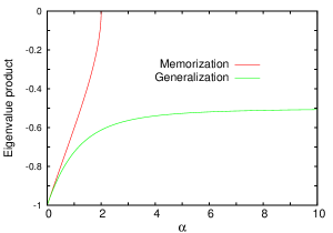
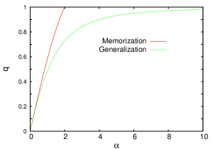
Figure 2: The eigenvalues product (left) evaluated in the replica symmetric solution for the generalization and memorization non diluted. The corresponding self-overlap $q$ of the student (right).

In the generalization limit ($\gamma=0$) the perceptron can asymptotically learn the classification rule provided with a big enough amount of data as shown in [9]. However, for any finite amount of information $\alpha$, there is not just one zero-cost student, but a continuum of them filling a bounded region of the $J$’s space (see left panel of Fig. 1). An indication of the size of the solution space is given by the student-student overlap $q=\langle J^{a}J^{b}\rangle$. As in the memorization case (for $\alpha<2$), the solution space is connected, and, consistently in this case the product $\delta_{1}\delta_{2}$ remains always negative (see Fig. 2), which means that the replica symmetric solution is stable for every $\alpha$ as in [10]. As $\alpha\to\infty$ the solutions space shrinks around the correct value $\vec{J^{0}}$, and $q\to 1$ (see Fig. 2).

As expected, as little information is given to the student (low values of $\alpha$), there is little difference between the memorization and the generalization. Figure 2 shows that also the stability, given by the product $\delta_{1}\delta_{2}$ for the non diluted generalization and memorization coincides for small $\alpha$ and have the same limit for $\alpha\rightarrow 0^{+}$.

III.2 Stability of diluted perceptron $h=\infty$

The dilution field select those solutions with the lowest values of the norm. In particular, $L_{0}$ and $L_{1}$ norms are known to force the sparsity of the solutions [8], pushing a fraction of the students components to be zero. Seeking for sparse solutions can enhance the efficiency in the use of available information [8, 7, 5, 6], in particular when the teacher is actually sparse. In the following we will consider a $95\%$ sparse teacher, i.e. $n_{\mbox{\tiny eff}}^{0}=0.05$ in Eq. (4).

The behavior of large dilution field $h\rightarrow\infty$ limit depends on the norm used and so does the learning behavior of the perceptron [9]. We restrict ourselves to the study of the space of $E=0$ solutions: to do so we take the limit $T\to 0$ first, and then the limit $h\to\infty$. Again in [9] it was shown that, in the replica symmetric case, $h\to\infty$ pushes $q\to 1$ at any $\alpha$, concentrating the Gibbs measure over a single point: the most diluted zero energy $\vec{J}$. However, the question remains as whether the replica symmetric ansatz is still valid or the strong dilution field fractures the Gibbs measures into unconnected components.

In figure 3 we show the eigenvalues product for the $L_{0}$ and $L_{1}$ dilutions in the $h\to\infty$ limit for both, the memorization and the generalization cases. At variance with the non diluted case, the $h=\infty$ one is always unstable.

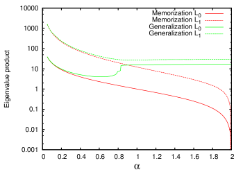
Figure 3: The eigenvalues product evaluated in the replica symmetric solution for the $L_{0}$ and the $L_{1}$ norms in generalization and memorization.

IV Phase diagram

In the region of $\alpha$ where perfect memorization/generalization is possible, the replica symmetric ansatz is stable in absence of dilution and unstable in presence of a very strong dilution field $h\to\infty$. Therefore there should exist a critical value for the dilution field $h_{c}(\alpha)$ separating the RS from the RSB phase. In figure 4 we show $h_{c}(\alpha)$ for the $L_{1}$ and the $p=0.1$ norms applied to models with different teachers dilutions.

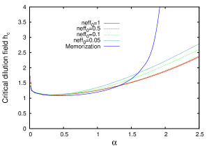
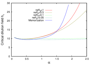
Figure 4: The phase diagram for the $L_{1}$(left) and the $p=0.1$(right) norms with severals teacher’s dilution $n_{eff}^{0}$. The replica symmetric solution is stable for values of $\alpha$ and $h$ below the lines.

The similarity of the stability curves near $\alpha=0$ is because with such a few information there is not big difference between memorizing and generalizing. The curves separate around $\alpha\gtrsim 0.4$. The value of the critical dilution field increases with $\alpha$. This can be rationalized as follows: more information implies a reduction in the size of the $E=0$ solution space, and therefore different solutions are closer, so a higher dilution field is needed to clusterize the set of zero energy students. In generalization, when $\alpha\rightarrow\infty$ the solution space is composed by an only vector which is precisely the teacher and the replica-replica overlap $q$ achieves its maximum value $1$, consequently the critical curves go to infinity too. For the memorization case, the value $q=1$ is achieved for $\alpha=2$, that’s why the critical curve diverges here.

Drawing the critical lines for the $L_{0}$ norm is not obvious because setting $p=0$ in the equations, before taking the strong dilution limit $h\rightarrow\infty$, eliminates the effect of any finite dilution field, so there is no way to find $h_{c}$ (see [9]). What we have done instead is to study the critical lines for a value of the norm exponent $p$ small enough. The results using $p=0.1$ are shown in the right panel of Fig. 4. Again, around $\alpha=0$ both, memorization and generalization, behave similarly. The memorization critical line also diverges when $\alpha\rightarrow 2$ while the generalization ones increases with $\alpha$ as for the $L_{1}$ norm. In both cases, $L_{1}$ and $L_{0.1}$, the critical field $h_{c}(\alpha)$ depends on the sparsity $n_{\mbox{\tiny eff}}^{0}$ of the teacher (eq. (4)).

V Conclusions

We have performed a full stability analysis of the replica symmetric solution for the non diluted and diluted generalization and memorization problems for a learning perceptron. Imposing a dilution should improve the results obtained in real algorithms, but comes with a price. We showed that even in the satisfiable phase (where zero cost solutions exists) an infinite dilution breaks the symmetry of the replicas, whereas no dilution at all keep the replica symmetric solution stable. The breaking of the symmetry is usually connected with convergence problems in algorithms like belief propagation. Yet, it is always possible to find a dilution field weak enough for the replica symmetric solution to be stable, provided it exists. The critical dilution field $h_{c}(\alpha)$ depends on the actual sparseness of the teacher.

Figure 5, partially taken from [9], shows the generalization error achieved in average case by a perceptron without a dilution filed, and with a very strong ($h\to\infty$) dilution field. The teacher used is quite sparse ($n_{\mbox{\tiny eff}}^{0}=5\%$), and therefore the learning process is enhanced by the use of dilution. Restricting ourselves to the replica symmetric space, the $h\to\infty$ limit is not achievable, and $h_{c}(\alpha)$ is the best we can do. The gain in accuracy (lower error) obtained with an $h_{c}$-diluted perceptron is not as impressive as the $h\to\infty$ case, but still improves the results without dilution.

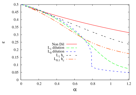
Figure 5: First three lines (in caption order) are the generalization error obtained without dilution and with strong $h\to\infty$ dilution for the $L_{1}$ and $L_{0}$ norms (results taken from [9]). The last two lines correspond to the generalization error obtained with $h=h_{c}(\alpha)$ in the $L_{1}$ and $L_{0.1}$ cases.

The present work is useful as it defines the phase space of the replica symmetric solution in the information-dilution ($\alpha-h$) plane. The actual relation of this predictions to the behavior of algorithms remains as an open project for the future. Also left for the future is the use of 1RSB (or higher) parameters to make average predictions in the RSB phase.

Appendix A Details of the stability calculation

The variational free energy in terms of the all $Q_{a,b}$ and their Fourier counterparts is (see [9]), after taking the $N\rightarrow\infty$, given by

$$\beta n\overline{f_{n}} = -\imath\sum_{a\leq b}Q_{ab}\hat{Q}_{ab}-$$

$$-\log\int\prod_{a=0}^{n}\mathrm{d}J^{a}\int\mathrm{d}J^{0}\rho(J^{0})e^{-h\sum_{a}\|J^{a}\|_{p}^{p}-\imath\sum_{a\leq b}\hat{Q}_{ab}J^{a}J^{b}}-$$

$$-\alpha\log\int\mathrm{D}\eta\>\prod_{a=0}^{n}\frac{\mathrm{d}x^{a}\mathrm{d}\hat{x^{a}}}{\sqrt{2\pi}}e^{-\beta\sum_{a=1}^{n}\theta(-x^{a}(x^{0}+\eta))+\imath\sum_{a=1}^{n}x^{a}\hat{x^{a}}-\frac{1}{2}\sum_{a,b}^{n}Q_{ab}\hat{x^{a}}\hat{x^{b}}}$$

Deriving respect to its $(n+1)(n+2)$ parameters $Q_{ab}$ and $\hat{Q}_{ab}$, one can construct the second derivatives matrix or Hessian of $\beta n\overline{f_{n}}$ .The sign of the eigenvalues of this matrix evaluated in an extremal point will give us all the information about its stability.

The free energy second derivatives are

$$\frac{\partial^{2}(\beta n\overline{f_{n}})}{\partial Q_{ab}\partial Q_{cd}} = \alpha(1-\frac{\delta_{ab}}{2})(1-\frac{\delta_{cd}}{2})(\langle\hat{x^{a}}\hat{x^{b}}\rangle\langle\hat{x^{c}}\hat{x^{d}}\rangle-\langle\hat{x^{a}}\hat{x^{b}}\hat{x^{c}}\hat{x^{d}}\rangle)$$

$$\frac{\partial^{2}(\beta n\overline{f_{n}})}{\partial(-\imath\hat{Q}_{ab})\partial(-\imath\hat{Q}_{cd})} = \langle J^{a}J^{b}J^{c}J^{d}\rangle-\langle J^{a}J^{b}\rangle\langle J^{c}J^{d}\rangle$$

$$\frac{\partial^{2}(\beta n\overline{f_{n}})}{\partial Q_{ab}\partial(-\imath\hat{Q}_{cd})} = \delta_{ab,cd}$$

where

$$\langle g(\hat{x^{a}},\hat{x^{b}},...)\rangle = \frac{\int\mathrm{D}\eta\>\prod_{a=0}^{n}\frac{\mathrm{d}x^{a}\mathrm{d}\hat{x^{a}}}{\sqrt{2pi}}g(\hat{x^{a}},\hat{x^{b}},...)e^{-\beta\sum_{a=1}^{n}\theta(-x^{a}(x^{0}+\eta))+\imath\sum_{a=1}^{n}x^{a}\hat{x^{a}}-\frac{1}{2}\sum_{a,b}^{n}Q_{ab}\hat{x^{a}}\hat{x^{b}}}}{\int\mathrm{D}\eta\>\prod_{a=0}^{n}\frac{\mathrm{d}x^{a}\mathrm{d}\hat{x^{a}}}{\sqrt{2pi}}e^{-\beta\sum_{a=1}^{n}\theta(-x^{a}(x^{0}+\eta))+\imath\sum_{a=1}^{n}x^{a}\hat{x^{a}}-\frac{1}{2}\sum_{a,b}^{n}Q_{ab}\hat{x^{a}}\hat{x^{b}}}}$$

$$\langle g(J^{a},J^{b},...)\rangle = \frac{\int\prod_{a=0}^{n}\mathrm{d}J^{a}\int\mathrm{d}J^{0}\rho(J^{0})g(J^{a},J^{b},...)e^{-h\sum_{a}\|J^{a}\|_{p}^{p}-\imath\sum_{a\leq b}\hat{Q}_{ab}J^{a}J^{b}}}{\int\prod_{a=0}^{n}\mathrm{d}J^{a}\int\mathrm{d}J^{0}\rho(J^{0})e^{-h\sum_{a}\|J^{a}\|_{p}^{p}-\imath\sum_{a\leq b}\hat{Q}_{ab}J^{a}J^{b}}}$$

The structure of the Hessian matrix is:

$$\|\partial^{2}(\beta n\overline{f_{n}})\|=\left(\begin{array}[]{ccccccc}\|\frac{\partial^{2}(\beta n\overline{f_{n}})}{\partial Q_{ab}\partial Q_{cd}}\|&&&\|\frac{\partial^{2}(\beta n\overline{f_{n}})}{\partial Q_{ab}\partial(-\imath\hat{Q}_{cd})}\|\\ \|\frac{\partial^{2}(\beta n\overline{f_{n}})}{\partial Q_{ab}\partial(-\imath\hat{Q}_{cd})}\|&&&\|\frac{\partial^{2}(\beta n\overline{f_{n}})}{\partial(-\imath\hat{Q}_{ab})\partial(-\imath\hat{Q}_{cd})}\|\end{array}\right)$$ (10)

The eigenvector space of the Hessian matrix can be divided in two [13, 12, 17]; one subspace corresponding to instabilities inside the replica symmetric space (and whose eigenvalues signs are those who determines among of all the possible replica symmetric solutions the one who actually minimizes the free energy), and the other corresponding to instabilities that takes our extremal point outside the replica symmetric space. The first of these subspaces has no interest to our stability analysis, because solving the replica symmetric fixed point equations is equivalent to searching for the stable extremal replica symmetric point, so, we are going to focus on the eigenvalues of the eigenvectors belonging to the second subspace. A detailed study of the Hessian matrix shows that it has just two non replica symmetric values, $\delta_{1}$ and $\delta_{2}$. The product $\delta_{1}\delta_{2}$ can be expressed as in eq. (8) in terms of the eigenvalues of the inner matrices.

References

- [1] Trevor Hastie, Robert Tibshirani, and Jerome Friedman. The Elements of Statistical Learning. Springer, 2009.
- [2] Alfredo Braunstein and Riccardo Zecchina. Learning by message passing in networks of discrete synapses. Phys. Rev. Lett., 96:030201, Jan 2006.
- [3] A Braunstein, A Pagani, M Weigt, and R Zecchina. Inference algorithms for gene networks: A statistical-mechanics analysis. Journal of Statistical Mechanics: Theory and Experiment, 2008(12), 2008.
- [4] Andrea Pagnani, Francesca Tria, and Martin Weigt. Classification and sparse-signature extraction from gene-expression data. Journal of Statistical Mechanics: Theory and Experiment, 2009(05):P05001, 2009.
- [5] Y Kabashima, T Wadayama, and T Tanaka. A typical reconstruction limit for compressed sensing based on l p -norm minimization. Journal of Statistical Mechanics: Theory and Experiment, 2009(09):L09003, 2009.
- [6] T Wadayama Y Kabashima and T Tanaka. Statistical mechanics analysis of a typical reconstruccion limit of compressed sensing. Information theory proceedings, 2010 IEEE, pages 1533 – 1537, 2010.
- [7] F. Krzakala, M. Mézard, F. Sausset, Y. F. Sun, and L. Zdeborová. Statistical-physics-based reconstruction in compressed sensing. Phys. Rev. X, 2:021005, May 2012.
- [8] Robert Tibshirani. Regression shrinkage and selection via the lasso. Journal of the Royal Statistical Society, Series B, 58:267–288, 1994.
- [9] A Lage-Castellanos, A Pagnani, and M Weigt. Statistical mechanichs of sparse generalization and model selection. J. Stat. Mech.: Theor. Exp., page P12001, 2009.
- [10] T Geszti I Derényi and G Györgyi. Generalization in the programed teaching of a perceptron. Physical Review E, 50(4):3192–3200, 1994.
- [11] F Vallet. The hebb rule for learning separable boolen functions: learning and generalization. Europhys. Lett., 8:747–751, 1989.
- [12] A. Engel and C. Van der Broeck. Statistical Mechanics of Learning. Cambidge University Press, 2001.
- [13] E Gardner and B Derrida. Optimal storage properties of neural network models. Journal of Physics A: Mathematical and General, 21(1):271–284, 1988.
- [14] E Gardner. The space of interactions in neural network models. Journal of Physics A: Mathematical and General, 21(1):257–270, 1988.
- [15] D.L. Donoho. Comressed sensing. IEEE Trans. on Information Theory, 52:1289–1306, 2006.
- [16] M. Mézard, G. Parisi, and M.A. Virasoro. Spin Glass Theory and Beyond. World Scientific, Singapore, 1987.
- [17] J R L de Almeida and D J Thouless. Stability of the sherrington-kirkpatrick solution of a spin glass model. J. Phys. A: Math. Gen., 11(5), 1978.