Efficient quantum algorithm to construct arbitrary Dicke states

Abstract

In this paper, we study efficient algorithms towards the construction of any arbitrary Dicke state. Our contribution is to use proper symmetric Boolean functions that involve manipulations with Krawtchouk polynomials. Deutsch-Jozsa algorithm, Grover algorithm and the parity measurement technique are stitched together to devise the complete algorithm. Further, motivated by the work of Childs et al (2002), we explore how one can plug the biased Hadamard transformation in our strategy. Our work compares fairly with the results of Childs et al (2002).

Keywords: Biased Hadamard Transform, Deutsch-Jozsa Algorithm, Dicke State, Grover Algorithm, Krawtchouk Polynomial, Parity Measurement, Symmetric Boolean Functions.

I Introduction

Multipartite entanglement is one of the important areas in the field of quantum information that has many applications including quantum secret sharing. In this paper, we focus on the Dicke states PhysRev.93.99 , which are useful building blocks in realizing multipartite entanglement. The $n$-qubit weight $w$ Dicke state, $|D^{n}_{w}\rangle$, is the equal superposition of all $n$-qubit states of weight $w$. We refer to dickold ; d2 ; d3 ; phyb ; d1 ; d4 ; d5 and the references therein for detailed discussion.

After the invention of quantum information, many experimental setups have been proposed and tested to verify some theoretical properties. Most of experiments have been focused on the test of multipartite entanglement such as EPR, GHZ, and W states. Since the result of experimental tests depends on the steps for preparing, processing, and measuring, all steps should be refined as much as possible. Among them, the first priority is to prepare the target state with very high fidelity and with efficiency. In this work, therefore, we also focus on the efficient way to prepare certain multipartite quantum state.

In line of GHZ and W states, we have the Dicke state, $|D^{n}_{w}\rangle$, which an equal superposition state of all $n$-qubit states of weight $w$. Actually, Dicke state is more general state than GHZ and W states since W state is $|D^{n}_{1}\rangle$ and GHZ state is the superposition of $|D^{n}_{0}\rangle$ and $|D^{n}_{n}\rangle$. Therefore, the preparation method for Dicke state can be utilized for other general case as well. At the same time, similar to the above reason, Dicke state can be utilized for many applications such as secret sharing d5 and quantum networking dd1 . Related to this, some previous works have been done that focussed on the experimental ways to prepare six-qubit Dicke state d5 ; d4 with fidelity $0.654\pm 0.024$ and $0.56\pm 0.02$, respectively.

While the main focus from the viewpoint of experimental physics is to actually provide the implementation of specific Dicke states, our focus is from theoretical algorithmic angle and the only result presented in this direction appeared in dickold . In this work, we show how one can efficiently construct Dicke states by using the combinatorial properties of symmetric Boolean functions, two well-known quantum algorithms, and the generalized parity measurement. By efficient, we mean that the resource requirements in terms of quantum circuits and number of execution steps is poly$(n)$ to obtain $|D^{n}_{w}\rangle$.

Let us consider $n$-qubit states in the computational basis $\{0,1\}^{n}$ that can be written in the form $\sum_{x\in\{0,1\}^{n}}a_{x}|x\rangle$, where $\sum_{x\in\{0,1\}^{n}}|a_{x}|^{2}=1$. Thus, $x$ can also be interpreted as a binary string and the number of $1$’s in the string is called the (Hamming) weight of $x$ and denoted as $wt(x)$. Based on this an arbitrary Dicke state can be expressed as follows:

$$|D^{n}_{w}\rangle=\sum\limits_{x\in\{0,1\}^{n},wt(x)=w}\frac{1}{\sqrt{\binom{n}{w}}}|x\rangle.$$

Let us also define a symmetric $n$-qubit state as

$$|S^{n}\rangle=\sum_{x\in\{0,1\}^{n}}a_{wt(x)}|x\rangle,\mbox{ where }\sum_{i=0}^{n}\binom{n}{i}|a_{i}|^{2}=1.$$

First, we show how one can prepare a symmetric $n$-qubit state with the property that $\binom{n}{w}|a_{w}|^{2}$ is $\Omega(\frac{1}{\sqrt{n}})$ by using Deutsch-Jozsa algorithm qDJ92 . This requires certain novel combinatorial observations related to symmetric Boolean functions. Then the quantum state out of Deutsch-Jozsa algorithm is measured using the parity measurement technique d2 to obtain $|D^{n}_{w}\rangle$ with a probability $\Omega(\frac{1}{\sqrt{n}})$. Thus, $O(\sqrt{n})$ runs are sufficient to obtain the required Dicke state. Note that a direct approach to construct a symmetric state has been presented in dickold using biased Hadamard transform. While the order of probability to obtain Dicke state by ours and that of dickold are the same, enumeration results show that the exact probability values are better in our case than that of dickold .

Further, motivated by the idea in dickold , we improve our algorithm further with a modified Deutsch-Jozsa operator that involves the biased Hadamard transform. Since biased Hadamard transform also helps to generate the target symmetric state, the overall probability to obtain the Dicke state increases.

Finally, we can also apply the Grover operator qGR96 before the measurement. Since Grover algorithm amplifies the amplitude of target symmetric state, this helps to reduce the necessary number of steps into $O(\sqrt[4]{n})$.

II Properties of Symmetric Boolean Functions

II.1 Walsh Spectrum of Symmetric Boolean Functions

A Boolean function on $n$ variables may be viewed as a mapping from $\{0,1\}^{n}$ into $\{0,1\}$. Let us denote the addition operator over $GF(2)$ by $\oplus$. Let ${x}=(x_{1},\ldots,x_{n})$ and ${\omega}=(\omega_{1},\ldots,\omega_{n})$ both belong to $\{0,1\}^{n}$ and the inner product

$${x}\cdot{\omega}=x_{1}\omega_{1}\oplus\cdots\oplus x_{n}\omega_{n}.$$

Let $f({x})$ be a Boolean function on $n$ variables. Then the Walsh transform of $f({x})$ is a real valued function over $\{0,1\}^{n}$ which is defined as

$$W_{f}({\omega})=\sum_{{x}\in\{0,1\}^{n}}(-1)^{f({x})\oplus{x}\cdot{\omega}}.$$

An $n$-variable Boolean function $f$ is called Symmetric if $f(x)=f(y)$ for all $x,y\in\{0,1\}^{n}$ such that $wt(x)=wt(y)$. Henceforth, we will denote the set of $n$-variable symmetric Boolean functions as ${\cal SB}_{n}$.

In the truth table of $f\in{\cal SB}_{n}$, it is enough to provide outputs corresponding to different weights of elements of $\{0,1\}^{n}$ only. So an $n$-variable symmetric function can be expressed by an $(n+1)$ length bit string as

$$re_{f}=[f_{0},f_{1},\ldots,f_{n}],$$

where $f_{i}$ is the output at the inputs of weight $i$ and $re_{f}$ is referred to as the simplified value vector. When $f\in{\cal SB}_{n}$, one may note that $W_{f}(x)=W_{f}(y)$ for all $x,y\in\{0,1\}^{n}$ such that $wt(x)=wt(y)$. Therefore, the Walsh spectrum of $f$ can be represented by an $(n+1)$ length integer string

$$rw_{f}=[rw_{f}(0),rw_{f}(1),\ldots,rw_{f}(n)],$$

where $rw_{f}(i)$ represents the Walsh spectrum value at the inputs of weight $i$.

II.2 Relation between Walsh Spectrum and Krawtchouk polynomials

We now relate the Walsh spectrum of the symmetric functions kws with Krawtchouk polynomials IK96 ; FJ77 . Krawtchouk polynomial of degree $i$ is given by

$$K_{i}(\eta,n)=\sum_{j=0}^{i}(-1)^{j}\binom{\eta}{j}\binom{n-\eta}{i-j}.$$

From kws , we get that if $wt(\omega)=k$, then

$$W_{f}(\omega)=\sum_{i=0}^{n}(-1)^{f_{i}}K_{i}(k,n).$$

The $(n+1)\times(n+1)$ matrix which has $K_{i}(k,n)$ as the $(i,k)$-th element is known as the Krawtchouk matrix krawten ; fein .

For example, let us present the Krawtchouk matrix for $n=5$ and $6$ as follows:

$\left[\begin{array}[]{rrrrrr}1&1&1&1&1&1\\ 5&3&1&-1&-3&-5\\ 10&2&-2&-2&2&10\\ 10&-2&-2&2&2&-10\\ 5&-3&1&1&-3&5\\ 1&-1&1&-1&1&-1\end{array}\right],$ $\left[\begin{array}[]{rrrrrrr}1&1&1&1&1&1&1\\ 6&4&2&0&-2&-4&-6\\ 15&5&-1&-3&-1&5&15\\ 20&0&-4&0&4&0&-20\\ 15&-5&-1&3&-1&-5&15\\ 6&-4&2&0&-2&4&-6\\ 1&-1&1&-1&1&-1&1\end{array}\right].$

In these two matrices, one can verify the properties related to the Krawtchouk matrix given in Proposition 1.

To determine all the Walsh spectrum values of $f\in{\cal SB}_{n}$, it is enough to multiply $((-1)^{f_{0}},\ldots,(-1)^{f_{n}})$ with the $(n+1)\times(n+1)$ Krawtchouk matrix. Applying Krawtchouk matrix, the analysis of the Walsh spectra of symmetric functions becomes combinatorially interesting. Elements of a Krawtchouk matrix have nice combinatorial properties and they follow nice symmetry IK96 too. We list some of them in the following proposition.

Proposition 1

1. $K_{0}(k,n)=1,K_{1}(k,n)=n-2k$,
2. $(i+1)K_{i+1}(k,n)=(n-2k)K_{i}(k,n)$
$-(n-i+1)K_{i-1,n}(k,n)$,
3. $K_{i}(k,n)=(-1)^{k}K_{n-i}(k,n)$,
4. $\binom{n}{k}K_{i}(k,n)=\binom{n}{i}K_{k}(i,n)$,
5. $K_{i}(k,n)=(-1)^{i}K_{i}(n-k,n)$,
6. $(n-k)K_{i}(k+1,n)=(n-2i)K_{i}(k,n)-kK_{i}(k-1,n)$,
7. $(n-i+1)K_{i}(k,n+1)=(3n-2i-2k+1)K_{i}(k,n)$
$-2(n-k)K_{i}(k,n-1)$.

II.3 Implementation of Symmetric Boolean Functions

The symmetric Boolean functions can be efficiently implemented. As described in sympoly , the circuit complexity of $n$-variable symmetric Boolean functions is $4.5n+o(n)$. It is known that given a classical circuit $f$, there is a quantum circuit of comparable efficiency which computes the transformation $U_{f}$ that takes input like $|x,y\rangle$ and produces output like $|x,y\oplus f(x)\rangle$. Thus, we will consider that for $f\in{\cal SB}_{n}$, the quantum circuit $U_{f}$ can be efficiently implemented using $O(n)$ circuit complexity.

III Algorithms

III.1 Find a Special Symmetric Boolean Function which maximizes the Walsh Spectrum

Consider that we want to maximize the Walsh spectrum value corresponding to weight $w$ points and naturally, from the property of symmetric functions, all of them will be equal. Now we present an important combinatorial result to show how to find such symmetric Boolean functions.

Theorem 1

Consider $f\in{\cal SB}_{n}$. The function $f$, represented as $re_{f}$, for which the Walsh spectrum corresponding to the $w$ weight points will be maximized, can be written as

$$f_{i}=\begin{cases}0,&$if$\,\,K_{i}(w,n)>0\\ 1,&$if$\,\,K_{i}(w,n)<0\\ 0\,$or$\,1,&$if$\,\,K_{i}(w,n)=0\end{cases}$$

Proof: We have $W_{f}(\omega)=\sum_{i=0}^{n}(-1)^{f_{i}}K_{i}(k,n)$. One may note that the maximum value of $\sum_{i=0}^{n}(-1)^{f_{i}}K_{i}(k,n)$ is $\sum_{i=0}^{n}|K_{i}(k,n)|$. This is attained when we take the function of the form as described in the theorem.  

Example 1

As example, consider $n=6,w=k=2$. In the corresponding column of the $(6+1)\times(6+1)$ matrix, we get the values as $1,2,-1,-4,-1,2,1$. Thus, we will consider the function with $re_{f}$ as $[0,0,1,1,1,0,0]$. For such an $f\in{\cal SB}_{6}$, the Walsh spectrum values at the points $\omega$, such that $w=wt(\omega)=2$, will be maximized, which is $1+2+1+4+1+2+1=12$.

III.2 Walsh Spectrum of the Special Symmetric Boolean function by Combinatorial Property of Krawtchouk Matrix

Next we present certain results related to column sum of Krawtchouk matrix.

Lemma 1

$\sum_{i=0}^{n}|K_{i}(\lceil\frac{n}{2}\rceil,n)|=\sum_{i=0}^{n}|K_{i}(\lfloor\frac{n}{2}\rfloor,n)|=2^{\lceil\frac{n}{2}\rceil}$.

Proof: Let us first prove this for even $n$.

Following Proposition 1(2), we have

$$(i+1)K_{i+1}(k,n) = (n-2k)K_{i}(k,n)$$

$$-(n-i+1)K_{i-1,n}(k,n).$$

For $n$ even, and $k=\frac{n}{2}$, we get,

$$K_{i+1}(\frac{n}{2},n)=-\frac{n-i+1}{i+1}K_{i-1,n}(\frac{n}{2},n).$$

That is, the recurrence relation follows:

$$K_{i}(\frac{n}{2},n)=-\frac{n-i+2}{i}K_{i-2,n}(\frac{n}{2},n),$$

with the initial conditions $K_{0}(\frac{n}{2},n)=1$ and $K_{1}(\frac{n}{2},n)=0$ as available from Proposition 1(1). Thus one may note that for odd $i$, $K_{i}(\frac{n}{2},n)=0$. Further, using induction, for even $i$, we get

$$|K_{i}(\frac{n}{2},n)|=\binom{\frac{n}{2}}{\frac{i}{2}}.$$

Thus,

$$\sum_{i=0}^{n}|K_{i}(\frac{n}{2},n)|=\sum_{l=0}^{\frac{n}{2}}\binom{\frac{n}{2}}{l},$$

putting $i=2l$. Hence,

$$\sum_{i=0}^{n}|K_{i}(\frac{n}{2},n)|=2^{\frac{n}{2}}.$$

Now let us prove this for odd $n$.

For $n$ odd and $k=\frac{n-1}{2}$, from Proposition 1(2) we get

$$K_{i+1}(\frac{n-1}{2},n) = \frac{1}{i+1}K_{i}(\frac{n-1}{2},n)$$

$$-\frac{n-i+1}{i+1}K_{i-1}(\frac{n-1}{2},n).$$

That is, the recurrence relation is as follows:

$$K_{i}(\frac{n-1}{2},n) = \frac{1}{i}K_{i-1}(\frac{n-1}{2},n)$$

$$-\frac{n-i+2}{i}K_{i-2}(\frac{n-1}{2},n).$$

One can now show by induction that

$$K_{2i}(\frac{n-1}{2},n)=K_{2i+1}(\frac{n-1}{2},n),\ \forall i,\ 1\leq i\leq\frac{n-1}{2}.$$

Using the above two identities and induction, one can verify that $|K_{2l}(\frac{n-1}{2},n)|=\binom{\frac{n-1}{2}}{l}$. Thus,

$$\sum_{i=0}^{n}|K_{i}(\lfloor\frac{n}{2}\rfloor,n)|=2\sum_{l=0}^{\frac{n-1}{2}}\binom{\frac{n-1}{2}}{l},$$

where $i=2l$. Hence, we get,

$$\sum_{i=0}^{n}|K_{i}(\lfloor\frac{n}{2}\rfloor,n)|=2\cdot 2^{\frac{n-1}{2}}=2^{\frac{n+1}{2}}.$$

Using Proposition 1(5), we get that

$$\sum_{i=0}^{n}|K_{i}(\lfloor\frac{n}{2}\rfloor,n)|=\sum_{i=0}^{n}|K_{i}(\lceil\frac{n}{2}\rceil,n)|.$$

That completes the proof.  

Theorem 2

Let $f\in{\cal SB}_{n}$ be as explained in Theorem 1 towards maximizing the Walsh spectrum values at weight $\lceil\frac{n}{2}\rceil$ or $\lfloor\frac{n}{2}\rfloor$. Then,

$$\binom{n}{\lceil\frac{n}{2}\rceil}(rw_{f}(\lceil\frac{n}{2}\rceil))^{2}=\binom{n}{\lfloor\frac{n}{2}\rfloor}(rw_{f}(\lfloor\frac{n}{2}\rfloor))^{2}\mbox{ is }\Omega(\frac{2^{2n}}{\sqrt{n}}).$$

Proof: The Walsh spectrum in this case is

$$rw_{f}(\lceil\frac{n}{2}\rceil) = \sum_{i=0}^{n}|K_{i}(\lceil\frac{n}{2}\rceil,n)|$$

$$=rw_{f}(\lfloor\frac{n}{2}\rfloor) = \sum_{i=0}^{n}|K_{i}(\lfloor\frac{n}{2}\rfloor,n)|.$$

Thus the total sum of the squares of the Walsh spectrum values at weight $\lceil\frac{n}{2}\rceil$ or $\lfloor\frac{n}{2}\rfloor$ is

$$\binom{n}{\lceil\frac{n}{2}\rceil}(\sum_{i=0}^{n}|K_{i}(\lceil\frac{n}{2}\rceil,n)|)^{2}$$

which is $\Omega(\frac{2^{2n}}{\sqrt{n}})$, by Stirling’s approximation.  

One may similarly note that for the trivial cases of $w=0$ or $n$, if one chooses $f\in{\cal SB}_{n}$ following Theorem 1, then $\binom{n}{w}(rw_{f}(w))^{2}=2^{2n}$. However, proving the result similar to Theorem 2 for any $n$ and any weight $w$, in general, seems to be quite tedious. Thus we make detailed enumerations to obtain $c(n)=\min_{w=0}^{n}\frac{\binom{n}{w}\left(rw_{f}(w)\right)^{2}}{\frac{2^{2n}}{\sqrt{n}}}$ that has been verified for $n\leq 1000$ and we note that the values stabilize as $c(999)=1.24793$ and $c(1000)=0.797685$. The graph of this is plotted in Figure 1 for $1\leq n\leq 100$, the points for odd $n$ are coming above and those for even $n$ are coming below. Since we are not providing a proof of this, we refer this as follows.

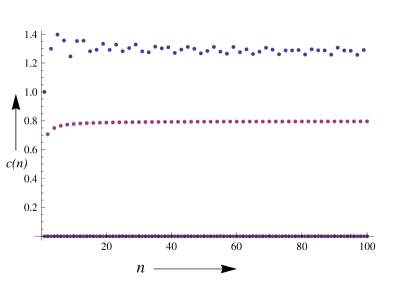
Figure 1: Plot of $c(n)$ vs $n$ for $1\leq n\leq 100$.

Fact 1

Let $f\in{\cal SB}_{n}$ be as explained in Theorem 1 towards maximizing the Walsh spectrum values at weight $w$. Then the total sum of the squares of the Walsh spectrum values at weight $w$, $\binom{n}{w}\left(rw_{f}(w)\right)^{2}$, is $\Omega(\frac{2^{2n}}{\sqrt{n}})$.

The proof of the fact seems to be quite tedious and elusive and we leave it as an open problem.

III.3 Relation between Deutsch-Jozsa algorithm and the Walsh Spectrum of Symmetric Boolean Function

Given $f$ is either constant or balanced, if the corresponding quantum implementation $U_{f}$ is available, Deutsch-Jozsa qDJ92 provided a quantum algorithm that decide in constant time which one it is. Let us now describe our interpretation of Deutsch-Jozsa algorithm in terms of Walsh spectrum values. We denote the operator for Deutsch-Jozsa algorithm as

$${\cal D}_{f}=H^{\otimes n}U_{f}H^{\otimes n},$$

where the Boolean function $f$ is available as an oracle $U_{f}$. For brevity, we abuse the notation and do not write the auxiliary qubit, i.e., $\frac{|0\rangle-|1\rangle}{\sqrt{2}}$ and the corresponding output in this case.

Now one can observe that maitra

$${\cal D}_{f}|0\rangle^{\otimes n} = \sum_{z\in\{0,1\}^{n}}\sum_{x\in\{0,1\}^{n}}\frac{(-1)^{x\cdot z\oplus f(x)}}{2^{n}}|z\rangle$$

$$= \sum_{z\in\{0,1\}^{n}}\frac{W_{f}(z)}{2^{n}}|z\rangle.$$

Note that the associated probability with a state $|z\rangle$ is $\frac{W_{f}^{2}(z)}{2^{2n}}$. Hence we have the following technical result as pointed out in maitra with our interpretation for symmetric functions.

Proposition 2

Given an $n$-variable Boolean function $f$, ${\cal D}_{f}|0\rangle^{\otimes n}$ produces a superposition of all states $z\in\{0,1\}^{n}$ with the amplitude $\frac{W_{f}(z)}{2^{n}}$ corresponding to each state $|z\rangle$. Specially, if $f\in{\cal SB}_{n}$, then the amplitude corresponding to $|z\rangle$ is $\frac{\sum_{i=0}^{n}(-1)^{f_{i}}K_{i}(wt(z),n)}{2^{n}}$.

III.4 Algorithm 1: Deutsch-Jozsa Algorithm with Special Symmetric Function

Based on the overall properties, we propose a quantum algorithm as shown in the following algorithm.

Algorithm 1
1. Choose $f\in{\cal SB}_{n}$ as explained in Theorem 1 to maximize the Walsh spectrum values at weight $w$. 2. Use the Deutsch-Jozsa algorithm to obtain a symmetric $n$-qubit state $|S^{n}\rangle=\sum\limits_{x\in\{0,1\}^{n}}a_{wt(x)}|x\rangle$, such that $\binom{n}{w}|a_{w}|^{2}$ is $\Omega(\frac{1}{\sqrt{n}})$. 3. Apply the parity measurement strategy. If the ancilla state is measured at the basis $U^{w}|\zeta\rangle$, then $|D_{w}^{n}\rangle$ is successfully obtained. Else go to Step 2 and iterate.

The following result provides the estimate of complexity of our algorithm.

Theorem 3

Let $f\in{\cal SB}_{n}$ be as explained in Theorem 1 towards maximizing the Walsh spectrum values at weight $w$. Given Fact 1, Deutsch-Jozsa algorithm produces a symmetric $n$-qubit state (before the measurement) $|S^{n}\rangle=\sum\limits_{x\in\{0,1\}^{n}}a_{wt(x)}|x\rangle$, such that $\binom{n}{w}|a_{w}|^{2}$ is $\Omega(\frac{1}{\sqrt{n}})$.

Proof: The proof follows from Theorem 1, Fact 1 and Proposition 2.  

Now the final step is to measure the symmetric state until we get the target Dicke state by using parity measurement method  (d2, , Section IIIA). Now we explain how to exploit the parity measurement in our purpose. Note (d2, , Section IIIA) assumes to use $n$ dimensional qudit ancilla, but we consider a qudit $|\zeta\rangle$ of dimension $n+1$ here. A certain unitary operator $U$ is designed such that,

$$|\zeta\rangle,U|\zeta\rangle,U^{2}|\zeta\rangle,\ldots,U^{n-1}|\zeta\rangle,U^{n}|\zeta\rangle$$

are all orthogonal to each other and $U^{n+1}|\zeta\rangle=|\zeta\rangle$. Since $|\zeta\rangle$ is an $(n+1)$-dimensional state, one can indeed obtain a set of such $n+1$ orthogonal states. The parity measurement is done on the

$$\{|\zeta\rangle,U|\zeta\rangle,U^{2}|\zeta\rangle,\ldots,U^{n}|\zeta\rangle\}$$

basis. Here $|\zeta\rangle$ is used as the target state. For the $n$-qubit control state $|x\rangle$, if it has weight $w$ then its corresponding target state, after application of this circuit, will become $U^{w}|\zeta\rangle$ (see Figure 2). Now consider an $n$-qubit symmetric state as the control input, which is $|\tau\rangle=\sum\limits_{x\in\{0,1\}^{n}}a_{w}|x\rangle,$ where $w=wt(x)$, $\sum_{i=0}^{n}\binom{n}{i}|a_{i}|^{2}=1$. After applying this circuit, one obtains $\sum\limits_{x\in\{0,1\}^{n}}a_{w}|x\rangle U^{w}|\zeta\rangle$. Thus, if one measures in

$$\{|\zeta\rangle,U|\zeta\rangle,U^{2}|\zeta\rangle,\ldots,U^{n}|\zeta\rangle\}$$

basis, then the state $|D_{w}^{n}\rangle$ will be obtained when the measurement result of the ancilla state is $U^{w}|\zeta\rangle$.

Figure 2: Generalized Parity Module as in (d2, , Fig. 1). If $wt(x)=w$, then the ancilla will become $U^{w}|\zeta\rangle$.

Since the probability of target Dicke state is $\Omega(\frac{1}{\sqrt{n}})$, we should repeat the whole procedure at most $O(\sqrt{n})$.

Example 2

Let us have an example taking $n=6,w=2$ to outline our method. In this case the Dicke state will be

$$|D^{6}_{2}\rangle=\sum\limits_{x\in\{0,1\}^{6},wt(x)=2}\frac{1}{\sqrt{15}}|x\rangle.$$

We start with is an $n=6$ variable symmetric Boolean function having Walsh spectrum value at each of the weight $w=2$ point as $12$ (following Theorem 1, one may refer to Example 1 also). There are $\binom{n}{w}=\binom{6}{2}=15$ such points. The amplitude associated with each point after the DJ algorithm is $\frac{12}{2^{6}}=\frac{3}{16}$. Thus we get $\sum_{x\in\{0,1\}^{6},wt(x)=2}\frac{3}{16}|x\rangle+\sum_{x\in\{0,1\}^{6},wt(x)\neq 2}a_{x}|x\rangle$ initially. Thus, the probability associated with $|D^{6}_{2}\rangle$ will be $\binom{6}{2}(\frac{3}{16})^{2}=\frac{135}{256}=0.52734375$ and hence one may note that the probability that, after parity measurement, it will land into $|D^{6}_{2}\rangle$ is quite high.

III.5 Comparison with a Previous Method

It was explained in d2 how one can obtain $|D^{n}_{w}\rangle$ from $\frac{1}{2^{\frac{n}{2}}}\sum_{x\in\{0,1\}^{n}}|x\rangle$. However, the idea explained in (d2, , Section IIIA) works efficiently only for $w=\lceil\frac{n}{2}\rceil$ or $\lfloor\frac{n}{2}\rfloor$. The most general work in this direction has appeared in dickold where biased Hadamard transformation was exploited. The strategy of dickold uses biased Hadamard transformation

$$\begin{pmatrix}\sqrt{1-\frac{w}{n}}&\sqrt{\frac{w}{n}}\\ \sqrt{\frac{w}{n}}&-\sqrt{1-\frac{w}{n}}\end{pmatrix}^{\otimes n}$$

on $|0\rangle^{\otimes n}$ such that the probability associated with $|D^{n}_{w}\rangle$ will be $\binom{n}{w}(\frac{w}{n})^{w}(1-\frac{w}{n})^{n-w}\geq\sqrt{\frac{2}{n\pi}}$, i.e., $\Omega(\frac{1}{\sqrt{n}})$. Thus, the probability of our case and also in dickold are of the same order. While the theoretical comparison of the exact probability values seems elusive, we have made detailed enumerations to observe that the exact probability values in our case are better than that of dickold . Below we present enumeration results towards that.

First we present two graphs to show the probability values associated to $|D^{n}_{w}\rangle$ for all $w$, when $n=999$ (to represent odd case) or $1000$ (to represent even case). For our case, it is $\binom{n}{w}\frac{(\sum_{i=0}^{n}|K_{i}(w,n)|)^{2}}{2^{2n}}$ (after application of Deutsch-Jozsa algorithm without measurement), and for the case of dickold it is $\binom{n}{w}(\frac{w}{n})^{w}(1-\frac{w}{n})^{n-w}$ (after application of biased Hadamard transform). From Figure 3 and Figure 4, it is clear to note that our method provides higher probability (the upper curve) in all the cases except $w=0,n$ (which are trivial ones) and $w=\frac{n}{2}$ for $n=1000$.

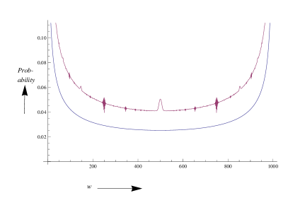
Figure 3: Plot of probabilities associated with $|D^{n}_{w}\rangle$ against $w$ in our case (above) and in dickold (below) for $n=999$.

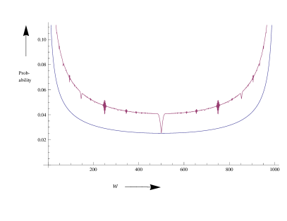
Figure 4: Plot of probabilities associated with $|D^{n}_{w}\rangle$ against $w$ in our case (above) and in dickold (below) for $n=1000$.

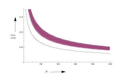
Figure 5: Plot of probabilities associated with $|D^{n}_{w}\rangle$ against $n$ in our case (above) and in dickold (below) for $n=4$ to $1000$ and $w=\lfloor\frac{n}{4}\rfloor$.

In both figures, the present algorithm shows some variation of probability when the weight is around $\lfloor\frac{n}{4}\rfloor$. To check whether or not these cases still shows the higher probability than the previous method, we look into the $w=\lfloor\frac{n}{4}\rfloor$ case a little bit more. From Figure 5, one may note that our probability values (the upper curve) are higher than the case of dickold . These results explains the advantage of the use of a suitable symmetric Boolean function which shows higher Walsh spectrum values for the given weight.

III.6 Algorithm 2: Additional Improvement by exploiting biased Hadamard Operator

We have provided numerical evidences that using proper symmetric Boolean functions in Deutsch-Jozsa algorithm provides better probability than the use of biased Hadamard transform as described in dickold . However, motivated by dickold , a natural extension should be to couple biased Hadamard transform in Deutsch-Jozsa algorithm instead of (unbiased) Hadamard transform. Thus, let us refer to the general description of a Hadamard type transformation (biased or unbiased) that can be written as $B_{r,n}=\begin{pmatrix}\sqrt{1-\frac{r}{n}}&\sqrt{\frac{r}{n}}\\ \sqrt{\frac{r}{n}}&-\sqrt{1-\frac{r}{n}}\end{pmatrix}$. We will replace the standard notation of $w$ here by $r$ as we will not restrict ourselves to integer values $w\in[0,\ldots,n]$, but use any real number $r\in[0,n]$ to obtain the optimum probability of success to get a Dicke state.

Instead of using the operator ${\cal D}_{f}=H^{\otimes n}U_{f}H^{\otimes n}$, let us first describe the most general operator of the form

$${\cal D^{\prime}}_{f}=B_{r_{1},n}^{\otimes n}U_{f}B_{r_{2},n}^{\otimes n},$$ (1)

where $r_{1},r_{2}$ are real numbers in $[0,n]$.

First, we consider the case when $r_{1}=\frac{n}{2}$, i.e., $B_{r_{1},n}=H$, but $r_{2}=r$ varies towards optimization. That is

$${\cal D^{\prime}}_{f}=H^{\otimes n}U_{f}B_{r,n}^{\otimes n}.$$ (2)

One may note that the application of ${\cal D^{\prime}}_{f}$ on $|0\rangle^{\otimes n}$ will produce

${\cal D^{\prime}}_{f}|0\rangle^{\otimes n}=\frac{1}{\sqrt{2^{n}}}\sum_{z\in\{0,1\}^{n}}$

$\left(\sum_{x\in\{0,1\}^{n}}(-1)^{x\cdot z\oplus f(x)}(1-\frac{r}{n})^{\frac{n-d(x,z)}{2}}(\frac{r}{n})^{\frac{d(x,z)}{2}}\right)|z\rangle$, where $d(x,z)$ is the (Hamming) distance between two same length binary strings $x$ and $z$. Before proceeding further, we also have the following technical result.

Proposition 3

Let ${\cal D^{\prime}}_{f}=H^{\otimes n}U_{f}B_{r,n}^{\otimes n}$. If $f\in{\cal SB}_{n}$ then ${\cal D^{\prime}}_{f}|0\rangle^{\otimes n}$ is a symmetric state.

Proof: We need to prove that $\sum_{x\in\{0,1\}^{n}}(-1)^{x\cdot z\oplus f(x)}(1-\frac{r}{n})^{\frac{n-d(x,z)}{2}}(\frac{r}{n})^{\frac{d(x,z)}{2}}$ is same for all the $z\in\{0,1\}^{n}$ having the same Hamming weight. Let us consider $u,v\in\{0,1\}^{n}$ such that $u\neq v$, but $wt(u)=wt(v)$. Then we need to prove that $\sum_{x\in\{0,1\}^{n}}(-1)^{x\cdot u\oplus f(x)}(1-\frac{r}{n})^{\frac{n-d(x,u)}{2}}(\frac{r}{n})^{\frac{d(x,u)}{2}}$ $=$ $\sum_{x\in\{0,1\}^{n}}(-1)^{x\cdot v\oplus f(x)}(1-\frac{r}{n})^{\frac{n-d(x,v)}{2}}(\frac{r}{n})^{\frac{d(x,v)}{2}}$.

The proof follows from the fact that $\sum_{x\in\{0,1\}^{n},wt(x)=w}(-1)^{x\cdot u\oplus f(x)}(1-\frac{r}{n})^{\frac{n-d(x,u)}{2}}(\frac{r}{n})^{\frac{d(x,u)}{2}}=$ $\sum_{x\in\{0,1\}^{n},wt(x)=w}(-1)^{x\cdot v\oplus f(x)}(1-\frac{r}{n})^{\frac{n-d(x,v)}{2}}(\frac{r}{n})^{\frac{d(x,v)}{2}}$, given that $f$ is symmetric.  

The main problem in this case is that we need to go for trial and error by modifying the symmetric Boolean functions and trying out different values of $\frac{r}{n}$. So far, we could not obtain the exact characterization of symmetric functions while biased Hadamard transform is used. Based on this, we propose Algorithm 2 as follows.

Algorithm 2
1. Apply ${\cal D^{\prime}}_{f}$ to $|0\rangle^{\otimes n}$ to obtain a symmetric $n$-qubit state. The value of $\frac{r}{n}$ and the choice of the symmetric Boolean functions are achieved heuristically. 2. Use parity measurement strategy. If the ancilla state is measured at the basis $U^{w}|\zeta\rangle$, then $|D_{w}^{n}\rangle$ is successfully obtained. Else take the parameters as in Step 1 once again and iterate Step 2.

As we could not characterize this, to provide some experimental results in this direction (see Table 1 at the end of this draft), we used the following method for some small values of $n$ ($n=4$ to $9$). We select each of the Boolean functions $f$ from ${\cal SB}_{n}$. Given $f$ and a specific weight $w$, $1\leq w\leq n$, we write the expression of success probability as a function of $r$. Then we apply the $Maximize$ function available in $Mathematica$ $8.0$ to compute the optimum value of $r$ given $f,w$, so that the success probability becomes maximum. Note that, as we could not characterize the process yet, this is an exhaustive task and for each $n$, it requires checking of $2^{n+1}$ symmetric Boolean functions. That is the reason, we can study it for only a few small values of $n$. However, this is a classical computation that can be done as an off-line work. Once such programs are executed, we can have a database of proper ${f\in\cal SB}_{n}$ and the corresponding $r$ to have the optimal success probability to obtain $|D^{n}_{w}\rangle$. Given these data, the actual quantum algorithm to obtain Dicke states can be efficiently implemented.

IV Numerical Comparison of Three Approaches

Now we compare three approaches:

• using biased Hadamard operator as shown in dickold ,

• Algorithm 1 based on ${\cal D}_{f}|0\rangle^{\otimes n}$, and

• Algorithm 2 based on ${\cal D^{\prime}}_{f}|0\rangle^{\otimes n}$.

The first two cases need $O(\sqrt{n})$ complexity, and the third one is a heuristic that shows improved results than the first two. Some numerical results of the probability associated with $|D^{n}_{w}\rangle$ are shown in Table 1 at the end of this draft for $n=4,\cdots,9$. As shown in the table, we note that Algorithm 2 provides the highest probability than others. There are a few interesting observations from the enumeration results.

• We note that the improvements using ${\cal D^{\prime}}_{f}$ are highly significant at $w=\lfloor\frac{n}{2}\rfloor$ or $\lceil\frac{n}{2}\rceil$ and the significance reduces as $w$ moves away from the middle, i.e., towards $w=1$ or $n-1$.

• In case of using ${\cal D^{\prime}}_{f}$, the success probabilities at $w$ and $n-w$ weights are same for all the values of $w$, i.e., $w\geq 1$. However, the values of $r$ in those cases are same at $w$ and $n-w$ weights for $w\geq 2$ only.

V The complete strategy using Grover Algorithm

Quadratic improvement by Grover’s algorithm qGR96 is achieved in several applications. We point out here how that can be exploited in our algorithm. Although we can construct the target Dicke state by measuring the intermediate quantum state, we may increase the efficiency further by using the amplitude amplification method. Based on this, an adiabatic evolution has been used towards amplitude amplification of the desired states in dickold , but no complexity analysis was shown. In this work, instead, we apply the conventional Grover algorithm qGR96 as it provides a quadratic speed-up.

Instead of equal superposition $|\psi\rangle=H^{\otimes n}|0\rangle^{\otimes n}=\frac{1}{2^{\frac{n}{2}}}\sum_{x\in\{0,1\}^{n}}|x\rangle$ in Grover algorithm, we will use the symmetric state of the form $|\Psi\rangle={\cal D}_{f}(|0\rangle^{\otimes n})=\sum_{x\in\{0,1\}^{n}}\frac{W_{f}(x)}{2^{n}}|x\rangle$ exploiting the properly chosen Boolean function $f(x)$, as explained in the previous sections.

Further, towards inverting the phase, we will use another symmetric Boolean function $g(x)$, different from $f(x)$, where $g(x)=1$, when $wt(x)=w$, and $g(x)=0$, otherwise. Based on $g(x)$, we implement the inversion operator as ${\cal O}_{g}$, that inverts the phase of the states $|x\rangle$ where $\{x\in\{0,1\}^{n}\,|wt(x)=w\}$. Thus, we consider the operator

$$G_{t}=\left[(2|\Psi\rangle\langle\Psi|-I){\cal O}_{g}\right]^{t}$$

on $|\Psi\rangle$ to get $|\Psi_{t}\rangle$.

Consider the $n$-qubit state $|\Psi\rangle=\sum_{s\in S}u_{s}|s\rangle+\sum_{s\in\{0,1\}^{n}\setminus S}v_{s}|s\rangle$, where $u_{s},v_{s}$ are real and $\sum_{s\in S}u^{2}_{s}+\sum_{s\in\{0,1\}^{n}\setminus S}v^{2}_{s}=1$. For brevity, let us represent $|\Psi\rangle=\sum\limits_{s\in S}u_{s}|s\rangle+\sum\limits_{s\in\{0,1\}^{n}\setminus S}v_{s}|s\rangle=u|X\rangle+v|Y\rangle$. That is, $u^{2}=\sum\limits_{s\in S}u^{2}_{s}$ and $v^{2}=\sum\limits_{s\in\{0,1\}^{n}\setminus S}v^{2}_{s}$.

Let $u=\sin\theta$, $v=\cos\theta$. It is easy to check that the application of $[(2|\Psi\rangle\langle\Psi|-I){\cal O}_{g}]^{t}$ operator on $|\Psi\rangle$ produces $|\Psi_{t}\rangle$, in which the probability amplitude of $|X\rangle$ is $\sin(2t+1)\theta$.

We will now use such states $|\Psi_{t}\rangle$ in parity measurement. Consider that after the Deutsch-Jozsa algorithm we obtain a symmetric $n$-qubit state (before the measurement)

$$|S^{n}\rangle=\sum\limits_{x\in\{0,1\}^{n}}a_{wt(x)}|x\rangle,$$

such that $\binom{n}{w}|a_{w}|^{2}=\frac{c}{\sqrt{n}}$, for some constant $c$. Thus, we have the initial amplitude of target states, $\{x\in\{0,1\}^{n}\,|wt(x)=w\}$, is $\sin\theta=\binom{n}{w}|a_{w}|=\sqrt{\frac{c}{\sqrt{n}}}$. For large $n$, one can approximate it as $\theta=\frac{\sqrt{c}}{\sqrt[4]{n}}$ and hence we need $t$ iterations of Grover like strategy such that $(2t+1)\theta\approx\frac{\pi}{2}$, i.e., $t\approx\frac{\pi\sqrt[4]{n}}{2\sqrt{c}}$.

Here we have good (almost exact) estimate of $t$, which is not known priori for application in search algorithms. After the application of Grover like strategy, we will get another symmetric $n$-qubit state $|T^{n}\rangle=\sum\limits_{x\in\{0,1\}^{n}}a^{\prime}_{wt(x)}|x\rangle$ such that $\binom{n}{w}|a^{\prime}_{w}|^{2}$ will be very close to $1$ and the parity measurement will produce $|D^{n}_{w}\rangle$ mostly in one step with very high probability. Thus the exact strategy is similar to Algorithm 1 (Algorithm 2 can be modified with a similar way) in the previous section, where we add one more step as follows.

Algorithm 3
1. Let $f\in{\cal SB}_{n}$ be as explained in Theorem 1 to maximize the Walsh spectrum values at weight $w$. 2. Use any of the above three strategies (our strategies exploiting Hadamard or biased Hadamard transform or the strategy of dickold ) to obtain a symmetric $n$-qubit state $|S^{n}\rangle=\sum\limits_{x\in\{0,1\}^{n}}a_{wt(x)}|x\rangle$, such that $\binom{n}{w}|a_{w}|^{2}$ is $\Omega(\frac{1}{\sqrt{n}})$. 3. Use $G_{t}$ on $|S^{n}\rangle$, $t$ many times, where $t$ is $O(\sqrt[4]{n})$ to obtain $|T^{n}\rangle=\sum\limits_{x\in\{0,1\}^{n}}a^{\prime}_{wt(x)}|x\rangle$ such that $\binom{n}{w}|a^{\prime}_{w}|^{2}$ is very close to $1$. 4. Use parity measurement strategy. If the ancilla state is measured at the basis $U^{w}|\zeta\rangle$, then $|D_{w}^{n}\rangle$ is successfully obtained. Else go to Step 2 and iterate.

We need $O(\sqrt[4]{n})$ steps using Grover algorithm in each run and then a parity measurement should provide $|D_{w}^{n}\rangle$. Thus, we get a quadratic speed-up (which is quite natural) over just using Deutsch-Jozsa algorithm. The number of parity measurement was $O(\sqrt{n})$ in the earlier case, once in each iteration. Here it is only a very few (may be 1 in most of the cases).

VI Conclusion and Open Problems

In this work, we study several quantum algorithms to construct arbitrary Dicke state in a disciplined manner. The key idea is to find a suitable symmetric Boolean function for Deutsch-Jozsa algorithm for the given $n$ and $w$, use of the Grover algorithm and the generalized parity measurement strategy. Further, we show that it is possible to obtain improved results using biased Hadamard transform suitably. Our results improve the probabilities obtained in dickold and thus provide faster method to construct Dicke states. The problem open in this area is to characterize the enumeration results in case of modifying the Deutsch-Jozsa algorithm with biased Hadamard transform. Obtaining the exact bias ($\frac{r}{n}$) in biased Hadamard transform with the corresponding symmetric function to optimize the probability corresponding to the Dicke state seems to be an interesting problem.

Though we look at the problem from theoretical angle, the algorithmic blocks used by us have experienced major advancement towards actual implementation. One may refer to (qNC02, , Section 7) for literature related to implementation of quantum gates as well as Deutsch-Jozsa algorithm, Grover algorithm and several measurement techniques. As example, the idea of implementing biased Hadamard transform is related to the Fabry-Perot cavity (qNC02, , Page 299).

Acknowledgments: The authors like to thank Prof. A. M. Childs for providing critical comments on an initial version of this paper and pointing to dickold .

$n\downarrow$	$w\rightarrow$	1	2	3	4	5	6	7	8
4	${\cal D^{\prime}}_{f}|0\rangle^{\otimes n}$	0.833609	0.981763	0.833609	–	–	–	–	–
	$f$	01	02	05	–	–	–	–	–
	$r$	0.468136	0.298698	0.468136	–	–	–	–	–
	${\cal D}_{f}|0\rangle^{\otimes n}$	0.5625	0.375	0.5625	–	–	–	–	–
	dickold	0.421875	0.375	0.421875	–	–	–	–	–
5	${\cal D^{\prime}}_{f}|0\rangle^{\otimes n}$	0.748304	0.92852	0.92852	0.748304	–	–	–	–
	$f$	03	02	05	16	–	–	–	–
	$r$	1.42458	0.313077	0.313077	3.57542	–	–	–	–
	${\cal D}_{f}|0\rangle^{\otimes n}$	0.703125	0.625	0.625	0.703125	–	–	–	–
	dickold	0.4096	0.3456	0.3456	0.4096	–	–	–	–
6	${\cal D^{\prime}}_{f}|0\rangle^{\otimes n}$	0.730278	0.823495	0.954987	0.823495	0.730278	–	–	–
	$f$	03	02	05	0A	29	–	–	–
	$r$	1.48129	0.357282	0.277975	0.357282	4.51871	–	–	–
	${\cal D}_{f}|0\rangle^{\otimes n}$	0.585938	0.527344	0.3125	0.527344	0.585938	–	–	–
	dickold	0.401878	0.329218	0.3125	0.329218	0.401878	–	–	–
7	${\cal D^{\prime}}_{f}|0\rangle^{\otimes n}$	0.704306	0.754753	0.907588	0.907588	0.754753	0.704306	–	–
	$f$	07	60	05	0A	53	4A	–	–
	$r$	2.44507	5.93733	0.27984	0.27984	5.93733	2.44507	–	–
	${\cal D}_{f}|0\rangle^{\otimes n}$	0.683594	0.512695	0.546875	0.546875	0.512695	0.683594	–	–
	dickold	0.396569	0.318745	0.293755	0.293755	0.318745	0.396569	–	–
8	${\cal D^{\prime}}_{f}|0\rangle^{\otimes n}$	0.698181	0.710643	0.813922	0.92625	0.813922	0.710643	0.698181	–
	$f$	3F	C0	BF	A0	AF	AC	AD	–
	$r$	5.51859	6.91248	7.69903	7.74472	7.69903	6.91248	5.51859	–
	${\cal D}_{f}|0\rangle^{\otimes n}$	0.598145	0.553711	0.413574	0.273438	0.413574	0.553711	0.598145	–
	dickold	0.392696	0.311462	0.281632	0.273438	0.281632	0.311462	0.392696	–
9	${\cal D^{\prime}}_{f}|0\rangle^{\otimes n}$	0.684842	0.651002	0.76886	0.884277	0.884277	0.76886	0.651002	0.684842
	$f$	0F	180	0D	140	15F	6A	153	16A
	$r$	3.4566	7.86171	0.858163	8.7469	8.7469	0.858153	7.86171	3.4566
	${\cal D}_{f}|0\rangle^{\otimes n}$	0.672913	0.430664	0.415283	0.492188	0.492188	0.415283	0.430664	0.672913
	dickold	0.389744	0.306102	0.273129	0.260182	0.260182	0.273129	0.306102	0.389744

Table 1: Probability values using biased Hadamard transform (in this case we provide the corresponding symmetric function $f$ represented as a hexadecimal number of the $(n+1)$ length bit-string $f_{n},f_{n-1},\ldots,f_{1},f_{0}$ and the value of $r$), using (standard) Hadamard transform and the method of dickold .

References

- (1) A. M. Childs, E. Farhi, J. Goldstone and S. Gutmann. Finding cliques by quantum adiabatic evolution. Quantum Information and Computation 2, 181 (2002). Available at http://arxiv.org/abs/quant-ph/0012104.
- (2) A. Chiuri, C. Greganti, M. Paternostro, G. Vallone, and P. Mataloni. Experimental Quantum Networking Protocols via Four-Qubit Hyperentangled Dicke States. Physical Review Letters 109, 173604 (2012).
- (3) E. Demenkov, A. Kojevnikov, A. Kulikov and G. Yaroslavtsev. New upper bounds on the Boolean circuit complexity of symmetric functions. Information Processing Letters 110, 264-267 (2010).
- (4) D. Deutsch and R. Jozsa. Rapid solution of problems by quantum computation. Proceedings of Royal Society of London A 439, 553-558 (1992).
- (5) R. H. Dicke. Coherence in Spontaneous Radiation Processes. Physical Review 93(1), 99 (1954).
- (6) P. Feinsiver and R. Fitzgerald. The Spectrum of Symmetric Krawtchouk Matrices. Linear Algebra & Applications 235, 121-139 (1996).
- (7) P. Feinsilver and J. Kocik. Krawtchouk matrices from classical and quantum random walks. Contemporary Mathematics 287, 83-96 (2001).
- (8) L. Grover. A fast quantum mechanical algorithm for database search. In Proceedings of 28th Annual Symposium on the Theory of Computing, 212-219 (1996). Available at http://xxx.lanl.gov/abs/quant-ph/9605043.
- (9) R. Ionicioiu, A. E. Popescu, W. J. Munro and T. P. Spiller. Generalized parity measurements. Physical Review A 78, 052326 (2008).
- (10) N. Kiesel, C. Schmid, G. Toth, E. Solano, and H. Weinfurter. Experimental Observation of Four-Photon Entangled Dicke State with High Fidelity. Physical Review Letters 98, 063604 (2007).
- (11) I. Krasikov. On integral zeros of Krawtchouk polynomials. Journal of Combinatorial Theory, Series A 74, 71-99 (1996).
- (12) J. Li, K. Chalapat, and G. S. Paraoanu. Entanglement of superconducting qubits via microwave fields: classical and quantum regimes. Physical Review B 78, 064503 (2008)
- (13) I. E. Linington and N. V. Vitanov. Decoherence-free preparation of Dicke states of trapped ions by collective stimulated Raman adiabatic passage. Physical Review A 77, 062327 (2008).
- (14) F. J. MacWillams and N. J. A. Sloane. The Theory of Error Correcting Codes. North Holland, 1977.
- (15) S. Maitra and P. Mukhopadhyay. Deutsch-Jozsa Algorithm Revisited in the Domain of Cryptographically Significant Boolean Functions. In International Journal on Quantum Information 3(2), 359-370 (2005).
- (16) M. A. Nielsen and I. L. Chuang, Quantum Computation and Quantum Information, Cambridge University Press, 2010.
- (17) R. Prevedel, G. Cronenberg, M. S. Tame, M. Paternostro, P. Walther, M. S. Kim, and A. Zeilinger. Experimental Realization of Dicke States of up to Six Qubits for Multiparty Quantum Networking. Physical Review Letters 103, 020503 (2009).
- (18) S. Sarkar and S. Maitra. Efficient search for symmetric Boolean functions under constraints on Walsh spectra values. Journal of Combinatorial Mathematics and Combinatorial Computing 68, 163-191 (2009).
- (19) W. Wieczorek, R. Krischek, N. Kiesel, P. Michelberger, G. Toth, and H. Weinfurter. Experimental Entanglement of a Six-Photon Symmetric Dicke State. Physical Review Letters 103, 020504 (2009).