The distribution of faint satellites around central galaxies in the CFHT Legacy Survey

Abstract

We investigate the radial number density profile and the abundance distribution of faint satellites around central galaxies in the low redshift universe using the CFHT Legacy Survey. We consider three samples of central galaxies with magnitudes of $M_{\rm r}=-21$, $-22$, and $-23$ selected from the Sloan Digital Sky Survey (SDSS) group catalog of Yang et al.. The satellite distribution around these central galaxies is obtained by cross-correlating these galaxies with the photometric catalogue of the CFHT Legacy Survey. The projected radial number density of the satellites obeys a power law form with the best-fit logarithmic slope of $-1.05$, independent of both the central galaxy luminosity and the satellite luminosity. The projected cross correlation function between central and satellite galaxies exhibits a non-monotonic trend with satellite luminosity. It is most pronounced for central galaxies with $M_{\rm r}=-21$, where the decreasing trend of clustering amplitude with satellite luminosity is reversed when satellites are fainter than central galaxies by more than 2 magnitudes. A comparison with the satellite luminosity functions in the Milky Way and M31 shows that the Milky Way/M31 system has about twice as many satellites as around a typical central galaxy of similar luminosity. The implications for theoretical models are briefly discussed.

1. Introduction

The distribution of satellite galaxies around the central galaxy in a dark matter halo carries important information for the underlying cosmology, dark matter properties and galaxy formation processes. It is specified by the abundance distribution of satellites with varying properties (luminosity, color, star formation rate and so on), and the spatial distribution of the satellites. A clear picture of how satellite galaxies are distributed in the real universe provides a critical test for the theoretical models of cosmology and galaxy formation.

Current N-body studies have shown that the abundance of subhalos that satellites inhabit is nearly scale invariant, if the subhalo mass scaled by the virial mass of the host halo is considered (Madau et al., 2008; Angulo et al., 2009; Han et al., 2011). However, due to the complex baryonic physics involved in galaxy formation, the relation between the dark matter mass of a halo and its central galaxy mass is not linear (e.g. Yang et al., 2003; Tinker et al., 2005; Mandelbaum et al., 2006; Wang et al., 2006; Yang et al., 2007; Zheng et al., 2007; Guo et al., 2010; Moster et al., 2010; Wang & Jing, 2010; More et al., 2011; Li et al., 2012). Furthermore, when a galaxy together with its surrounding halo infalls into a bigger halo and becomes a satellite, physical processes such as tidal stripping, ram pressure and gas starvation begin to take effects, which further complicates the galaxy-subhalo relation. Thus, the satellite distribution can not be inferred from the subhalo distribution nontrivially, and observations of the satellite distribution are expected to provide important clues to these physical processes.

From rich clusters to Milky Way (MW)-sized groups, the luminosity of central galaxies changes by $\sim 1$ order of magnitude, while the mass of their host halos spans $\sim 3$ orders of magnitude. The luminosity-halo mass relation flattens at the massive halo end, as a result of lower efficiency of converting baryonic matter to light in more massive halos. We then expect that the number of satellites with fixed magnitude difference between the satellite and the central galaxy ($\Delta m=M^{s}-M^{c}$) is larger for more luminous central galaxies, unlike the nearly scale-independent behavior in the subhalo population.

The Local Group satellites, due to their proximity, have been observed in the most detail, and the observational data has been used to test and calibrate various galaxy formation models. The apparent tension between the large number of subhalos in $\Lambda$CDM simulations and only dozens of satellites observed in the Local Group has challenged theorists, making them either scrutinize various baryonic processes that might suppress star formation in small halos (Kravtsov et al., 2004; Koposov et al., 2009), or investigate the possibility of alternative dark matter models (Zavala et al., 2009; Lovell et al., 2012).

Despite possible underpopulation of the satellites as a whole in the Milky Way compared with theoretical subhalos, some authors have found that the existence of the two Magellanic Clouds (MCs) seems incompatible with the $\Lambda$CDM universe. Koposov et al. (2009) found that it is very difficult to reproduce the Magellanic Clouds in models that can solve the ’missing satellite’ problem. Under the assumption of abundance matching, Boylan-Kolchin et al. (2010) stated that there is only a $10\%$ chance of finding two galaxies as bright as Magellanic Clouds in a halo of virial mass $M_{\rm vir}=10^{12}{\rm M_{\odot}}$. Busha et al. (2011) reached a similar conclusion also with an abundance matching method. They showed that, even before the abundance matching is applied, the probability of hosting two satellites with maximum circular velocity exceeding $v_{\max}=50\,{\rm{km\,s^{-1}}}$ which is the lower bound of Magellanic Clouds (van der Marel et al., 2002; Stanimirović et al., 2004) is only $\sim 8\%$ for halos of $M_{\rm vir}=1.2\times 10^{12}{\rm M_{\odot}}$ in their simulation. This probability increases to $\sim 20\%$ for halos of $M_{\rm vir}=2.6\times 10^{12}{\rm M_{\odot}}$. However, it is contradictory to the result of Wang et al. (2012), in which the number of subhalos having $v_{\rm max}>60\,{\rm{km\,s^{-1}}}$ in halos with $M_{\rm vir}=2.6\times 10^{12}{\rm M_{\odot}}$ is already over $1$. They found that the number of subhalos above the maximum circular velocity threshold can be underestimated if the mass resolution of simulation is not high enough. The fact that the number of particles within the virial radius in Busha et al. (2011) is smaller than the minimum number needed to achieve convergence as listed in Wang et al. (2012) may account for part of the difference in the probability of finding two subhalos like Magellanic Clouds.

On the other hand, it is doubted that the Milky Way, as a single case, may be representative of galaxies with a comparable luminosity. Some recent works have been dedicated to statistical measurements of satellite abundance in large scale surveys. Guo et al. (2011) studied the luminosity function of satellites around isolated primaries in the Sloan Digital Sky Survey (SDSS; York et al., 2000), finding that the number of satellites brighter than $M_{\rm v}=-14$ in MW/M31-like galaxies is lower than that in MW/M31 by a factor of 2. Nierenberg et al. (2012) used imaging and photometric redshift catalogs from the COSMOS survey to model the satellite distributions. Their accumulated luminosity function of satellites in MW-luminosity hosts is consistent with that in Guo et al. (2011). Robotham et al. (2012) searched for the Milky Way-Magellanic Clouds analogues in the Galaxy and Mass Assembly (GAMA) survey, finding that only $3.4\%$ of MW mass galaxies have two companions at least as massive as the small Magellanic Cloud, and only $0.4\%$ have an analogous MW-MCs system if these galaxies are all restricted to be late-type and star-forming.

The spatial distribution of satellite galaxies builds upon that of subhalos. Many physical processes that affect the luminosity-halo mass relation are dependent on the cluster/group-centric radius. Therefore, the radial distribution of satellite galaxies provides indispensable information of various processes that have shaped the luminosity-halo mass relation. $\Lambda$CDM simulations have confirmed that subhalos are distributed less centrally concentrated in the host halo than the dark matter, exhibiting a central core in the radial distribution of their number density (Diemand et al., 2004; Gao et al., 2004; Ludlow et al., 2009; Gao et al., 2012). In addition, the number density profile of subhalos has been shown to have a similar shape over a wide mass range. The radial distribution of satellite galaxies, on the other hand, is usually described by a power law, $\Sigma(r_{\rm p})\sim{r_{\rm p}}^{\rm\alpha}$, where $\Sigma(r_{\rm p})$ is the projected number density of satellites measured in observations. However, no consensus has been reached regarding the power law index $\alpha$ which spans a wide range from -0.5 to -1.7 (Madore et al., 2004; Smith et al., 2004; Sales & Lambas, 2005; Chen et al., 2006). Recent work has taken advantage of the large data sample from surveys like SDSS and COSMOS to study the satellite radial distribution. Chen et al. (2006) used the SDSS spectroscopic sample to study the projected radial distribution of satellites around isolated $L^{\ast}$ galaxies, constraining the power law slope to be $-1.7$. Watson et al. (2010) modeled the clustering of luminous red galaxies in SDSS in the framework of halo occupation distribution (HOD). They found that on projected scales $0.016\,h^{-1}{\rm{Mpc}}\leq r_{\rm p}\leq 0.42\,h^{-1}{\rm{Mpc}}$, the radial density profile of luminous red galaxies is close to an isothermal distribution. Nierenberg et al. (2012) detected satellites up to eight magnitude fainter than their host galaxies (with stellar mass above $10^{10.5}{\rm M_{\odot}}$) by subtracting the host light profile in the COSMOS survey. They constructed parametrized models for the satellite spatial distribution, number of satellites per host, and background galaxies, and then inferred the parameters using Markov Chain Monte Carlo (MCMC) method. The power law slope was found to be $-1.1$, independent of host stellar mass and satellite luminosities.

Observational studies mentioned above have either used a spectroscopic sample, or combined a spectroscopic sample for central galaxies with a deeper photometric sample to probe fainter satellites. In the latter case, the background must be subtracted properly due to the lack of redshift information. So far, several background subtraction methods have been used. For example, Lares et al. (2011) applied a color cut, $g-r<1$, to identify satellite galaxies, taking galaxies with colors beyond this range as background galaxies for the redshift range they considered. However, this method failed at $r_{\rm p}<100$ ${\rm{kpc}}$. Guo et al. (2011) counted the number of galaxies in an annuli 300 ${\rm{kpc}}<r_{\rm p}<600$ ${\rm{kpc}}$ to estimate the background. Nierenberg et al. (2012) used a similar method to build a prior in modeling the background. Liu et al. (2011) randomized the host positions on the sky and searched for projected companions from the background. They excluded galaxies with photometric redshift $z_{\rm p}>0.23$ in the whole calculation to lower the noise, and then corrected for this photo-z loss and for the under-deduction of background.

In this work, we use the halo-based group catalog of the SDSS constructed by Yang et al. (2007) to optimize the selection of central galaxies. We use a deep photometric catalog of the CFHT Legacy Survey, which is $\sim$ 3 magnitude deeper than the SDSS, to provide reliable information about the faint satellite galaxies around the central ones. Furthermore, we adopt a novel method of background subtraction that does not rely on models of the local environment or the photometric redshift information. Thus we are able to produce a reliable measurement of the satellite abundance and the radial density distribution for central galaxies as bright as or brighter than the Milky Way.

The remaining sections are arranged as follows. Our methodology is described in section 2, along with the dataset and sample selection. Results of the radial distributions and the abundance of satellites are presented in sections 3 $\&$ 4. Conclusions are given in section 5. Throughout this paper, we assume a $\Lambda$CDM cosmology with $\Omega_{\rm m}=0.3$, $\Omega_{\rm\Lambda}=0.7$, and $H_{\rm 0}=100h\,{\rm{km\,s^{-1}}}{\rm Mpc}^{-1}$ with $h=0.7$. All magnitudes are given in the AB system.

2. Data and Methods

2.1. Data

The data used in this work is based on the photometric catalogue of the CFHT Legacy Survey (Gwyn, 2011). The wide fields of the survey consist of 171 square degree pointings, which is about 145 ${\rm deg}^{2}$ when the masked areas are excluded. The star-galaxy separation is done based on the Spectral Energy Distribution (SED) fitting and on the source size, closely following the method adopted by Coupon et al. (2009). The survey adopts a 5-band photometric system ($u^{\ast},g^{\prime},r^{\prime},i^{\prime},z^{\prime}$), with a limiting magnitude of $r^{\prime}=25.9$. To ensure a high photometric accuracy, we select galaxies with $r^{\prime}<23.0$ to be the photometric sample from which satellites are searched for. In what follows, we omit the prime when referring to the absolute magnitude in $r^{\prime}$ band which will be written as $M_{\rm r}$.

We build our sample of central galaxies using the group catalogue constructed by Yang et al. (2007). Their extracted galaxy catalog is based on the NYU-VAGC (Blanton et al., 2005) which is selected from the SDSS (York et al., 2000) data release 7 (DR7; Abazajian et al. 2009), and supplemented with additional redshifts (e.g. from 2dF) to compensate for the untargeted galaxies due to fiber collisions. The resulting number of galaxy groups identified is about $4.7\times 10^{5}$, with spectroscopic redshifts $0.01<z<0.2$. After removing groups near the edges of the survey (see Yang et al. 2007 for details), we cross match the central galaxies of these groups with those in the overlapped area of the CFHTLS. The final matched sample has $3068$ central galaxies, of which $82\%$ are more luminous than $M_{\rm r}=-20.5$.

2.2. Methodology

We aim to statistically measure the number of satellite galaxies around central galaxies within a projected distance ${r_{\rm p}}^{m}$. Given the fact that the satellites are faint and thus usually do not have reliable redshift information, the number count within a projected radius around the central galaxies is contributed by both their satellite galaxies and the background galaxies. Fortunately, the background galaxies are uncorrelated with the central galaxies being considered, and the contribution of background galaxies can be statistically subtracted as shown in Wang et al. (2011).

Let us consider a central galaxy at redshift $z$. To subtract the background contribution, we assume all galaxies in the photometric survey lie at the same redshift $z$ as the central galaxy. Background galaxies at redshift $z_{\rm b}$ with the same properties (luminosity and spectral energy distribution), would have the same magnitude $M_{\rm r}$, when these galaxies are assumed to lie at redshift $z$. Likewise, background galaxies at other redshifts may contribute to $M_{\rm r}$ galaxies at the assumed redshift $z$. Since these background galaxies with $M_{\rm r}$ are not correlated statistically with the central one, we can then subtract the background contribution for an ensemble of central galaxies by using the mean density of $M_{\rm r}$ galaxies. Specifically, we generate a random sample that has the same masked areas and boundaries as the observed sample, and has random points $13$ times as many as the observed sample has. We first count the total number of $M_{\rm r}$ galaxies that are at a projected distance of $r_{\rm p}$ away from the central galaxy. Next, we measure how many background galaxies there would be in the random sample. Finally, we subtract the background contribution to obtain the surface number density of satellites $\Sigma(r_{\rm p})$, after accounting for the fraction of masked area. The number of satellite galaxies within ${r_{\rm p}}^{m}$ is then

$$N(<{r_{\rm p}}^{m})=\int_{0}^{{r_{\rm p}}^{m}}\Sigma(r_{\rm p})2\pi r_{\rm p}dr_{\rm p}.$$ (1)

The projected correlation function $w(r_{\rm p})$ is related to $\Sigma(r_{\rm p})$ by $\Sigma(r_{\rm p})=n_{\rm g}w_{\rm p}(r_{\rm p})$, where $n_{\rm g}$ is the 3-dimentional number density of galaxies in consideration.

We use Le Phare, a photometric redshift computing code (Arnouts et al., 1999; Ilbert et al., 2006), to calculate the absolute magnitude $M_{\rm r}$ for each galaxy assuming all satellite galaxies are at three fixed redshifts: $z_{\rm ref}=0.06,0.12$ and $0.24$. Since our central galaxy sample spans the redshift range $0.01<z<0.2$, we obtain $M_{\rm r}$ at redshift $z$ by

$$M_{\rm r}(z)=M_{\rm r}(z_{\rm ref})+(DM(z_{\rm ref})-DM(z))+(kcor(z_{\rm ref})-kcor(z)),$$ (2)

where $DM$ is distance modulus. We compute the difference in the $k$-correction, $kcor(z_{\rm ref})-kcor(z)$, by linearly extrapolating the $k$-correction between the two adjacent reference redshifts.

Galaxies are distributed in the form of clustering, with more luminous galaxies being more strongly clustered. Galaxies of characteristic luminosity $L^{\ast}$ show a correlation length of $\sim 5\,h^{-1}{\rm{Mpc}}$ (see, e.g. Zehavi et al., 2005; Li et al., 2006), which is much larger than the virial radius of their host dark matter halos. Therefore, the number excess of satellites around central galaxies after deducting a uniform background comprises two components: one from satellites within the virial radius, and one from the correlated nearby structures outside of the virial radius along the line of sight. The projected correlation function thus consists of two parts,

$$w_{\rm p}(r_{\rm p})=w_{\rm p1}(r_{\rm p})+w_{\rm p2}(r_{\rm p}),$$ (3)

where

$$w_{\rm p1}(r_{\rm p})=2\int_{r_{\rm p}}^{r_{\rm vir}}rdr\xi(r)(r^{2}-{r_{\rm p}}^{2})^{-1/2},$$ (4)

and

$$w_{\rm p2}(r_{\rm p})=2\int_{r_{\rm vir}}^{\infty}rdr\xi(r)(r^{2}-{r_{\rm p}}^{2})^{-1/2}.$$ (5)

Here $\xi(r)$ is the real space correlation function (Davis & Peebles, 1983). If $\xi(r)$ follows the power law form $\xi(r)=(r/r_{\rm 0})^{-\gamma}$, then the overall projected correlation function becomes

$$w_{\rm p}(r_{\rm p})=r_{\rm p}(\frac{r_{\rm p}}{r_{\rm 0}})^{-\gamma}\Gamma\bigg{(}\frac{1}{2}\bigg{)}\Gamma\bigg{(}\frac{\gamma-1}{2}\bigg{)}/\Gamma\bigg{(}\frac{\gamma}{2}\bigg{)}.$$ (6)

The contribution of real satellites (galaxies within $r_{\rm vir}$) to the surface density at the projected distance $r_{\rm p}$ can thus be obtained by

$$\Sigma_{\rm i}(r_{\rm p})=\Sigma(r_{\rm p})\frac{w_{\rm p1}(r_{\rm p})}{w_{\rm p}(r_{\rm p})},$$ (7)

where $\frac{w_{\rm p1}(r_{\rm p})}{w_{\rm p}(r_{\rm p})}$ is a decreasing function of $r_{\rm p}$ because of the projection effect. Therefore, the total number of real satellites within the projected distance ${r_{\rm p}}^{m}$ would be

$$N_{\rm i}(<{r_{\rm p}}^{m})=\int_{0}^{{r_{\rm p}}^{m}}\Sigma(r_{\rm p})\frac{w_{\rm p1}(r_{\rm p})}{w_{\rm p}(r_{\rm p})}2\pi r_{\rm p}dr_{\rm p}.$$ (8)

According to equation (8), we need to know the ratio of $\frac{w_{\rm p1}(r_{\rm p})}{w_{\rm p}(r_{\rm p})}$ to obtain the number of real satellites within the projected distance ${r_{\rm p}}^{m}$. The ratio of $\frac{w_{\rm p1}(r_{\rm p})}{w_{\rm p}(r_{\rm p})}$, which can be calculated with equations (4) and (6), is independent of the correlation length $r_{\rm 0}$, and depends only on the power law index $\gamma$. The value of $\gamma$ can be inferred from the projected radial distribution profile of satellites. The details are described in section 3.1. There we find a power law index of $-2.05$ for central galaxies in the three magnitude bins we consider (${M_{r}}^{c}=-21,-22$, and $-23$), irrespective of satellite luminosities. With $\gamma=-2.05$, for central galaxies with $M_{\rm r}=-21,-22$, and $-23$, the percentage $\frac{N_{i}(<{r_{\rm p}}^{m})}{N(<{r_{\rm p}}^{m})}$ of real satellites within the projected distance ${r_{\rm p}}^{m}=0.3$ Mpc is $66\%,79\%$ and $88\%$ respectively. The number of real satellites within the projected virial radius $N_{\rm i}(<r_{\rm vir})$ is equivalent to the number of satellites within the virial radius, which is $66\%$ of $N(<r_{\rm vir})$.

3. Radial distributions of satellites

In this section we study the projected radial distribution of satellites. We first consider the projected number density profile, and we fit it with a power law to infer the logarithmic slope $\gamma$ of $\xi(r)$ in order to feed the the method elaborated in section 2.2. We then calculate the projected two-point correlation function $w_{\rm p}(r_{\rm p})$ to investigate how the correlation function changes with satellite luminosity.

3.1. Projected surface density profile

We consider three central samples with magnitudes in bins centered at ${M_{\rm r}}^{\rm c}=-21,-22$, and $-23$ with an interval of 1 magnitude. In the SDSS DR7 group catalogue, host halo masses are estimated using the ranking of the groups according to their characteristic group luminosity or stellar mass. Yang et al. (2007) showed that, the characteristic stellar mass is more tightly correlated with the halo mass than the characteristic group luminosity. Therefore, we choose the halo mass estimated from the stellar mass to calculate the virial radius. In the faintest luminosity bin with ${M_{\rm r}}^{\rm c}=-21$, the halo masses are about $90\%$ complete. Since this luminosity is close to that of the Milky Way, we consider Milky Way-sized host halos: 1.0 $\times 10^{12}{\rm M_{\odot}}<M_{\rm halo}<$3.0 $\times 10^{12}{\rm M_{\odot}}$ (e.g. Wilkinson & Evans, 1999; Sakamoto et al., 2003; Dehnen et al., 2006; Xue et al., 2008), and draw the virial radius from a cosmological N-body simulation. The simulation is the same as that used in Jiang et al. (2008), and the details can be found there. The resulting virial radius is $0.3$ Mpc. Those of the two more luminous bins are $0.43$ Mpc and $0.73$ Mpc respectively.

To see how the distribution changes with the luminosities of both the centrals and the satellites, we first consider three subsamples of satellites for each central galaxy sample: ${M_{\rm r}}^{\rm s}<{M_{\rm r}}^{\rm c}+\Delta M$, where $\Delta M=2,3,4$. We count satellites from $0.01$ Mpc to $1$ Mpc away from their central galaxies. We scale the surface number density by the mean value within the virial radius, and the distance by the virial radius. These radial distributions are displayed in the logarithmic space in Figure  1. The errors are estimated by dividing each sample of central galaxies in the specific magnitude bin into eight subsamples. Central galaxies are randomly grouped to form subsamples.

For the most luminous sample of central galaxies, the surface density drops at $\log(r_{\rm p}/r_{\rm vir})<-1.5$ for all the three satellite samples. It corresponds to a projected distance of $<16$ kpc, which is even smaller than the radius of galaxies as luminous as ${M_{\rm r}}^{\rm c}=-23$. Therefore, satellites could be cannibalized by the central one if their separations become comparable to this scale, so that the projected surface density is lowered. For central galaxies of ${M_{\rm r}}^{\rm c}=-21$, the surface density rises once satellites are beyond the virial radius. These results are consistent with the outer structure of dark matter halos found in pure N-body simulations (Prada et al., 2006, e.g.), where they showed the overdensity of dark matter around halos of mass $<5\times 10^{12}{\rm M_{\odot}}$ actually rises with the distance at $\approx 2-5r_{\rm vir}$. The fact can be understood, because groups with mass $<5\times 10^{12}{\rm M_{\odot}}$ are located along filaments connecting more massive halos, unlike massive clusters (or halos) which are formed at density peaks. It is amazing to see that the rising amount found for the groups of ${M_{\rm r}}^{\rm c}=-21$ at $1-3$ $r_{\rm vir}$ is in good agreement with that found by Prada et al. (2006), although the error bar is large at $r_{\rm p}\gtrsim r_{\rm vir}$.

Within the virial radius, the density profiles of the satellites are well approximated as linear relations in the logarithmic space. Therefore, as in previous works (Chen et al., 2006; Chen, 2008; Nierenberg et al., 2012), we fit the radial distribution with a power law, $\frac{\Sigma(r_{\rm p})}{\bar{\Sigma}(<r_{\rm vir})}=A(\frac{r_{\rm p}}{r_{\rm vir}})^{\alpha}$, using data in the range $-1.5<\log({r_{\rm p}/r_{\rm vir}})<0$, where $A=(\alpha+2)/2$. The best-fit parameter $\alpha$ is listed in Table 1. All the slopes are close to $-1.0$ with a small scatter. They are independent of both the luminosity of central galaxies and that of satellite galaxies. The median value of $\alpha$ is $-1.05\pm 0.08$, very close to the isothermal value. The blue dotted line in each panel of Figure  1 shows the power law function with $\alpha=-1.05$.

It is interesting to compare the satellite distribution with the subhalo distribution or the dark matter distribution in the dark matter halos. The density profile in the dark matter distribution in halos has been studied in many works (e.g. Navarro et al., 1997; Ghigna et al., 2000; Jing & Suto, 2000; Klypin et al., 2001; Navarro et al., 2004). Among them, the most widely used is the NFW profile (Navarro et al., 1997). In an NFW profile, the logarithmic slope changes slowly from $-3$ in the outer region to approaching $-1$ in the inner region of the halo. In contrast, subhalos do not follow the same distribution, but have a much shallower density distribution than the dark matter density profile (Diemand et al., 2004; Gao et al., 2004, 2012). Interestingly, these authors have shown the subhalo radial distributions are nearly independent of the subhalo mass when the simulation resolution is properly taken into account. For comparison, we plot typical dark matter and subhalo density profiles in Figure  1, taken from Han et al. (2011) after the projection. Around the radius close to the virial radius, the logarithmic slope of subhalos is about $-1$, very close to the observed value of satellites, but much flatter than the dark matter density profile which has a slope $-3$ in 3-dimentional space. This is expected because the subhalos around the virial radius have suffered from relatively weak tidal stripping of the host halo, and the subhalo mass has a close correspondence to the luminosity of satellites. In the inner part of the halo, the subhalos suffer from a stronger tidal stripping, with the strength increasing as the distance from the halo center decreases. This leads to a steeper radial distribution of the satellite galaxies than that of subhalos. Although the satellite distribution can be qualitatively explained, the unique non-trivial features of the radial distribution of satellites as shown in Figure  1 should provide a quantitative test for theories of galaxy formation, especially on the processes of tidal stripping, dynamical friction, and gas ram pressure.

Next, we consider another two subsamples of fainter satellites: ${M_{\rm r}}^{\rm s}<{M_{\rm r}}^{\rm c}+5$ and ${M_{\rm r}}^{\rm s}<{M_{\rm r}}^{\rm c}+6$. Figure  2 compares radial distributions of these two subsamples with the distribution function obtained above. The radial distributions for fainter satellites still conform to the power law form at large radii. It begins to deviate from the power law at small radii. It drops sharply for all central samples in the subsample with ${M_{\rm r}}^{\rm s}<{M_{\rm r}}^{\rm c}+6$. The deviation appears at $r_{\rm p}\sim 0.2r_{\rm vir}$ for the two luminous central samples. For the faintest central sample, the deviation appears even at a larger distance.

There are two possible reasons why the density of faint satellites drops at small scales. The first one is observational. Faint satellites close to a much brighter central galaxy may be missed from the photometric catalogue. The second reason is physical. In the central region, subhalos that host satellites are heavily stripped by the tidal force. This leaves the satellites subject to the tidal stripping. The fainter the satellite is, the more it may be stripped. Nierenberg et al. (2012) have examined the faint satellite distribution around bright centrals by carefully removing the bright central background with the quality photometric image of the COSMOS field. They found that the logarithmic slope is $-1.1$ even at the distance close to the bright central galaxy. With their findings, we think that the drop of the faint satellite density around the central ones is more like caused by the observation or the data reduction. One needs to take this into account when computing the luminosity function and the abundance of satellites in observations. Considering the fact that the surface density of the faintest satellites starts to drop at $r_{\rm p}/r_{\rm vir}\sim 0.2$ for the $M_{\rm r}=-21$ central sample, we estimate that both observational quantities (the luminosity function and the abundance) could be underestimated by 20 percent. This effect is small for other cases of satellites and central galaxies.

3.2. Projected two-point cross correlation function

Based on the power law radial distribution function obtained above, we obtain a smoothed surface number density $\Sigma(r_{\rm p})$ of satellite galaxies. Then we adopt a method similar to Wang et al. (2011) to calculate the projected two-point cross correlation function $w_{\rm p}(r_{\rm p})$ of the central galaxies and the satellites, based on the relation $\Sigma(r_{\rm p})=w_{\rm p}(r_{\rm p})n_{\rm g}$. We estimate $n_{\rm g}$ from the $r^{\prime}$-band luminosity function, which is approximated by that of the SDSS $r^{0.1}$-band given in Blanton et al. (2003).

Figure 3 shows the projected cross correlation functions between central galaxies in three magnitude bins and satellites in six relative magnitude bins. The logarithmic slope is the same for all cross correlation functions, as expected from the number density profile. The amplitude of $w_{\rm p}$ varies both with the luminosity of central galaxies and satellite galaxies. A conspicuous feature displayed in the plots is that, the clustering amplitudes do not exhibit a monotonic dependence on satellite luminosity. This is most pronounced for the faintest central magnitude bin. The amplitude first decreases as the satellite luminosity is lowered to ${M_{\rm r}}^{\rm s}-{M_{\rm r}}^{\rm c}=2$, and then it increases as the satellite luminosity continues to be lowered. The turning point is relatively at larger $\Delta M={M_{\rm r}}^{\rm s}-{M_{\rm r}}^{\rm c}$ in the most luminous central sample. This happens at ${M_{\rm r}}^{\rm s}-{M_{\rm r}}^{\rm c}=4$. The relatively close amplitudes between different satellite bins for central galaxies with ${M_{\rm r}}^{\rm c}=-22,-23$ are generally consistent with those found in Wang et al. (2011). Their sample is not deep enough, however, so that the non-monotonic trend cannot be detected in their work. A similar behavior was found in Li et al. (2006) and Zehavi et al. (2011). Li et al. (2006) found that, the projected auto-correlation function for the red galaxies at $r_{\rm p}=0.2h^{-1}$ Mpc reaches the lowest value when the galaxy luminosity is around $-20.5+5\log 10(h)$. Zehavi et al. (2011) showed with their sample of red galaxies that, the decreasing trend of projected auto-correlation functions with luminosities is reversed at $r_{\rm p}<\sim 2h^{-1}$ Mpc when the galaxy luminosity is fainter than $-20+5\log 10(h)$. Since the cross correlation is an approximation of the geometric mean of the two auto-correlations (Szapudi et al., 1992), the rebound behavior in the auto-correlation functions indicates a similar feature in the cross correlations. The higher clustering amplitudes of faint satellite galaxies (especially those with ${M_{\rm r}}^{\rm s}-{M_{\rm r}}^{\rm c}\sim 5.5$) around their centrals suggests a higher fraction of these galaxies exists as satellites in halos being considered than the more luminous galaxies.

4. Luminosity Functions of satellites

Figure  4 shows the luminosity functions of satellites for central galaxies in the three magnitude bins: ${M_{\rm r}}^{\rm c}=-21,-22$, and $-23$. The number of satellites per magnitude for each central galaxy is plotted against the $r^{\prime}$ band magnitude difference between satellites and their central galaxies, $\Delta M={M_{\rm r}}^{\rm s}-{M_{\rm r}}^{\rm c}$. As in section 3.1, we estimate the errors from eight randomly grouped subsamples. Satellites are counted within the virial radius of their host halo, and the number count plotted in this figure and the following figures are $N_{i}$ (see Equation  8).

With Figure  4, we compare the population of satellites with that of subhalos to find their connections. Using the scaled subhalo mass which is the subhalo mass divided by their host halo mass, $M_{\rm sub}/M_{\rm host}$, studies based on N-body simulations have found that the subhalo mass function $dN/d\log\frac{M_{\rm sub}}{M_{\rm host}}\propto(\frac{M_{\rm sub}}{M_{\rm host}})^{\beta}$ with $\beta\approx-0.9$, depending on the host halo mass very weakly (at most ${M_{\rm host}}^{0.1}$, Angulo et al., 2009; Han et al., 2011). If the mass-to-light ratio is the same for all (sub)halos, we can easily deduce that the number of satellites per central galaxy when expressed as a function of $\Delta M$ as in Figure  4 should also depend little on the luminosity of the centrals, but increase linearly with $\Delta M$. In contrast, Figure  4 demonstrates a different picture. The major contribution of the difference between the three magnitude bins comes from a varying mass-to-light ratio with halo mass. We know that, the mass-to-light ratio at $z\sim 0$ is the lowest at $M_{\rm halo}\sim 10^{12}{\rm M_{\odot}}$ (Yang et al., 2003; Zheng et al., 2007; Zehavi et al., 2011), which marks the halo mass with the highest star formation efficiency. Above this mass, the mass-to-light ratio rises and the light increases more and more slowly with mass. Therefore, the number of satellites at fixed $\Delta M$ is different for central galaxies with different luminosities. It depends on the difference in the mass-to-light ratio between the central and the satellite galaxies. This difference in mass-to-light ratio does not solely come from the difference in star formation efficiency, but also from the fact that satellite halos are stripped of their mass after being accreted to host halos, leading to a lower mass-to-light ratio compared to that at accretion time.

To compare with a previous work by Guo et al. (2011), we also calculate the luminosity functions within $0.3$ Mpc of central galaxies (solid lines in Figure  5). Results from Guo et al. (2011) are shown with dotted lines. We see that, our results are higher than theirs in all luminosity bins. Although the $r^{\prime}$ filter we use is slightly different from the SDSS $r$ filter, according to the color transformations with the SDSS filters (Regnault et al., 2009), we find a tiny difference of $0.01$ mag between $r^{\prime}$ and $r_{\rm SDSS}$ for central galaxies we consider here. One reason for the discrepancy is the different method adopted in the subtraction of the background galaxies. Guo et al. (2011) take galaxies that are 0.3 Mpc to 0.6 Mpc away from their central galaxies as a proxy for background galaxies. However, this distance range is well within the virial radius for galaxies of ${M_{\rm r}}^{\rm c}=-23$, and partly within the virial radius for galaxies of ${M_{\rm r}}^{\rm c}=-22$, according to the virial radius we calculated above. Therefore, the background may be over-subtracted for these two luminosity bins. For central galaxies of ${M_{\rm r}}^{\rm c}=-21$, although the radial range of 0.3-0.6 Mpc already falls out of the virial radius, it is however not guaranteed that the background galaxies are properly subtracted in this way. In fact, as shown by Figure 1 and the N-body results of Prada et al. (2006), the nearby structures outside the virial radius of the host halo of a Milky Way-like galaxy have elevated the surrounding galaxy density. We also note that in their work, the correlated galaxies outside the virial radius along the line of sight are not explicitly subtracted.

Next, we study the satellite abundance in MW/M31-like galaxies. The V-band magnitude (vega system) of the Milky Way and M31 is $-20.9$ and $-21.2$ respectively (van den Bergh, 2000), which gives a mean magnitude of $-21.05$ for the MW/M31 system. For galaxies with $M_{\rm v}=-20.9\pm 0.5$ (the conversion from vega magnitude to AB magnitude is ignored, which is only $0.02$), the mean magnitude in the $r^{\prime}$ band is $M_{\rm r}=-21.3$. Liu et al. (2011) discussed that $M_{\rm v}=-20.9\pm 0.5$ corresponds to ${M_{\rm r}}^{0.1}=-21.2$, in which ${M_{\rm r}}^{0.1}$ is the SDSS r band magnitude which is $k$-corrected to $z=0.1$. Considering the $k$-correction from $z=0.1$ to $z=0.0$ is of order $0.1$, the two values are consistent. In addition, for galaxies with $M_{\rm v}=-21.05\pm 0.5$, the mean $M_{\rm r}=-21.4$. We consider both samples, one with $M_{\rm v}=-20.9\pm 0.5$, and the other with $M_{\rm v}=-21.05\pm 0.5$. We convert the $r^{\prime}$ band to the $V$ band magnitude with the $V-r^{\prime}$ color. Then we search for the centrals in the $M_{\rm v}$ interval from all the matched central galaxies. The difference of the two samples are very small, as shown in Figure  6. We can see from Figure  6 that, the luminosity function of bright satellites in the Milky Way and M31 (red points, Koposov et al. 2008) lies above that of our MW/M31-like galaxies by a factor of $2$. A comparison with the results in Guo et al. (2011) is also given in this figure. It shows a reasonable agreement except that the amplitude around $\Delta M=3$ is a bit lower in their results, despite the different methods used. We also note that the satellite luminosity functions of the two Milky Way like galaxy samples ($M_{\rm v}=-21.05$ and $M_{\rm v}=-20.9$) are close to that of ${M_{\rm r}}^{\rm c}=-21$ galaxies in Figure  5 in our analysis as expected, but they are not apparently in Guo et al. (2011) (comparing the green dotted line in Figure  5 with the blue line Figure  6).

5. Conclusions

In this work, we have investigated the distributions of satellites around their central galaxies using the photometric catalogue of the CFHT Legacy Survey. We use the SDSS/DR7 group catalog of Yang et al. (2007) to identify the central galaxies. The method we have used can count in all the candidate satellites while subtracting the background galaxies accurately. We have focused on three samples of central galaxies with magnitudes of ${M_{\rm r}}^{\rm c}=-21,-22$, and $-23$. Our main results can be summarized as follows.

• Over a wide radial range $-1.5<\log({r_{\rm p}/r_{\rm vir}})<0$, the distribution of projected radial number density obeys a power law form with the best-fit logarithmic slope of $-1.05$, indicating that the 3-dimensional number density follows approximately an isothermal distribution. The radial number density profile, if scaled by the mean number density within the virial radius, is independent of the luminosity of central galaxies and satellite galaxies.

• The projected cross correlation functions between central galaxies and their satellites exhibit a non-monotonic trend with satellite luminosity. As the satellite luminosity decreases, the amplitude of the cross-correlation function first decreases, before it increases after the satellite luminosity crosses a turning point. This is most pronounced for central galaxies with ${M_{\rm r}}^{\rm c}=-21$, where the decreasing trend of the clustering amplitude as the satellite luminosity decreases is reversed when satellites are fainter than central galaxies by more than 2 magnitudes.

• The Milky Way/M31 system has about twice as many satellites with magnitude difference $\Delta M={M_{\rm r}}^{\rm s}-{M_{\rm r}}^{\rm c}<6$ as we have obtained statistically for galaxies of the same luminosity. This over-abundance shows that the MW/M31 is atypical of central galaxies with the same luminosity in the distribution of satellites.

Table 1Best-Fit Power Laws of Scaled Radial Distributions

Sample		$\alpha$	$\chi 2/dof$
	${M_{r}}^{s}<{M_{r}}^{c}+2$	$-1.08\pm 0.09$	0.64
${M_{r}}^{c}=-23\pm 0.5$	${M_{r}}^{s}<{M_{r}}^{c}+3$	$-1.10\pm 0.07$	1.50
	${M_{r}}^{s}<{M_{r}}^{c}+4$	$-1.02\pm 0.08$	1.09
	${M_{r}}^{s}<{M_{r}}^{c}+2$	$-1.04\pm 0.08$	1.31
${M_{r}}^{c}=-22\pm 0.5$	${M_{r}}^{s}<{M_{r}}^{c}+3$	$-0.94\pm 0.04$	0.69
	${M_{r}}^{s}<{M_{r}}^{c}+4$	$-1.07\pm 0.05$	1.12
	${M_{r}}^{s}<{M_{r}}^{c}+2$	$-1.08\pm 0.32$	0.53
${M_{r}}^{c}=-21\pm 0.5$	${M_{r}}^{s}<{M_{r}}^{c}+3$	$-1.01\pm 0.16$	1.54
	${M_{r}}^{s}<{M_{r}}^{c}+4$	$-1.05\pm 0.15$	0.46

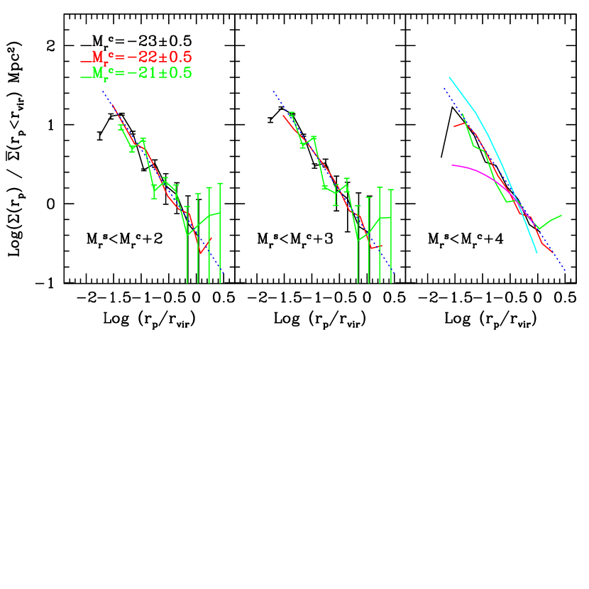
Figure 1.— The surface density of satellites as a function of the distance to the central galaxies. The surface density is scaled by the mean surface density within the virial radius, and the distance is scaled by the virial radius. From left to right: ${M_{r}}^{s}<{M_{r}}^{c}+2,{M_{r}}^{s}<{M_{r}}^{c}+3,{M_{r}}^{s}<{M_{r}}^{c}+4$. The blue dotted line is a fitting line with a slope of -1.05. The radial distributions for dark matter (cyan solid) and subhalos (purple solid) are also shown in the third panel. For clarity, error bars are plotted only for four subsamples, and those for other subsamples are comparable.

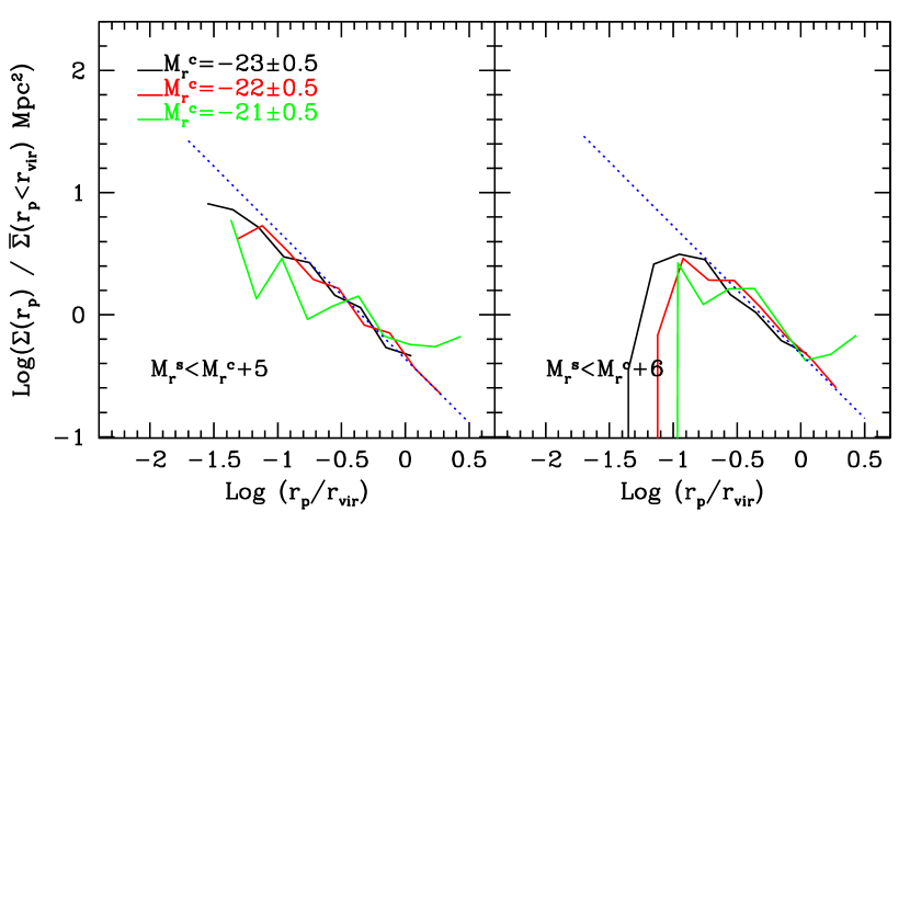
Figure 2.— Similar to Figure  1, but for satellites with ${M_{r}}^{s}<{M_{r}}^{c}+5$ and ${M_{r}}^{s}<{M_{r}}^{c}+6$.

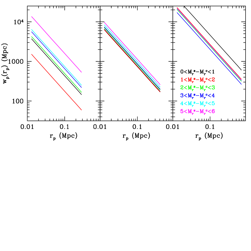
Figure 3.— Projected correlation functions for central galaxies with ${M_{r}}^{c}=-21,-22,-23$ from left to right, extending to virial radii.

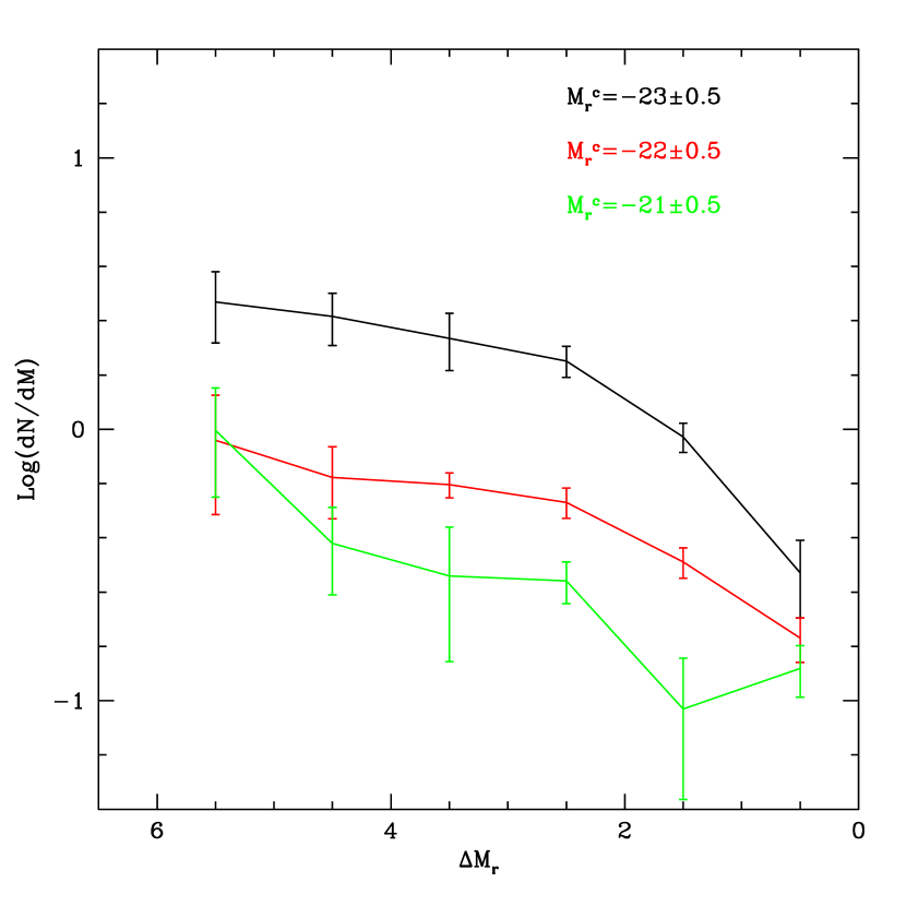
Figure 4.— Luminosity functions for central galaxies in the three magnitude bins within virial radii.

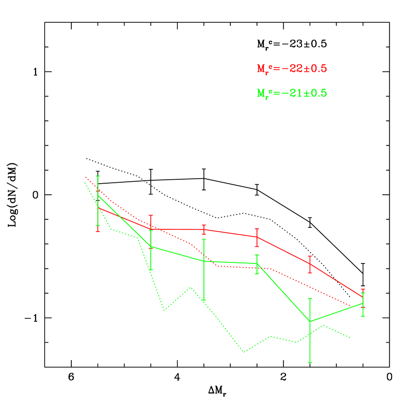
Figure 5.— Similar to Figure  4, but satellites are counted within projected distance 0.3 Mpc. In comparison, results of Guo et al. (2011) are shown with dotted lines.

Figure 6.— Luminosity functions for Milky Way-like central galaxies ($M_{\rm v}=-20.9\pm 0.5$) (black dotted) and Milky Way/M31-like central galaxies ($M_{\rm v}=-21.05\pm 0.5$) (black solid). The luminosity function of the Milky Way and M31 is plotted with red points (Koposov et al., 2008). The results of Guo et al. (2011) are shown with the blue solid line.

References

- Abazajian et al. (2009) Abazajian, K. N., Adelman-McCarthy, J. K., Agüeros, M. A., et al. 2009, ApJS, 182, 543
- Angulo et al. (2009) Angulo, R. E., Lacey, C. G., Baugh, C. M., & Frenk, C. S. 2009, MNRAS, 399, 983
- Arnouts et al. (1999) Arnouts, S., Cristiani, S., Moscardini, L., et al. 1999, MNRAS, 310, 540
- Blanton et al. (2003) Blanton, M. R., Hogg, D. W., Bahcall, N. A., et al. 2003, ApJ, 592, 819
- Blanton et al. (2005) Blanton, M. R., Schlegel, D. J., Strauss, M. A., et al. 2005, AJ, 129, 2562
- Boylan-Kolchin et al. (2010) Boylan-Kolchin, M., Springel, V., White, S. D. M., & Jenkins, A. 2010, MNRAS, 406, 896
- Busha et al. (2011) Busha, M. T., Wechsler, R. H., Behroozi, P. S., et al. 2011, ApJ, 743, 117
- Chen (2008) Chen, J. 2008, A&A, 484, 347
- Chen et al. (2006) Chen, J., Kravtsov, A. V., Prada, F., et al. 2006, ApJ, 647, 86
- Coupon et al. (2009) Coupon, J., Ilbert, O., Kilbinger, M., et al. 2009, A&A, 500, 981
- Davis & Peebles (1983) Davis, M., & Peebles, P. J. E. 1983, ApJ, 267, 465
- Dehnen et al. (2006) Dehnen, W., McLaughlin, D. E., & Sachania, J. 2006, MNRAS, 369, 1688
- Diemand et al. (2004) Diemand, J., Moore, B., & Stadel, J. 2004, MNRAS, 352, 535
- Gao et al. (2012) Gao, L., Navarro, J. F., Frenk, C. S., et al. 2012, arXiv:1201.1940
- Gao et al. (2004) Gao, L., White, S. D. M., Jenkins, A., Stoehr, F., & Springel, V. 2004, MNRAS, 355, 819
- Gao et al. (2008) Gao, L., Navarro, J. F., Cole, S., et al. 2008, MNRAS, 387, 536
- Ghigna et al. (2000) Ghigna, S., Moore, B., Governato, F., et al. 2000, ApJ, 544, 616
- Guo et al. (2010) Guo, Q., White, S., Li, C., & Boylan-Kolchin, M. 2010, MNRAS, 404, 1111
- Guo et al. (2011) Guo, Q., Cole, S., Eke, V., & Frenk, C. 2011, MNRAS, 417, 370
- Gwyn (2011) Gwyn, S. D. J. 2011, arXiv:1101.1084
- Han et al. (2011) Han, J., Jing, Y. P., Wang, H., & Wang, W. 2011, arXiv:1103.2099
- Ilbert et al. (2006) Ilbert, O., Arnouts, S., McCracken, H. J., et al. 2006, A&A, 457, 841
- Jiang et al. (2008) Jiang, C. Y., Jing, Y. P., Faltenbacher, A., Lin, W. P., & Li, C. 2008, ApJ, 675, 1095
- Jing & Suto (2000) Jing, Y. P., & Suto, Y. 2000, ApJ, 529, L69
- Klypin et al. (2001) Klypin, A., Kravtsov, A. V., Bullock, J. S., & Primack, J. R. 2001, ApJ, 554, 903
- Koposov et al. (2008) Koposov, S., Belokurov, V., Evans, N. W., et al. 2008, ApJ, 686, 279
- Koposov et al. (2009) Koposov, S. E., Yoo, J., Rix, H.-W., et al. 2009, ApJ, 696, 2179
- Kravtsov (2010) Kravtsov, A. 2010, Advances in Astronomy, 2010,
- Kravtsov et al. (2004) Kravtsov, A. V., Gnedin, O. Y., & Klypin, A. A. 2004, ApJ, 609, 482
- Lares et al. (2011) Lares, M., Lambas, D. G., & Domínguez, M. J. 2011, AJ, 142, 13
- Li et al. (2012) Li, C., Jing, Y. P., Mao, S., et al. 2012, arXiv:1206.3566
- Li et al. (2006) Li, C., Kauffmann, G., Jing, Y. P., et al. 2006, MNRAS, 368, 21
- Liu et al. (2011) Liu, L., Gerke, B. F., Wechsler, R. H., Behroozi, P. S., & Busha, M. T. 2011, ApJ, 733, 62
- Lovell et al. (2012) Lovell, M. R., Eke, V., Frenk, C. S., et al. 2012, MNRAS, 420, 2318
- Ludlow et al. (2009) Ludlow, A. D., Navarro, J. F., Springel, V., et al. 2009, ApJ, 692, 931
- Madau et al. (2008) Madau, P., Diemand, J., & Kuhlen, M. 2008, ApJ, 679, 1260
- Madore et al. (2004) Madore, B. F., Freedman, W. L., & Bothun, G. D. 2004, ApJ, 607, 810
- Mandelbaum et al. (2006) Mandelbaum, R., Seljak, U., Kauffmann, G., Hirata, C. M., & Brinkmann, J. 2006, MNRAS, 368, 715
- Merritt et al. (2006) Merritt, D., Graham, A. W., Moore, B., Diemand, J., & Terzić, B. 2006, AJ, 132, 2685
- Merritt et al. (2005) Merritt, D., Navarro, J. F., Ludlow, A., & Jenkins, A. 2005, ApJ, 624, L85
- More et al. (2011) More, S., van den Bosch, F. C., Cacciato, M., et al. 2011, MNRAS, 410, 210
- Moster et al. (2010) Moster, B. P., Somerville, R. S., Maulbetsch, C., et al. 2010, ApJ, 710, 903
- Navarro et al. (2004) Navarro, J. F., Hayashi, E., Power, C., et al. 2004, MNRAS, 349, 1039
- Navarro et al. (1997) Navarro, J. F., Frenk, C. S., & White, S. D. M. 1997, ApJ, 490, 493
- Nierenberg et al. (2012) Nierenberg, A. M., Auger, M. W., Treu, T., et al. 2012, arXiv:1202.2125
- Prada et al. (2006) Prada, F., Klypin, A. A., Simonneau, E., et al. 2006, ApJ, 645, 1001
- Regnault et al. (2009) Regnault, N., Conley, A., Guy, J., et al. 2009, A&A, 506, 999
- Robotham et al. (2012) Robotham, A. S. G., Baldry, I. K., Bland-Hawthorn, J., et al. 2012, MNRAS, 424, 1448
- Sakamoto et al. (2003) Sakamoto, T., Chiba, M., & Beers, T. C. 2003, A&A, 397, 899
- Sales & Lambas (2005) Sales, L., & Lambas, D. G. 2005, MNRAS, 356, 1045
- Smith et al. (2004) Smith, R. M., Martínez, V. J., & Graham, M. J. 2004, ApJ, 617, 1017
- Stanimirović et al. (2004) Stanimirović, S., Staveley-Smith, L., & Jones, P. A. 2004, ApJ, 604, 176
- Szapudi et al. (1992) Szapudi, I., Szalay, A. S., & Boschan, P. 1992, ApJ, 390, 350
- Tinker et al. (2005) Tinker, J. L., Weinberg, D. H., Zheng, Z., & Zehavi, I. 2005, ApJ, 631, 41
- van den Bergh (2000) van den Bergh, S. 2000, PASP, 112, 529
- van der Marel et al. (2002) van der Marel, R. P., Alves, D. R., Hardy, E., & Suntzeff, N. B. 2002, AJ, 124, 2639
- Wang et al. (2012) Wang, J., Frenk, C. S., Navarro, J. F., & Gao, L. 2012, arXiv:1203.4097
- Wang & Jing (2010) Wang, L., & Jing, Y. P. 2010, MNRAS, 402, 1796
- Wang et al. (2006) Wang, L., Li, C., Kauffmann, G., & De Lucia, G. 2006, MNRAS, 371, 537
- Wang et al. (2011) Wang, W., Jing, Y. P., Li, C., Okumura, T., & Han, J. 2011, ApJ, 734, 88
- Watson et al. (2010) Watson, D. F., Berlind, A. A., McBride, C. K., & Masjedi, M. 2010, ApJ, 709, 115
- Wilkinson & Evans (1999) Wilkinson, M. I., & Evans, N. W. 1999, MNRAS, 310, 645
- Xue et al. (2008) Xue, X. X., Rix, H. W., Zhao, G., et al. 2008, ApJ, 684, 1143
- Yang et al. (2003) Yang, X., Mo, H. J., & van den Bosch, F. C. 2003, MNRAS, 339, 1057
- Yang et al. (2007) Yang, X., Mo, H. J., van den Bosch, F. C., et al. 2007, ApJ, 671, 153
- York et al. (2000) York, D. G., Adelman, J., Anderson, J. E., Jr., et al. 2000, AJ, 120, 1579
- Zavala et al. (2009) Zavala, J., Jing, Y. P., Faltenbacher, A., et al. 2009, ApJ, 700, 1779
- Zehavi et al. (2005) Zehavi, I., Zheng, Z., Weinberg, D. H., et al. 2005, ApJ, 630, 1
- Zehavi et al. (2011) Zehavi, I., Zheng, Z., Weinberg, D. H., et al. 2011, ApJ, 736, 59
- Zheng et al. (2007) Zheng, Z., Coil, A. L., & Zehavi, I. 2007, ApJ, 667, 760