Distributed entanglement generation between continuous-mode Gaussian fields with measurement-feedback enhancement

Abstract

This paper studies a scheme of two spatially distant oscillator systems that are connected by Gaussian fields and examines distributed entanglement generation between two continuous-mode output Gaussian fields that are radiated by the oscillators. It is demonstrated that using measurement-feedback control while a non-local effective entangling operation is on can help to enhance the Einstein-Podolski-Rosen (EPR)-like entanglement between the output fields. The effect of propagation delays and losses in the fields interconnecting the two oscillators, and the effect of other losses in the system, are also considered. In particular, for a range of time delays the measurement feedback controller is able to maintain stability of the closed-loop system and the entanglement enhancement, but the achievable enhancement is only over a smaller bandwidth that is commensurate with the length of the time delays.

Abstract

This paper studies a scheme of two spatially distant oscillator systems that are connected by Gaussian fields and examines distributed entanglement generation between two continuous-mode output Gaussian fields that are radiated by the oscillators. It is demonstrated that using measurement-feedback control while a non-local effective entangling operation is on can help to enhance the Einstein-Podolski-Rosen (EPR)-like entanglement between the output fields. The effect of propagation delays and losses in the fields interconnecting the two oscillators, and the effect of other losses in the system, are also considered. In particular, for a range of time delays the measurement feedback controller is able to maintain stability of the closed-loop system and the entanglement enhancement, but the achievable enhancement is only over a smaller bandwidth that is commensurate with the length of the time delays.

I Introduction

Entanglement between quantum systems is considered to be an important resource to be exploited in many quantum-based technologies proposed in recent years. In particular, effective entanglement distribution in a quantum network is a problem that has attracted attention in the literature due to its importance in applications Cirac1997 ; Kimble2007 . However, entanglement is very fragile and the amount of entanglement can quickly be lost due to decoherence. One strategy to overcome this is to use several copies of quantum systems with a limited degree of entanglement and to process them to obtain a single copy that contains a higher degree of entanglement. This process is known as entanglement distillation Bennett1996 .

Researchers have considered entanglement distillation in both discrete and continuous variables. In the continuous variable case, a particular class of systems of interest are oscillator systems that are in a Gaussian state Ferraro2005 . If one has several copies of bipartite entangled pairs of Gaussian states then a no-go result of Eisert2002 states that it is not possible to distill further entanglement using only Gaussian local operation and classical communication (LOCC). Essentially, because the operations are LOCC there can be no entangling operations between any of the oscillators as they would necessarily have to be non-local. However, often in practice one considers dynamical quantum systems having an entangling interaction on during the evolution. The effectiveness of entanglement generation may be hampered by the decoherence taking place, possibly causing the entanglement to eventually vanish. Since there is a non-local entangling operation in effect, the no-go theorem does not hold, and this opens possibility to use Gaussian LOCC operations to protect entanglement during the system evolution. Thus, Mancini and Wiseman Mancini2007 considered the use of measurement feedback to improve entanglement between two cavity modes $a_{1}$ and $a_{2}$ coupled via a two mode squeezing Hamiltonian $H=i(\epsilon a_{1}^{*}a_{2}^{*}-\epsilon^{*}a_{1}a_{2})$; in this paper the notation ^∗ denotes the the adjoint of a Hilbert space operator or the conjugate transpose of a matrix of complex numbers or operators. At the same time, the two modes undergo decoherence, due to the cavity photons escaping through the transmissive cavity mirrors on which measurements can be made. They showed that there exists a Gaussian LOCC strategy realized by measurement-feedback that can help to improve the amount of entanglement between the two cavity modes compared to when no measurement and feedback is used. It was subsequently shown in Serafini2010 that the strategies proposed in Mancini2007 are optimal for that particular physical setup. Several other works in the literature have also considered using feedback for entanglement control, e.g., Carvalho2008 ; Yamamoto2008 ; WisemanBook ; Yan2011 .

The main contribution of this paper is developing a feedback-controlled scheme that uses distributed resources (parametric amplification at two spatially separate sites) to generate entanglement between two spatially separated continous-mode Gaussian fields. The system of interest is a quantum network consisting of two spatially separated open Gaussian oscillator systems. They are interconnected via travelling Gaussian quantum fields that act as common baths between the two oscillators and as a source of effective interaction between them. The scheme also exploits measurement-feedback control to enhance the entanglement. It is distinct from a measurement-feedback control based scheme on a linear quantum system studied in the earlier work Mancini2007 in several ways:

1. The scheme uses distributed resources. That is, entanglement is generated exploiting contributed resources at two spatially separated locations (say, at Alice and Bob’s). This use of spatially distributed resources for entanglement generation is a key feature of the proposed scheme. In contrast, Mancini2007 considers two oscillators interacting in a $\chi^{(2)}$ nonlinear crystal at a single location, and the entangling process occurs only at one site using only resources available at that site.

2. The paper is concerned with entanglement between two output fields, that consist of a continuum of modes, rather than entanglement between single mode internal oscillator modes as in Mancini2007 . Although the system in Mancini2007 does have output fields, they are only provided as observables to be measured and fedback rather than left freely as entangled resources. In contrast, the present work utilizes several output fields, some of which are for measurement and feedback while others remain free to be used as entangled resources. The rationale for considering entanglement in the output fields, rather than between internal oscillator modes, is that the output fields are more easily accessible to be exploited for various purposes. For instance, if multiple copies of the system are available then the multiple outputs of the various copies could, say, be passed onto some (at this stage hypothetical) entanglement distiller to produce another signal with improved EPR-like qualities.

3. Since generation of entanglement is via transmission channels linking the two spatially separated sites, there are inherent features of this scheme that need to be considered and which are not present in [6]. The first is the presence of losses along these transmission channels, and the second is the presence of time delays required for the interconnecting fields to propagate between the two sites.

In this work we show that a linear quadratic Gaussian (LQG) measurement-feedback controller WisemanBook ; Doherty1999 ; Belavkin2008 can enhance the entanglement between the output fields as compared to when there is no controller present. Moreover, this controller can provide an enhancement even in the presence of losses and delays in the overall system. That is, the controller displays robustness with respect to the presence of these imperfections. Simulation results are presented and discussed to compare the performance of the uncontrolled and controlled systems in the ideal case and in the presence of imperfections.

II Preliminaries

II.1 Linear quantum systems

In general, the dynamics of an open quantum system, which does not contain a scattering process, can be characterized by the system-environment coupling Hamiltonian

$$H_{\rm int}(t)=i\sum_{j=1}^{m}(L_{j}\xi_{j}(t)^{*}-L_{j}^{*}\xi_{j}(t)),$$ (1)

where $\xi_{j}(t)~{}(j=1,\ldots,m)$ is the field operator describing the $j$-th environment field and $L_{j}$ is the system operator corresponding to the $j$-th coupling GardinerBook . When the Markov limit is imposed on the environment, the field operators satisfy $[\xi_{i}(t),\xi_{j}(s)^{*}]=\delta(t-s)\delta_{ij}$.

A linear quantum system with $n$-bosonic modes $a_{j}(t)~{}(j=1,\ldots,n)$ satisfying $[a_{i},a_{j}^{*}]=\delta_{ij}$ appears when $L_{j}$ is linear and $H$ is quadratic in $a_{j}$ and $a_{j}^{*}$. In this case, the Heisenberg equation of $a_{j}(t)=U(t)^{*}a_{j}U(t)$ with unitary $U(t)={\rm exp}^{\longrightarrow}~{}(-i\int_{0}^{t}H_{\rm int}(s)ds)$ has the following form:

$$\dot{z}(t)=Az(t)+B\xi(t),$$ (2)

where we have defined

$$z=(a_{1}^{q},a_{1}^{p},\ldots,a_{n}^{q},a_{n}^{p})^{T},~{}~{}\xi=(\xi_{1}^{q},\xi_{1}^{p},\ldots,\xi_{m}^{q},\xi_{m}^{p})^{T},$$

with quadratures $a_{j}^{q}=a_{j}+a_{j}^{*}$, $a_{j}^{p}=(a_{j}-a_{j}^{*})/i$, $\xi_{j}^{q}=\xi_{j}+\xi_{j}^{*}$, and $\xi_{j}^{p}=(\xi_{j}-\xi_{j}^{*})/i$. The field operator also changes to $\xi_{out,j}(t)=U(t)^{*}\xi_{j}(t)U(t)$, and measuring this output field generates the classical signal

$$y(t)=Cz(t)+D\xi(t).$$ (3)

The system matrices $A,B,C$, and $D$ have specific structures to satisfy $[a_{i}(t),a_{j}(t)^{*}]=\delta_{ij}$ for all $t\geq 0$, and $[y(t),y(s)]=0$ for all $s,t\geq 0$.

II.2 Measurement-feedback LQG control

The field $\xi(t)$ can closely be approximated by a coherent light field generated from a laser device. Thus feedback control can be realized by replacing $\xi_{j}(t)$ by a modulated field $u_{j}(t)+\xi_{j}(t)$, where $u_{j}(t)$ is a function of $y(s)~{}(s\leq t)$.

In the LQG feedback control scheme, the control input $u(t)=(u_{1}^{q},u_{1}^{p},\ldots,u_{m}^{q},u_{m}^{p})$ is generated as an output of the following classical linear system with $y(t)$ as the input:

$$\dot{z}_{c}(t)=A_{c}z_{c}(t)+B_{c}y(t),~{}~{}~{}u(t)=C_{c}z_{c}(t).$$ (4)

$z_{c}(t)$ is a vector of real c-numbers representing the state of controller. $A_{c},~{}B_{c}$, and $C_{c}$ are real matrices to be designed. Combining Eqs. (2), (3), and (4), we have a closed-loop dynamics with variable $\tilde{z}=(z^{T},z_{c}^{T})^{T}$. For this system, we consider the following quadratic-type cost function:

$$J(u)=\mathop{\lim}_{T\rightarrow\infty}\frac{1}{T}{\mathbb{E}}\Big{[}\int_{0}^{T}\Big{\{}\tilde{z}(t)^{T}P\tilde{z}(t)+u(t)^{T}Qu(t)\Big{\}}dt\Big{]},$$ (5)

where $P\geq 0$ and $Q>0$ are weighting matrices that should be chosen appropriately. The expectation is defined as ${\mathbb{E}}(X)={\rm Tr}[X(\rho\otimes|{0}\rangle\langle{0}|)]$, where $\rho$ is the initial system Gaussian state and $|{0}\rangle$ is the field vacuum state. The optimal LQG feedback control input is given as a minimizer of the cost function (5); the minimization problem $\min J(u)$ can be efficiently solved using the Matlab Control System Toolbox to yield the optimal set of matrices $A_{c},B_{c}$, and $C_{c}$.

II.3 Frequency domain entanglement criteria for continuous-mode output fields

Let us here particularly focus on two output fields $\xi_{out,1}(t)$ and $\xi_{out,2}(t)$. These are continuous-mode fields, therefore we need to move to the frequency domain to evaluate their entanglement; for the quadratures $x_{j}=\xi_{out,j}+\xi_{out,j}^{*}$ and $y_{j}=(\xi_{out,j}-\xi_{out,j}^{*})/i$, define their Fourier transforms by $O_{j}(i\omega)=\int o_{j}(t)e^{-i\omega t}dt/\sqrt{2\pi}$ with $o=x,y$ and $O=X,Y$, respectively. Then the two output fields $\xi_{out,1}(t)$ and $\xi_{out,2}(t)$ are entangled for the mode at frequency $\omega$ if Vitali2006

$$V_{+}(i\omega)+V_{-}(i\omega)<4,$$ (6)

where $V_{+}(i\omega)$ and $V_{-}(i\omega)$ are defined by the identities

$$\langle(X_{1}(i\omega)+X_{2}(i\omega))^{*}(X_{1}(i\omega^{\prime})+X_{2}(i\omega^{\prime}))\rangle$$

$$~{}~{}=\langle(X_{1}(-i\omega)+X_{2}(-i\omega))(X_{1}(i\omega^{\prime})+X_{2}(i\omega^{\prime}))\rangle$$

$$~{}~{}=V_{+}(i\omega)\delta(\omega-\omega^{\prime}),$$

$$\langle(Y_{1}(i\omega)-Y_{2}(i\omega))^{*}(Y_{1}(i\omega^{\prime})-Y_{2}(i\omega^{\prime}))\rangle$$

$$~{}~{}=\langle(Y_{1}(-i\omega)-Y_{2}(-i\omega))(Y_{1}(i\omega^{\prime})-Y_{2}(i\omega^{\prime}))\rangle$$

$$~{}~{}=V_{-}(i\omega)\delta(\omega-\omega^{\prime}).$$

That is, $V_{+}(i\omega)$ and $V_{-}(i\omega)$ are power spectral densities of the fields. The inequality (6) is a well-known sufficient condition for entanglement in the frequency domain Ou1992 ; Vitali2006 . In the case of a two mode-squeezed state, the two power spectra are identical and, in an ideal limit, they converge to zero for all $\omega$, implying that the so-called Einstein-Podolski-Rosen (EPR) pair of fields is produced Ou1992 .

III The system model

III.1 Description

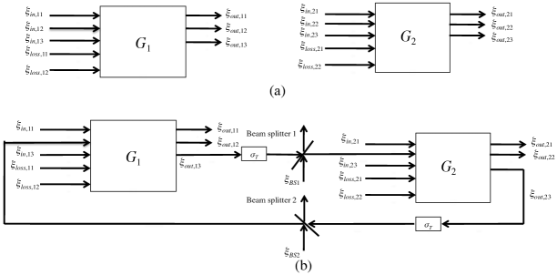
Figure 1: (a) Input and output fields of the open oscillators systems $G_{1}$ and $G_{2}$. In both systems, the output fields corresponding to the loss field $\xi_{loss,ij}$ cannot be essentially observed, hence they are not shown. (b) The connected open oscillator systems of $G_{1}$ and $G_{2}$. The traveling fields contain possible losses modeled by two beam splitters BS$1$ and BS$2$ with vacuum noises $\xi_{BS,1}$ and $\xi_{BS,2}$ entering into their unused ports, respectively. $\sigma_{T}$ denotes the operation bringing a time-delay $T$ on the traveling fields.

We consider the system shown in Fig. 1. The spatially separated open quantum systems $G_{1}$ and $G_{2}$ are connected by Gaussian quantum fields. The system $G_{j}$ consists of two oscillator modes $a_{j}$ and $b_{j}$ having the same oscillation frequency coupled to three independent quantum white noise fields $\xi_{in,j1}$, $\xi_{in,j2}$, and $\xi_{in,j3}$; they are continuous-mode and satisfy $[\xi_{in,jl}(t),\xi_{in,jl}(s)^{*}]=\delta(t-s)$. The oscillator modes satisfy the usual commutation relations $[a_{j},a_{k}^{*}]=\delta_{jk}$, $[b_{j},b^{*}_{k}]=\delta_{jk}$, $[a_{j},b_{k}]=0$, and $[a_{j},b_{k}^{*}]=0$ for $j,k=1,2$.

In system $G_{1}$, the modes $a_{1}$ and $b_{1}$ are coupled via the two-mode squeezing Hamiltonian $H_{1}=i\epsilon(a_{1}^{*}b^{*}_{1}-a_{1}b_{1})/2\sqrt{2}$ with $\epsilon$ constant. Moreover, $a_{1}$ is coupled to $\xi_{in,11}$ and $\xi_{in,12}$ via the coupling operators $L_{11}=\sqrt{\gamma}a_{1}$ and $L_{12}=i\sqrt{\kappa/2}a_{1}$, respectively, for some coupling constants $\gamma$ and $\kappa$. Also, $b_{1}$ is coupled to $\xi_{in,13}$ via $L_{13}=\sqrt{\kappa_{1}}b_{1}$ for coupling coefficient $\kappa_{1}$. We allow the possibility of losses in the two-mode squeezing process, which is modeled by the interaction of $a_{1}$ with the additional quantum noise field $\xi_{loss,11}$ via $L_{14}=\sqrt{\chi/2}a_{1}$ with $\chi$ a coupling constant. Similarly, $b_{1}$ interacts with $\xi_{loss,12}$ via $L_{15}=\sqrt{\chi/2}b_{1}$. The system $G_{2}$ has a similar structure. The modes $a_{2}$ and $b_{2}$ are coupled via the system Hamiltonian $H_{2}=-\epsilon(a_{2}^{*}b^{*}_{2}+a_{2}b_{2})/2\sqrt{2}$ with the same $\epsilon>0$. Also $a_{2}$ is coupled to $\xi_{in,21}$ and $\xi_{in,22}$ via $L_{21}=\sqrt{\gamma}a_{2}$ and $L_{22}=\sqrt{\kappa/2}a_{2}$, while $b_{2}$ is coupled to $\xi_{in,23}$ via $L_{23}=\sqrt{\kappa_{1}}b_{2}$. As in $G_{1}$, possible losses in the two-mode squeezing process in $H_{2}$ is modeled by coupling $a_{2}$ and $b_{2}$ to additional noise fields $\xi_{loss,21}$ and $\xi_{loss,22}$, respectively, via $L_{24}=\sqrt{\chi/2}a_{2}$ and $L_{25}=\sqrt{\chi/2}b_{2}$ with the same constant $\chi$ as before. The input fields $\xi_{in,j1}$, $\xi_{in,j3}$, $\xi_{loss,j1}$, and $\xi_{loss,j2}$ for $j=1,2$ are in the vacuum state.

We allow the possibility of photon losses in the two transmission channels connecting $G_{1}$ and $G_{2}$. The losses are modeled by inserting in the two transmission paths a beam splitter with transmissivity $\alpha$ and reflectivity $\beta$, with $\alpha^{2}+\beta^{2}=1$. Each beam splitter BS$j$ has two ports, one for the incoming signal $\xi_{out,j3}$ and an unused port for a noise field $\xi_{BS,j}$. Moreover, we also allow the possibility of time delays along these transmission channels that are represented in the figure by the $\sigma_{T}$ blocks, with $T$ a positive number indicating the transmission delay. The time delay block acts on a signal $\xi$ coming into the block as $(\sigma_{T}\xi)(t)=\xi(t-T)$. Thus the interconnecting fields satisfy $\alpha(\sigma_{T}\xi_{out,13})(t)+\beta\xi_{BS,1}(t)=\xi_{in,22}(t)$ and $\alpha(\sigma_{T}\xi_{out,23})(t)+\beta\xi_{BS,2}(t)=\xi_{in,12}(t)$. The dynamics of the whole network is then given as follows:

$$\dot{a}_{1}(t) =-(\frac{\gamma}{2}+\frac{\kappa}{4}+\frac{\chi}{4})a_{1}(t)+\frac{\epsilon}{2\sqrt{2}}b_{1}(t)^{*}-\sqrt{\gamma}\xi_{in,11}(t)$$

$$\quad+i\sqrt{\frac{\kappa}{2}}\Big{[}\alpha\Big{\{}\sqrt{\kappa_{1}}(\sigma_{T}b_{2})(t)+(\sigma_{T}\xi_{in,23})(t)\Big{\}}$$

$$\quad+\beta\xi_{BS,2}(t)\Big{]}-\sqrt{\frac{\chi}{2}}\xi_{loss,11}(t),$$

$$\dot{b}_{1}(t) =\frac{\epsilon}{2\sqrt{2}}a_{1}(t)^{*}-(\frac{\kappa_{1}}{2}+\frac{\chi}{4})b_{1}(t)-\sqrt{\kappa_{1}}\xi_{in,13}(t)$$

$$\quad-\sqrt{\frac{\chi}{2}}\xi_{loss,12}(t),$$

$$\dot{a}_{2}(t) =-(\frac{\gamma}{2}+\frac{\kappa}{4}+\frac{\chi}{4})a_{2}(t)+\frac{i\epsilon}{2\sqrt{2}}b_{2}(t)^{*}-\sqrt{\gamma}\xi_{in,21}(t)$$

$$\quad-\sqrt{\frac{\kappa}{2}}\Big{[}\alpha\Big{\{}\sqrt{\kappa_{1}}(\sigma_{T}b_{1})(t)+(\sigma_{T}\xi_{in,13})(t)\Big{\}}$$

$$\quad+\beta\xi_{BS,1}(t)\Big{]}-\sqrt{\frac{\chi}{2}}\xi_{loss,21}(t),$$

$$\dot{b}_{2}(t) =\frac{i\epsilon}{2\sqrt{2}}a_{2}(t)^{*}-(\frac{\kappa_{1}}{2}+\frac{\chi}{4})b_{2}(t)-\sqrt{\kappa_{1}}\xi_{in,23}(t)$$

$$\quad-\sqrt{\frac{\chi}{2}}\xi_{loss,22}(t),$$

with outputs

$$\xi_{out,11}(t) =\sqrt{\gamma}a_{1}(t)+\xi_{in,11}(t),$$

$$\xi_{out,12}(t) =i\sqrt{\frac{\kappa}{2}}a_{1}(t)+\alpha\sqrt{\kappa_{1}}(\sigma_{T}b_{2})(t)+\alpha(\sigma_{T}\xi_{in,23})(t)$$

$$\quad+\beta\xi_{BS,2}(t),$$

$$\xi_{out,21}(t) =\sqrt{\gamma}a_{2}(t)+\xi_{in,21}(t),$$

$$\xi_{out,22}(t) =\sqrt{\frac{\kappa}{2}}a_{2}(t)+\alpha\sqrt{\kappa_{1}}(\sigma_{T}b_{1})(t)+\alpha(\sigma_{T}\xi_{in,13})(t)$$

$$\quad+\beta\xi_{BS,1}(t).$$

The oscillator systems $G_{1}$ and $G_{2}$ could, in principle, be physically realized using optical cavities with $\chi^{(2)}$ nonlinear crystals, as depicted in Fig. 2. More precisely, the bow-tie type cavity $G_{1}$ contains two modes $a_{1}$ and $b_{1}$ that overlap and interact in a $\chi^{(2)}$ nonlinear crystal driven by a classical pump beam of effective amplitude $\epsilon/\sqrt{2}$. The modes $a_{1}$ and $b_{1}$ are frequency degenerate but orthogonally polarized. The mirrors composing the cavity are partially transmissive, depending on polarization of light fields; in particular, the mirrors $M_{11}$ and $M_{12}$ are partially transmissive for $a_{1}$ but perfectly reflective for $b_{1}$, while $M_{13}$ is partially transmissive for $b_{1}$ but perfectly reflective for $a_{1}$. The transmittance of $M_{11}$, $M_{12}$, and $M_{13}$ are $T_{11}=\gamma l/c$, $T_{12}=\kappa l/2c$, and $T_{13}=\kappa_{1}l/c$, respectively, with $l$ the optical path length of the cavity and $c$ the speed of light. In addition, the field $\xi_{in,12}$ entering through mirror $M_{12}$ and the output $\xi_{out,12}$ are both passed through a 180^o phase shifter. The system $G_{2}$ is similarly realized by a bow-tie type cavity. For a more detailed description, see e.g., Iida2012 .

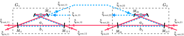
Figure 2: Candidate for a realization of the systems $G_{1}$ and $G_{2}$ in quantum optics. The modes $a_{1}$ and $b_{1}$ are frequency degenerate but orthogonally polarized. The mirrors composing the cavity $G_{1}$ are partially transmissive, depending on polarization of the light fields; the mirrors $M_{11}$ and $M_{12}$ are partially transmissive for $a_{1}$ but perfectly reflective for $b_{1}$, while $M_{13}$ is partially transmissive for $b_{1}$ but perfectly reflective for $a_{1}$. The cavity $G_{2}$ is also constructed in a similar way. For simplicity, other optical devices such as phase shifters are not shown.

The particular model described above is of interest because, in the large limit of the parameters that adiabatically eliminate $b_{1}$ and $b_{2}$ Nurdin2009 , and taking the limit of zero time delays along the transmission channels Gough2009a ; Gough2009b , the remaining modes $a_{1}$ and $a_{2}$ couple via the Hamiltonian $\hat{H}=-i\alpha\kappa(a_{1}^{*}a_{2}^{*}-a_{1}a_{2})$; this is a two-mode squeezing Hamiltonian which is the basis for generating entangled photon pairs in a nondegenerate optical parametric amplifier (NOPA) Ou1992 . In this sense, our system is a realistic approximation to the ideal system where two spatially separated systems effectively interact through this two-mode squeezing Hamiltonian.

III.2 Quadrature form and transfer function

We now specialize to the case where the transmission delay $T$ is negligible compared to the time scale of the dynamics of the systems $G_{1}$ and $G_{2}$. Then, in terms of quadratures, the coupled network Langevin equations with no transmission delays are:

$$\dot{a}^{q}_{1} =-(\frac{\gamma}{2}+\frac{\kappa}{4}+\frac{\chi}{4})a^{q}_{1}+\frac{\epsilon}{2\sqrt{2}}b^{q}_{1}-\alpha\sqrt{\frac{\kappa\kappa_{1}}{2}}b^{p}_{2}-\sqrt{\gamma}\xi^{q}_{in,11}$$

$$\quad-\alpha\sqrt{\frac{\kappa}{2}}\xi^{p}_{in,23}-\beta\sqrt{\frac{\kappa}{2}}\xi^{p}_{BS,2}-\sqrt{\frac{\chi}{2}}\xi^{q}_{loss,11},$$

$$\dot{a}^{p}_{1} =-(\frac{\gamma}{2}+\frac{\kappa}{4}+\frac{\chi}{4})a^{p}_{1}-\frac{\epsilon}{2\sqrt{2}}b^{p}_{1}+\alpha\sqrt{\frac{\kappa\kappa_{1}}{2}}b^{q}_{2}-\sqrt{\gamma}\xi^{p}_{in,11}$$

$$\quad+\alpha\sqrt{\frac{\kappa}{2}}\xi^{q}_{in,23}+\beta\sqrt{\frac{\kappa}{2}}\xi^{q}_{BS,2}-\sqrt{\frac{\chi}{2}}\xi^{p}_{loss,11},$$

$$\dot{b}^{q}_{1} =\frac{\epsilon}{2\sqrt{2}}a^{q}_{1}-(\frac{\kappa_{1}}{2}+\frac{\chi}{4})b^{q}_{1}-\sqrt{\kappa_{1}}\xi^{q}_{in,13}-\sqrt{\frac{\chi}{2}}\xi^{q}_{loss,12},$$

$$\dot{b}^{p}_{1} =-\frac{\epsilon}{2\sqrt{2}}a^{p}_{1}-(\frac{\kappa_{1}}{2}+\frac{\chi}{4})b^{p}_{1}-\sqrt{\kappa_{1}}\xi^{p}_{in,13}-\sqrt{\frac{\chi}{2}}\xi^{p}_{loss,12},$$

$$\dot{a}^{q}_{2} =-(\frac{\gamma}{2}+\frac{\kappa}{4}+\frac{\chi}{4})a^{q}_{2}+\frac{\epsilon}{2\sqrt{2}}b^{p}_{2}-\alpha\sqrt{\frac{\kappa\kappa_{1}}{2}}b^{q}_{1}-\sqrt{\gamma}\xi^{q}_{in,21}$$

$$\quad-\alpha\sqrt{\frac{\kappa}{2}}\xi^{q}_{in,13}+\beta\sqrt{\frac{\kappa}{2}}\xi^{q}_{BS,1}-\sqrt{\frac{\chi}{2}}\xi^{q}_{loss,21},$$

$$\dot{a}^{p}_{2} =-(\frac{\gamma}{2}+\frac{\kappa}{4}+\frac{\chi}{4})a^{p}_{2}+\frac{\epsilon}{2\sqrt{2}}b^{q}_{2}-\alpha\sqrt{\frac{\kappa\kappa_{1}}{2}}b^{p}_{1}-\sqrt{\gamma}\xi^{p}_{in,21}$$

$$\quad-\alpha\sqrt{\frac{\kappa}{2}}\xi^{p}_{in,13}-\beta\sqrt{\frac{\kappa}{2}}\xi^{p}_{BS,1}-\sqrt{\frac{\chi}{2}}\xi^{p}_{loss,21},$$

$$\dot{b}^{q}_{2} =\frac{\epsilon}{2\sqrt{2}}a^{p}_{2}-(\frac{\kappa_{1}}{2}+\frac{\chi}{4})b^{q}_{2}-\sqrt{\kappa_{1}}\xi^{q}_{in,23}-\sqrt{\frac{\chi}{2}}\xi^{q}_{loss,22},$$

$$\dot{b}^{p}_{2} =\frac{\epsilon}{2\sqrt{2}}a^{q}_{2}-(\frac{\kappa_{1}}{2}+\frac{\chi}{4})b^{p}_{2}-\sqrt{\kappa_{1}}\xi^{p}_{in,23}-\sqrt{\frac{\chi}{2}}\xi^{p}_{loss,22},$$

with outputs

$$\xi^{q}_{out,11} =\sqrt{\gamma}a^{q}_{1}+\xi^{q}_{in,11},~{}~{}~{}\xi^{p}_{out,11}=\sqrt{\gamma}a^{p}_{1}+\xi^{p}_{in,11},$$

$$\xi^{q}_{out,12} =-\sqrt{\frac{\kappa}{2}}a^{p}_{1}+\alpha\sqrt{\kappa_{1}}b_{2}^{q}+\alpha\xi^{q}_{in,23}+\beta\xi^{q}_{BS,2},$$

$$\xi^{p}_{out,12} =\sqrt{\frac{\kappa}{2}}a^{q}_{1}+\alpha\sqrt{\kappa_{1}}b_{2}^{p}+\alpha\xi^{p}_{in,23}+\beta\xi^{p}_{BS,2},$$

$$\xi^{q}_{out,21} =\sqrt{\gamma}a^{q}_{2}+\xi^{q}_{in,21},~{}~{}~{}\xi^{p}_{out,21}=\sqrt{\gamma}a^{p}_{2}+\xi^{p}_{in,21},$$

$$\xi^{q}_{out,22} =\sqrt{\frac{\kappa}{2}}a^{q}_{2}+\alpha\sqrt{\kappa_{1}}b^{q}_{1}+\alpha\xi^{q}_{in,13}+\beta\xi^{q}_{BS,1},$$

$$\xi^{p}_{out,22} =\sqrt{\frac{\kappa}{2}}a^{p}_{2}+\alpha\sqrt{\kappa_{1}}b^{p}_{1}+\alpha\xi^{p}_{in,13}+\beta\xi^{p}_{BS,1}.$$

Now, let us observe some properties of the above dynamical equations for the oscillator and field quadratures. In particular, from the above equations it can be verified that the equations are not fully coupled and in fact: (a) The set of equations for $a_{1}^{q},a_{2}^{q},b_{1}^{q}$, and $b_{2}^{p}$ form a closed set of equations driven by the commuting set of noises $\xi^{q}_{in,11}$, $\xi^{p}_{in,23}$, $\xi^{q}_{in,13}$, $\xi^{q}_{in,21}$, $\xi^{q}_{loss,11}$, $\xi^{q}_{loss,12}$, $\xi^{q}_{loss,21}$, $\xi^{p}_{loss,22}$, $\xi^{q}_{BS,1}$, and $\xi^{p}_{BS,2}$, and (b) the set of equations for $a_{1}^{p},a_{2}^{p},b_{1}^{p}$, and $b_{2}^{q}$ form another closed set of equations driven by the commuting set of noises $\xi^{p}_{in,11}$, $\xi^{q}_{in,23}$, $\xi^{p}_{in,13}$, $\xi^{p}_{in,21}$, $\xi^{p}_{loss,11}$, $\xi^{p}_{loss,12}$, $\xi^{p}_{loss,21}$, $\xi^{q}_{loss,22}$, $\xi^{p}_{BS,1}$, and $\xi^{q}_{BS,2}$. Although we are considering the case of no time delays, it may be easily inspected that the decoupling between the above sets of closed equations for certain quadratures and commuting noises also holds in the time delay case since the structure of the equations are precisely the same.

We can now consider the Fourier transforms of the observables above and the system transfer functions. Introduce the column vector of system operators

$$z_{1}(t) =(a_{1}^{q}(t),a_{2}^{q}(t),b_{1}^{q}(t),b_{2}^{p}(t),)^{T},$$

$$z_{2}(t) =(a_{1}^{p}(t),a_{2}^{p}(t),b_{1}^{p}(t),b_{2}^{q}(t))^{T},$$

$$z(t) =(z_{1}(t)^{T},z_{2}(t)^{T})^{T},$$

and

$$\xi_{1} =(\xi^{q}_{in,11},\xi^{p}_{in,23},\xi^{q}_{in,13},\xi^{q}_{in,21},$$

$$\quad\xi^{q}_{loss,11},\xi^{q}_{loss,12},\xi^{q}_{loss,21},\xi^{p}_{loss,22},\xi^{q}_{BS,1},\xi^{p}_{BS,2})^{T},$$

$$\xi_{2} =(\xi^{p}_{in,11},\xi^{q}_{in,23},\xi^{p}_{in,13},\xi^{p}_{in,21},$$

$$\quad\xi^{p}_{loss,11},\xi^{p}_{loss,12},\xi^{p}_{loss,21},\xi^{q}_{loss,22},\xi^{p}_{BS,1},\xi^{q}_{BS,2})^{T},$$

$$\xi =(\xi_{1}(t)^{T},\xi_{2}(t)^{T})^{T}.$$

By the decoupling structure already noted above, we have

$$\dot{z}_{j}(t)=A_{j}z_{j}(t)+B_{j}\xi_{j}(t),~{}~{}~{}(j=1,2),$$

$$\xi^{q}_{out,11}(t)+\xi^{q}_{out,21}(t)=C_{1}z_{1}(t)+D_{1}\xi_{1}(t),$$

$$\xi^{p}_{out,11}(t)-\xi^{p}_{out,21}(t)=C_{2}z_{2}(t)+D_{2}\xi_{2}(t),$$

where $A_{1},A_{2},B_{1}$, and $B_{2}$ are real matrices of suitable dimensions whose entries can be readily determined from the equations for $a_{j}^{q},a_{j}^{p},b_{j}^{q}$, and $b_{j}^{p}$, and the row vectors $C_{1}$, $C_{2}$, $D_{1}$, and $D_{2}$ are given by:

$$C_{1} =(1,~{}1,~{}0_{1\times 2}),~{}~{}~{}C_{2}=(1,~{}-1,~{}0_{1\times 2}),$$

$$D_{1} =(1,~{}0_{1\times 3},~{}1,~{}0_{1\times 6}),~{}~{}~{}D_{2}=(1,~{}0_{1\times 3},~{}-1,~{}0_{1\times 6}).$$

Let $x_{j}(t)=\xi^{q}_{out,j1}(t)$ and $y_{j}(t)=\xi^{p}_{out,j1}(t)$ and let $X_{j}$, $Y_{j}$, and $\Xi_{j}$ denote the Fourier transforms of $x_{j}$, $y_{j}$, and $\xi_{j}$, respectively (see Section II.3). Then

$$X_{1}(i\omega)+X_{2}(i\omega)=H_{1}(i\omega)\Xi_{1}(i\omega),$$

$$Y_{1}(i\omega)-Y_{2}(i\omega)=H_{2}(i\omega)\Xi_{2}(i\omega),$$

with $H_{j}(i\omega)=C_{j}(i\omega I-A_{j})^{-1}B_{j}+D_{j}$ ($j=1,2$). Using the fact that $\langle(\Xi_{j}(i\omega)^{*})^{T}\Xi_{j}(i\omega^{\prime})^{T}\rangle=\langle\Xi_{j}(-i\omega)\Xi_{j}(i\omega^{\prime})^{T}\rangle=I_{10\times 10}\delta(\omega-\omega^{\prime})$, we find that $\langle(X_{1}(i\omega)+X_{2}(i\omega))^{*}(X_{1}(i\omega^{\prime})+X_{2}(i\omega^{\prime}))\rangle={\rm Tr}[H_{1}(i\omega)^{*}H_{1}(i\omega)]\delta(\omega-\omega^{\prime})$ and $\langle(Y_{1}(i\omega)-Y_{2}(i\omega))^{*}(Y_{1}(i\omega^{\prime})-Y_{2}(i\omega^{\prime}))\rangle={\rm Tr}[H_{2}(i\omega)^{*}H_{2}(i\omega)]\delta(\omega-\omega^{\prime})$. Thus, for the uncontrolled network we conclude that

$$V_{+}(i\omega)={\rm Tr}[H_{1}(i\omega)^{*}H_{1}(i\omega)],$$

$$V_{-}(i\omega)={\rm Tr}[H_{2}(i\omega)^{*}H_{2}(i\omega)].$$

IV LQG feedback control of the system

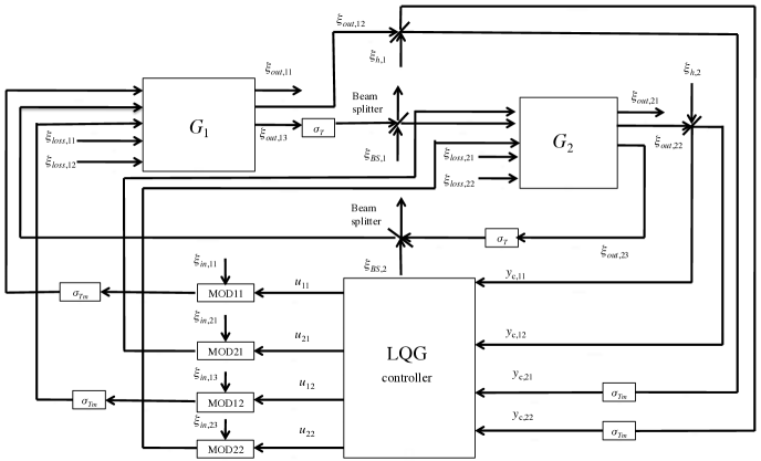
Figure 3: The controlled quantum network. The LQG controller is located on the site of $G_{2}$; hence the time delays of communication between the controller and the system $G_{2}$ is negligible, while we assume that the control signals $u_{11}$ and $u_{12}$ propagate from the controller to $G_{1}$ with time delays $T_{m}$. The operation bringing this time-delay is denoted by $\sigma_{T_{m}}$.

The control scheme is shown in Fig. 3. The input to the controller will be the signals $y_{c,11}$, $y_{c,12}$, $y_{c,21}$, and $y_{c,22}$ that are obtained by performing dual homodyne detection on the output fields $\xi_{out,12}$ and $\xi_{out,22}$, respectively. Two dual homodyne detectors, labeled 1 and 2, are required, and each consists of a 50:50 beam splitter, where at the unused beam splitter port a vacuum noise source $\xi_{h,j},(j=1,2)$ comes in. At the output of one beam splitter, the position quadrature of the field is measured while at the other output the momentum quadrature is measured. For the $j$-th dual homodyne detector, the outputs $y_{c,j1}$ and $y_{c,j2}$ are given by:

$$y_{c,11}(t) =\frac{\sqrt{\kappa}}{2}a^{q}_{2}(t)+\alpha\sqrt{\frac{\kappa_{1}}{2}}b^{q}_{1}(t)+\frac{\alpha}{\sqrt{2}}\xi^{q}_{in,13}(t)$$

$$\quad+\frac{\beta}{\sqrt{2}}\xi^{q}_{BS,1}(t)+\frac{1}{\sqrt{2}}\xi^{q}_{h,2}(t),$$ (7)

$$y_{c,12}(t) =-\frac{\sqrt{\kappa}}{2}a^{p}_{2}(t)-\alpha\sqrt{\frac{\kappa_{1}}{2}}b^{p}_{1}(t)-\frac{\alpha}{\sqrt{2}}\xi^{p}_{in,13}(t)$$

$$\quad-\frac{\beta}{\sqrt{2}}\xi^{p}_{BS,1}(t)+\frac{1}{\sqrt{2}}\xi^{p}_{h,2}(t),$$ (8)

$$y_{c,21}(t) =-\frac{\sqrt{\kappa}}{2}(\sigma_{T}a^{p}_{1})(t)+\alpha\sqrt{\frac{\kappa_{1}}{2}}(\sigma_{T}b^{q}_{2})(t)$$

$$\quad+\frac{\alpha}{\sqrt{2}}(\sigma_{T}\xi^{q}_{in,23})(t)+\frac{\beta}{\sqrt{2}}(\sigma_{T}\xi^{q}_{BS,2})(t)$$

$$\quad+\frac{1}{\sqrt{2}}(\sigma_{T}\xi^{q}_{h,1})(t),$$ (9)

$$y_{c,22}(t) =-\frac{\sqrt{\kappa}}{2}(\sigma_{T}a^{q}_{1})(t)-\alpha\sqrt{\frac{\kappa_{1}}{2}}(\sigma_{T}b^{p}_{2})(t)$$

$$\quad-\frac{\alpha}{\sqrt{2}}(\sigma_{T}\xi^{p}_{in,23})(t)-\frac{\beta}{\sqrt{2}}(\sigma_{T}\xi^{p}_{BS,2})(t)$$

$$\quad+\frac{1}{\sqrt{2}}(\sigma_{T}\xi^{p}_{h,1})(t),$$ (10)

The controller produces 8 control signals $u^{q}_{j1}(t)$, $u^{p}_{j1}(t)$, $u^{q}_{j2}(t)$, and $u^{p}_{j2}(t)$ for $j=1,2$ which drive the quantum system via modulators. The control signals $u^{q}_{jl}$ and $u^{p}_{jl}$ form the real and imaginary component of the complex classical signal $u_{jl}=u_{jl}^{q}+iu^{p}_{jl}$ that will drive the modulator labeled MOD$jl$ for $j,l=1,2$. The output of the modulator MOD$jl$ then drives the system $G_{j}$, see Fig. 3. The position and momentum quadratures of the output field of MOD$j1$ are $u^{q}_{j1}(t)+\xi^{q}_{in,j1}$ and $u^{p}_{j1}(t)+\xi^{p}_{in,j1}$, respectively, while the position and momentum quadratures of the output field MOD$j2$ are $u^{q}_{j2}(t)+\xi^{q}_{in,j3}$ and $u^{p}_{j2}(t)+\xi^{p}_{in,j3}$, respectively. Let $y_{c}(t)=(y_{c,11}(t),y_{c,12}(t),y_{c,21}(t),y_{c,22}(t))^{T}$ and

$$u_{c}=(u^{q}_{11},u^{p}_{11},u^{q}_{21},u^{p}_{21},u^{q}_{12},u^{p}_{12},u^{q}_{22},u^{p}_{22})^{T}.$$

The LQG controller has an internal 8-th order state $z_{c}(t)$ that obeys the following classical Langevin equation:

$$\dot{z}_{c}(t)=A_{c}z_{c}(t)+B_{c}y_{c}(t),~{}~{}~{}u_{c}(t)=C_{c}z_{c}(t),$$ (11)

where $A_{c}$, $B_{c}$, $C_{c}$ are real matrices of the appropriate dimensions. Here, the order of $z_{c}(t)$ is 8, since the degree of the system to be controlled is 8, corresponding to the oscillator quadratures $a_{j}^{q}$, $a_{j}^{p}$, $b_{j}^{q}$, and $b_{j}^{p}$ for $j=1,2$.

We assume that the controller is located on the site of $G_{2}$ so that the delays in transmitting the control signals $u_{21}$ and $u_{22}$ from the controller to the system $G_{2}$ are negligible. However, we allow the possibility of delays in transmitting the control signals $u_{11}$ and $u_{12}$ from the controller to $G_{1}$; here we assume those time delays take the same quantities and let us denote them by $T_{m}$. Then, the dynamical equation for the closed loop system can be obtained simply by making the substitutions of Eqs. (7)-(10) into Eq. (11) and the substitutions

$$\sigma_{T_{m}}(u_{11}+\xi_{in,11})\rightarrow\xi_{in,11},~{}~{}\sigma_{T_{m}}(u_{12}+\xi_{in,13})\rightarrow\xi_{in,13},$$

$$u_{21}+\xi_{in,21}\rightarrow\xi_{in,21},~{}~{}u_{22}+\xi_{in,23}\rightarrow\xi_{in,23}$$

into the dynamical equations of the system. Now define

$$\tilde{z}=(z^{T},z_{c}^{T})^{T},~{}~{}~{}\tilde{\xi}=(\xi^{T},\xi^{q}_{h,1},\xi^{p}_{h,1},\xi^{q}_{h,2},\xi^{p}_{h,2})^{T}.$$

The closed-loop system without time delays is then given by

$$\dot{\tilde{z}}(t)=\tilde{A}\tilde{z}(t)+\tilde{B}\tilde{\xi}(t),$$

where $\tilde{A}$ and $\tilde{B}$ are real matrices of the form:

$$\tilde{A}=\left(\begin{array}[]{ccc}A_{1}&0&A_{13}\\ 0&A_{2}&A_{23}\\ A_{31}&A_{32}&A_{33}\end{array}\right),~{}~{}\tilde{B}=\left(\begin{array}[]{ccc}B_{1}&0&0\\ 0&B_{2}&0\\ B_{31}&B_{32}&B_{33}\\ \end{array}\right).$$

Here, $A_{1}$, $A_{2}$, $B_{1}$, and $B_{2}$ are as defined previously in Sec. III.2, and $A_{jl}$ and $B_{jl}$ are matrices that are determined by the resulting closed-loop system. The equations for $\xi^{q}_{out,11}+\xi^{q}_{out,21}$ and $\xi^{p}_{out,11}-\xi^{p}_{out,21}$ are now of the form:

$$\xi^{q}_{out,11}(t)+\xi^{q}_{out,21}(t) =(C_{1},~{}0_{1\times 4},~{}C_{12})z(t)+\tilde{D}_{1}\tilde{\xi}(t),$$

$$\xi^{p}_{out,11}(t)-\xi^{p}_{out,21}(t) =(0_{1\times 4},~{}C_{2},~{}C_{22})z(t)+\tilde{D}_{2}\tilde{\xi}(t),$$

with $C_{1}$ and $C_{2}$ also as given in Sec. III.2, and $\tilde{D}_{1}=(D_{1},~{}0_{1\times 14})$ and $\tilde{D}_{2}=(0_{1\times 10},~{}D_{2},~{}0_{1\times 4})$. Note that there are contributions from the classical controller state $z_{c}(t)$ of the controller in these quadratures. However, since we are interested in the entanglement between the output fields, we can omit these contributions, since they, being classical, have no bearing on the degree of entanglement. Thus, in the case of a measurement-feedback controller in the loop it suffices to consider the modified outputs

$$\tilde{\xi}^{q}_{out,11}(t)+\tilde{\xi}^{q}_{out,21}(t) =(C_{1},~{}0_{1\times 12})z(t)+\tilde{D}_{1}\tilde{\xi}(t),$$

$$\tilde{\xi}^{p}_{out,11}(t)-\tilde{\xi}^{p}_{out,21}(t) =(0_{1\times 4},~{}C_{2},~{}0_{1\times 8})z(t)+\tilde{D}_{2}\tilde{\xi}(t).$$

Define $x_{1}(t)=\tilde{\xi}^{q}_{out,11}(t)$, $x_{2}(t)=\tilde{\xi}^{q}_{out,21}(t)$, $y_{1}(t)=\tilde{\xi}^{p}_{out,11}(t)$, and $y_{2}(t)=\tilde{\xi}^{p}_{out,21}(t)$ and let $X_{1}(i\omega)$, $X_{2}(i\omega)$, $Y_{1}(i\omega)$, and $Y_{2}(i\omega)$ be their Fourier transforms, respectively. Also, let $\tilde{\Xi}(i\omega)$ denote the Fourier transform of $\tilde{\xi}(t)$. Then, the transfer function $\tilde{H}_{1}(i\omega)$ from $\tilde{\Xi}(i\omega)$ to $X_{1}(i\omega)+X_{2}(i\omega)$ and $\tilde{H}_{2}(i\omega)$ from $\tilde{\Xi}(i\omega)$ to $Y_{1}(i\omega)-Y_{2}(i\omega)$ are given by

$$\tilde{H}_{1}(i\omega) =(C_{1},~{}0_{1\times 12})(i\omega I-\tilde{A})^{-1}\tilde{B}+\tilde{D}_{1},$$

$$\tilde{H}_{2}(i\omega) =(0_{1\times 4},~{}C_{2},~{}0_{1\times 8})(i\omega I-\tilde{A})^{-1}\tilde{B}+\tilde{D}_{2}.$$

Then, noting that $\langle(\tilde{\Xi}(i\omega)^{*})^{T}\tilde{\Xi}(i\omega^{\prime})^{T}\rangle=\langle\tilde{\Xi}(-i\omega)\tilde{\Xi}(i\omega^{\prime})^{T}\rangle=(I_{24\times 24}+iZ)\delta(\omega-\omega^{\prime})$, we obtain the expressions:

$$\langle(X_{1}(i\omega)+X_{2}(i\omega))^{*}(X_{1}(i\omega^{\prime})+X_{2}(i\omega^{\prime}))\rangle$$

$$\quad={\rm Tr}\bigl{[}(\tilde{H}_{1}(i\omega)^{*}\tilde{H}_{1}(i\omega))^{T}(I_{24\times 24}+iZ)\bigr{]}\delta(\omega-\omega^{\prime}),$$

$$\quad={\rm Tr}\big{[}\tilde{H}_{1}(i\omega)^{*}\tilde{H}_{1}(i\omega)\big{]}\delta(\omega-\omega^{\prime}),$$

$$\langle(Y_{1}(i\omega)-Y_{2}(i\omega))^{*}(Y_{1}(i\omega^{\prime})-Y_{2}(i\omega^{\prime}))\rangle$$

$$\quad={\rm Tr}\bigl{[}(\tilde{H}_{2}(i\omega)^{*}\tilde{H}_{2}(i\omega))^{T}(I_{24\times 24}+iZ)\bigr{]}\delta(\omega-\omega^{\prime}),$$

$$\quad={\rm Tr}\big{[}\tilde{H}_{2}(i\omega)^{*}\tilde{H}_{2}(i\omega)\big{]}\delta(\omega-\omega^{\prime}).$$

Here, $Z$ is a real invertible $24\times 24$ skew-symmetric matrix given by $Z=\frac{1}{2i}\langle\tilde{\Xi}(-i\omega)\tilde{\Xi}(i\omega)^{T}-(\tilde{\Xi}(-i\omega)\tilde{\Xi}(i\omega)^{T})^{T}\rangle$. Therefore, we conclude that the expressions for $V_{+}(i\omega)$ and $V_{-}(i\omega)$ when there is an LQG controller in the loop are

$$V_{+}(i\omega) ={\rm Tr}\big{[}\tilde{H}_{1}(i\omega)^{*}\tilde{H}_{1}(i\omega)\big{]},$$

$$V_{-}(i\omega) ={\rm Tr}\big{[}\tilde{H}_{2}(i\omega)^{*}\tilde{H}_{2}(i\omega)\big{]}.$$

V Entanglement between continuous-mode Gaussian output fields: The ideal case

We here consider the entanglement generated between $\xi_{out,11}(t)$ and $\xi_{out,21}(t)$, with and without an LQG feedback controller, in the idealized situation where there are no losses in the two mode squeezing processes (i.e., $\chi=0$) and there are also no losses in the transmission channels between $G_{1}$ and $G_{2}$ (i.e., $\alpha=1$). First, we assume that the transmission delays along the transmission channels are negligible. Then we will consider how the control performance and the closed-loop stability are affected by non-negligible time delays.

V.1 Negligible transmission delays

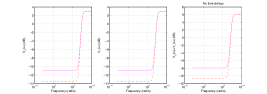
Figure 4: Plots of $V_{+}(i\omega)$ (left), $V_{-}(i\omega)$ (middle), and $V_{-}(i\omega)+V_{+}(i\omega)$ (right) in dB against the frequency in rad/s, without an LQG controller (solid line) and with an LQG controller (dashed line) designed to minimize the cost function (14). The same lines are used as legends in subsequent figures as well.

Throughout we will consider the case where $\kappa=1.8\times 10^{7}$ Hz, $\gamma=1.5\times\kappa=2.7\times 10^{7}$ Hz, $\kappa_{1}=10\times\kappa=1.8\times 10^{8}$ Hz, and $\epsilon/\sqrt{2}=\sqrt{\kappa\kappa_{1}/2}=4.0249\times 10^{7}$ Hz. In the case of the optical system shown in Fig. 2, these parameter values are realized using the mirrors with transmittance $T_{11}=T_{21}=0.045$, $T_{12}=T_{22}=0.015$, and $T_{13}=T_{23}=0.3$, where the optical path lengths of each cavities are both set to $l=0.5$ m. In this section we also set $\alpha=1$ and $T=T_{m}=0$. To design an 8th-order LQG controller, let us set the cost function (5) in the following form:

$$J(u_{c}) =\mathop{\lim}_{T\rightarrow\infty}\frac{1}{T}{\mathbb{E}}\Big{[}\int_{0}^{T}\Big{\{}\varrho\big{(}\left[\begin{array}[]{cc}C_{1}&C_{2}\end{array}\right]z(t)\big{)}^{2}$$ (13)

$$\qquad+u_{c}(t)^{T}u_{c}(t)\Big{\}}dt\Big{]}.$$ (14)

The weighting constant $\varrho$ is taken to be $\varrho=1\times 10^{7}$. With the use of the Matlab Control System Toolbox, we obtain the optimal LQG controller, and we show the frequency domain power spectra plots $V_{+}(i\omega)$, $V_{-}(i\omega)$, and $V_{+}(i\omega)+V_{-}(i\omega)$ in Fig. 4 in dB scale (here $A\geq 0$ in linear scale is $10\log_{10}A$ in dB scale). These figures indicate that all three power spectra are lower when the LQG controller is present as compared to when there is no controller. Here the controller can provide an additional attenuation to all three spectra by slightly more than 2.6 dB up to frequency of about $10^{6}$ rad/s. Moreover, by the entanglement criterion (6), we see that entanglement is achieved for modes with frequency up to slightly above $10^{7}$ rad/s but less than $10^{8}$ rad/s (note that entanglement is achieved at a mode of frequency $\omega$ whenever $V_{+}(i\omega)+V_{-}(i\omega)<10\log_{10}(4)\,\hbox{dB}=6.0206\,\hbox{dB}$). Note that this is achieved despite the controller being designed to minimize the cost function (14) rather than minimizing any of the three power spectra directly, indicating the utility of the cost function (14) for feedback control of output entanglement.

V.2 Non-negligible transmission delays

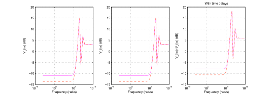
Figure 5: Plots of $V_{+}(i\omega)$ (left), $V_{-}(i\omega)$ (middle), and $V_{-}(i\omega)+V_{+}(i\omega)$ (right) in dB against the frequency in rad/s when there are time delays present ($T=1\times 10^{-6}$ s and $T_{m}=2\times 10^{-6}$ s).

Since the dynamics of $z(t)$ and $z_{c}(t)$ preserves the Gaussian nature of the state, we can study an equivalent linear classical delayed differential Gaussian system with finite time delays (in the sense that the mean and (symmetrized) covariance matrix of the quantum system and its classical equivalent evolve in an identical manner). See, e.g., the text Michiels2007 for a treatment of classical linear systems with time delays. Such linear differential systems with delays can be handled with the Matlab Control System Toolbox’s ‘delayss’ object. We consider the case where $T=10^{-6}$ s and $T_{m}=2\times 10^{-6}$ s, which is about an order of magnitude longer than the time scale of the system dynamics. Using the controller that had been designed in Sec. V.1, we obtain plots of $V_{+}(i\omega)$, $V_{-}(i\omega)$, and $V_{+}(i\omega)+V_{-}(i\omega)$ as shown in Fig. 5. They indicate that despite the time delays there is still a significant reduction of about 2.6 dB in all three spectra for frequencies up to about $10^{4}$ rad/s and 1 dB for frequencies between $10^{4}$ and $10^{5}$ rad/s. Slightly above $10^{5}$ rad/s, there is no more reduction and in fact one can see a marked increase in the magnitude of each spectra at certain frequencies above $10^{5}$ rad/s. This suggests that the feedback controller is still effective for enhancing the entanglement between the output fields even in the presence of time delays, but the bandwidth at which enhancement is achieved is reduced. However, additional care has to be taken before we can be conclusive about this claim. As we have seen, there are frequency ranges in which all three spectra experience a large increase, which could be indicative of instability (instability here is in the sense that the symmetrized covariance matrix of the system diverges as $t\rightarrow\infty$). Linear delay differential systems can be described by abstract infinite-dimensional differential equations Michiels2007 , and numerical algorithms are available to examine the stability of these systems. Here we use the freely available DDE-BIFTOOL toolbox Engelborghs2001 ; Engelborghs2002 , a Matlab toolbox to determine the stability of a delay differential system, and find that the system under consideration is indeed stable, the right hand most root of the characteristic equation of the system has a negative real part .

Note that the log-log nature of the plots and the number of points used to produce Fig. 5 (as well as Fig. 10) in Matlab give the impression of non-smooth functions, but in fact this is not the case. Since the analysis shows that the closed-loop system is stable, the closed-loop transfer function has no poles on the right half plane and all poles are bounded away from the imaginary axis and thus the functions $V_{\pm}(i\omega)$ depicted in the plots are theoretically guaranteed to be smooth functions of $\omega$ (i.e., they infinitely differentiable functions of $\omega$). However, the plots indicate that when there are time delays these functions fluctuate faster at some high frequencies. The fluctuations in the figures are prominent since the time delays have been taken to be comparable to the time scale of the node dynamics. If the delays are gradually decreased to zero then the high frequency fluctuations gradually smooths out.

VI Effect of amplification losses and transmission losses

Here we consider the more realistic case where there are losses in the two-mode squeezing process and along the transmission lines connecting $G_{1}$ and $G_{2}$. We will design our LQG controller based on the assumption that we do not how much these losses appear in the system, effectively. Thus we set the controller to be identical to the one we had previously designed under the assumption $\chi=0$ and $\alpha=1$.

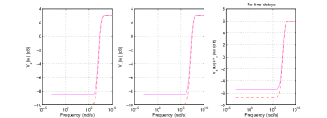
Figure 6: Performance of the system when the amplification loss is $\chi=1.3975\times 10^{6}$ Hz, no transmission losses, and there are no delays.

We consider first the case where the amplification loss coefficient is $\chi=1.3975\times 10^{6}$ Hz and there are no transmission losses ($\alpha=1$). The results are shown in Fig. 6. It can be seen that in the frequency region where the controller can reduce the power spectra, the reduction is smaller than if there were no amplification losses (about 1.4 dB reduction compared to about 2.6 dB reduction in the latter). For the same amplification loss coefficient, the cases with transmission losses of 3% ($\alpha=0.97)$ and 5% ($\alpha=0.95$) are shown in Figs. 7 and 8, respectively. Comparing Fig. 4 and Fig. 6, we see that, as can be expected, the presence of amplification loss has an adverse effect on the EPR-like entanglement that can be observed at the output; that is, all the power spectra are amplified at frequencies up to $10^{7}$ rad/s. Figs. 6-8 then show that the presence of increasing transmission losses leads to a corresponding increase in the power spectra across the same frequencies and thus a worsening of the quality of the EPR-like entanglement in the output fields. However, in all of these cases, it is clear that the presence of a controller leads to an improvement in the entanglement. Moreover, this is despite the fact that the controller was designed under the assumption that $\chi=0$ and $\alpha=1$. That is, the controller exhibits a level of robustness in its ability to improve the system performance.

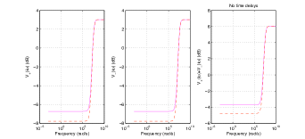
Figure 7: Performance of the system when the amplification loss coefficient is $\chi=1.3975\times 10^{6}$ Hz, transmission losses of 3%, and there are no delays.

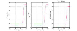
Figure 8: Performance of the system when the amplification loss coefficient is $\chi=1.3975\times 10^{6}$ Hz, transmission losses of 5%, and there are no delays.

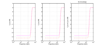
Figure 9: Performance of the system when the amplification loss coefficient is $\chi=5.5902\times 10^{6}$ Hz, transmission losses of 5%, and there are no time delays.

Finally, Fig. 9 shows the case where $\chi=5.5902\times 10^{6}$ Hz, which is a substantial percentage of amplification loss compared to pump intensity, and the transmission loss is $5\%$. Here, again, the time delays are assumed to be zero. The figure indicates that the LQG controller still manages to improve entanglement although the power spectra are, as can be expected, noticeably higher than those in Figs. 4-8. Finally, for the same values of $\chi$ and $\alpha$, the effect of the presence of the time delays $T=10^{-6}$ s and $T_{m}=2\times 10^{-6}$ s is shown in Fig. 10. As we had seen in Fig. 5, the delays reduce the frequency range in which a reduction in the power spectra by the controller can be observed. In particular, in the frequency range up to about $10^{5}$ rad/s, where the reduction is observed, the amount of reduction is roughly the same as what can be achieved without the delays. Also, again using DDE-BIFTOOL, we can inspect that the system is stable (i.e., the symmetrized covariance matrix of the system converges as $t\rightarrow\infty$). Also, although not shown here, we remark that in general the controlled system is able to remain stable even when the time delays $T$ and $T_{m}$ are increased up to 0.1 and 0.2 seconds, respectively. However, of course, it is undesirable to work in such severe cases of time delays, since it means that the system reaches steady state rather slowly.

We conclude by remarking that in the non-quantum setting there are sophisticated methods for designing controllers beyond the LQG that specifically take into account time delays (see, e.g., Moelja2006 and the references cited therein ), which have the potential to be adapted to the quantum setting. These more advanced controllers may potentially offer further improvements to the power spectral profile but are, however, beyond the scope of the present paper. Time delays are important in the quantum network setting where nodes can have dynamical time scales that are shorter than the time scales for propagation of fields between nodes. Thus control of quantum networks with time delays is a timely research topic since this scenario would be encountered in many quantum networks of interest. To the best of the authors’ knowledge, only a few papers have so far considered quantum feedback control in the presence of time delays, e.g., Nishio2009 ; Emary2012 .

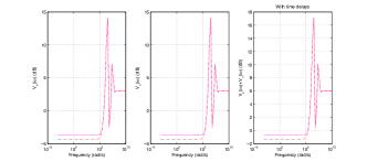
Figure 10: Performance of the system when the amplification loss coefficient is $\chi=5.5902\times 10^{6}$ Hz, transmission losses of 5%, and there are time delays $T=10^{-6}$ s and $T_{m}=2\times 10^{-6}$ s.

VII Conclusion

This paper has developed and studied a distributed entanglement generation scheme for two continuous-mode output Gaussian fields that are radiated by two spatially separated Gaussian oscillator systems. It is shown that a LQG measurement-feedback controller can be designed to enhance the EPR-like entanglement between the two output fields across a certain frequency range, even in the presence of important practical imperfections in the system. It is demonstrated that the controller displays a degree of robustness in the sense that although it was designed for the ideal scenario it can still provide an enhancement and stability over the case of no controller being present, despite the presence of the imperfections. In summary, the results reported here indicate the potential utility of feedback controllers in the task of distributed entanglement generation using distributed resources.

References

- (1) J. I. Cirac, P. Zoller, H. J. Kimble, and H. Mabuchi, Phys. Rev. Lett. 78, 3221 (1997).
- (2) C. W. Chou, J. Laurat, H. Deng, K. S. Choi, H. de Riedmatten, D. Felinto, and H. J. Kimble, Science 316, 1316 (2007).
- (3) C. H. Bennett, H. J. Bernstein, S. Popescu, and B. Schumacher, Phys. Rev. A 53, 2046 (1996).
- (4) A. Ferraro, S. Olivares, and M. G. A. Paris, e-print arXiv:quant-ph/0503237 (2005).
- (5) J. Eisert, S. Scheel, and M. B. Plenio, Phys. Rev. Lett. 89, 137903 (2002).
- (6) S. Mancini and H. M. Wiseman, Phys. Rev. A 75, 012330 (2007).
- (7) A. Serafini and S. Mancini, Phys. Rev. Lett. 104, 220501 (2010).
- (8) A. R. R. Carvalho, A. J. S. Reid, and J. J. Hope, Phys. Rev. A 78, 012334 (2008).
- (9) N. Yamamoto, H. I. Nurdin, M. R. James, and I. R. Petersen, Phys. Rev. A 78, 042339 (2008).
- (10) H. M. Wiseman and G. J. Milburn, Quantum Measurement and Control, (Cambridge University Press, 2010).
- (11) Z. Yan, X. Jia, C. Xie, and K. Peng, Phys. Rev. A 84, 062304 (2011).
- (12) A. C. Doherty and K. Jacobs, Phys. Rev. A 60, 2700 (1999).
- (13) V. P. Belavkin and S. C. Edwards, Quantum filtering and optimal control, in Quantum Stochastics and Information: Statistics, Filtering and Control, 143-205, (World Scientific, 2008).
- (14) C. W. Gardiner and P. Zoller, Quantum Noise, (Springer-Verlag, Berlin and New York, 3rd edition, 2004).
- (15) Z. Y. Ou, S. F . Pereira, and H. J. Kimble, Appl. Phys. B 55, 265 (1992).
- (16) D. Vitali, G. Morigi, and J. Eschner, Phys. Rev. A 74, 053814 (2006).
- (17) S. Iida, M. Yukawa, H. Yonezawa, N. Yamamoto, and A. Furusawa, IEEE Trans. Automat. Contr. 57(8), 2045-2050 (2012).
- (18) H. I. Nurdin, M. R. James, and A. C. Doherty, SIAM J. Control Optim. 48-4, 2686-2718 (2009).
- (19) J. Gough and M. R. James, IEEE Trans. Automat. Contr. 54-11, 2530-2544 (2009).
- (20) J. Gough and M. R. James, Comm. Math. Phys. 287, 1109-1132 (2009).
- (21) W. Michiels and S. I. Niculescu, Stability and Stabilization of Time-Delay Systems, (Advances in Design and Control, SIAM, 2007).
- (22) K. Engelborghs, T. Luzyanina, and G. Samaey, DDE-BIFTOOL vol. 2.00: A Matlab package for bifurcation analysis of delay differential equations, (Technical report TW-330, Department of Computer Science, Katholieke Universiteit Leuven, Leuven, Belgium, 2001).
- (23) K. Engelborghs, T. Luzyanina, and D. Roose, ACM Trans. Math. Softw. 28(1), 1-21 (2002).
- (24) D. Q. Cao, P. He, and K. Zhang, J. Math. Anal. Appl. 283, 362-374 (2003).
- (25) J. Lei and M. C. Mackey, SIAM J. Appl. Math 67, 387-407 (2007).
- (26) A. A. Moelja, G. Meinsma, and J. Kuipers, IEEE Transactions Automat. Contr. 51(8), 1347-1354 (2006).
- (27) K. Nishio, K. Kashima, and J. Imura, Phys. Rev. A 79, 062105 (2009).
- (28) C. Emary, e-print arXiv:1207.2910 [cond-mat.mes-hall] (2012).