Correlated variables in regression:
clustering and sparse estimation

Abstract

We consider estimation in a high-dimensional linear model with strongly correlated variables. We propose to cluster the variables first and do subsequent sparse estimation such as the Lasso for cluster-representatives or the group Lasso based on the structure from the clusters. Regarding the first step, we present a novel and bottom-up agglomerative clustering algorithm based on canonical correlations, and we show that it finds an optimal solution and is statistically consistent. We also present some theoretical arguments that canonical correlation based clustering leads to a better-posed compatibility constant for the design matrix which ensures identifiability and an oracle inequality for the group Lasso. Furthermore, we discuss circumstances where cluster-representatives and using the Lasso as subsequent estimator leads to improved results for prediction and detection of variables. We complement the theoretical analysis with various empirical results.

Keywords and phrases: Canonical correlation, group Lasso, Hierarchical clustering, High-dimensional inference, Lasso, Oracle inequality, Variable screening, Variable selection.

1 Introduction

High-dimensional regression is used in many fields of applications nowadays where the number of covariables $p$ greatly exceeds sample size $n$, i.e., $p\gg n$. We focus here on the simple yet useful high-dimensional linear model

$${\bf Y}={\bf X}\beta^{0}+{\boldsymbol{\varepsilon}},$$ (1)

with univariate $n\times 1$ response vector ${\bf Y}$, $n\times p$ design matrix ${\bf X}$, $p\times 1$ true underlying coefficient vector $\beta^{0}$ and $n\times 1$ error vector ${\boldsymbol{\varepsilon}}$. Our primary goal is to do variable screening for the active set, i.e., the support of $\beta^{0}$, denoted by $S_{0}=\{j;\ \beta^{0}_{j}\neq 0,\ j=1,\ldots p\}$: we want to have a statistical procedure $\hat{S}$ such that with high probability, $\hat{S}\supseteq S_{0}$ (and $|\hat{S}|$ not too large). In the case where $p\gg n$, the obvious difficulties are due to (near) non-identifiability. While some positive results have been shown under some assumptions on the design ${\bf X}$, see the paragraph below, high empirical correlation between variables or near linear dependence among a few variables remain as notorious problems which are often encountered in many applications. Examples include genomics where correlation and the degree of linear dependence is high within a group of genes sharing the same biological pathway (Segal et al.,, 2003), or genome-wide association studies where SNPs are highly correlated or linearly dependent within segments of the DNA sequence (Balding,, 2007).

An important line of research to infer the active set $S_{0}$ or for variable screening has been developed in the past using the Lasso (Tibshirani,, 1996) or versions thereof (Zou,, 2006; Meinshausen,, 2007; Zou and Li,, 2008). Lasso-type methods have proven to be successful in a range of practical problems. From a theoretical perspective, their properties for variable selection and screening have been established assuming various conditions on the design matrix ${\bf X}$, such as the neighborhood stability or irrepresentable condition (Meinshausen and Bühlmann,, 2006; Zhao and Yu,, 2006), and various forms of “restricted” eigenvalue conditions, see van de Geer, (2007); Zhang and Huang, (2008); Meinshausen and Yu, (2009); Bickel et al., (2009); van de Geer and Bühlmann, (2009); Sun and Zhang, (2011). Despite of these positive findings, situations where high empirical correlations between covariates or near linear dependence among a few covariables occur cannot be handled well with the Lasso: the Lasso tends to select only one variable from the group of correlated or nearly linearly dependent variables, even if many or all of these variables belong to the active set $S_{0}$. The elastic net (Zou and Hastie,, 2005), OSCAR (Bondell and Reich,, 2008) and “clustered Lasso” (She,, 2010) have been proposed to address this problem but they do not explicitly take correlation-structure among the variables into account and still exhibit difficulties when groups of variables are nearly linearly dependent. A sparse Laplacian shrinkage estimator has been proposed (Huang et al.,, 2011) and proven to select a correct set of variables under certain regularity conditions. However, the sparse Laplacian shrinkage estimator is geared toward the case where highly correlated variables have similar predictive effects (which we do not require here) and its selection consistency theorem necessarily requires a uniform lower bound for the nonzero signals above an inflated noise level due to model uncertainty.

We take here the point of view that we want to avoid false negatives, i.e., to avoid not selecting an active variable from $S_{0}$: the price to pay for this is an increase in false positive selections. From a practical point of view, it can be very useful to have a selection method $\hat{S}$ which includes all variables from a group of nearly linearly independent variables where at least one of them is active. Such a procedure is often a good screening method, when measured by $|\hat{S}\cap S_{0}|/|S_{0}|$ as a function of $|\hat{S}|$. The desired performance can be achieved by clustering or grouping the variables first and then selecting whole clusters instead of single variables.

1.1 Relation to other work and new contribution

The idea of clustering or grouping variables and then pursuing model fitting is not new, of course. Principal component regression (Kendall,, 1957, cf.) is among the earliest proposals, and Hastie et al., (2000) have used principal component analysis in order to find a set of highly correlated variables where the clustering can be supervised by a response variable. Tree-harvesting (Hastie et al.,, 2001) is another proposal which uses supervised learning methods to select groups of predictive variables formed by hierarchical clustering. An algorithmic approach, simultaneously performing the clustering and supervised model fitting, was proposed by Dettling and Bühlmann, (2004), and also the OSCAR method (Bondell and Reich,, 2008) does such simultaneous grouping and supervised model fitting.

Our proposal differs from previous work in various aspects. We primarily propose to use canonical correlation for clustering the variables as this reflects the notion of linear dependence among variables: and it is exactly this notion of linear dependence which causes the identifiability problems in the linear model in (1). Hence, this is conceptually a natural strategy for clustering variables when having the aim to address identifiability problems with variable selection in the linear model (1). We present in Section 2.1 an agglomerative hierarchical clustering method using canonical correlation, and we prove that it finds the finest clustering which satisfies the criterion function that between group canonical correlations are smaller than a threshold and that it is statistically consistent. Furthermore, we prove in Section 4.1 that the construction of groups based on canonical correlations leads to well-posed behavior of the group compatibility constant of the design matrix ${\bf X}$ which ensures identifiability and an oracle inequality for the group Lasso (Yuan and Lin,, 2006). The latter is a natural choice for estimation and cluster selection; another possibility is to use the Lasso for cluster representatives. We analyze both of these methods: this represents a difference to earlier work where at the time, such high-dimensional estimation techniques have been less or not established at all.

We present some supporting theory in Section 4, describing circumstances where clustering and subsequent estimation improves over standard Lasso without clustering, and the derivations also show the limitations of such an approach. This sheds light for what kind of models and scenarios the commonly used two-stage approach in practice, consisting of clustering variables first and subsequent estimation, is beneficial. Among the favorable scenarios which we will examine for the latter approach are: (i) high within cluster correlation and weak between cluster correlation with potentially many active variables per cluster; and (ii) at most one active variable per cluster where the clusters are tight (high within correlation) but not necessarily assuming low between cluster correlation. Numerical results which complement the theoretical results are presented in Section 5.

2 Clustering covariables

Consider the index set $\{1,\ldots,p\}$ for the covariables in (1). In the sequel, we denote by $x^{(j)}$ the $j$th component of a vector $x$ and by $X^{(G)}=\{X^{(j)};\ j\in G\}$ the group of variables from a cluster $G\subseteq\{1,\ldots,p\}$. The goal is to find a partition ${\cal G}$ into disjoint clusters $G_{1},\ldots,G_{q}$: ${\cal G}=\{G_{1},\ldots,G_{q}\}$ with $\cup_{r=1}^{q}G_{r}=\{1,\ldots,p\}$ and $G_{r}\cap G_{\ell}=\emptyset\ (r\neq\ell)$. The partition ${\cal G}$ should then satisfy certain criteria.

We propose two methods for clustering the variables, i.e., finding a suitable partition: one is a novel approach based on canonical correlations while the other uses standard correlation based hierarchical clustering.

2.1 Clustering using canonical correlations

For a partition ${\cal G}=\{G_{1},\ldots,G_{q}\}$ as above, we consider:

$$\hat{\rho}_{\mathrm{max}}({\cal G})=\max\{\hat{\rho}_{\mathrm{can}}(G_{r},G_{\ell});\ r,\ell\in\{1,\ldots,q\},\ r\neq\ell\}.$$

Here, $\hat{\rho}_{\mathrm{can}}(G_{r},G_{\ell})$ denotes the empirical canonical correlation (Anderson,, 1984, cf.) between the variables from $X^{(G_{r})}$ and $X^{(G_{\ell})}$. (The empirical canonical correlation is always non-negative). A clustering with $\tau$-separation between clusters is defined as:

$$\hat{{\cal G}}(\tau)=\mbox{a partition $\hat{{\cal G}}$ of $\{1,\ldots,p\}$ such that}\ \hat{\rho}_{\mathrm{max}}(\hat{{\cal G}})\leq\tau\ (0<\tau<1).$$ (2)

Not all values of $\tau$ are feasible: if $\tau$ is too small, then there is no partition which would satisfy (2). For this reason, we define the canonical correlation of all the variables with the empty set of variables as zero: hence, the trivial partition ${\cal G}_{\mathrm{single}}$ consisting of the single cluster $\{1,\ldots,p\}$ has $\hat{\rho}_{\mathrm{max}}({\cal G}_{\mathrm{single}})=0$ which satisfies (2). The fact that $\tau$ may not be feasible (except with ${\cal G}_{\mathrm{single}}$) can be understood from the view point that coarse partitions do not necessarily lead to smaller values of $\hat{\rho}_{\mathrm{max}}$: for example, when $p\gg n$ and if $\mathrm{rank}(X^{(G_{r}\cup G_{\ell})})=n$, which would typically happen if $|G_{r}\cup G_{\ell}|>n$, then $\hat{\rho}_{\mathrm{can}}(G_{r},G_{\ell})=1$. In general, clustering with $\tau$-separation does not have a unique solution. For example, if $\hat{{\cal G}}(\tau)=\{G_{1},\ldots,G_{q}\}$ is a clustering with $\tau$-separation and $\{G_{r;k},k=1,\ldots,q_{r}\}$ is a nontrivial partition of $G_{r}$ with $\max_{1\leq k_{1}<k_{2}\leq q_{r}}\hat{\rho}_{\mathrm{can}}(G_{r;k_{1}},G_{r;k_{2}})\leq\tau$, then $\{G_{1},\ldots,G_{r-1},G_{r;k},k=1,\ldots,q_{r},G_{r+1},\ldots,G_{q}\}$ is a strictly finer clustering with $\tau$-separation, see also Lemma 7.1 below. The non-uniqueness of clustering with $\tau$-separation motivates the following definition of the finest clustering with $\tau$-separation. A clustering with $\tau$-separation between clusters, say $\hat{{\cal G}}(\tau)$, is finest if every other clustering with $\tau$-separation is strictly coarser than $\hat{{\cal G}}(\tau)$, and we denote such a finest clustering with $\tau$-separation by

$$\hat{{\cal G}}_{\mathrm{finest}}(\tau).$$

The existence and uniqueness of the finest clustering with $\tau$-separation are provided in Theorem 2.1 below.

1:  Start with the single variables as $p$ clusters (nodes at the bottom of a tree). Set $b=0$

2:  repeat

3:     Increase $b$ by one. Merge the two clusters having highest canonical correlation.

4:  until Criterion (2) is satisfied.

Algorithm 1 Bottom-up, agglomerative hierarchical clustering using canonical correlations.

A simple hierarchical bottom-up agglomerative clustering (without the need to define linkage between clusters) can be used as an estimator $\hat{\cal G}(\tau)$ which satisfies (2) and which is finest: the procedure is described in Algorithm 1.

Theorem 2.1

The hierarchical bottom-up agglomerative clustering Algorithm 1 leads to a partition $\hat{\cal G}(\tau)$ which satisfies (2). If $\tau$ is not feasible with a nontrivial partition, the solution is the coarsest partition $\hat{\cal G}(\tau)={\cal G}_{\mathrm{single}}=\{G\}$ with $G=\{1,\ldots,p\}$.

Furthermore, if $\tau$ is feasible with a nontrivial partition, the solution ${\hat{\cal G}}(\tau)=\hat{\cal G}_{\mathrm{finest}}(\tau)$ is the finest clustering with $\tau$-separation.

A proof is given in Section 7. Theorem 2.1 describes that a bottom-up greedy strategy leads to an optimal solution.

We now present consistency of the clustering Algorithm 1. Denote the population canonical correlation between $X^{(G_{r})}$ and $X^{(G_{\ell})}$ by $\rho_{\mathrm{can}}(G_{r},G_{\ell})$, and the maximum population canonical correlation by $\max_{r\neq\ell}\rho_{\mathrm{can}}(G_{r},G_{\ell})$, respectively, for a partition ${\cal G}=\{G_{1},\ldots,G_{q}\}$ of $\{1,\ldots,p\}$. As in (2), a partition ${\cal G}(\tau)$ is a population clustering with $\tau$-separation if $\rho_{\max}(\cal G)\leq\tau$. The finest population clustering with $\tau$-separation, denoted by ${\cal G}_{\mathrm{finest}}(\tau)$, is the one which is finer than any other population clustering with $\tau$-separation. With the convention $\rho_{\max}({\cal G}_{\mathrm{single}})=0$, the existence and uniqueness of the finest population clustering with $\tau$-separation follows from Theorem 2.1. In fact, the hierarchical bottom-up agglomerative clustering Algorithm 1 yields the finest population clustering ${\cal G}_{\mathrm{finest}}(\tau)$ with $\tau$-separation if the population canonical correlation is available and used in the algorithm.

Let ${\cal G}_{\mathrm{finest}}(\tau)$ be the finest population clustering with $\tau$-separation and ${\hat{\cal G}}(\tau)$ be the sample clustering with $\tau$-separation generated by the hierarchical bottom-up agglomerative clustering Algorithm 1 based on the design matrix ${\bf X}$. The following theorem provides a sufficient condition for the consistency of ${\hat{\cal G}}(\tau)$ in the Gaussian model

$$X_{1},\ldots,X_{n}\ \mbox{i.i.d.}\ \sim{\cal N}_{p}(0,\Sigma).$$ (3)

For any given $t>0$ and positive integers $q$ and $d_{1},\ldots,d_{q}$, define

$$t_{r}=\sqrt{d_{r}/n}+\sqrt{(2/n)(t+\log(q(q+1))},\ \Delta_{r,\ell}^{*}=\frac{3(t_{r}\wedge t_{\ell})+(t_{r}\vee t_{\ell})}{(1-t_{r})(1-t_{\ell})}.$$ (4)

Theorem 2.2

Consider ${\bf X}$ from (3) and ${\cal G}^{0}=\{G_{1},\ldots,G_{q}\}$ a partition of $\{1,\ldots,p\}$. Let $t>0$ and $d_{r}=\mathrm{rank}(\Sigma_{G_{r},G_{r}})$. Define $\Delta^{*}_{r,\ell}$ by (4). Suppose

$$\max_{1\leq r<\ell\leq q}\big{\{}\rho_{\mathrm{can}}(G_{r},G_{\ell})+\Delta^{*}_{r,\ell}\big{\}}\leq\tau_{-}\leq\tau_{+}$$ (5)

$$< \min_{1\leq r\leq q}\min_{\{G_{r;k}\}}\big{\{}\max_{k_{1}<k_{2}}\rho_{\mathrm{can}}(G_{r;k_{1}},G_{r;k_{2}})-\Delta^{*}_{r,r}\big{\}},$$

where $\min_{\{G_{r;k}\}}$ is taken over all nontrivial partitions $\{G_{r;k},k\leq q_{r}\}$ of $G_{r}$. Then, ${\cal G}^{0}={\cal G}_{\mathrm{finest}}(\tau)$ is the finest population clustering with $\tau$-separation for all $\tau_{-}\leq\tau\leq\tau_{+}$, and

$$\mathbb{P}[{\hat{\cal G}}(\tau)={\cal G}_{\mathrm{finest}}(\tau),\ \forall\tau_{-}\leq\tau\leq\tau_{+}\Big{]}\geq 1-\exp(-t).$$

A proof is given in Section 7. We note that $t=\sqrt{\log(p)}$ leads to $t_{r}\asymp\sqrt{\mathrm{rank}(\Sigma_{G_{r},G_{r}})/n}+\sqrt{\log(p)/n}$: this is small if $\mathrm{rank}(\Sigma_{G_{r},G_{r}})=o(n)$ and $\log(p)=o(n)$, and then, $\Delta^{*}_{r,\ell}$ is small as well (which means that the probability bound becomes $1-p^{-1}\to 1\ (p\to\infty)$ (or $p\geq n\to\infty$).

The parameter $\tau$ in (2) needs to be chosen. We advocate the use of the minimal resulting $\tau$. This can be easily implemented: we run the bottom-up agglomerative clustering Algorithm 1 and record in every iteration the maximal canonical correlation between clusters, denoted by $\hat{\rho}_{\max}(b)$ where $b$ is the iteration number. We then use the partition corresponding to the iteration

$$\hat{b}=\mathop{\arg\min}\limits_{b}\hat{\rho}_{\mathrm{max}}(b).$$ (6)

A typical path of $\hat{\rho}_{\mathrm{max}}(b)$ as a function of the iterations $b$, the choice $\hat{b}$ and the corresponding minimal $\hat{\rho}_{\max}(\hat{b})$ are shown in Figure 1.

Figure 1: Path of $\hat{\rho}_{\mathrm{max}}(b)$ as a function of the iterations $b$: from real data described in Section 5.2 with $p=1000$ and $n=71$.

We conclude that the hierarchical bottom-up agglomerative clustering Algorithm 1 with the rule in (6) is fully data-driven, and there is no need to define linkage between clusters.

2.2 Ordinary hierarchical clustering

As an alternative to the clustering method in Section 2.1, we consider in Section 5.2 ordinary hierarchical agglomerative clustering based on the dissimilarity matrix $D$ with entries $D_{r,\ell}=1-|\hat{\rho}(X^{(r)},X^{(\ell)})|$, where $\hat{\rho}(X^{(r)},X^{(\ell)})$ denotes the sample correlation between $X^{(r)}$ and $X^{(\ell)}$. We choose average-linkage as dissimilarity between clusters.

As a cutoff for determining the number of clusters, we proceed according to an established principle. In every clustering iteration $b$, proceeding in an agglomerative way, we record the new value $h_{b}$ of the corresponding linkage function from the merged clusters (in iteration $b$): we then use the partition corresponding to the iteration

$$\hat{b}=\mathop{\arg\max}\limits_{b}(h_{b+1}-h_{b}).$$

3 Supervised selection of clusters

From the design matrix ${\bf X}$, we infer the clusters $G_{1},\ldots,G_{q}$ as described in Section 2. We select the variables in the linear model (1) in a group-wise fashion where all variables from a cluster $G_{r}$ ($r=1,\ldots,q$) are selected or not: this is denoted by

$$\hat{S}_{\mathrm{cluster}}=\{r;\ \mbox{cluster $G_{r}$ is selected},\ r=1,\ldots,q\}.$$

The selected set of variables is then the union of the selected clusters:

$$\hat{S}=\cup_{r\in\hat{S}_{\mathrm{cluster}}}G_{r}.$$ (7)

We propose two methods for selecting the clusters, i.e., two different estimators $\hat{S}_{\mathrm{cluster}}$.

3.1 Cluster representative Lasso (CRL)

For each cluster we consider the representative

$$\bar{{\bf X}}^{(r)}=\frac{1}{|G_{r}|}\sum_{j\in G_{r}}{\bf X}^{(j)},\ r=1,\ldots,q,$$

where ${\bf X}^{(j)}$ denotes the $j$th $n\times 1$ column-vector of ${\bf X}$. Denote by $\bar{{\bf X}}$ the $n\times q$ design matrix whose $r$th column is given by $\bar{{\bf X}}^{(r)}$. We use the Lasso based on the response ${\bf Y}$ and the design matrix $\bar{{\bf X}}$:

$$\hat{\beta}_{\mathrm{CRL}}=\mathop{\arg\min}\limits_{\beta}(\|{\bf Y}-\bar{{\bf X}}\beta\|_{2}^{2}/n+\lambda_{\mathrm{CRL}}\|\beta\|_{1}).$$

The selected clusters are then given by

$$\hat{S}_{\mathrm{cluster,CRL}}=\hat{S}_{\mathrm{cluster,CRL}}(\lambda_{\mathrm{CRL}})=\{r;\ \hat{\beta}_{\mathrm{CRL},r}(\lambda_{\mathrm{CRL}})\neq 0,\ r=1,\ldots,q\},$$

and the selected variables are obtained as in (7), denoted as

$$\hat{S}_{\mathrm{CRL}}=\hat{S}_{\mathrm{CRL}}(\lambda_{\mathrm{CRL}})=\cup_{r\in\hat{S}_{\mathrm{cluster,CRL}}}G_{r}.$$

3.2 Cluster group Lasso (CGL)

Another obvious way to select clusters is given by the group Lasso. We partition the vector of regression coefficients according to the clusters: $\beta=(\beta_{G_{1}},\ldots,\beta_{G_{q}})^{T}$, where $\beta_{G_{r}}=(\{\beta_{j};\ j\in G_{r}\})^{T}$. The cluster group Lasso is defined as

$$\hat{\beta}_{\mathrm{CGL}}=\mathop{\arg\min}\limits_{\beta}\|{\bf Y}-{\bf X}\beta\|_{2}^{2}/n+\lambda_{\mathrm{CGL}}\sum_{r=1}^{q}w_{r}\|{\bf X}^{(G_{r})}\beta_{G_{r}}\|_{2}n^{-1/2},$$ (8)

where $w_{r}$ is a multiplier, typical pre-specified as $w_{r}=\sqrt{|G_{r}|}$. It is well known that the group Lasso enjoys a group selection property where either $\hat{\beta}_{\mathrm{CGL},G_{r}}\neq 0$ (all components are different from zero) or $\hat{\beta}_{\mathrm{CGL},G_{r}}\equiv 0$ (the zero-vector). We note that the estimator in (8) is different from using the usual penalty $\lambda\sum_{r=1}^{q}w_{r}\|\beta_{G_{r}}\|_{2}$: the penalty in (8) is termed as “groupwise prediction penalty” in Bühlmann and van de Geer, (2011, Sec.4.5.1): it has nice parameterization invariance properties, and it is a much more appropriate penalty when ${\bf X}^{(G_{r})}$ exhibits strongly correlated columns.

The selected clusters are then given by

$$\hat{S}_{\mathrm{cluster,CGL}}=\hat{S}_{\mathrm{cluster,CGL}}(\lambda_{\mathrm{CGL}})=\{r;\ \hat{\beta}_{\mathrm{CGL},G_{r}}(\lambda_{\mathrm{CGL}})\neq 0,\ r=1,\ldots,q\},$$

and the selected variables are as in (7):

$$\hat{S}_{\mathrm{CGL}}=\hat{S}_{\mathrm{CGL}}(\lambda_{\mathrm{CGL}})=\cup_{r\in\hat{S}_{\mathrm{cluster,CGL}}}G_{r}=\{j;\ \hat{\beta}_{\mathrm{CGL},j}\neq 0,\ j=1,\ldots,p\},$$

where the latter equality follows from the group selection property of the group Lasso.

4 Theoretical results for cluster Lasso methods

We provide here some supporting theory, first for the cluster group Lasso (CGL) and then for the cluster representative Lasso (CRL).

4.1 Cluster group Lasso (CGL)

We will show first that the compatibility constant of the design matrix ${\bf X}$ is well-behaved if the canonical correlation between groups is small, i.e., a situation which the clustering Algorithm 1 is exactly aiming for.

The CGL method is based on the whole design matrix ${\bf X}$, and we can write the model in group structure form where we denote by ${\bf X}^{(G_{r})}$ the $n\times|G_{r}|$ design matrix with variables $\{{\bf X}^{(j)};\ j\in G_{r}\}$:

$${\bf Y}={\bf X}\beta^{0}+{\boldsymbol{\varepsilon}}=\sum_{r=1}^{q}{\bf X}^{(G_{r})}\beta^{0}_{G_{r}}+{\boldsymbol{\varepsilon}},$$ (9)

where $\beta^{0}_{G_{r}}=(\{\beta_{j}^{0};\ j\in G_{r}\})^{T}$. We denote by $S_{0,\mathrm{Group}}=\{r;\ \beta_{G_{r}}^{0}\neq 0,\ r=1,\ldots,q\}$.

We introduce now a few other notations and definitions. We let $m_{r}:=|G_{r}|$, $r=1,\ldots,q$, denote the group sizes, and define the average group size

$$\bar{m}:={1\over q}\sum_{r=1}^{q}m_{r},$$

and the average size of active groups

$$\bar{m}_{S_{0,{\rm Group}}}:={1\over|S_{0,{\rm Group}}|}\sum_{r\in S_{0,{\rm Group}}}m_{r}.$$

Furthermore, for any $S\subseteq\{1,\ldots,q\}$, we let ${\bf X}^{(S)}$ be the design matrix containing the variables in $\cup_{r\in S}G_{r}$. Moreover, define

$$\|\beta_{S}\|_{2,1}:=\sum_{r\in S}\|{\bf X}^{(G_{r})}\beta_{G_{r}}\|_{2}\sqrt{m_{r}/\bar{m}}.$$

We denote in this section by

$$\hat{\Sigma}_{r,\ell}:=({\bf X}^{(G_{r})})^{T}{\bf X}^{(G_{\ell})}/n,\ r,\ell\in\{1,\ldots,q\}.$$

We assume that each $\hat{\Sigma}_{r,r}$ is non-singular (otherwise one may use generalized inverses) and we write, assuming here for notational clarity that $S_{0,{\rm Group}}=\{1,\ldots,s_{0}\}$ ($s_{0}=|S_{0,{\rm Group}}|$) is the set of indices of the first $s_{0}$ groups:

$$\hat{R}_{S_{0,{\rm Group}}}:=\left(\begin{array}[]{cccc}I&\hat{\Sigma}_{1,1}^{-1/2}\hat{\Sigma}_{1,2}\hat{\Sigma}_{2,2}^{-1/2}&\cdots&\hat{\Sigma}_{1,1}^{-1/2}\hat{\Sigma}_{1,s_{0}}\hat{\Sigma}_{s_{0},s_{0}}^{-1/2}\\ \hat{\Sigma}_{2,2}^{-1/2}\hat{\Sigma}_{2,1}\hat{\Sigma}_{1,1}^{-1/2}&I&\cdots&\hat{\Sigma}_{2,2}^{-1/2}\hat{\Sigma}_{2,s_{0}}\hat{\Sigma}_{s_{0},s_{0}}^{-1/2}\\ \vdots&\vdots&\ddots&\vdots\\ \hat{\Sigma}_{s_{0},s_{0}}^{-1/2}\hat{\Sigma}_{s_{0},1}\hat{\Sigma}_{1,1}^{-1/2}&\hat{\Sigma}_{s_{0},s_{0}}^{-1/2}\hat{\Sigma}_{s_{0},2}\hat{\Sigma}_{2,2}^{-1/2}&\cdots&I\end{array}\right).$$

The group compatibility constant given in Bühlmann and van de Geer, (2011) is a value $\phi_{0,{\rm Group}}^{2}({\bf X})$ that satisfies

$$\phi_{0,{\rm Group}}^{2}({\bf X})\leq\min\biggl{\{}{\bar{m}_{S_{0}}|S_{0,{\rm Group}}|\over\bar{m}}{\|{\bf X}\beta\|_{2}^{2}\over\|\beta_{S_{0,{\rm Group}}}\|_{2,1}^{2}};\ \|\beta_{S_{0,{\rm Group}}^{c}}\|_{2,1}\leq\|\beta_{S_{0,{\rm Group}}}\|_{2,1}\biggr{\}}.$$

The constant 3 here is related to the condition $\lambda\geq 2\lambda_{0}$ in Proposition 4.1 below: in general it can be taken as $(\lambda+\lambda_{0})/(\lambda-\lambda_{0})$.

Theorem 4.1

Suppose that $\hat{R}_{S_{0,{\rm Group}}}$ has smallest eigenvalue $\hat{\Lambda}_{\rm min}^{2}>0$. Assume moreover the incoherence conditions:

$$\rho:=\max_{r\in S_{0},\ell\in S_{0}^{c}}{\bar{m}\over\sqrt{m_{r}m_{\ell}}}{\hat{\rho}_{\rm can}(G_{r},G_{\ell})}\leq C{\hat{\Lambda}_{\rm min}^{2}\bar{m}/\bar{m}_{S_{0,{\rm Group}}}\over 3|S_{0,{\rm Group}}|}\ \ \mbox{for some}\ 0<C<1,$$

$$\rho_{S_{0,{\rm Group}}}:=\max_{r,\ell\in S_{0,{\rm Group}},\ r\neq\ell}{\bar{m}\over\sqrt{m_{r}m_{\ell}}}{\hat{\rho}_{\rm can}(G_{r},G_{\ell})}<{1\over|S_{0,{\rm Group}}|}.$$

Then, the group Lasso compatibility holds with compatibility constant

$$\phi_{0,{\rm Group}}^{2}({\bf X}) \geq {\biggl{(}\hat{\Lambda}_{\rm min}^{2}\bar{m}/\bar{m}_{S_{0,{\rm Group}}}-3|S_{0,{\rm Group}}|\rho\biggr{)}^{2}/\biggl{(}{\hat{\Lambda}_{\rm min}^{2}\bar{m}^{2}/\bar{m}_{S_{0,{\rm Group}}}^{2}}}\biggr{)}$$

$$\geq (1-C)^{2}\hat{\Lambda}_{\rm min}^{2}\geq(1-C)^{2}(1-|S_{0,{\rm Group}}|\rho_{S_{0,{\rm Group}}})$$

$$> 0.$$

A proof is given in Section 7. We note that small enough canonical correlations between groups ensure the incoherence assumptions for $\rho$ and $\rho_{S_{0,{\rm Group}}}$, and in turn that the group Lasso compatibility condition holds. The canonical correlation based clustering Algorithm 1 is tailored for this situation.

Remark 1. One may in fact prove a group version of Corollary 7.2 in Bühlmann and van de Geer, (2011) which says that under the eigenvalue and incoherence condition of Theorem 4.1, a group irrepresentable condition holds. This in turn implies that, with large probability, the group Lasso will have no false positive selection of groups, i.e., one has a group version of the result of Problem 7.5 in Bühlmann and van de Geer, (2011).

Known theoretical results can then be applied for proving an oracle inequality of the group Lasso.

Proposition 4.1

Consider model (1) with fixed design ${\bf X}$ and Gaussian error ${\boldsymbol{\varepsilon}}\sim{\cal N}_{n}(0,\sigma^{2}I)$. Let

$$\lambda_{0}=\sigma\frac{2}{\sqrt{n}}\sqrt{1+\sqrt{\frac{4t+4\log(p)}{m_{\mathrm{min}}}}+\frac{4t+4\log(p)}{m_{\mathrm{min}}}},$$

where $m_{\mathrm{min}}=\min_{r=1,\ldots,q}|m_{r}|$. Assume that $\hat{\Sigma}_{r,r}$ is non-singular,for all $r=1,\ldots,q$. Then, for the group Lasso estimator $\hat{\beta}(\lambda)$ in (8) with $\lambda\geq 2\lambda_{0}$, and with probability at least $1-\exp(-t)$:

$$\|{\bf X}(\hat{\beta}(\lambda)-\beta^{0})\|_{2}^{2}/n+\lambda\sum_{r=1}^{q}\sqrt{m_{r}}\|\hat{\beta}_{G_{r}}(\lambda)-\beta_{G_{r}}^{0}\|_{2}\leq 24\lambda^{2}\sum_{r\in S_{0,\mathrm{{Group}}}}m_{r}/\phi_{0,\mathrm{Group}}^{2}({\bf X}),$$ (11)

where $\phi_{0,\mathrm{Group}}^{2}({\bf X})$ denotes the group compatibility constant.

Proof: We can invoke the result in Bühlmann and van de Geer, (2011, Th.8.1): using the groupwise prediction penalty in (8) leads to an equivalent formalization where we can normalize to $\hat{\Sigma}_{r,r}=I_{m_{r}\times m_{r}}$. The requirement $\lambda\geq 4\lambda_{0}$ in Bühlmann and van de Geer, (2011, Th.8.1) can be relaxed to $\lambda\geq 2\lambda_{0}$ since the model (1) is assumed to be true, see also Bühlmann and van de Geer, (2011, p.108,Sec.6.2.3). $\Box$

4.2 Linear dimension reduction and subsequent Lasso estimation

For a mean zero Gaussian random variable $Y\in\mathbb{R}$ and a mean zero Gaussian random vector $X\in\mathbb{R}^{p}$, we can always use a random design Gaussian linear model representation:

$$Y=\sum_{j=1}^{p}\beta^{0}_{j}X^{(j)}+\varepsilon,$$

$$X\sim{\cal N}_{p}(0,\Sigma),\ \varepsilon\sim{\cal N}(0,\sigma^{2}),$$ (12)

where $\varepsilon$ is independent of $X$.

Consider a linear dimension reduction

$$Z=A_{q\times p}X$$

using a matrix $A_{q\times p}$ with $q<p$. We denote in the sequel by

$$\mu_{X}=\mathbb{E}[Y|X]=\sum_{j=1}^{p}\beta^{0}_{j}X^{(j)},\ \ \mu_{Z}=\mathbb{E}[Y|Z]=\sum_{r=1}^{q}\gamma^{0}_{r}Z^{(r)}.$$

Of particular interest is $Z=(\bar{X}^{(1)},\ldots,\bar{X}^{(q)})^{T}$, corresponding to the cluster representatives $\bar{X}^{(r)}=|G_{r}|^{-1}\sum_{j\in G_{r}}X^{(j)}$. Due to the Gaussian assumption in (4.2), we can always represent

$$Y=\sum_{r=1}^{q}\gamma^{0}_{r}Z^{(r)}+\eta=\mu_{Z}+\eta,$$ (13)

where $\eta$ is independent of $Z$. Furthermore, since $\mu_{Z}$ is the linear projection of $Y$ on the linear span of $Z$ and also the linear projection of $\mu_{X}$ on the linear span of $Z$,

$$\xi^{2}=\mathrm{Var}(\eta)=\mathrm{Var}(\varepsilon+\mu_{X}-\mu_{Z})=\sigma^{2}+\mathbb{E}[(\mu_{X}-\mu_{Z})^{2}].$$

For the prediction error, when using the dimension-reduced $Z$ and for any estimator $\hat{\gamma}$, we have, using that $\mu_{X}-\mu_{Z}$ is orthogonal to the linear span of $Z$:

$$\mathbb{E}[(X^{T}\beta^{0}-Z^{T}\hat{\gamma})^{2}]=\mathbb{E}[(Z^{T}\gamma^{0}-Z^{T}\hat{\gamma})^{2}]+\mathbb{E}[(\mu_{X}-\mu_{Z})^{2}].$$ (14)

Thus, the total prediction error consists of an error due to estimation of $\gamma^{0}$ and a squared bias term $B^{2}=\mathbb{E}[(\mu_{X}-\mu_{Z})^{2}]$. The latter has already appeared in the variance $\xi^{2}=\mathrm{Var}(\eta)$ above.

Let ${\bf Y},\ {\bf X}$ and ${\bf Z}$ be $n$ i.i.d. realizations of the variables $Y,X$ and $Z$, respectively. Then,

$${\bf Y}={\bf X}\beta^{0}+{\boldsymbol{\varepsilon}}={\bf Z}\gamma^{0}+{\boldsymbol{\eta}}.$$

Consider the Lasso, applied to ${\bf Y}$ and ${\bf Z}$, for estimating $\gamma^{0}$:

$$\hat{\gamma}=\mbox{argmin}_{\gamma}(\|{\bf Y}-{\bf Z}\gamma\|_{2}^{2}/n+\lambda\|\gamma\|_{1}).$$

The cluster representative Lasso (CRL) is a special case with $n\times q$ design matrix ${\bf Z}=\bar{{\bf X}}$.

Proposition 4.2

Consider $n$ i.i.d. realizations from the model (4.2). Let

$$\lambda_{0}=2\|\hat{\sigma}_{{\bf Z}}\|_{\infty}\xi\sqrt{\frac{t^{2}+2\log(q)}{n}},$$

where $\|\hat{\sigma}_{{\bf Z}}\|_{\infty}=\max_{r=1,\ldots,q}\sqrt{(n^{-1}{\bf Z}^{T}{\bf Z})_{rr}}$, and $\xi^{2}=\sigma^{2}+\mathbb{E}[(\mu_{X}-\mu_{Z})^{2}]$. Then, for $\lambda\geq 2\lambda_{0}$ and with probability at least $1-2\exp(-t^{2}/2)$, conditional on ${\bf Z}$:

$$\|{\bf Z}(\hat{\gamma}-\gamma^{0})\|_{2}^{2}/n+\lambda\|\hat{\gamma}-\gamma^{0}\|_{1}\leq 4\lambda^{2}s(\gamma^{0})/\phi_{0}^{2}({\bf Z}),$$

where $s(\gamma^{0})$ equals the number of non-zero coefficients in $\gamma^{0}$ and $\phi_{0}^{2}({\bf Z})$ denotes the compatibility constant of the design matrix ${\bf Z}$ (Bühlmann and van de Geer,, 2011, (6.4)).

A proof is given in Section 7. The choice $\lambda=2\lambda_{0}$ leads to the convergence rates:

$$\|{\bf Z}(\hat{\gamma}(\lambda)-\gamma^{0})\|_{2}^{2}/n=O_{P}\Big{(}\frac{s(\gamma^{0})\log(q)}{n\phi_{0}^{2}({\bf Z})}\Big{)},$$

$$\|\hat{\gamma}(\lambda)-\gamma^{0}\|_{1}=O_{P}\Big{(}\frac{s(\gamma^{0})}{\phi_{0}^{2}({\bf Z})}\sqrt{\frac{\log(q)}{n}}\Big{)}.$$ (15)

The second result about the $\ell_{1}$-norm convergence rate implies a variable screening property as follows: assume a so-called beta-min condition requiring that

$$\min_{r\in S(\gamma^{0})}|\gamma^{0}_{r}|\geq Cs(\gamma^{0})\sqrt{\frac{\log(q)}{n}}/\phi_{0}^{2}({\bf Z})$$ (16)

for a sufficiently large $C>0$, then, with high probability, $\hat{S}_{{\bf Y},{\bf Z}}(\lambda)\supseteq S(\gamma^{0})$, where $\hat{S}_{{\bf Y},{\bf Z}}(\lambda)=\{r;\ \hat{\gamma}_{r}(\lambda)\neq 0\}$ and $S(\gamma^{0})=\{r;\ \gamma^{0}_{r}\neq 0\}$.

The results in Proposition 4.2, (4.2) and (16) describe inference for ${\bf Z}\gamma^{0}$ and for $\gamma^{0}$. Their meaning for inferring ${\bf X}\beta^{0}$ and for (groups) of $\beta^{0}$ are further discussed in Section 4.3 for specific examples, representing $\gamma^{0}$ in terms of $\beta^{0}$ and the correlation structure of $X$, and analyzing the squared bias $B^{2}=\mathbb{E}[(\mu_{X}-\mu_{Z})^{2}]$. The compatibility constant $\phi_{0}^{2}({\bf Z})$ in Proposition 4.2 is typically (much) better behaved, if $q\ll p$, than the corresponding constant $\phi_{0}^{2}({\bf X})$ of the original design ${\bf X}$. Bounds of $\phi_{0}^{2}({\bf X})$ and $\phi_{0}^{2}({\bf Z})$ in terms of their population covariance $\Sigma$ and $A\Sigma A^{T}$, respectively, can be derived from Bühlmann and van de Geer, (2011, Cor.6.8). Thus, loosely speaking, we have to deal with a trade-off: the term $\phi_{0}^{2}({\bf Z})$, coupled with a $\log(q)$- instead of a $\log(p)$-factor (and also to a certain extent the sparsity factor $s(\gamma^{0})$) are favorable for the dimensionality reduced ${\bf Z}$. The price to pay for this is the bias term $B^{2}=\mathbb{E}[(\mu_{X}-\mu_{Z})^{2}]$, discussed further in Section 4.3, which appears in the variance $\xi^{2}$ entering the definition of $\lambda_{0}$ in Proposition 4.2 as well as in the prediction error (14); furthermore, the detection of $\gamma^{0}$ instead of $\beta^{0}$ can be favorable for some cases and not favorable for others, as discussed in Section 4.3.

Finally, note that Proposition 4.2 makes a statement conditional on ${\bf Z}$: with high probability $1-\alpha$,

$$\mathbb{P}[\|{\bf Z}\hat{\gamma}-{\bf Z}\gamma^{0}\|_{2}^{2}/n\leq 4\lambda^{2}s(\gamma^{0})/\phi_{0}^{2}({\bf Z})|{\bf Z}]\geq 1-\alpha.$$

Assuming that $\phi_{0}^{2}({\bf Z})\geq\phi_{0}^{2}(A,\Sigma)$ is bounded with high probability (Bühlmann and van de Geer,, 2011, Lem.6.17), we obtain (for a small but different $\alpha$ than above):

$$\mathbb{P}[\|{\bf Z}\hat{\gamma}-{\bf Z}\gamma^{0}\|_{2}^{2}/n\leq 4\lambda^{2}s(\gamma^{0})/\phi_{0}^{2}(A,\Sigma)]\geq 1-\alpha.$$

In view of (14), we then have for the prediction error:

$$\mathbb{E}[\|{\bf X}\beta^{0}-{\bf Z}\hat{\gamma}\|_{2}^{2}/n]=\mathbb{E}[\|{\bf Z}\hat{\gamma}-{\bf Z}\gamma^{0}\|_{2}^{2}/n+\mathbb{E}[(\mu_{X}-\mu_{Z})^{2}],$$ (17)

where $\mathbb{E}[\|{\bf Z}\hat{\gamma}-{\bf Z}\gamma^{0}\|_{2}^{2}/n]\approx O(\xi s(\gamma^{0})\sqrt{\log(p)/n})$ when choosing $\lambda=2\lambda_{0}$.

4.3 The parameter $\gamma^{0}$ for cluster representatives

In the sequel, we consider the case where $Z=\bar{X}=(\bar{X}^{(1)},\ldots,\bar{X}^{(q)})^{T}$ encodes the cluster representatives $\bar{X}^{(r)}=|G_{r}|^{-1}\sum_{j\in G_{r}}X^{(j)}$. We analyze the coefficient vector $\gamma^{0}$ and discuss it from the view-point of detection. For specific examples, we also quantify the squared bias term $B^{2}=\mathbb{E}[(\mu_{X}-\mu_{\bar{X}})^{2}]$ which plays mainly a role for prediction.

The coefficient $\gamma^{0}$ can be exactly described if the cluster representatives are independent.

Proposition 4.3

Consider a random design Gaussian linear model as in (4.2) where $\mathrm{Cov}(\bar{X}^{(r)},\bar{X}^{(\ell)})=0$ for all $r\neq\ell$. Then,

$$\gamma_{r}^{0}=|G_{r}|\sum_{j\in G_{r}}w_{j}\beta^{0}_{j},\ r=1,\ldots,q,$$

$$w_{j}=\frac{\sum_{k=1}^{p}\Sigma_{j,k}}{\sum_{\ell\in G_{r}}\sum_{k=1}^{p}\Sigma_{\ell,k}},\ \ \sum_{j\in G_{r}}w_{j}=1.$$

Moreover:

1. If, for $r\in\{1,\ldots,q\}$, $\Sigma_{j,k}\geq 0$ for all $j,k\in G_{r}$, then $w_{j}\geq 0\ (j\in G_{r})$, and $\gamma^{0}_{r}/|G_{r}|$ is a convex combination of $\beta_{j}^{0}\ (j\in G_{r})$. In particular, if $\beta^{0}_{j}\geq 0$ for all $j\in G_{r}$, or $\beta^{0}_{j}\leq 0$ for all $j\in G_{r}$, then

   $$|\gamma^{0}_{r}|\geq|G_{r}|\min_{j\in G_{r}}|\beta^{0}_{j}|.$$

2. If, for $r\in\{1,\ldots,q\}$, $\Sigma_{j,j}\equiv 1$ for all $j\in G_{r}$ and $\sum_{k\neq j}\Sigma_{j,k}\equiv\zeta$ for all $j\in G_{r}$, then $w_{j}\equiv|G_{r}|^{-1}$ and

   $$\gamma^{0}_{r}=\sum_{j\in G_{r}}\beta^{0}_{j}.$$

   A concrete example is where $\Sigma$ has a block-diagonal structure with equi-correlation within blocks: $\Sigma_{j,k}\equiv\rho_{r}\ (j,k\in G_{r},\ j\neq k)$ with $-1/(|G_{r}|-1)<\rho_{r}<1$ (where the lower bound for $\rho_{r}$ ensures positive definiteness of the block-matrix $\Sigma_{G_{r},G_{r}}$).

A proof is given in Section 7. The assumption of uncorrelatedness across $\{\bar{X}^{(r)};\ r=1,\ldots,q\}$ is reasonable if we have tight clusters corresponding to blocks of a block-diagonal structure of $\Sigma$.

We can immediately see that there are benefits or disadvantages of using the group representatives in terms of the size of the absolute value $|\gamma_{r}^{0}|$: obviously a large value would make it easier to detect the group $G_{r}$. Taking a group representative is advantageous if all the coefficients within a group have the same sign. However, we should be a bit careful since the size of a regression coefficient should be placed in context to the standard deviation of the regressor: here, the standardized coefficients are

$$\gamma^{0}_{r}\sqrt{\mathrm{Var}(\bar{X}^{(r)})}.$$ (18)

For e.g. high positive correlation among variables within a group, $\mathrm{Var}(\bar{X}^{(r)})$ is much larger than for independent variables: for the equi-correlation scenario in statement 2. of Proposition 4.3 we obtain for the standardized coefficient

$$\gamma_{r}^{0}\sqrt{\mathrm{Var}(\bar{X}^{(r)})}=\sum_{j\in G_{r}}\beta^{0}_{j}\sqrt{\rho+|G_{r}|^{-1}(1-\rho)}\approx\sum_{j\in G_{r}}\beta^{0}_{j},$$ (19)

where the latter approximation holds if $\rho\approx 1$.

The disadvantages occur if rough or near cancellation among $\beta_{j}^{0}\ (j\in G_{r})$ takes place. This can cause a reduction of the absolute value of $|\gamma^{0}_{r}|$ in comparison to $\max_{j\in G_{r}}|\beta_{j}^{0}|$: again, the scenario in statement 2. of Proposition 4.3 is most clear in the sense that the sum of $\beta^{0}_{j}\ (j\in G_{r})$ is equal to $\gamma^{0}_{r}$, and near cancellation would mean that $\sum_{j\in G_{r}}\beta_{j}^{0}\approx 0$.

An extension of Proposition 4.3 can be derived for covering the case where the regressors $\{\bar{X}^{(r)};\ r=1,\ldots,q\}$ are only approximately uncorrelated.

Proposition 4.4

Assume the conditions of Proposition 4.3 but instead of uncorrelatedness of $\{\bar{X}^{(r)};\ r=1,\ldots,q\}$ across $r$, we require: for $r\in\{1,\ldots,q\}$,

$$|\mathrm{Cov}(X^{(i)},X^{(j)}|\{\bar{X}^{(\ell)};\ \ell\neq r\})|\leq\nu\ \mbox{for all}\ j\in G_{r},\ i\notin G_{r}.$$

Moreover, assume that $\mathrm{Var}(\bar{X}^{(r)}|\{\bar{X}^{(\ell)};\ \ell\neq r\})\geq C>0$. Then,

$$\gamma_{r}^{0}=|G_{r}|\sum_{j\in G_{r}}w_{j}\beta^{0}_{j}+\Delta_{r},\ |\Delta_{r}|\leq\nu\|\beta^{0}\|_{1}/C.$$

Furthermore, if $\mathrm{Cov}(X^{(i)},X^{(j)}|\{\bar{X}^{(\ell)};\ \ell\neq r\})\geq 0$ for all $j\in G_{r},\ i\notin G_{r}$, and $\mathrm{Var}(\bar{X}^{(r)}|\{\bar{X}^{(k)};\ k\neq r\})\geq C>0$, then:

$$|\gamma_{r}^{0}|\geq|G_{r}|\min_{j\in G_{r}}|\beta^{0}_{j}|+\Delta_{r},\ |\Delta_{r}|\leq\nu\|\beta^{0}\|_{1}/C.$$

A proof is given in Section 7. The assumption that $|\mathrm{Cov}(X^{(i)},X^{(j)}|\{\bar{X}^{(k)};\ k\neq r\})|\leq\nu$ for all $j\in G_{r},\ i\notin G_{r}$ is implied if the variables in $G_{r}$ and $G_{\ell}\ (r\neq\ell)$ are rather uncorrelated. Furthermore, if we require that $\nu\|\beta^{0}\|_{1}\ll|G_{r}|\min_{j\in G_{r}}|\beta^{0}_{j}|$ and $C\asymp 1$ (which holds if $\Sigma_{j,j}\equiv 1$ for all $j\in G_{r}$ and if the variables within $G_{r}$ have high conditional correlations given $\{\bar{X}^{(\ell)};\ \ell\neq r\}$), then:

$$|\gamma^{0}_{r}|\geq|G_{r}|\min_{j\in G_{r}}|\beta^{0}_{j}|(1+o(1)).$$

Thus, also under clustering with only moderate independence between the clusters, we can have beneficial behavior for the representative cluster method. This also implies that the representative cluster method works if the clustering is only approximately correct, as shown in Section 4.6.

We discuss in the next subsections two examples in more detail.

4.3.1 Block structure with equi-correlation

Consider a partition with groups $G_{r}\ (r=1,\ldots,q)$. The population covariance matrix $\Sigma$ is block-diagonal having $|G_{r}|\times|G_{r}|$ block-matrices $\Sigma_{G_{r},G_{r}}$ with equi-correlation: $\Sigma_{j,j}\equiv 1$ for all $j\in G_{r}$, and $\Sigma_{j,k}\equiv\rho_{r}$ for all $j,k\in G_{r}\ (j\neq k)$, where $-1/(|G_{r}|-1)<\rho_{r}<1$ (the lower bound for $\rho_{r}$ ensures positive definiteness of $\Sigma_{G_{r},G_{r}}$). This is exactly the setting as in statement 2. of Proposition 4.3.

The parameter $\gamma^{0}$ equals, see Proposition 4.3:

$$\gamma_{r}^{0}=\sum_{j\in G_{r}}\beta^{0}_{j}.$$

Regarding the bias, observe that

$$\mu_{X}-\mu_{\bar{X}}=\sum_{r=1}^{q}(\mu_{X;r}-\mu_{\bar{X};r}),$$

where $\mu_{X;r}=\sum_{j\in G_{r}}\beta^{0}_{j}X^{(j)}$ and $\mu_{\bar{X};r}=\bar{X}^{(r)}\gamma^{0}_{r}$, and due to block-independence of $X$, we have

$$\mathbb{E}[(\mu_{X}-\mu_{\bar{X}})^{2}]=\sum_{r=1}^{q}\mathbb{E}[(\mu_{X;r}-\mu_{\bar{X};r})^{2}].$$

For each summand, we have $\mu_{X;r}-\mu_{\bar{X};r}=\sum_{j\in G_{r}}X^{(j)}(\beta^{0}_{j}-\bar{\beta}^{0}_{r})$, where $\bar{\beta}^{0}_{r}=|G_{r}|^{-1}\times$
$\sum_{j\in G_{r}}\beta^{0}_{j}$. Thus,

$$\mathbb{E}[(\mu_{X;r}-\mu_{\bar{X};r})^{2}] = \sum_{j\in G_{r}}(\beta^{0}_{j}-\bar{\beta}^{0}_{r})^{2}+2\rho_{r}\sum_{j,k\in G_{r};j\neq k}(\beta^{0}_{j}-\bar{\beta}^{0}_{r})(\beta^{0}_{k}-\bar{\beta}^{0}_{r})$$

$$= (1-\rho_{r})\sum_{j\in G_{r}}(\beta^{0}_{j}-\bar{\beta}^{0}_{r})^{2}.$$

Therefore, the squared bias equals

$$B^{2}=\mathbb{E}[(\mu_{X;r}-\mu_{\bar{X};r})^{2}]=\sum_{r=1}^{q}(1-\rho_{r})\sum_{j\in G_{r}}(\beta^{0}_{j}-\bar{\beta}^{0}_{r})^{2}.$$ (20)

We see from the formula that the bias is small if there is little variation of $\beta^{0}$ within the groups $G_{r}$ or/and the $\rho_{r}$’s are close to one. The latter is what we obtain with tight clusters: there is a large within and small between groups correlation. Somewhat surprising is the fact that the bias is becoming large if $\rho_{r}$ tends to negative values (which is related to the fact that detection becomes bad for negative values of $\rho_{r}$, see (19)).

Thus, in summary: in comparison to an estimator based on ${\bf X}$, using the cluster representatives $\bar{{\bf X}}$ and subsequent estimation leads to equal (or better, due to smaller dimension) prediction error if all $\rho_{r}$’s are close to 1, regardless of $\beta^{0}$. When using the cluster representative Lasso, if $B^{2}=\sum_{r=1}^{q}(1-\rho_{r})\sum_{j\in G_{r}}(\beta^{0}_{j}-\bar{\beta}^{0}_{r})^{2}=O(s(\gamma^{0})\log(q)/n)$, then the squared bias has no disturbing effect on the prediction error as can be seen from (4.2).

With respect to detection, there can be a substantial gain for inferring the cluster $G_{r}$ if $\beta^{0}_{j}\ (j\in G_{r})$ have all the same sign, and if $\rho_{r}$ is close to 1. Consider the active groups

$$S_{0,\mathrm{Group}}=\{r;\ \beta^{0}_{G_{r}}\neq 0,\ r=1,\ldots,q\}.$$

For the current model and assuming that $\sum_{j\in G_{r}}\beta^{0}_{j}\neq 0\ (r=1,\ldots,q)$ (i.e., no exact cancellation of coefficients within groups), $S_{0,\mathrm{Group}}=S(\gamma^{0})=\{r;\ \gamma^{0}_{r}\neq 0\}$. In view of (19) and (16), the screening property for groups holds if

$$\min_{r\in S_{0,\mathrm{Group}}}|\sum_{j\in G_{r}}\beta^{0}_{j}\sqrt{\rho+|G_{r}|^{-1}(1-\rho)}|\geq C\frac{s(\gamma^{0})}{\phi_{0}^{2}(\bar{{\bf X}})}\sqrt{\frac{\log(q)}{n}}.$$

This condition holds even if the non-zero $\beta^{0}_{j}$’s are very small but their sum within a group is sufficiently strong.

4.3.2 One active variable per cluster

We design here a model with at most one active variable in each group. Consider a low-dimensional $q\times 1$ variable $U$ and perturbed versions of $U^{(r)}\ (r=1,\ldots,q)$ which constitute the $p\times 1$ variable $X$:

$$X^{(r,1)}=U^{(r)},\ r=1,\ldots,q,$$ (21)

$$X^{(r,j)}=U^{(r)}+\delta^{(r,j)},\ j=2,\ldots,m_{r},\ r=1,\ldots,q,$$

$$\delta^{(r,2)},\ldots,\delta^{(r,m_{r})}\ \mbox{i.i.d.}\ {\cal N}(0,\tau_{r}^{2})\ \mbox{and independent among}\ r=1,\ldots,q.$$

The index $j=1$ has no specific meaning, and the fact that one covariate is not perturbed is discussed in Remark 2 below. The purpose is to have at most one active variable in every cluster by assuming a low-dimensional underlying linear model

$$Y=\sum_{r=1}^{q}\tilde{\beta}^{0}_{r}U^{(r)}+\varepsilon,$$ (22)

where $\varepsilon\sim{\cal N}(0,\sigma^{2})$ is independent of $U$. Some of the coefficients in $\tilde{\beta}^{0}$ might be zero, and hence, some of the $U^{(r)}$’s might be noise covariates. We construct a $p\times 1$ variable $X$ by stacking the variables $X^{(r,j)}$ as follows: $X^{(\sum_{\ell=1}^{r-1}m_{\ell}+j)}=X^{(r,j)}\ (j=1,\ldots,m_{r})$ for $r=1,\ldots,q$. Furthermore, we use an augmented vector of the true regression coefficients

$$\beta^{0}_{j}=\left\{\begin{array}[]{ll}\tilde{\beta}^{0}_{r}&\mbox{if $j=\sum_{\ell=1}^{r-1}m_{\ell}+1,\ r=1,\ldots,q$},\\ 0&\mbox{otherwise}.\end{array}\right.$$

Thus, the model in (22) can be represented as

$$Y=\sum_{j=1}^{p}\beta^{0}_{j}X^{(j)}+\varepsilon,$$

where $\varepsilon$ is independent of $X$.

Remark 2. Instead of the model in (21)–(22), we could consider

$$X^{(r,j)}=U^{(r)}+\delta^{(r,j)},\ j=1,\ldots,m_{r},\ r=1,\ldots,q,$$

$$\delta^{(r,1)},\ldots,\delta^{(r,m_{r})}\ \mbox{i.i.d.}\ {\cal N}(0,\tau_{r}^{2})\ \mbox{and independent among}\ r=1,\ldots,q,$$

and

$$Y=\sum_{j=1}^{p}\beta^{0}_{j}X^{(j)}+\varepsilon,$$

where $\varepsilon$ is independent of $X$. Stacking the variables $X^{(r,j)}$ as before, the covariance matrix $\mathrm{Cov}(X)$ has $q$ equi-correlation blocks but the blocks are generally dependent if $U^{(1)},\ldots,U^{(q)}$ are correlated, i.e., $\mathrm{Cov}(X)$ is not of block-diagonal form. If $\mathrm{Cov}(U^{(r)},U^{(\ell)})=0\ (r\neq\ell)$, we are back to the model in Section 4.3.1. For more general covariance structures of $U$, an analysis of the model seems rather cumbersome (but see Proposition 4.4) while the analysis of the “asymmetric” model (21)-(22) remains rather simple as discussed below.

We assume that the clusters $G_{r}$ are corresponding to the variables $\{X^{(r,j)};\ j=1,\ldots,m_{r}\}$ and thus, $m_{r}=|G_{r}|$. In contrast to the model in Section 4.3.1, we do not assume uncorrelatedness or quantify correlation between clusters. The cluster representatives are

$$\bar{X}^{(r)}=m_{r}^{-1}\sum_{j\in G_{r}}X^{(r,j)}=U^{(r)}+W^{(r)},$$

$$W^{(r)}\sim{\cal N}(0,\tau_{r}^{2}\frac{m_{r}-1}{m_{r}^{2}})\ \mbox{and independent among}\ r=1,\ldots,q.$$

As in (13), the dimension-reduced model is written as $Y=\sum_{r=1}^{q}\gamma_{r}^{0}\bar{X}^{(r)}+\eta$.

For the bias, we immediately find:

$$B^{2} = \mathbb{E}[(\mu_{X}-\mu_{\bar{X}})^{2}]$$ (24)

$$\leq \mathbb{E}[(U^{T}\tilde{\beta}^{0}-\bar{X}\tilde{\beta}^{0})^{2}]=\mathbb{E}|W^{T}\tilde{\beta}^{0}|^{2}\leq s_{0}\max_{j}|\beta^{0}_{j}|^{2}\max_{r}\frac{m_{r}-1}{m_{r}^{2}}\tau_{r}^{2}.$$

Thus, if the cluster sizes $m_{r}$ are large and/or the perturbation noise $\tau_{r}^{2}$ is small, the squared bias $B^{2}$ is small.

Regarding detection, we make use of the following result.

Proposition 4.5

For the model in (22) we have:

$$\|\tilde{\beta}^{0}-\gamma^{0}\|_{2}^{2}\leq 2B^{2}/\lambda_{\mathrm{min}}^{2}(\mathrm{Cov}(U))=2\mathbb{E}|W^{T}\tilde{\beta}^{0}|^{2}/\lambda_{\mathrm{min}}^{2}(\mathrm{Cov}(U))$$

$$\leq 2s_{0}\max_{j}|\beta^{0}_{j}|^{2}\max_{r}\frac{m_{r}-1}{m_{r}^{2}}\tau_{r}^{2}/\lambda_{\mathrm{min}}^{2}(\mathrm{Cov}(U)),$$

where $\lambda_{\mathrm{min}}^{2}(\mathrm{Cov}(U))$ denotes the minimal eigenvalue of $\mathrm{Cov}(U)$.

A proof is given in Section 7. Denote by $\tilde{S}_{0}=\{r;\ \tilde{\beta}^{0}_{r}\neq 0\}$. We then have:

if $$\ \min_{r\in\tilde{S}_{0}}|\tilde{\beta}^{0}_{r}|>2\sqrt{2s_{0}\max_{j}|\beta^{0}_{j}|\max_{r}\frac{m_{r}-1}{m_{r}^{2}}\tau_{r}^{2}/\lambda_{\mathrm{min}}^{2}(\mathrm{Cov}(U))},$$ (25)

then: $$\ \min_{r\in\tilde{S}_{0}}|\gamma^{0}_{r}|>\sqrt{2s_{0}\max_{j}|\beta^{0}_{j}|\max_{r}\frac{m_{r}-1}{m_{r}^{2}}\tau_{r}^{2}/\lambda_{\mathrm{min}}^{2}(\mathrm{Cov}(U))}.$$

This follows immediately: if the implication would not hold, it would create a contradiction to Proposition 4.5.

We argue now that

$$\max_{r}\frac{\tau_{r}^{2}}{m_{r}}=O(\log(q)/n)$$ (26)

is a sufficient condition to achieve prediction error and detection as in the $q$-dimensional model (22). Thereby, we implicitly assume that $\max_{j}|\beta_{j}^{0}|\leq C<\infty$ and $\lambda_{\mathrm{min}}^{2}(\mathrm{Cov}(U))\geq L>0$. Since we have that $s(\gamma^{0})\geq s_{0}$ (excluding the pathological case for a particular combination of $\beta^{0}$ and $\Sigma=\mathrm{Cov}(X)$), using (24) the condition (26) implies

$$B^{2}=O(s_{0}\log(q)/n)\leq O(s(\gamma^{0})\log(q)/n)$$

which is at most of the order of the prediction error in (4.2), where $\phi_{0}^{2}({\bf Z})=\phi_{0}^{2}(\bar{{\bf X}})$ can be lower-bounded by the population version $\phi_{0}^{2}(\mathrm{Cov}(\bar{X}))\geq\phi_{0}^{2}(\mathrm{Cov}(U))$ (Bühlmann and van de Geer,, 2011, Cor.6.8). For detection, we note that (26) implies that the bound in (25) is at most

$$\min_{r\in\tilde{S}_{0}}|\gamma^{0}_{r}|>\sqrt{2s_{0}\max_{j}|\beta^{0}_{j}|\max_{r}\frac{m_{r}-1}{m_{r}^{2}}\tau_{r}^{2}/\lambda_{\mathrm{min}}^{2}(\mathrm{Cov}(U))}\leq O(s(\gamma^{0})\sqrt{\log(q)/n}).$$

The right-hand side is what we require as beta-min condition in (16) for group screening such that with high probability $\hat{S}\supseteq S(\gamma^{0})\supseteq S_{0}$ (again excluding a particular constellation of $\beta^{0}$ and $\Sigma$).

The condition (26) itself is fulfilled if $m_{r}\asymp n/\log(q)$, i.e., when the cluster sizes are large, or if $\tau_{r}^{2}=O(\log(q)/n)$, i.e., the clusters are tight. An example where the model (21)–(22) with (26) seems reasonable is for genome-wide association studies with SNPs where $p\approx 10^{6}$, $n\approx 1000$ and $m_{r}$ can be in the order of $10^{3}$ and hence $q\approx 1000$ when e.g. using the order of magnitude of number of target SNPs (Carlson et al.,, 2004). Note that this is a scenario where the group sizes $m_{r}\gg n$ where the cluster group Lasso seems inappropriate.

The analysis in Sections 4.2 and 4.3 about the bias $B^{2}$ and the parameter $\gamma^{0}$ has immediate implications for the cluster representative Lasso (CRL), as discussed in the next section.

4.4 A comparison

We compare now the results of the cluster representative Lasso (CRL), the cluster group Lasso (CGL) and the plain Lasso, at least on a “rough scale”.

For the plain Lasso we have: with high probability,

$$\|{\bf X}(\hat{\beta}_{\mathrm{Lasso}}-\beta^{0})\|_{2}^{2}/n=O\Big{(}\frac{\log(p)s_{0}}{n\phi_{0}^{2}({\bf X})}\Big{)},$$

$$\|\hat{\beta}_{\mathrm{Lasso}}-\beta^{0}\|_{1}=O\Big{(}\frac{s_{0}}{\phi_{0}^{2}({\bf X})}\sqrt{\frac{\log(p)}{n}}\Big{)},$$ (27)

which both involve $\log(p)$ instead of $\log(q)$ and more importantly, the compatibility constant $\phi_{0}^{2}({\bf X})$ of the ${\bf X}$ design matrix instead of $\phi_{0}^{2}(\bar{{\bf X}})$ of the matrix $\bar{{\bf X}}$. If $p$ is large, then $\phi_{0}^{2}({\bf X})$ might be close to zero; furthermore, it is exactly in situations like model (21) and (22), having a few ($s_{0}\leq q$) active variables and noise covariates being highly correlated with the active variables, which leads to very small values of $\phi_{0}^{2}({\bf X})$, see van de Geer and Lederer, (2011). For variable screening $\hat{S}_{\mathrm{Lasso}}(\lambda)\supseteq S_{0}$ with high probability, the corresponding (sufficient) beta-min condition is

$$\min_{j\in S_{0}}|\beta^{0}_{j}|\geq Cs_{0}\sqrt{\frac{\log(p)}{n}}/\phi_{0}^{2}({\bf X})$$ (28)

for a sufficiently large $C>0$.

For comparison with the cluster group Lasso (CGL) method, we assume for simplicity equal group sizes $|G_{r}|=m_{r}\equiv m$ for all $r$ and $\log(q)/m\leq 1$, i.e., the group size is sufficiently large. We then obtain: with high probability,

$$\|{\bf X}(\hat{\beta}_{\mathrm{CGL}}-\beta^{0})\|_{2}^{2}/n=O\Big{(}\frac{|S_{0,\mathrm{Group}}|m}{n\phi_{0,\mathrm{Group}}^{2}({\bf X})}\Big{)},$$

$$\sum_{r=1}^{q}\|\hat{\beta}_{G_{r}}-\beta_{G_{r}}^{0}\|_{2}=O\Big{(}\frac{|S_{0,\mathrm{Group}}|\sqrt{m}}{\sqrt{n}\phi_{0,\mathrm{Group}}^{2}({\bf X})}\Big{)}.$$ (29)

For variable screening $\hat{S}_{\mathrm{CGL}}(\lambda)\supseteq S_{0}$ with high probability, the corresponding (sufficient) beta-min condition is

$$\min_{r\in S_{0,\mathrm{Group}}}\|\beta_{G_{r}}^{0}\|_{2}\geq C\frac{|S_{0,\mathrm{Group}}|\sqrt{m}}{\sqrt{n}\phi_{0,\mathrm{Group}}^{2}({\bf X})}$$

for a sufficiently large $C>0$. The compatibility constants $\phi_{0}^{2}({\bf X})$ in (4.4) and $\phi_{0,\mathrm{Group}}^{2}({\bf X})$ in (4.4) are not directly comparable, but see Theorem 4.1 which is in favor of the CGL method. “On the rough scale”, we can distinguish two cases: if the group-sizes are large with only none or a few active variables per group, implying $s_{0}=|S_{0}|\approx|S_{0,\mathrm{Group}}|$, the Lasso is better than the CGL method because the CGL rate involves $|S_{0,\mathrm{Group}}|m$ or $|S_{0,\mathrm{Group}}|\sqrt{m}$, respectively, instead of the sparsity $s_{0}$ appearing in the rate for the standard Lasso; for the case where we have either none or many active variables within groups, the CGL method is beneficial, mainly for detection, since $|S_{0,\mathrm{Group}}|m\approx|S_{0}|=s_{0}$ but $|S_{0,\mathrm{Group}}|\sqrt{m}<|S_{0}|=s_{0}$. The behavior in the first case is to be expected since in the group Lasso representation (9), the parameter vectors $\beta_{G_{r}}^{0}$ are very sparse within groups, and this sparsity is not exploited by the group Lasso. A sparse group Lasso method (Friedman et al., 2010a, ) would address this issue. On the other hand, the CGL method has the advantage that it works without bias, in contrast to the CRL procedure. Furthermore, the CGL can also lead to good detection if many $\beta_{j}^{0}$’s in a group are small in absolute value. For detection of the group $G_{r}$, we only need that $\|\beta_{G_{r}}^{0}\|_{2}$ is sufficiently large: the signs of the coefficients of $\beta_{G_{r}}$ can be different and (near) cancellation does not happen.

For the cluster representative Lasso (CRL) method, the range of scenarios, with good performance of CRL, is more restricted. The method works well and is superior over the plain Lasso (and group Lasso) if the bias $B^{2}$ is small and the detection is well-posed in terms of the dimension-reduced parameter $\gamma^{0}$. More precisely, if

$$B^{2}=O\Big{(}\frac{s(\gamma^{0})\log(q)}{n\phi_{0}^{2}(\bar{{\bf X}})}\Big{)},$$

the CRL is better than plain Lasso for prediction since the corresponding oracle inequality for the CRL becomes, see (17): with high probability,

$$\|\bar{{\bf X}}\hat{\gamma}-{\bf X}\beta^{0}\|_{2}^{2}/n+\lambda\|\hat{\gamma}-\gamma^{0}\|_{1}\leq O\Big{(}\frac{s(\gamma^{0})\log(q)}{n\phi_{0}(\bar{{\bf X}})}\Big{)}.$$

We have given two examples and conditions ensuring that the bias is small, namely (20) and (26). The latter condition (26) is also sufficient for better screening property in the model from Section 4.3.2. For the equi-correlation model in Section 4.3.1, the success of screening crucially depends on whether the coefficients from active variables in a group nearly cancel or add-up (e.g. when having the same sign), see Propositions 4.3 and 4.4. The following Table 1 recapitulates the findings.

model	assumption	predict.	screen.
equi-corr. blocks (Sec. 4.3.1)	small value in (20)	+	NA
equi-corr. blocks (Sec. 4.3.1)	e.g. same sign for $\beta^{0}_{j}\ (j\in G_{r})$	NA	+
$\leq 1$ var. per group (Sec. 4.3.2)	(26)	+	+

Table 1: Comparison of cluster representative Lasso (CRL) with plain Lasso in terms of prediction and variable screening. The symbol “+” encodes better theoretical results for the CRL in comparison to Lasso; an “NA” means that no comparative statement can be made.

Summarizing, both the CGL and CRL are useful and can be substantially better than plain Lasso in terms of prediction and detection in presence of highly correlated variables. If the cluster sizes are smaller than sample size, the CGL method is more broadly applicable, in the sense of consistency but not necessarily efficiency, as it does not involve the bias term $B^{2}$ and constellation of signs or of near cancellation of coefficients in $\beta_{G_{r}}^{0}$ is not an issue. For group sizes which are larger than sample size, the CGL is not appropriate: one would need to take a version of the group Lasso with regularization within groups (Meier et al.,, 2009; Friedman et al., 2010a, ). The CGL method benefits when using canonical correlation based clustering as this improves the compatibility constant, see Theorem 4.1. The CRL method is particularly suited for problems where the variables can be grouped into tight clusters and/or the cluster sizes are large. There is gain if there is at most one active variable per cluster and the clusters are tight, otherwise the prediction performance is influenced by the bias $B^{2}$ and detection is depending on whether the coefficients within a group add-up or exhibit near cancellation. If the variables are not very highly correlated within large groups, the difficulty is to estimate these groups, and in case of correct grouping, as assumed in the theoretical results above, the CRL method may still perform (much) better than plain Lasso.

4.5 Estimation of the clusters

The theoretical derivations above assume that the groups $G_{r}\ (r=1,\ldots,q)$ correspond to the correct clusters. For the canonical correlation based clustering as in Algorithm 1, Theorem 2.2 discusses consistency in finding the true underlying population clustering. For hierarchical clustering, the issue is much simpler.

Consider the $n\times p$ design matrix ${\bf X}$ as in (3) and assume for simplicity that $\Sigma_{j,j}=1$ for all $j$. It is well-known that

$$\max_{j,k}|\hat{\Sigma}_{j,k}-\Sigma_{j,k}|=O_{P}(\sqrt{\log(p)/n}),$$ (30)

where $\hat{\Sigma}$ is the empirical covariance matrix (Bühlmann and van de Geer,, 2011, cf. p.152). Tightness and separation of the true clusters is ensured by:

$$\min\{|\Sigma_{j,k}|;\ j,k\ \in G_{r}\ (j\neq k),\ r=1,\ldots q\}$$ (31)

$$> \max\{|\Sigma_{j,k}|:\ j\in G_{r},\ k\in G_{\ell},\ r,\ell=1,\ldots,q\ (r\neq\ell)\}.$$

Assuming (31) and using (30), a standard clustering algorithm, using e.g. single-linkage and dissimilarity $1-|\hat{\Sigma}_{j,k}|$ between variables $X^{(j)}$ and $X^{(k)}$, will consistently find the true clusters if $\log(p)/n\to 0$.

In summary, and rather obvious: the higher the correlation within and uncorrelatedness between clusters, the better we can estimate the true underlying grouping. In this sense, and following the arguments in Sections 4.1–4.4, strong correlation within clusters “is a friend” when using cluster Lasso methods, while it is “an enemy” (at least for variable screening and selection) for plain Lasso.

4.6 Some first illustrations

We briefly illustrate some of the points and findings mentioned above for the CRL and the plain Lasso. Throughout this subsection, we show the results from a single realization of each of different models. More systematic simulations are shown in Section 5. We analyze scenarios with $p=1000$ and $n=100$. Thereby, the covariates are generated as in model (21) where $U\sim{\cal N}_{q}(0,I)$ with $q=5$ and $\tau=0.5$, and thus, $\mathrm{Cov}(X)=\Sigma$ is of block-diagonal structure. The response is as in the linear model (1) with ${\boldsymbol{\varepsilon}}\sim{\cal N}_{n}(0,I)$. We consider the following.

Correct and incorrect clustering. The correct clustering consists of $q=5$ clusters each having $m_{r}=|G_{r}|\equiv 200$ variables, corresponding to the structure in model (21). An incorrect clustering was constructed as 5 clusters where the first half (100) of the variables in each constructed cluster correspond to the first half (100) of the variables in each of the true 5 clusters, and the remaining second half (100) of the variables in the constructed clusters are chosen randomly from the total of 500 remaining variables. We note that $m_{r}\equiv 200>n=100$ and thus, the CGL method is inappropriate (see e.g. Proposition 4.1).

Active variables and regression coefficients. We always consider 3 active groups (a group is called active if there is at least one active variables in the group). The scenarios are as follows:

1. One active variable within each of 3 active groups, namely $S_{0}=\{1,201,401\}$. The regression coefficients are $\beta^{0}_{1}=-1,\ \beta^{0}_{201}=-1,\ \beta^{0}_{401}=1$;

2. 4 active variables within each of 3 active groups, namely $S_{0}=\{1,2,3,4,201,202,$
   $203,204,401,402,403,404\}$. The regression coefficients are $\beta^{0}_{j}\equiv 0.25$ for $j\in S_{0}$;

3. as in (b) but with regression coefficients $\{\beta^{0}_{j};\ j\in S_{0}\}\ \mbox{i.i.d.}\ \sim\mathrm{Unif}([-0.5,0.5]$;

4. as in (b) but with exact cancellation of coefficients: $\beta^{0}_{1}=\beta^{0}_{3}=2$, $\beta^{0}_{2}=\beta^{0}_{4}=-2$, $\beta^{0}_{201}=\beta^{0}_{203}=2$, $\beta^{0}_{202}=\beta^{0}_{204}=-2$, $\beta^{0}_{401}=\beta^{0}_{403}=2$, $\beta^{0}_{402}=\beta^{0}_{404}=-2$.

For the scenario in (d), we had to choose large coefficients, in absolute value equal to 2, in order to see clear differences, in favor of the plain Lasso. Figure 2, using the R-package glmnet (Friedman et al., 2010b, ) shows the results.

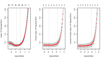
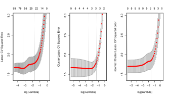
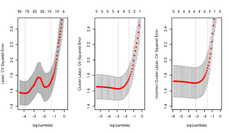
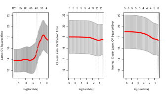
Figure 2: Left, middle and right panel of each subfigure: Lasso, cluster representative Lasso with correct clustering, and cluster representative Lasso with incorrect clustering as described in Section 4.6: 10-fold CV squared error (y-axis) versus $\log(\lambda)$ (x-axis). Grey bars indicate the region 10-fold CV squared error $+/-$ estimated standard error (s.e.) of 10-fold CV squared error. The left vertical bar indicates the minimizer of the CV error and the right vertical bar corresponds to the largest value such that the CV error is within one standard deviation (s.d.) of the minimum. The numbers on top of each plot report the number of selected variables (in case of the cluster representative Lasso, the number of selected representatives): the number of active groups is always equal to 3, and the number of active variables is 3 for (a) and 12 for (b)-(d). Subfigures (a)-(d) correspond to the scenarios (a)-(d) in Section 4.6.

The results seem rather robust against approximate cancellation of coefficients (Subfigure 2(c)) and incorrect clustering (right panels in Figure 2). Regarding the latter, the number of chosen clusters is worse than for correct clustering, though. A main message of the results in Figure 2 is that the predictive performance (using cross-validation) is a good indicator whether the group representative Lasso (with correct or incorrect clustering) works.

We can complement the rules from Section 2 for determining the number of clusters as follows: take the representative cluster Lasso method with the largest clusters (the least refined partition of $\{1,\ldots,p\}$) such that predictive performance is still reasonable (in comparison to the best achieved performance where we would always consider plain Lasso among the competitors as well). In the extreme case of Subfigure 2(d), this rule would choose the plain Lasso (among the alternatives of correct clustering and incorrect clustering) which is indeed the least refined partition such that predictive performance is still reasonable.

5 Numerical results

In this section we look at three different simulation settings and a pseudo real data example in order to empirically compare the proposed cluster Lasso methods with plain Lasso.

5.1 Simulated data

Here, we only report results for the CRL and CGL methods where the clustering of the variables is based on canonical correlations using Algorithm 1 (see Section 2.1). The corresponding results using ordinary hierarchical clustering, based on correlations and with average-linkage (see Section 2.2), are almost exactly the same because for the considered simulation settings, both clustering methods produce essentially the same partition.

We simulate data from the linear model in (1) with fixed design ${\bf X}$, ${\boldsymbol{\varepsilon}}\sim{\cal N}_{n}(0,\sigma^{2}I)$ with $n=100$ and $p=1000$. We generate the fixed design matrix ${\bf X}$ once, from a multivariate normal distribution $\mathcal{N}_{p}(0,\Sigma)$ with different structures for $\Sigma$, and we then keep it fixed. We consider various scenarios, but the sparsity or size of the active set is always equal to $s_{0}=20$.

In order to compare the various methods, we look at two performance measures for prediction and variable screening. For each model, our simulated data consists of a training and an independent test set. The models were fitted on the training data and we computed the test set mean squared error $n^{-1}\sum_{i=1}^{n}\mathbb{E}[(Y_{\mathrm{test}}(X_{i})-\hat{Y}(X_{i}))^{2}]$, denoted by MSE. For variable screening we consider the true positive rate as a measure of performance, i.e., $|\hat{S}\cap S_{0}|/|S_{0}|$ as a function of $|\hat{S}|$.

For each of the methods we choose a suitable grid of values for the tuning parameter. All reported results are based on 50 simulation runs.

5.1.1 Block diagonal model

Consider a block diagonal model where we simulate the covariables $X\sim\mathcal{N}_{p}(0,\Sigma_{A})$ where $\Sigma_{A}$ is a block diagonal matrix. We use a $10\times 10$ matrix $\Gamma$, where

$$\Gamma_{i,j}=\begin{cases}1,&i=j,\\ 0.9,&\text{else}.\end{cases}$$

The block-diagonal of $\Sigma_{A}$ consists of 100 such block matrices $\Gamma$. Regarding the regression parameter $\beta^{0}$, we consider the following configurations:

• $S_{0}=\{1,2,\ldots,20\}$ and for any $j\in S_{0}$ we sample $\beta^{0}_{j}$ from the set $\{2/s_{0},4/s_{0},\ldots,2\}$ without replacement (anew in each simulation run).

• $S_{0}=\{1,2,11,12,21,22,\dots,91,92\}$ and for any $j\in S_{0}$ we sample $\beta^{0}_{j}$ from the set $\{2/s_{0},4/s_{0},\ldots,2\}$ without replacement (anew in each simulation run).

• $\beta^{0}$ as in (Aa) but we switch the sign of half and randomly chosen active parameters (anew in each simulation run).

• $\beta^{0}$ as in (Ab) but we switch the sign of half and randomly chosen active parameters (anew in each simulation run).

The set-up (Aa) has all the active variables in the first two blocks of highly correlated variables. In the second configuration (Ab), the first two variables of each of the first ten blocks are active. Thus, in (Aa), half of the active variables appear in the same block while in the other case (Ab), the active variables are distributed among ten blocks. The remaining two configurations (Ac) and (Ad) are modifications in terms of random sign changes. The models (Ab) and (Ad) come closest to the model (22)-(21) considered for theoretical purposes: the difference is that the former models have two active variables per active block (or group) while the latter model has only one active variable per active group.

Table 2 and Figure 3 describe the simulation results.

$\sigma$	Method	(Aa)	(Ab)	(Ac)	(Ad)
	CRL	10.78 (1.61)	15.57 (2.43)	13.08 (1.65)	15.39 (2.35)
3	CGL	14.97 (2.40)	37.05 (5.21)	13.34 (2.06)	24.31 (6.50)
	Lasso	11.94 (1.97)	16.23 (2.47)	12.72 (1.67)	15.34 (2.53)
	CRL	161.73 (25.74)	177.90 (25.87)	157.86 (20.63)	165.30 (23.56)
12	CGL	206.19 (29.97)	186.61 (25.69)	160.31 (23.04)	168.26 (24.70)
	Lasso	168.53 (25.88)	179.47 (25.77)	158.02 (20.31)	166.50 (23.74)

Table 2: MSE for the block diagonal model with standard deviations in brackets.

From Table 2 we see that over all the configurations, the CGL method has lower predictive performance than the other two methods. Comparing the two methods Lasso and CRL, we can not distinguish a clear difference with respect to prediction. We also find that sign switches of half of the active variables (Ac,Ad) do not have a negative effect on the predictive performance of the CRL method (which in principle could suffer severely from sign switches). The CGL method even gains in predictive performance in (Ac) and (Ad) compared to the no sign-switch configurations (Aa) and (Ab).

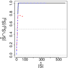
(a) (Aa), $\sigma=3$

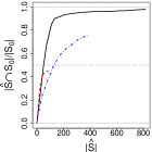
(b) (Ab), $\sigma=3$

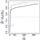
(c) (Ac), $\sigma=3$

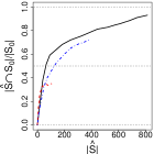
(d) (Ad), $\sigma=3$

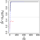
(e) (Aa), $\sigma=12$

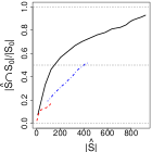
(f) (Ab), $\sigma=12$

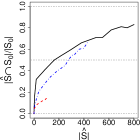
(g) (Ac), $\sigma=12$

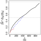
(h) (Ad), $\sigma=12$

Figure 3: Plot of $\frac{|\hat{S}\cap S_{0}|}{|\hat{S}|}$ versus $|\hat{S}|$ for block diagonal model. Cluster representative Lasso (CRL, black solid line), cluster group Lasso (CGL, blue dashed-dotted line), and Lasso (red dashed line).

From Figure 3 we infer that for the block diagonal simulation model the two methods CRL and CGL outperform the Lasso concerning variable screening. Taking a closer look, the Cluster Lasso methods CRL and CGL benefit more when having a lot of active variables in a cluster as in settings (Aa) and (Ac).

5.1.2 Single block model

We simulate the covariables $X\sim\mathcal{N}_{p}(0,\Sigma_{B})$ where

$$\Sigma_{B;i,j}=\begin{cases}1,&i=j,\\ 0.9,&i,j\in\{1,\dots,30\}\ \text{and}\ i\neq j,\\ 0,&\text{else}.\end{cases}$$

Such a $\Sigma_{B}$ corresponds to a single group of strongly correlated variables of size 30. The rest of the 970 variables are uncorrelated. For the regression parameter $\beta^{0}$ we consider the following configurations:

• $S_{0}=\{1,2,\ldots,15\}\cup\{31,32,\ldots,35\}$ and for any $j\in S_{0}$ we sample $\beta^{0}_{j}$ from the set $\{2/s_{0},4/s_{0},\ldots,2\}$ without replacement (anew in each simulation run).

• $S_{0}=\{1,2,\ldots,5\}\cup\{31,32,\ldots,45\}$ and for any $j\in S_{0}$ we sample $\beta^{0}_{j}$ from the set $\{2/s_{0},4/s_{0},\ldots,2\}$ without replacement (anew in each simulation run).

• $\beta^{0}$ as in (Ba) but we switch the sign of half and randomly chosen active parameters (anew in each simulation run).

• $\beta^{0}$ as in (Bb) but we switch the sign of half and randomly chosen active parameters (anew in each simulation run).

In the fist set-up (Ba), a major fraction of the active variables are in the same block of highly correlated variables. In the second scenario (Bb), most of the active variables are distributed among the independent variables. The remaining two configurations (Bc) and (Bd) are modifications in terms of random sign changes. The results are described in Table 3 and Figure 4.

$\sigma$	Method	(Ba)	(Bb)	(Bc)	(Bd)
	CRL	16.73 (2.55)	27.91 (4.80)	15.49 (2.93)	22.17 (4.47)
3	CGL	247.52 (28.74)	54.73 (10.59)	21.37 (9.51)	31.58 (14.17)
	Lasso	17.13 (3.01)	27.18 (4.51)	15.02 (2.74)	21.91 (4.48)
	CRL	173.89 (23.69)	181.62 (24.24)	161.01 (23.19)	175.49 (23.61)
12	CGL	384.78 (48.26)	191.26 (25.55)	159.40 (23.88)	174.49 (25.40)
	Lasso	173.37 (23.23)	178.86 (23.80)	160.55 (22.80)	174.14 (23.14)

Table 3: MSE for the single block model with standard deviations in brackets.

In Table 3 we see that over all the configurations the CRL method performs as well as the Lasso, and both of them outperform the CGL. We again find that the CGL method gains in predictive performance when the signs of the coefficient vector are not the same everywhere, and this benefit is more pronounced when compared to the the block diagonal model.

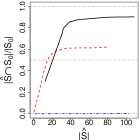
(a) (Ba), $\sigma=3$

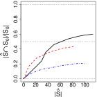
(b) (Bb), $\sigma=3$

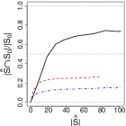
(c) (Bc), $\sigma=3$

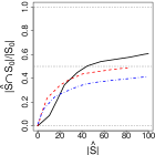
(d) (Bd), $\sigma=3$

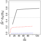
(e) (Ba), $\sigma=12$

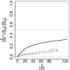
(f) (Bb), $\sigma=12$

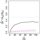
(g) (Bc), $\sigma=12$

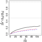
(h) (Bd), $\sigma=12$

Figure 4: Plot of $\frac{|\hat{S}\cap S_{0}|}{|\hat{S}|}$ versus $|\hat{S}|$ for single block model. Cluster representative Lasso (CRL, black solid line), cluster group Lasso (CGL, blue dashed-dotted line), and Lasso (red dashed line).

The plots in Figure 4 for variable screening show that the CRL method performs better than the Lasso for all of the configurations. The CGL method is clearly inferior to the Lasso especially in the setting (Ba) where the CGL seems to have severe problems in finding the true active variables.

5.1.3 Duo block model

We simulate the covariables $X$ according to $\mathcal{N}_{p}(0,\Sigma_{C})$ where $\Sigma_{C}$ is a block diagonal matrix. We use the $2\times 2$ block matrices

$$\Gamma=\begin{bmatrix}1&0.9\\ 0.9&1\end{bmatrix},$$

and the block diagonal of $\Sigma_{C}$ consists now of 500 such block matrices $\Gamma$. In this setting we only look at one set-up for the parameter $\beta^{0}$:

• $S_{0}=\{1,\ldots,20\}$ with $\beta^{0}_{j}=\begin{cases}2,&j\in\{1,3,5,7,9,11,13,15,17,19\},\\ \frac{\frac{1}{3}\sqrt{\frac{\log{p}}{n}}\sigma}{1.9},&j\in\{2,4,6,8,10,12,14,16,18,20\}.\end{cases}$

The idea of choosing the parameters in this way is given by the fact that the Lasso would typically not select the variables from $\{2,4,6,\ldots,20\}$ but selecting the other from $\{1,3,5,\ldots,19\}$. The following Table 4 and Figure 5 show the simulation results for the duo block model.

$\sigma$	Method	(C)
	CRL	22.45 (4.26)
3	CGL	32.00 (6.50)
	Lasso	22.45 (4.64)
	CRL	190.93 (25.45)
12	CGL	193.97 (27.05)
	Lasso	190.91 (25.64)

Table 4: MSE for duo block model with standard deviations in brackets.

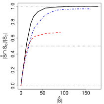
(a) (C), $\sigma=3$

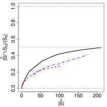
(b) (C), $\sigma=12$

Figure 5: Plot of $\frac{|\hat{S}\cap S_{0}|}{|\hat{S}|}$ versus $|\hat{S}|$ for duo block model. Cluster representative Lasso (CRL, black solid line), cluster group Lasso (CGL, blue dashed-dotted line), and Lasso (red dashed line).

From Table 4 we infer that for the duo block model, all three estimation methods have a similar prediction performance. Especially for $\sigma=12$ we see no difference between the methods. But in terms of variable screening, we see in Figure 5 that the two techniques CRL and CGL are clearly better than the Lasso.

5.2 Pseudo-real data

For the pseudo real data example described below, we also consider the CRL method with ordinary hierarchical clustering as detailed in Section 2.2. We denote the method by CRLcor.

We consider here an example with real data design matrix ${\bf X}$ but synthetic regression coefficients $\beta^{0}$ and simulated Gaussian errors ${\cal N}_{n}(0,\sigma^{2}I)$ in a linear model as in (1). For the real data design matrix ${\bf X}$ we consider a data set about riboflavin (vitamin B2) production by bacillus subtilis. That data has been provided by DSM (Switzerland). The covariates are measurements of the logarithmic expression level of $4088$ genes (and the response variable ${\bf Y}$ is the logarithm of the riboflavin production rate, but we do not use it here). The data consists of $n=71$ samples of genetically engineered mutants of bacillus subtilis. There are different strains of bacillus subtilis which are cultured under different fermentation conditions, which makes the population rather heterogeneous.

We reduce the dimension to $p=1000$ covariates which have largest empirical variances and choose the size of the active set as $s_{0}=10$.

• $S_{0}$ is chosen as a randomly selected variable $k$ and the nine covariates which have highest absolute correlation to variable $k$ (anew in each simulation run). For each $j\in S_{0}$ we use $\beta^{0}_{j}=1$.

• $S_{0}$ is chosen as one randomly selected entry in each of the five biggest clusters of both clustering methods (using either Algorithm 1 or hierarchical clustering as described in Section 2.2) resulting in $s_{0}=10$ (anew in each simulation run). For each $j\in S_{0}$ we use $\beta^{0}_{j}=1$.

The results are given in Table 5 and Figure 6, based on 50 independent simulation runs.

$\sigma$	Method	(D1)	(D2)
	CRL	2.47 (0.94)	2.99 (0.72)
3	CGL	2.36 (0.93)	3.13 (0.74)
	Lasso	2.47 (0.94)	2.96 (0.60)
	CRLcor	39.02 (25.15)	7.08 (2.76)
	CRL	19.62 (10.11)	14.80 (4.91)
12	CGL	17.49 (9.28)	14.90 (5.44)
	Lasso	19.63 (10.00)	15.66 (4.84)
	CRLcor	50.40 (27.68)	15.46 (5.74)

Table 5: Prediction error for the pseudo real riboflavin data with standard deviations in brackets.

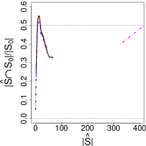
(a) (D1), $\sigma=3$

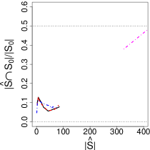
(b) (D1), $\sigma=12$

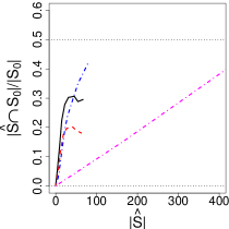
(c) (D2), $\sigma=3$

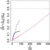
(d) (D2), $\sigma=12$

Figure 6: Plots of $\frac{|\hat{S}\cap S_{0}|}{|S_{0}|}$ versus $|\hat{S}|$ for the pseudo real riboflavin data. Cluster representative Lasso (CRL, black solid line), cluster group Lasso (CGL, blue dashed-dotted line), Lasso (red dashed line) and CRLcor (magenta dashed-dotted line).

Table 5 shows that we do not really gain any predictive power when using the proposed cluster lasso methods CRL or CGL: this finding is consistent with the reported results for simulated data in Section 5.1. The method CRLcor, using standard hierarchical clustering based on correlations (see Section 2.2) performs very poorly: the reason is that the automatically chosen number of clusters results in a partition with one very large cluster, and the representative mean value of such a very large cluster seems to be inappropriate. Using the group Lasso for such a partition (i.e., clustering) is ill-posed as well since the group size of such a large cluster is larger than sample size $n$.

Figure 6 shows a somewhat different picture for variable screening. For the setting (D1), all methods except CRLcor perform similarly, but for (D2), the two cluster Lasso methods CRL and CGL perform better than plain Lasso. Especially for the low noise level $\sigma=3$ case, we see a substantial performance gain of the CRL and CGL compared to the Lasso. Nevertheless, the improvement over plain Lasso is less pronounced than for quite a few of the simulated models in Section 5.1. The CRLcor method is again performing very poorly: the reason is the same as mentioned above for prediction while in addition, if the large cluster is selected, it results in a large contribution of the cardinality $|\hat{S}|$.

5.3 Summarizing the empirical results

We clearly see that in the pseudo real data example and most of the simulation settings, the cluster Lasso techniques (CRL and CGL) outperform the Lasso in terms of variable screening; the gain is less pronounced for the pseudo real data example. Considering prediction, the CRL and the Lasso display similar performance while the CGL is not keeping up with them. Such a deficit of the CGL method seems to be caused for cases where we have many non-active variables in an active group, leading to an efficiency loss: it might be repaired by using a sparse group Lasso (Friedman et al., 2010a, ). The difference between the clustering methods, Algorithm 1 and standard hierarchical clustering based on correlations (see Section 2.2), is essentially nonexistent for the simulation models in Section 5.1 while for the pseudo real data example in Section 5.2, the disagreement is huge and our novel Algorithm 1 leads to much better results.

6 Conclusions

We consider estimation in a high-dimensional linear model with strongly correlated variables. In such a setting, single variables cannot (or are at least very difficult to) be identified. We propose to group or cluster the variables first and do subsequent estimation with the Lasso for cluster-representatives (CRL: cluster representative Lasso) or with the group Lasso using the structure of the inferred clusters (CGL: Cluster group Lasso). Regarding the first step, we present a new bottom-up agglomerative clustering algorithm which aims for small canonical correlations between groups: we prove that it finds an optimal solution, that it is statistically consistent, and we give a simple rule for selecting the number of clusters. This new algorithm is motivated by the natural idea to address the problem of almost linear dependence between variables, but if preferred, it can be replaced by another suitable clustering procedure.

We present some theory which: (i) shows that canonical correlation based clustering leads to a (much) improved compatibility constant for the cluster group Lasso; and (ii) addresses bias and detection issues when doing subsequent estimation on cluster representatives, e.g. as with the CRL method. Regarding the second issue (ii), one favorable scenario is for (nearly) uncorrelated clusters with potentially many active variables in a cluster: the bias due to working with cluster representatives is small if the within group correlation is high, and detection is good if the regression coefficients within a group do not cancel. The other beneficial setting is for clusters with at most one active variable per cluster but the between cluster correlation does not need to be very small: if the cluster size is large or the correlation within the clusters is large, the bias due to cluster representatives is small and detection works well. We note that large cluster sizes cannot be properly handled by the cluster group Lasso while they can be advantageous for the cluster representative Lasso; instead of the group Lasso, one should take for such cases a sparse group Lasso (Friedman et al., 2010a, ) or a smoothed group Lasso (Meier et al.,, 2009). Our theoretical analysis sheds light when and why estimation with cluster representatives works well and leads to improvements, in comparison to the plain Lasso.

We complement the theoretical analysis with various empirical results which confirm that the cluster Lasso methods (CRL and CGL) are particularly attractive for improved variable screening in comparison to the plain Lasso. In view of the fact that variable screening and dimension reduction (in terms of the original variables) is one of the main applications of Lasso in high-dimensional data analysis, the cluster Lasso methods are an attractive and often better alternative for this task.

7 Proofs

7.1 Proof of Theorem 2.1

We first show an obvious result.

Lemma 7.1

Consider a partition ${\cal G}=\{G_{1},\ldots,G_{q}\}$ which satisfies (2). Then, for every $r,\ell\in\{1,\ldots,q\}$ with $r\neq\ell$:

$$\hat{\rho}_{\mathrm{can}}(J_{1},J_{2})\leq\tau\ \mbox{for all subsets}\ J_{1}\subseteq G_{r},\ J_{2}\subseteq G_{\ell}.$$

The proof follows immediately from the inequality

$$\hat{\rho}_{\mathrm{can}}(J_{1},J_{2})\leq\hat{\rho}_{\mathrm{can}}(G_{r},G_{\ell}).$$

$\Box$

For proving Theorem 2.1, the fact that we obtain a solution satisfying (2) is a straightforward consequence of the definition of the algorithm which continues to merge groups until all canonical correlations between groups are less or equal to $\tau$.

We now prove that the obtained partition is the finest clustering with $\tau$-separation. Let $\hat{\cal G}(\tau)=\{G_{1},\ldots,G_{q}\}$ be an arbitrary clustering with $\tau$-separation and $\hat{\cal G}_{b},b=1,\ldots,b^{*}$, be the sequence of partitions generated by the algorithm (where $b^{*}$ is the stopping (first) iteration where $\tau$-separation is reached). We need to show that $\hat{\cal G}_{b^{*}}$ is a finer partition of $\{1,\ldots,p\}$ than $\hat{\cal G}(\tau)$. Here, the meaning of “finer than” is not strict, i.e., including “equal to”. To this end, it suffices to prove by induction that $\hat{\cal G}_{b}$ is finer than $\hat{\cal G}(\tau)$ for $b=1,\ldots,b^{*}$. This is certainly true for $b=1$ since the algorithm begins with the finest partition of $\{1,\ldots,p\}$. Now assume the induction condition that $\hat{\cal G}_{b}$ is finer than $\hat{\cal G}(\tau)$ for $b<b^{*}$. The algorithm computes $\hat{\cal G}_{b+1}$ by merging two members, say $G^{\prime}$ and $G^{\prime\prime}$, of ${\cal G}_{b}$ such that $\hat{\rho}_{\mathrm{can}}(G^{\prime},G^{\prime\prime})>\tau$. Since $\hat{\cal G}_{b}$ is finer than $\hat{\cal G}(\tau)$, there must exist members $G_{j_{1}}$ and $G_{j_{2}}$ of $\hat{\cal G}(\tau)$ such that $G^{\prime}\subseteq G_{j_{1}}$ and $G^{\prime\prime}\subseteq G_{j_{2}}$. This implies $\hat{\rho}_{\mathrm{can}}(G_{j_{1}},G_{j_{2}})\geq\hat{\rho}_{\mathrm{can}}(G^{\prime},G^{\prime\prime})>\tau$, see Lemma 7.1. Since $\hat{\rho}_{\mathrm{can}}(G_{j},G_{k})\leq\tau$ for all $j\neq k$, we must have $j_{1}=j_{2}$. Thus, the algorithm merges two subsets of a common member (namely $G_{j_{1}}=G_{j_{2}}$) of $\hat{\cal G}(\tau)$. It follows that $\hat{\cal G}_{b+1}$ is still finer than $\hat{\cal G}(\tau)$. $\Box$

7.2 Proof of Theorem 2.2

For ease of notation, we abbreviate a group index $G_{r}$ by $r$. The proof of Theorem 2.2 is based on the following bound for the maximum difference between the sample and population correlations of linear combination of variables. Define

$$\Delta_{r,{\ell}}=\max_{u\neq 0,v\neq 0}\big{|}\hat{\rho}({\bf X}^{(r)}u,{\bf X}^{(\ell)}v)-\rho(u^{T}X^{(r)},v^{T}X^{(\ell)})\big{|}.$$

Lemma 7.2

Consider ${\bf X}$ as in (3) and ${\cal G}^{0}=\{G_{1},\ldots,G_{q}\}$ a partition of $\{1,\ldots,p\}$. Let $\Sigma_{r,{\ell}}=\mathrm{Cov}(X^{(r)},X^{(\ell)})$, $t>0$ and $d_{r}=\mathrm{rank}(\Sigma_{r,r})$. Define $\Delta^{*}_{r,{\ell}}$ by (4). Then,

$$\mathbb{P}[\max_{1\leq j<k\leq q}(\Delta_{r,{\ell}}-\Delta^{*}_{r,{\ell}})\geq 0]\leq\exp(-t).$$

Proof of Lemma 7.2. Taking a new coordinate system if necessary, we may assume without loss of generality that $\Sigma_{r,r}=I_{d_{r}}$ and $\Sigma_{{\ell},{\ell}}=I_{d_{\ell}}$. Let $\hat{\Sigma}_{r,{\ell}}$ be the sample versions of $\Sigma_{r,{\ell}}$. For $r\neq\ell$, we write a linear regression model ${\bf X}^{(\ell)}={\bf X}^{(r)}\Sigma_{r,{\ell}}+{\boldsymbol{\varepsilon}}^{(r,{\ell})}V_{r,{\ell}}^{1/2}$ such that ${\boldsymbol{\varepsilon}}^{(r,{\ell})}$ is an $n\times d_{\ell}$ matrix of i.i.d. $N(0,1)$ entries independent of ${\bf X}^{(r)}$ and $\|V_{r,{\ell}}^{1/2}\|_{(S)}\leq 1$, where $\|\cdot\|_{(S)}$ is the spectrum norm. This gives $\hat{\Sigma}_{r,{\ell}}=\hat{\Sigma}_{r,r}\Sigma_{r,{\ell}}+({\bf X}^{(r)})^{T}{\boldsymbol{\varepsilon}}^{(r,{\ell})}V_{r,{\ell}}^{1/2}/n$. Let $U_{r}U_{r}^{T}$ be the SVD of the projection ${\bf X}^{(r)}\hat{\Sigma}_{r,r}^{-1}({\bf X}^{(r)})^{T}/n$, with $U_{r}\in\mathbb{R}^{n\times d_{r}}$. Since ${\bf X}^{(r)}$ is independent of ${\boldsymbol{\varepsilon}}^{(r,{\ell})}$, $U_{r}^{T}{\boldsymbol{\varepsilon}}^{(r,{\ell})}$ is a $d_{r}\times d_{\ell}$ matrix of i.i.d. $N(0,1)$ entries. Let

$$\Omega_{r}=\big{\{}\|\hat{\Sigma}_{r,r}^{1/2}-I_{d_{r}}\|_{(S)}\leq t_{r}\},\ \Omega_{r,{\ell}}=\big{\{}\|U_{r}^{T}{\boldsymbol{\varepsilon}}^{(r,{\ell})}/\sqrt{n}\|_{(S)}\leq t_{r}\wedge t_{\ell}\big{\}}.$$

It follows from (4) and Theorem II.13 of Davidson and Szarek, (2001) that

$$\max\big{\{}\mathbb{P}[\Omega_{r}^{c}],\mathbb{P}[\Omega_{r,{\ell}}^{c}]\big{\}}\leq 2\mathbb{P}[N(0,1)>\sqrt{2(t+\log(q(q+1)))}]\leq 2e^{-t}/\{q(q+1)\}.$$

In the event $\Omega_{r}$, we have

$$\Delta_{r,r} = \max_{\|u\|_{2}=\|v\|_{2}=1}\Big{|}\frac{u\hat{\Sigma}_{r,r}v}{\|\hat{\Sigma}_{r,r}^{1/2}u\|_{2}\|\hat{\Sigma}_{r,r}^{1/2}v\|_{2}}-u^{T}v\Big{|}$$

$$\leq \|\hat{\Sigma}_{r,r}-I_{d_{r}}\|_{(S)}/(1-t_{r})^{2}+\max_{\|u\|_{2}=\|v\|_{2}=1}\Big{|}\frac{u^{T}v}{\|\hat{\Sigma}_{r,r}^{1/2}u\|_{2}\|\hat{\Sigma}_{r,r}^{1/2}v\|_{2}}-u^{T}v\Big{|}$$

$$\leq \{(1+t_{r})^{2}-1\}/(1-t_{r})^{2}+1/(1-t_{r})^{2}-1$$

$$= \Delta^{*}_{r,r}.$$

For $r\neq\ell$, the variable change $u\to\hat{\Sigma}_{r,r}^{-1/2}u$ gives

$$\Delta_{r,{\ell}}=\max_{\|u\|_{2}=\|v\|_{2}=1}\Big{|}u^{T}\hat{\Sigma}_{r,r}^{-1/2}\Big{(}\frac{\hat{\Sigma}_{r,{\ell}}}{\|\hat{\Sigma}_{\ell,\ell}^{1/2}v\|_{2}}-\frac{\Sigma_{r,{\ell}}}{\|\hat{\Sigma}_{r,r}^{-1/2}u\|_{2}}\Big{)}v\Big{|}.$$

In the event $\Omega_{r}\cap\Omega_{\ell}\cap\Omega_{r,{\ell}}$, we have

$$\Delta_{r,{\ell}} \leq \max_{\|u\|_{2}=\|v\|_{2}=1}\Big{\{}\big{|}u\hat{\Sigma}_{r,r}^{-1/2}(\hat{\Sigma}_{r,{\ell}}-\Sigma_{r,{\ell}})v\big{|}/\|\hat{\Sigma}_{\ell,\ell}^{1/2}v\|_{2}$$

$$\qquad+\Big{|}u^{T}\hat{\Sigma}_{r,r}^{-1/2}\Sigma_{r,{\ell}}v(1/\|\hat{\Sigma}_{\ell,\ell}^{1/2}v\|_{2}-1/\|\hat{\Sigma}_{r,r}^{-1/2}u\|_{2})\Big{|}\Big{\}}$$

$$\leq \max_{\|u\|_{2}=\|v\|_{2}=1}\Big{\{}\|\hat{\Sigma}_{r,r}^{-1/2}(\hat{\Sigma}_{r,{\ell}}-\Sigma_{r,{\ell}})\big{\|}_{(S)}/\|\hat{\Sigma}_{\ell,\ell}^{1/2}v\|_{2}+\Big{|}\|\hat{\Sigma}_{r,r}^{-1/2}u\|_{2}/\|\hat{\Sigma}_{\ell,\ell}^{1/2}v\|_{2}-1\Big{|}\Big{\}}$$

$$\leq \|(\hat{\Sigma}_{r,r}^{1/2}-\hat{\Sigma}_{r,r}^{-1/2})\Sigma_{r,{\ell}}+\hat{\Sigma}_{r,r}^{-1/2}({\bf X}^{(r)})^{T}{\boldsymbol{\varepsilon}}^{(r,{\ell})}V_{r,{\ell}}^{1/2}/n\|_{(S)}/(1-t_{\ell})$$

$$+1/\{(1-t_{r})(1-t_{\ell})\}-1$$

$$\leq \big{(}\|\hat{\Sigma}_{r,r}^{1/2}-\hat{\Sigma}_{r,r}^{-1/2}\|_{(S)}+\|U_{r}^{T}{\boldsymbol{\varepsilon}}^{(r,{\ell})}/\sqrt{n}\|_{(S)}\big{)}/(1-t_{\ell})+(t_{r}+t_{\ell})/\{(1-t_{r})(1-t_{\ell})\}$$

$$\leq \{1/(1-t_{r})-(1-t_{r})+t_{r}\wedge t_{\ell}\}/(1-t_{\ell})+(t_{r}+t_{\ell})/\{(1-t_{r})(1-t_{\ell})\}$$

$$= (1-(1-t_{r})^{2}+(1-t_{r})(t_{r}\wedge t_{\ell})+t_{r}+t_{\ell})/\{(1-t_{r})(1-t_{\ell})\}.$$

Thus, for $t_{r}\leq t_{\ell}$, we find $\Delta_{r,{\ell}}\leq\Delta^{*}_{r,{\ell}}$. Since $\Delta_{r,{\ell}}=\Delta_{\ell,r}$, the above bounds hold simultaneously in the intersection of all $\Omega_{r}$ and those $\Omega_{r,{\ell}}$ with either $t_{r}<t_{\ell}$ or $r<\ell$ for $t_{r}=t_{\ell}$. Since there are totally $q+q(q-1)/2=q(q+1)/2$ such events, $\mathbb{P}[\Delta_{r,{\ell}}\leq\Delta^{*}_{r,{\ell}}\ \forall r,{\ell}]\geq 1-\exp(-t)$. $\hfill\Box$

Proof of Theorem 2.2. It follows from (5) that ${\cal G}^{0}$ is the finest population clustering with $\tau$-separation for all $\tau_{-}\leq\tau\leq\tau_{+}$. Since $\rho_{can}(G_{r},G_{\ell})=\max_{u,v}\rho(u^{T}X^{(r)},v^{T}X^{(\ell)})$ and $\hat{\rho}_{can}(G_{r},G_{\ell})=\max_{u,v}\hat{\rho}({\bf X}^{(r)}u,{\bf X}^{(\ell)}v)$, (5) and Lemma 7.2 implies that with at least probability $1-e^{-t}$, the inequalities

$$\hat{\rho}_{can}(G_{r},G_{\ell})\leq\rho_{can}(G_{r},G_{\ell})+\Delta^{*}_{r,{\ell}}\leq\tau_{-},$$

$$\max_{k_{1}<k_{2}}\hat{\rho}_{can}(G_{r;k_{1}},G_{r;k_{2}})\geq\max_{k_{1}<k_{2}}\rho_{can}(G_{r;k_{1}},G_{r;k_{2}})-\Delta^{*}_{r,r}\geq\tau_{+},$$

hold simultaneously for all $r<\ell$ and nontrivial partitions $\{G_{r;k},k\leq q_{r}\}$ of $G_{r},r=1,\ldots,q$. In this case, ${\cal G}^{0}$ is also the finest sample clustering with $\tau$-separation for all $\tau_{-}\leq\tau\leq\tau_{+}$. The conclusion follows from Theorem 2.1. $\Box$

7.3 Proof of Theorem 4.1

We write for notational simplicity $S_{0}:=S_{0,{\rm Group}}$ and $s_{0}:=|S_{0,{\rm Group}}|$. Note first that for all $r$,

$$\|{\bf X}^{(G_{r})}\beta_{G_{r}}\|_{2}^{2}=n\beta_{G_{r}}^{T}\hat{\Sigma}_{r,r}\beta_{G_{r}}=n\|\gamma_{G_{r}}\|_{2}^{2},$$

where $\gamma_{G_{r}}:=\Sigma_{r,r}^{1/2}\beta_{G_{r}}$. Moreover,

$$\|{\bf X}^{(S_{0})}\beta_{S_{0}}\|_{2}^{2}=n\gamma_{S_{0}}^{T}\hat{R}_{S_{0}}\gamma_{S_{0}}.$$

It follows that

$$\sum_{r\in S_{0}}\|{\bf X}^{(G_{r})}\beta_{G_{r}}\|_{2}^{2}=n\|\gamma_{S_{0}}\|_{2}^{2}$$

$$\leq n\gamma_{S_{0}}^{T}\hat{R}_{S_{0}}\gamma_{S_{0}}/\hat{\Lambda}_{\rm min}^{2}=\|X^{(S_{0})}\beta_{S_{0}}\|_{2}^{2}/\hat{\Lambda}_{\rm min}^{2}.$$ (32)

Furthermore,

$$\biggl{|}\beta_{S_{0}}^{T}({\bf X}^{(S_{0})})^{T}{\bf X}^{(S_{0}^{c})}\beta_{S_{0}^{c}}\biggr{|}=n\biggl{|}\sum_{r\in S_{0}}\sum_{\ell\in S_{0}^{c}}\beta_{G_{r}}^{T}\hat{\Sigma}_{r,\ell}\beta_{G_{\ell}}^{T}\biggr{|}$$

$$=n\biggl{|}\sum_{r\in S_{0}}\sum_{\ell\in S_{0}^{c}}\gamma_{G_{r}}^{T}\hat{\Sigma}_{r,r}^{-1/2}\hat{\Sigma}_{r,\ell}\hat{\Sigma}_{\ell,\ell}^{-1/2}\gamma_{G_{\ell}}\biggr{|}\leq n\sum_{r\in S_{0}}\sum_{\ell\in S_{0}^{c}}\hat{\rho}_{\rm can}(G_{r},G_{\ell})\|\gamma_{G_{r}}\|_{2}\|\gamma_{G_{\ell}}\|_{2}$$

$$=\sum_{r\in S_{0}}\sum_{\ell\in S_{0}^{c}}\hat{\rho}_{\rm can}(G_{r},G_{\ell})\|{\bf X}^{(G_{r})}\beta_{G_{r}}\|_{2}\|{\bf X}^{(G_{\ell})}\beta_{G_{\ell}}\|_{2}$$

$$=\sum_{r\in S_{0}}\sum_{\ell\in S_{0}^{c}}{\hat{\rho}_{\rm can}(G_{r},G_{\ell})}{\bar{m}\over\sqrt{m_{r}m_{\ell}}}\|{\bf X}^{(G_{r})}\beta_{G_{r}}\|_{2}\sqrt{m_{r}\over\bar{m}}\|{\bf X}^{(G_{\ell})}\beta_{G_{\ell}}\|_{2}\sqrt{m_{\ell}\over\bar{m}}$$

$$\leq\rho\|{\bf X}^{(S_{0})}\beta_{S_{0}}\|_{2,1}\|{\bf X}^{(S_{0}^{c})}\beta_{S_{0}^{c}}\|_{2,1}.$$

Hence, for all $\beta$ satisfying $\|\beta_{S_{0}^{c}}\|_{2,1}\leq 3\|\beta_{S_{0}}\|_{2,1}$, we have

$$\biggl{|}\beta_{S_{0}}^{T}({\bf X}^{(S_{0})})^{T}{\bf X}^{(S_{0}^{c})}\beta_{S_{0}^{c}}\biggr{|}\leq 3\rho\|\beta_{S_{0}}\|_{2,1}^{2}.$$ (33)

Applying the Cauchy-Schwarz inequality and (7.3) gives

$$\|\beta_{S_{0}}\|_{2,1}^{2}:=\biggl{(}\sum_{r\in S_{0}}\|{\bf X}^{(G_{r})}\beta_{G_{r}}\|_{2}\sqrt{m_{r}/\bar{m}}\biggr{)}^{2}$$

$$\leq{\sum_{r\in S_{0}}m_{r}\over\bar{m}}\sum_{r\in S_{0}}\|{\bf X}^{(G_{r})}\beta_{G_{r}}\|_{2}^{2}\leq{\sum_{r\in S_{0}}m_{r}\over\bar{m}}{\|{\bf X}^{(S_{0})}\beta_{S_{0}}\|_{2}^{2}\over\hat{\Lambda}_{\rm min}^{2}}={s_{0}\bar{m}_{S_{0}}\over\bar{m}}{\|{\bf X}^{(S_{0})}\beta_{S_{0}}\|_{2}^{2}\over\hat{\Lambda}_{\rm min}^{2}}.$$

Insert this in (33) to get

$$\biggl{|}\beta_{S_{0}}^{T}({\bf X}^{(S_{0})})^{T}{\bf X}^{(S_{0}^{c})}\beta_{S_{0}^{c}}\biggr{|}\leq\rho{3s_{0}\bar{m}_{S_{0}}\over\bar{m}\hat{\Lambda}_{\rm min}^{2}}\|{\bf X}^{(S_{0})}\beta_{S_{0}}\|_{2}^{2}.$$

Use the assumption that

$$\rho{3s_{0}\bar{m}_{S_{0}}\over\bar{m}\hat{\Lambda}_{\rm min}^{2}}<1,$$

and apply Lemma 6.26 in Bühlmann and van de Geer, (2011) to conclude that

$$\|{\bf X}^{(S_{0})}\beta_{S_{0}}\|_{2}^{2}\leq\biggl{(}1-\rho{3s_{0}\bar{m}_{S_{0}}\over\bar{m}\hat{\Lambda}_{\rm min}^{2}}\biggr{)}^{-2}\|{\bf X}\beta\|_{2}^{2}.$$

Hence,

$$\|\beta_{S_{0}}\|_{2,1}^{2}\leq{s_{0}\bar{m}_{S_{0}}\over\bar{m}}{\|{\bf X}^{(S_{0})}\beta_{S_{0}}\|_{2}^{2}\over\hat{\Lambda}_{\rm min}^{2}}$$

$$\leq\biggl{(}1-\rho{3s_{0}\bar{m}_{S_{0}}\over\bar{m}\hat{\Lambda}_{\rm min}^{2}}\biggr{)}^{-2}\biggl{(}{s_{0}\bar{m}_{S_{0}}\over\bar{m}}\biggr{)}{\|{\bf X}\beta\|_{2}^{2}\over\hat{\Lambda}_{\rm min}^{2}}.$$

This leads to the first lower bound in the statement of the theorem. The second lower bound follows immediately by the incoherence assumption for $\rho$. Furthermore, it is not difficult to see that $\hat{\Lambda}_{\rm min}^{2}\geq(1-|S_{0,{\rm Group}}|\rho_{S_{0,{\rm Group}}})$, and using the incoherence assumption for $\rho_{S_{0,{\rm Group}}}$ leads to strict positivity. $\Box$

7.4 Proof of Proposition 4.2

We can invoke the analysis given in Bühlmann and van de Geer, (2011, Th.6.1). The slight deviations involve: (i) use that $\mathbb{E}[\eta_{i}|{\bf Z}]=0$; (ii): due to the Gaussian assumption $\mathrm{Var}(\eta_{i}|{\bf Z})$ is constant equaling $\mathrm{Var}(\eta_{i}|{\bf Z})=\mathbb{E}[\mathrm{Var}(\eta_{i}|{\bf Z})]=\mathrm{Var}(\eta_{i})=\xi^{2}=\sigma^{2}+\mathbb{E}[(\mu_{X}-\mu_{Z})^{2}]$; and (iii): the probability bound in Bühlmann and van de Geer, (2011, Lem.6.2) can be easily obtained for non-standardized variables when multiplying $\lambda_{0}$ with $\|\hat{\sigma}_{{\bf Z}}\|_{\infty}$. The issues (ii) and (iii) explain the factors appearing in the definition of $\lambda_{0}$. $\Box$

7.5 Proof of Proposition 4.3

Because of uncorrelatedness of $\bar{X}^{(r)}$ among $r=1,\ldots,q$, we have:

$$\gamma^{0}_{r} = \frac{\mathrm{Cov}(Y,\bar{X}^{(r)})}{\mathrm{Var}(\bar{X}^{(r)})}=|G_{r}|^{-1}\frac{\sum_{j\in G_{r}}\mathrm{Cov}(Y,X^{(j)})}{\mathrm{Var}(\bar{X}^{(r)})}$$

$$= |G_{r}|\frac{\sum_{j\in G_{r}}\beta_{j}^{0}\mathrm{Var}(X^{(j)})+\sum_{i\neq j}\beta^{0}_{i}\mathrm{Cov}(X^{(i)},X^{(j)})}{\sum_{\ell\in G_{r}}(\mathrm{Var}(X^{(\ell)})+\sum_{i\neq\ell}\mathrm{Cov}(X^{(i)},X^{(\ell)}))}.$$

Define

$$w_{j}=\frac{\mathrm{Var}(X^{(j)})+\sum_{i\neq j}\mathrm{Cov}(X^{(i)},X^{(j)})}{\sum_{\ell\in G_{r}}(\mathrm{Var}(X^{(\ell)})+\sum_{i\neq\ell}\mathrm{Cov}(X^{(i)},X^{(\ell)}))}.$$ (34)

Then, $\sum_{j\in G_{r}}w_{j}=1$ and $\gamma^{0}_{r}=\sum_{j\in G_{r}}w_{j}\beta^{0}_{j}$.

The statement 1 follows immediately from (34). Regarding statement 2, we read off from (34) that $w_{j}\equiv|G_{r}|^{-1}$ for all $j\in G_{r}$ and hence $\gamma^{0}_{r}=\sum_{j\in G_{r}}\beta_{j}^{0}$. $\Box$

7.6 Proof of Proposition 4.4

We have

$$\gamma^{0}_{r}=\frac{\mathrm{Cov}(Y,\bar{X}^{(r)}|\{\bar{X}^{(\ell)};\ \ell\neq r\})}{\mathrm{Var}(\bar{X}^{(r)}|\{\bar{X}^{(\ell)};\ \ell\neq r\})},$$

since for Gaussian distributions, partial covariances equal conditional covariances (Baba et al.,, 2004, cf.). For the numerator, we have:

$$\mathrm{Cov}(Y,\bar{X}^{(r)}|\{\bar{X}^{(\ell)};\ \ell\neq r\})=|G_{r}|^{-1}\sum_{j\in G_{r}}\mathrm{Cov}(Y,X^{(j)}|\{\bar{X}^{(\ell)};\ \ell\neq r\})$$

$$= |G_{r}|^{-1}\sum_{i,j\in G_{r}}\beta^{0}_{i}\mathrm{Cov}(X^{(i)},X^{(j)}|\{\bar{X}^{(\ell)};\ \ell\neq r\})$$

$$+ |G_{r}|^{-1}\sum_{j\in G_{r}}\sum_{i\notin G_{r}}\beta^{0}_{i}\mathrm{Cov}(X^{(i)},X^{(j)}|\{\bar{X}^{(\ell)};\ \ell\neq r\})$$

$$= |G_{r}|^{-1}\sum_{i,j\in G_{r}}\beta^{0}_{i}\mathrm{Cov}(X^{(i)},X^{(j)}|\{\bar{X}^{(\ell)};\ \ell\neq r\})+\Gamma_{r},\ |\Gamma_{r}|\leq\|\beta^{0}\|_{1}\nu.$$

for the denominator, we have:

$$\mathrm{Var}(\bar{X}^{(r)}|\{\bar{X}^{(\ell)};\ \ell\neq r\})=|G_{r}|^{-2}\sum_{i,j\in G_{r}}\mathrm{Cov}(X^{(i)},X^{(j)}|\{\bar{X}^{(\ell)};\ \ell\neq r\}).$$

Defining

$$w_{j}=\frac{\sum_{i\in G_{r}}\mathrm{Cov}(X^{(i)},X^{(j)}|\{\bar{X}^{(\ell)};\ \ell\neq r\})}{\sum_{i,\ell\in G_{r}}\mathrm{Cov}(X^{(i)},X^{(\ell)}|\{\bar{X}^{(\ell)};\ \ell\neq r\})},$$ (35)

we obtain $\gamma^{0}_{r}=|G_{r}|\sum_{j\in G_{r}}w_{j}\beta^{0}_{j}+\Delta_{r}$ with $|\Delta_{r}\leq\|\beta^{0}\|_{1}\nu/C$. The other statement follows using (35) and as statement 1. in Proposition 4.3. $\Box$

7.7 Proof of Proposition 4.5

Write

$$Y=\bar{X}^{T}\gamma^{0}+\eta=U^{T}\tilde{\beta}^{0}+\varepsilon=\bar{X}^{T}\tilde{\beta}^{0}-W\tilde{\beta}^{0}+\varepsilon.$$

Therefore,

$$\bar{X}(\tilde{\beta}^{0}-\gamma^{0})=\eta-\varepsilon+W^{T}\tilde{\beta}^{0}.$$

Taking the squares and expectation on both sides,

$$(\tilde{\beta}^{0}-\gamma^{0})^{T}\mathrm{Cov}(\bar{X})(\tilde{\beta}^{0}-\gamma^{0})=\mathbb{E}[(\eta-\varepsilon)^{2}]+\mathbb{E}|W^{T}\tilde{\beta}^{0}|^{2}=B^{2}+\mathbb{E}|W^{T}\tilde{\beta}^{0}|^{2}\leq 2\mathbb{E}|W^{T}\tilde{\beta}^{0}|^{2},$$

where the last inequality follows from (24). Since $\mathrm{Cov}(\bar{X})=\mathrm{Cov}(U)+\mathrm{Cov}(W)$, we have that $\lambda_{\mathrm{min}}^{2}(\mathrm{Cov}(\bar{X}))\geq\lambda_{\mathrm{min}}^{2}(\mathrm{Cov}(U))$. This completes the proof. $\Box$

References

- Anderson, (1984) Anderson, T. (1984). An Introduction to Multivariate Statistical Analysis. Wiley, 2nd edition edition.
- Baba et al., (2004) Baba, K., Shibata, R., and Sibuya, M. (2004). Partial correlation and conditional correlation as measures of conditional independence. Australian & New Zealand Journal of Statistics, 46:657–664.
- Balding, (2007) Balding, D. (2007). A tutorial on statistical methods for population association studies. Nature Reviews Genetics, 7:781–791.
- Bickel et al., (2009) Bickel, P., Ritov, Y., and Tsybakov, A. (2009). Simultaneous analysis of Lasso and Dantzig selector. Annals of Statistics, 37:1705–1732.
- Bondell and Reich, (2008) Bondell, H. and Reich, B. (2008). Simultaneous regression shrinkage, variable selection and clustering of predictors with OSCAR. Biometrics, 64:115–123.
- Bühlmann and van de Geer, (2011) Bühlmann, P. and van de Geer, S. (2011). Statistics for High-Dimensional Data: Methods, Theory and Applications. Springer Verlag.
- Carlson et al., (2004) Carlson, C., Eberle, M., Rieder, M., Yi, Q., Kruglyak, L., and Nickerson, D. (2004). Selecting a maximally informative set of single-nucleotide ploymorphisms for association analyses using linkage disequilibrium. American Jounal of Human Genetics, 74:106–120.
- Davidson and Szarek, (2001) Davidson, K. and Szarek, S. (2001). Local operator theory, random matrices and Banach spaces. In Handbook in Banach Spaces, Vol. I (eds. W.B. Johnson and J. Lindenstrauss), pages 317–366. Elsevier.
- Dettling and Bühlmann, (2004) Dettling, M. and Bühlmann, P. (2004). Finding predictive gene groups from microarray data. Journal of Multivariate Analysis, 90:106–131.
- (10) Friedman, J., Hastie, T., and Tibshirani, R. (2010a). A note on the group Lasso and a sparse group Lasso. arXiv:1001.0736v1.
- (11) Friedman, J., Hastie, T., and Tibshirani, R. (2010b). Regularized paths for generalized linear models via coordinate descent. Journal of Statistical Software, 33:1–22.
- Hastie et al., (2001) Hastie, T., Tibshirani, R., Botstein, D., and Brown, P. (2001). Supervised harvesting of expression trees. Genome Biology, 2:1–12.
- Hastie et al., (2000) Hastie, T., Tibshirani, R., Eisen, M., Alizadeh, A., Levy, R., Staudt, L., Chan, W., Botstein, D., and Brown, P. (2000). ‘Gene shaving’ as a method for identifying distinct sets of genes with similar expression patterns. Genome Biology, 1:1–21.
- Huang et al., (2011) Huang, J., Ma, S., Li, H., and Zhang, C.-H. (2011). The sparse Laplacian shrinkage estimator for high-dimensional regression. Annals of Statistics, 39:2021–2046.
- Kendall, (1957) Kendall, M. (1957). A Course in Multivariate Analysis. Griffin: London.
- Meier et al., (2009) Meier, L., van de Geer, S., and Bühlmann, P. (2009). High-dimensional additive modeling. Annals of Statistics, 37:3779–3821.
- Meinshausen, (2007) Meinshausen, N. (2007). Relaxed Lasso. Computational Statistics & Data Analysis, 52:374–393.
- Meinshausen and Bühlmann, (2006) Meinshausen, N. and Bühlmann, P. (2006). High-dimensional graphs and variable selection with the Lasso. Annals of Statistics, 34:1436–1462.
- Meinshausen and Yu, (2009) Meinshausen, N. and Yu, B. (2009). Lasso-type recovery of sparse representations for high-dimensional data. Annals of Statistics, 37:246–270.
- Segal et al., (2003) Segal, M., Dahlquist, K., and Conklin, B. (2003). Regression approaches for microarray data analysis. Journal of Computational Biology, 10:961–980.
- She, (2010) She, Y. (2010). Sparse regression with exact clustering. Electronic Journal of Statistics, 4:1055–1096.
- Sun and Zhang, (2011) Sun, T. and Zhang, C.-H. (2011). Scaled sparse linear regression. arXiv:1104.4595v1.
- Tibshirani, (1996) Tibshirani, R. (1996). Regression shrinkage and selection via the Lasso. Journal of the Royal Statistical Society, Series B, 58:267–288.
- van de Geer, (2007) van de Geer, S. (2007). The deterministic Lasso. In JSM proceedings, 2007, 140. American Statistical Association.
- van de Geer and Bühlmann, (2009) van de Geer, S. and Bühlmann, P. (2009). On the conditions used to prove oracle results for the Lasso. Electronic Journal of Statistics, 3:1360–1392.
- van de Geer and Lederer, (2011) van de Geer, S. and Lederer, J. (2011). The Lasso, correlated design, and improved oracle inequalities. In: Festschrift for Jon Wellner, IMS Collections. To appear.
- Yuan and Lin, (2006) Yuan, M. and Lin, Y. (2006). Model selection and estimation in regression with grouped variables. Journal of the Royal Statistical Society, Series B, 69:49–67.
- Zhang and Huang, (2008) Zhang, C.-H. and Huang, J. (2008). The sparsity and bias of the Lasso selection in high-dimensional linear regression. Annals of Statistics, 36:1567–1594.
- Zhao and Yu, (2006) Zhao, P. and Yu, B. (2006). On model selection consistency of Lasso. Journal of Machine Learning Research, 7:2541–2563.
- Zou, (2006) Zou, H. (2006). The adaptive Lasso and its oracle properties. Journal of the American Statistical Association, 101:1418–1429.
- Zou and Hastie, (2005) Zou, H. and Hastie, T. (2005). Regularization and variable selection via the Elastic Net. Journal of the Royal Statistical Society Series B, 67:301–320.
- Zou and Li, (2008) Zou, H. and Li, R. (2008). One-step sparse estimates in nonconcave penalized likelihood models (with discussion). Annals of Statistics, 36:1509–1566.