Abstract

Using the AdS/CFT correspondence, the effect of $\alpha^{\prime}$-correction on the value of Chiral Magnetic Effect(CME) is computed by adding a number of spinning probe D7-branes in the $\alpha^{\prime}$-corrected background. We numerically show that the magnitude of CME rises in the presence of $\alpha^{\prime}$-correction for massive solutions and this increase is more sensible at higher temperatures. However, this value does not change for massless solution. Although some of the D7-brane embeddings have no CME, after applying the $\alpha^{\prime}$-correction they find a non-zero value for the CME. We also show that the effect of $\alpha^{\prime}$-correction removes the singularity from some of the D7-brane embeddings.

1 Introduction

A new phase of Quantum Chromodynamics (QCD) called Quark-Gluon plasma (QGP) is produced at Relativistic Heavy Ion Collider (RHIC) and Large Hadron Collider (LHC) by colliding two pancakes of heavy nuclei such as Gold or Lead at a relativistic speed. It was realized that the QGP is a strongly coupled perfect fluid with very low viscosity over entropy density, $\eta/s$. Therefore in order to describe it the perturbative methods are inapplicable. Different properties of the QGP such as rapid thermalization, elliptic flow, jet quenching parameter and quarkonium dissociation have been considerably studied [1, 2, 3].

One of the interesting properties of QGP is the Chiral Magnetic Effect (CME). The presence of a strong magnetic field in the very early stages of heavy ion collision and its accompanying non-trivial gluon field configurations lead to the CME, which is the generation of an electric current along the strong magnetic field [4, 5, 6, 7, 8]. In free massless QCD the CME can be described in the following way. This theory enjoys two global $U(1)$ symmetries: vector symmetry, $U(1)_{V}$, and axial symmetry, $U(1)_{A}$. If we assume that the global vector symmetry is preserved at quantum level, $U(1)_{A}$ will be anomalous. The axial charge associated to this symmetry, given by the difference between the number of fermions with left-handed and right-handed helicities, is proportional to the winding number of non-trivial gauge field provided that the left-handed and right-handed fermions are initially equal. The spin of fermions is tightly aligned along the strong magnetic field. For a non-zero winding number, in order to have a non-zero axial charge the momentum direction of some fermions depending on the sign of winding number must be altered. This phenomena leads to an electric current along the magnetic field, the CME. There are various ways to calculate this current in the literature [6, 7, 8].

Consider an effective Lagrangian which includes the original QCD Lagrangian and an extra term $\theta(t,x)\tilde{F}^{\mu\nu}F_{\mu\nu}$ where the form of the extra term is fixed by the anomaly and $\theta(t,x)$ is a non-dynamical axion field [8]. Assuming a space-independent $\theta(t,x)$, which means $\theta(x,t)\equiv\theta(t)$, the time derivative of $\theta(t)$ can be identified by $\mu_{5}$ which is the axial chemical potential [8]. Using the effective Lagrangian the value of electric current is computed by [8]

$$J=\frac{\mu_{5}}{2\pi^{2}}B~{}.$$ (1)

Since the QGP is a strongly coupled fluid, AdS/CFT correspondence seems to be a suitable framework to describe the CME [9].

The AdS/CFT correspondence [10] states that type IIB string theory on $AdS_{5}\times S^{5}$ geometry, describing the near horizon geometry of a stack of $N_{c}$ extremal D3-branes, is dual to the four-dimensional ${\cal{N}}=4$ super Yang-Milles (SYM) theory with gauge group $SU(N_{c})$. One of the most interesting properties of this correspondence is that it is a strong/weak correspondence. In particular in the large $N_{c}$ limit a strongly coupled SYM theory is dual to the type IIb supergravity which provides a useful tool to study the strongly coupled regime of the SYM theory. This correspondence also generalized to the thermal SYM. As a result a thermal SYM theory corresponds to the supergravity in an AdS-Schwarzschild background where SYM theory temperature is identified with the Hawking temperature of AdS black hole [11].

In the context of AdS/CFT correspondence matter fields in the fundamental representation can be studied by introducing space filling flavor D7-branes in the probe limit [12] which means that the number of flavor D7-branes, $N_{f}$, are very much smaller than the number of D3-branes. The open strings stretched between D3-branes and flavor D7-branes give rise to ${\mathcal{N}}=2$ hypermultiplet in the gauge theory side. Mass of the hypermultiplet is proportional to the separation of D3- and D7-branes in transverse directions. This system, D3-D7 system, is a famous candidate to describe QCD-like theories [13]. Different aspects of adding flavor D7-branes in different backgrounds have been studied in the literature. Here we are interested in introducing D7-branes in the $\alpha^{\prime}$-corrected background to study the effect of higher order correction on the CME.

The $\alpha^{\prime}$-correction has been studied in [14, 15, 16, 17, 18, 19, 20]. The main motivation to consider $\alpha^{\prime}$-correction comes from the fact that string theory contains higher derivative corrections arising from stringy effects. The leading order correction in $1/\lambda$, where $\lambda$ is the t’Hooft coupling constant in gauge theory side, arises from stringy corrections to the low energy effective action of type IIb supergravity, $\alpha^{\prime 3}{\cal{R}}^{4}$. An understanding of how these computations are affected by finite $\lambda$ correction is essential for precise theoretical predictions.

2 Review on Holographic CME

Using D3-D7 system an interesting holographic description for the CME is introduced in [21]. Our aim in this section is to give a short review on this paper. In order to do that, we consider a supersymmetric intersection of $N_{c}$ D3-branes and $N_{f}$ probe D7-branes as

$$\begin{array}[]{ccccccccccc}&0&1&2&3&4&5&6&7&8&9\\ D3&\times&\times&\times&\times&&&&&&\\ D7&\times&\times&\times&\times&\times&\times&\times&\times&&\end{array}$$ (2)

where the probe limit means that $\frac{N_{f}}{N_{c}}\ll 1$. This configuration holographicly describes a ${\cal{N}}=4$ superconformal $SU(N_{c})$ Yang-Mills theory coupled to ${\cal{N}}=2$ hypermultiplet in the fundamental representation of the gauge group. $SO(6)$ symmetry in the transverse directions to the D3-branes corresponds to the R-symmetry of ${\cal{N}}=4$ SYM. D7-branes break this symmetry to $SO(4)\times U(1)$ corresponding to the rotational symmetries in 4567 directions and 89-plane. The rotational symmetry in 89-plane which is dual to the $U(1)_{R}$ subgroup of ${\cal{N}}=2$ R-symmetry, $SU(2)_{R}\times U(1)_{R}$, is identified by the axial symmetry, $U(1)_{A}$. In QCD, $U(1)_{A}$ is anomalous and as we will see this anomaly in the gravity side is derived from the Wess-Zumino (WZ) part of D7-brane action.

The mass of the ${\cal{N}}=2$ hypermultiplet is considered as a distance between D3- and D7-branes in the 89-plane. If this distance is zero the matter fields in fundamental representation are massless. Otherwise, one can define a complex mass, $|m|e^{i\varphi}$, where $|m|$ is proportional to the distance between D3- and D7-branes.

In the large $N_{c}$ and large t’Hooft coupling limit, $\lambda=g_{YM}^{2}N_{c}=4\pi g_{s}N_{c}$, the D3-branes are replaced by $AdS_{5}\times S^{5}$ background which is dual to strongly coupled ${\cal{N}}=4$ SYM at zero temperature. At finite temperature they are replaced by $AdS$-Schwarzschild black hole where the Hawking temperature of $AdS$ black hole is identified with the temperature of strongly coupled ${\cal{N}}=4$ SYM. The $AdS$-Schwarzschild metric in units of the $AdS_{5}$ radius is

$$\begin{split}ds^{2}&=-|g_{tt}|dt^{2}+g_{xx}d\vec{x}^{2}+g_{rr}dr^{2}+g_{RR}dR^{2}+g_{ss}ds_{S^{3}}^{2}+g_{\varphi\varphi}d{\varphi}^{2},\cr g_{rr}&=g_{RR}=\frac{1}{\rho^{2}},\ \ g_{ss}=\frac{r^{2}}{\rho^{2}},\ \ g_{\varphi\varphi}=\frac{1}{\rho^{2}},\cr|g_{tt}|&=\rho^{2}\frac{\gamma^{2}}{2}\frac{f^{2}(\rho)}{H(\rho)},\ \ g_{xx}=\rho^{2}\frac{\gamma^{2}}{2}H(\rho),\end{split}$$ (3)

where $\rho^{2}=r^{2}+R^{2}$ and

$$f(\rho)=1-\frac{1}{\rho^{4}},\ \ H(\rho)=1+\frac{1}{\rho^{4}}.$$ (4)

In this coordinate, $\rho$ is the radial coordinate and horizon is always at $\rho=1$. The Hawking temperature of black hole is given by $T=\frac{\gamma}{\pi}$. Notice that in this background there is also a four-form field

$$C_{4}=\rho^{2}{\rm{Vol}}_{\mathbb{R}^{3,1}}-\frac{r^{2}}{\rho^{2}}d\varphi\wedge{\rm{Vol}}_{S^{3}}.$$ (5)

In the probe limit the dynamics of D7-branes in the $AdS$-Schwarzschild background is described by Dirac-Born-Infeld (DBI) action and WZ action

$$\begin{split}{\cal{S}}_{D7}&={\cal{S}}_{DBI}+{\cal{S}}_{WS},\cr{\cal{S}}_{DBI}&=-N_{f}T_{D7}\int d^{8}\xi\,e^{-\phi}\sqrt{-det(\hat{g}_{ab}+(2\pi\alpha^{\prime})F_{ab})},\cr{\cal{S}}_{WS}&=\frac{1}{2}N_{f}T_{D7}(2\pi\alpha^{\prime})^{2}\int P[C_{4}]\wedge F\wedge F,\end{split}$$ (6)

where $T_{D7}^{-1}=(2\pi)^{7}l_{s}^{8}g_{s}$ is the D7-brane tension and $\xi^{a}$ are worldvolume coordinates. $\hat{g}_{ab}=g_{MN}\frac{\partial X^{M}}{\partial\xi^{a}}\frac{\partial X^{N}}{\partial\xi^{b}}$ is the induced metric on the D7-branes and $g_{MN}$ was introduced in (3). $F_{ab}$ is the field strength of the gauge fields living on the D7-branes. We use static gauge which means that the D7-branes are extended along $t,\vec{x},r,S^{3}$. $P[C_{4}]$ is the pull-back of bulk four-form field to the worldvolume of D7-branes.

In order to describe the CME, we expect a current caused by a magnetic field. We therefore consider appropriate filed configurations on the D7-branes as follows [21]

$$A_{z}(r),\ \ B=F_{xy},\ \ R(r),\ \ \varphi(t,r)=\omega t+\psi(r).$$ (7)

Using the AdS/CFT dictionary, dual operator coupled to $A_{z}(r)$ is $J^{z}$ and the expectation value of $J^{z}$ will describe the magnitude of CME in the gauge theory side. $B$ is a constant external magnetic field. Here the axial chemical potential is described by $\omega$. In other words, the value of angular velocity of spining D7-branes in 89-plane is identified by the axial chemical potential or more specifically $\omega=2\mu_{5}$.

Inserting the above ansatz in (6), the density action for the D7-branes becomes

$$\begin{split}S_{DBI}&=-{\cal{N}}\int dr\,g_{ss}^{3/2}g_{xx}^{3/2}\sqrt{1+\frac{(2\pi\alpha^{\prime})^{2}B^{2}}{g_{xx}^{2}}}\,\cr&\times\sqrt{(|g_{tt}|-g_{\psi\psi}\omega^{2})(g_{rr}+g_{RR}\,R^{\prime 2}+g^{xx}A_{z}^{\prime 2})+|g_{tt}|g_{\psi\psi}\psi^{\prime 2}},\cr S_{WZ}&=-{\cal{N}}(2\pi\alpha^{\prime})B\omega\int dr\,\frac{r^{4}}{\rho^{4}}A_{z}^{\prime},\end{split}$$ (8)

where ${}^{\prime}=\frac{\partial}{\partial r}$ and ${\cal{N}}=\frac{\lambda N_{f}N_{c}}{(2\pi)^{4}}$. Note that for all the probe branes the same electrical charge has been supposed. Taking the integral over the worldvolume of D7-branes we get the infinite volume of Minkowski space, $V_{\mathbb{R}^{3,1}}$, and the volume of $S^{3}$. We absorb the volume of $S^{3}$ in ${\cal{N}}$ and define a density action as $S_{D7}=\frac{{\cal{S}}_{D7}}{V_{\mathbb{R}^{3,1}}}$. Notice that the WZ action is not zero and in fact it plays the role of the anomaly in the gauge theory side.

As it is clear from (8), the action depends only on the derivative of $A_{z}$ and $\psi$ and we therefore have two constants of motion i.e.

$$\begin{split}\frac{\delta S_{D7}}{\delta\psi^{\prime}}&=\alpha,\cr\frac{\delta\hat{S}_{D7}}{\delta A^{\prime}_{z}}&=\beta,\end{split}$$ (9)

where the hat means that a Legendre-transformation has been applied. Applying two Legendre-transformations with respect to $\psi^{\prime}$ and $A^{\prime}_{z}$, we have (see Appendix A)

$$\begin{split}\hat{\hat{S}}_{D7}&=-{\cal{N}}\int drr^{2}\sqrt{1+R^{\prime 2}}\sqrt{a(r)b(r)-c(r)^{2}},\end{split}$$ (10)

where

$$\begin{split}a(r)&=|g_{tt}|-g_{\psi\psi}\omega^{2},\cr b(r)&=1+\frac{(2\pi\alpha^{\prime})^{2}B^{2}}{g_{xx}^{2}}-\frac{\alpha^{2}/{\mathcal{N}}^{2}}{|g_{tt}|g_{\psi\psi}g_{xx}^{3}g_{ss}^{3}},\cr c(r)&=\frac{\beta}{{\mathcal{N}}}+(2\pi\alpha^{\prime})B\omega g_{ss}^{2}.\end{split}$$ (11)

Using the above action the equation of motion for $R(r)$ can be derived. This equation is complicated to solve analytically and hence we use numerical method.

According to the AdS/CFT correspondence, for different fields leading and sub-leading terms in near boundary asymptotic expansion define a source for the dual operator and its expectation value, respectively. For $R(r)$ the leading term corresponds to the mass of the ${\cal{N}}=2$ fundamental matter and the sub-leading term is $\langle O_{m}\rangle$ where $O_{m}$ is the dual operator to mass, i.e.

$$R(r)=|m|+\frac{\langle O_{m}\rangle}{r^{2}}.$$ (12)

In [21] it was obtained that the expectation values of dual operators to $A_{z}$ and $\varphi$ are

$$\langle J^{z}\rangle =-(2\pi\alpha^{\prime})\beta,$$ (13a)

$$\langle O_{\varphi}\rangle =\alpha.$$ (13b)

Therefore $\beta$, up to a constant, gives the value of CME in the gauge theory side. Also regarding the discussion about discrete spacetime symmetries, $\alpha$ is an order parameter of spontaneous CT symmetry breaking [21].

By requiring that the action (10) is real, two consistent options can be found [21]. The first one is when $a(r)$ does not change sign between $r\rightarrow 0$ and $r\rightarrow\infty$. Since to $a(r)>0$ at infinity, reality condition of the action imposes $\alpha=0$ and $\beta=0$. From (13a) it is clearly seen that in this case there is no CME. The second option is when $a(r)$ does change sign at $r=r_{*}$ i.e.

$$a(r_{*})=0,$$ (14)

and again the reality condition imposes

$$b(r_{*})=0,\ \ c(r_{*})=0.$$ (15)

Hence (14) and (15) respectively lead to

$$f(\rho_{*})^{2} =\frac{2H(\rho_{*})}{\gamma^{2}}\frac{\omega^{2}R_{*}^{2}}{(r_{*}^{2}+R_{*}^{2})^{2}},$$ (16a)

$$\alpha =-\frac{{\cal{N}}\gamma^{4}}{4}r_{*}^{3}R_{*}f(\rho_{*})H(\rho_{*})\sqrt{1+\frac{4(2\pi\alpha^{\prime})^{2}B^{2}}{\gamma^{4}(r_{*}^{2}+R_{*}^{2})^{2}H(\rho_{*})^{2}}},$$ (16b)

$$\beta =-(2\pi\alpha^{\prime}){\cal{N}}B\omega\frac{r_{*}^{4}}{(r_{*}^{2}+R_{*}^{2})^{2}},$$ (16c)

where $R_{*}=R(r_{*})$ and $\rho_{*}^{2}=r_{*}^{2}+R_{*}^{2}$. The equation (16a) describes the worldvolume horizon on the D7-branes. We now compare various properties of different choices for $\alpha$ and $\beta$ [21].

1. $\alpha\neq 0,\ \beta\neq 0$
   According to (13a) and (13b), the CME exists and CT symmetry is broken. In this case the mass dependence of CME can be studied and as the red curve in Fig. 4(right) shows the value of CME goes to zero for sufficiently large $m$.

2. $\alpha=0,\ \beta\neq 0$
   This solution describes a massless solution defined by $R(r)=0$ and $\varphi=\omega t$. From (13a) and (16c), the value of CME is

   $$\langle J^{z}\rangle=(2\pi\alpha^{\prime})^{2}{\cal{N}}B\omega=\frac{N_{f}N_{c}}{2\pi^{2}}\mu_{5}B$$ (17)

   Here CT symmetry has been restored.

3. $\alpha\neq 0,\ \beta=0$
   Imposing $\beta=0$ leads to $\alpha=0$ and therefore there is no such a family of solutions.

4. $\alpha=0,\ \beta=0$
   In this case the value of CME is zero and CT symmetry is restored.

Before closing this section we would like to explain the numerical method for solving the equation of motion $R(r)$. For doing that, we need two boundary conditions at a specific point. When $a(r)>0$, as it was already mentioned, we have $\alpha=\beta=0$. In this case we use the following boundary conditions. The first boundary condition is $R(0)=R_{0}$ which $R_{0}$ must be always greater than $\rho_{*}(r=0)$, otherwise $a(r)$ vanishes at $r=r_{*}$. The second one is $R^{\prime}(0)=0$ which guarantees the regularity of D7-branes. In the case of $a(r_{*})=0$, by choosing $R_{*}$ and $r_{*}$ satisfying in (16a), the values of $\alpha$ and $\beta$ can be found by using (16b) and (16c). Then the first boundary condition is $R_{*}=R(r_{*})$. Although the second boundary condition, $R^{\prime}(r_{*})$, can be obtained by using the equation of motion, it is numerically seen that the equation of motion for $R(r)$ is insensitive to $R^{\prime}(r_{*})$.

3 $\alpha^{\prime}$-Corrected CME

Since the AdS/CFT correspondence refers to the complete string theory one can consider stringy correction to the ten dimensional supergravity action. It is well-known that in extremal case the metric does not change [22] and hence the value of CME is still given by (17). But for non-extremal case the first order in the weakly curved type IIb background occurs at $O(\alpha^{\prime 3})$ [23] which is dual to $O(\lambda^{-\frac{3}{2}})$ in the gauge theory side. In this section we will study the effect of $\alpha^{\prime}$-correction on $\alpha$, $\beta$, the worldvolume horizon on D7-branes and $R(r)$ corresponding to the different D7-brane embeddings in the ten dimensional $\alpha^{\prime}$-corrected background.

The $\alpha^{\prime}$-corrected metric is [24]

$$\begin{split}ds^{2}&=G_{tt}dt^{2}+G_{xx}d\vec{x}^{2}+G_{uu}du^{2}+G_{ss}d^{2}\Omega_{5},\cr d\Omega_{5}^{2}&=d\theta^{2}+\sin^{2}\theta d\varphi^{2}+\cos^{2}\theta d\Omega_{3}^{2},\end{split}$$ (18)

where the metric components are given by ($w=\frac{u_{0}}{u}$),

$$\begin{split}-G_{tt}&=u^{2}(1-w^{4})T(w),\cr G_{xx}&=u^{2}X(w),\cr G_{uu}&=u^{-2}(1-w^{4})^{-1}U(w),\cr G_{ss}&=1+2S(w),\end{split}$$ (19)

and

$$\begin{split}T(w)&=1-k(75w^{4}+\frac{1225}{16}w^{8}-\frac{695}{16}w^{12})+O(k^{2}),\cr X(w)&=1-\frac{25k}{16}w^{8}(1+w^{4})+O(k^{2}),\cr U(w)&=1+k(75w^{4}+\frac{1175}{16}w^{8}-\frac{4585}{16}w^{12})+O(k^{2}),\cr S(w)&=\frac{15k}{32}w^{8}(1+w^{4})+O(k^{2}).\end{split}$$ (20)

The expansion parameter $k$ in terms of the t’Hooft coupling constant is

$$k=\frac{\zeta(3)}{8}\lambda^{-3/2},$$ (21)

where $\zeta$ is the Riemann zeta function. The correction in the t’Hooft coupling constant corresponds to the $\alpha^{\prime}$-correction on the gravity side. The corrected metric has an event horizon at $u=u_{0}$. At large $u$ the above geometry becomes $AdS_{5}\times S^{5}$. The Hawking temperature is now

$$T=\frac{u_{0}}{\pi(1-k)}.$$ (22)

In the presence of $\alpha^{\prime}$-correction, the Dilaton field is not a constant anymore and it depends on $u$ as

$$\phi(w)=-\log g_{s}-\frac{45k}{8}(w^{4}+\frac{1}{2}w^{8}+\frac{1}{3}w^{12})+O(k^{2}).$$ (23)

In order to get a suitable form of the metric we apply two successive changes of coordinate as

$$u^{2}=\rho^{2}(1+\frac{\rho_{0}^{4}}{\rho^{4}}),$$ (24)

and

$$\begin{split}r&=\rho\sin\theta,\cr R&=\rho\cos\theta.\end{split}$$ (25)

The form of $\alpha^{\prime}$-corrected metric is finally given by

$$ds^{2}=-|g_{tt}|dt^{2}+g_{xx}d\vec{x}^{2}+g_{rr}dr^{2}+g_{RR}dR^{2}+g_{rR}drdR+g_{ss}ds_{S^{3}}^{2}+g_{\varphi\varphi}d{\varphi}^{2}$$ (26)

where its components up to second order of $k$ are

$$\begin{split}|g_{tt}|&=\rho^{2}\frac{\gamma^{2}f^{2}(\rho)}{2H(\rho)}-\frac{5\gamma^{2}f^{2}(\rho)U_{1}(\rho)}{2\rho^{18}H^{7}(\rho)}k,\hskip 8.5359ptg_{rR}=\frac{40rR}{\rho^{24}}\frac{U_{3}(\rho)}{H^{6}(\rho)}k,\cr g_{xx}&=\rho^{2}\frac{\gamma^{2}}{2}H(\rho)-\frac{25\gamma^{2}T(\rho)}{2\rho^{14}H^{5}(\rho)}k,\hskip 28.45274ptg_{ss}=\frac{r^{2}}{\rho^{2}}+\frac{15r^{2}T(\rho)}{\rho^{18}H^{6}(\rho)}k,\cr g_{rr}&=\frac{1}{\rho^{2}}+\frac{15R^{2}\rho^{4}T(\rho)+5r^{2}U_{2}(\rho)}{\rho^{24}H^{6}(\rho)}k,\hskip 8.5359ptg_{\varphi\varphi}=\frac{R^{2}}{\rho^{2}}+\frac{15R^{2}T(\rho)}{\rho^{18}H^{6}(\rho)}k,\cr g_{RR}&=\frac{1}{\rho^{2}}+\frac{15R^{2}\rho^{4}T(\rho)+5r^{2}U_{2}(\rho)}{\rho^{24}H^{6}(\rho)}k.\end{split}$$ (27)

Note that $\rho^{2}=r^{2}+R^{2}$,

$$\begin{split}U_{1}(\rho)&=60+485\rho^{4}+294\rho^{8}+485\rho^{12}+60\rho^{16},\cr U_{2}(\rho)&=60+475\rho^{4}-2838\rho^{8}+475\rho^{12}+60\rho^{16},\cr U_{3}(\rho)&=15+118\rho^{4}-714\rho^{8}+118\rho^{12}+15\rho^{16},\cr T(\rho)&=1+6\rho^{4}+\rho^{8},\end{split}$$ (28)

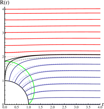
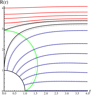
Figure 1: Numerical D7-brane embeddings for $k=0$ (dashed curves) and $k=0.007$ (continuous curves) corresponding to $T=0.5\pi^{-1}$(right) and $T=\pi^{-1}$(left). Green curves show the worldvolume horizon ($B=1$ and $\omega=1$).

and also $3\rho^{4}T(\rho)+4U_{3}(\rho)=U_{2}(\rho)$. Now the density action for the D7-branes is

$$\begin{split}S_{DBI}&=-{\cal{N}}\int dr\,e^{-\phi}\,g_{ss}^{3/2}\sqrt{1+\frac{(2\pi\alpha^{\prime})^{2}B^{2}}{g_{xx}^{2}}}g_{xx}^{3/2}\,\cr&\times\sqrt{(|g_{tt}|-g_{\psi\psi}\omega^{2})(g_{rr}+g_{RR}\,R^{\prime 2}+g_{rR}R^{\prime}+g^{xx}A_{z}^{\prime 2})+|g_{tt}|g_{\psi\psi}\psi^{\prime 2}},\cr S_{WZ}&=-{\cal{N}}(2\pi\alpha^{\prime})B\omega\int dr\,\frac{r^{4}}{\rho^{4}}A_{z}^{\prime},\end{split}$$ (29)

where (7) has been used. Notice that the four-form field in the background and consequently $S_{WS}$ are not corrected [24]. Comparing with (8), the $\alpha^{\prime}$-corrected action has two extra terms. The first term is $e^{-\phi}$ which is not a constant anymore and the second one is $g_{rR}R^{\prime}$ . As before we have two constants of motion, i.e. $\alpha$ and $\beta$. $\psi^{\prime}$ and $A^{\prime}_{z}$ can be eliminated in favor of $\alpha$ and $\beta$ by two successive Legendre-transformations and the action finally becomes (Appendix A). Additional details can be found in Appendix A. Similar to the previous section we numerically solve the equation of motion for $R(r)$ and the resulting solutions are shown in Fig. 1.

The position of $\alpha^{\prime}$-corrected worldvolume horizon on the D7-branes, $\rho_{*}$, can be found by solving (36a). In Fig. 2(right) we assume different values for $k$ and plot the worldvolume horizon in terms of $k$. It is obviously seen that by increasing $k$ the value of $\rho_{*}$ also increases. Moreover notice that $R(r_{*}=1)$ is zero for both worldvolume and AdS-Schwarzschild horizon meaning that these two horizons are coincidence at $r_{*}=1$ for small values of $k$. This fact can be obtained by using (36a). Setting $R_{*}=0$ we have

$$\frac{\gamma^{2}}{2}\frac{f(r_{*})^{2}}{H(r_{*})}\left(1-\frac{5kU_{1}(r_{*})}{r_{*}^{20}H(r_{*})^{6}}\right)=0.$$ (30)

For permitted $k$, the term in the parentheses does not vanish and therefore $f(r_{*})$ must be zero leading to $r_{*}=1$.

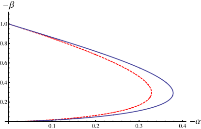
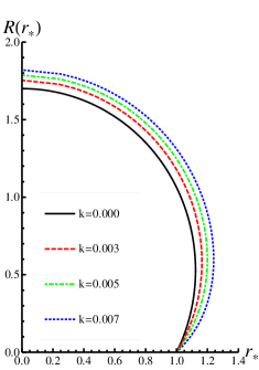
Figure 2: (Left) The blue, continuous curve shows $\alpha^{\prime}$-corrected case ($k=0.007$). (Right) The worldvolume horizon on the D7-branes for different values of $k$ ($B=1$, $\omega=1$ and $T=\pi^{-1}$) .

Each point on the worldvolume horizon, to be more specific $r_{*}$ and $R_{*}$, fixes a specific value for $\alpha$ and $\beta$. The dashed,red curve in Fig. 2(left) shows that for a given value of $\alpha$ one gets two $\beta$s. In the simplest case ( i.e. assuming $\alpha=0$) we find two options: $r_{*}=0$ or $R_{*}=0$ (see (16b) and (16c)). The former describes a solution with $\beta=0$ and the latter is a massless solution. Therefore the minimum and the maximum values of CME are given by $\alpha=0$. Since $\alpha$ ia equal to zero these solutions are CT invariant. Notice that in this figure the value of $\beta$ is normalized to the value in (17). (36b) and (36c) show that the same argument is also true for the $\alpha^{\prime}$-corrected background (the continuous, blue curve in the Fig. 2(left)).

Using the action (Appendix A) one can compute the values of $\alpha$ and $\beta$ and also the position of worldvolume horizon. The resulting expressions for $\alpha$ and the worldvolume horizon are so lengthy (see Appendix A) and hence we here explicitly state the value of $\beta$

$$\beta=-(2\pi\alpha^{\prime}){\mathcal{N}}B\omega\frac{r_{*}^{4}}{\rho_{*}^{4}}.$$ (31)

The value of $\beta$ does not explicitly depend on $\alpha^{\prime}$-correction. The reason is that the WZ term in the action is not affected by $\alpha^{\prime}$-correction. Since the position of worldvolume horizon varies, the magnitude of $\beta$ also changes. As it is clear from Fig. 4(right), the value of CME, $\langle J^{z}\rangle=-(2\pi\alpha^{\prime})\beta$, rises by $\alpha^{\prime}$-correction for the massive solutions and this increase is more considerable for higher temperatures. Note also that as it was discussed in (30) this value dose not vary for the massless solutions.

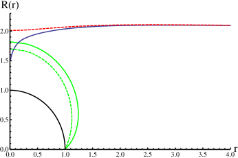
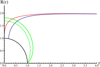
Figure 3: (Left) In the case of $m=2.037$, a Minkowski embedding without horizon for $k=0$ modifies to a Minkowski embedding with horizon for $k=0.007$. This happens for a range of masses between $m=2.028$ and $m=2.038$. (Right) A Minkowski embedding with horizon for $k=0$ modifies to a black hole embedding for $k=0.007$ when the value of $m$ is fixed by $1.912$. It happens for a range of masses between $m=1.907$ and $m=1.919$ ($B=1$, $\omega=1$ and $T=\pi^{-1}$).

At finite temperature the various embeddings of D7-branes can be classified into three groups. The Minkowski embeddings are those embeddings where the probe D7- branes close off above the horizon. In other words, the $S^{3}$ part of D7-branes shrinks to zero at an arbitrary value $\rho_{s}=R(0)>1$. Also $\rho_{s}$ can be bigger than the value of worldvolume horizon on the D7-brane, i.e. $\rho_{s}>\rho_{*}$. This group of embeddings is called Minkowski embeddings without horizon [25, 26]. In this case $\alpha$ and $\beta$ are equal to zero and there is no CME. Conversely if $\rho_{s}<\rho_{*}$, the solutions are called Minkowski embeddings with horizon. The third group is black hole embeddings [25, 26]. In this group the $S^{3}$ part of D7-branes shrinks but does not reach zero size for $\rho_{s}\geq 1$. These three groups are shown in Fig. 1 by red, black and blue curves respectively. Green curves show the worldvolume horizon in this figure. The continuous curves show the $\alpha^{\prime}$-corrected embeddings of D7-branes. As is clear from Fig. 1, for the Minkowski embeddings with horizon $R^{\prime}(0)$ is not zero and therefore such D7-branes have conical singularity (for more detail see [21]).

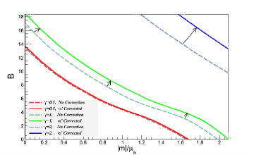
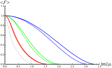
Figure 4: The red, green and blue continuous curves show the $\alpha^{\prime}$-corrected cases for $T=0.5\pi^{-1},\pi^{-1}$ and $2\pi^{-1}$, respectively ($\omega=1$). (Left) The left part of each lines in $B-m/\mu_{5}$ plot shows the region in which $\langle J^{z}\rangle$ is not zero. (Right) The value of $\langle J^{z}\rangle$ as a function of $m/\mu_{5}$. The black curve shows the zero temperature case.

In Fig. 3(left) the red, dashed curve shows a Minkowski embedding without horizon for a specified value of $m$ when the correction is not considered and the value of CME is clearly zero for this embedding. An interesting result is that in the presence of $\alpha^{\prime}$-correction the embedding becomes a Minkowski embedding with horizon (the blue, continuous curve) for the same value of mass and therefore we have a non-zero value for the CME. In other words, although before applying $\alpha^{\prime}$-correction $a(r)$ was always bigger than zero for the all values of $r$, after including $\alpha^{\prime}$-correction it becomes zero at $r=r_{*}$ and then a worldvolume horizon appears. Similarly Fig. 3(right) shows that a Minkowski embedding with horizon (the dashed, red curve) is modified into a black hole embedding (the blue, continuous curve) and as a result the conical singularity is removed by the effect of $\alpha^{\prime}$-correction. Shortly, the number of D7-brane embeddings, which gives a non-zero value for the CME, increases in the presence of $\alpha^{\prime}$-correction.

The massless solution exists for all values of the magnetic field. However, for massive solutions Fig. 4(left) shows that for a given value of the magnetic field there is a maximum value for $\frac{m}{\mu_{5}}$. In the region with $\frac{m}{\mu_{5}}<(\frac{m}{\mu_{5}})_{max}$ the value of CME is non-zero which is described by black hole embeddings or Minkowski embeddings with horizon . For $\frac{m}{\mu_{5}}>(\frac{m}{\mu_{5}})_{max}$ Minkowski embeddings without horizon exist and hence $\langle J^{z}\rangle=0$. As it is clear from Fig. 4(left) the $\alpha^{\prime}$-correction increases the value of $(\frac{m}{\mu_{5}})_{max}$. For higher temperatures the value of $(\frac{m}{\mu_{5}})_{max}$ rises. Similarly there is a $B_{max}$ for a given value of $\frac{m}{\mu_{5}}$ and for $B<B_{max}$, $\langle J^{z}\rangle\neq 0$. The $\alpha^{\prime}$-correction also increases the value of $B_{max}$.

The value of (31) can be numerically evaluated. The corresponding plot is presented in Fig. 4(right). In the massless limit the magnitude of CME, normalized to the value in (17), has a maximum value and then by increasing $\frac{m}{\mu_{5}}$ the value of CME decreases and reaches zero at $(\frac{m}{\mu_{5}})_{max}$. The continuous curves correspond to the $\alpha^{\prime}$-corrected cases. As it is clear from this figure the effect of $\alpha^{\prime}$-correction is more sensible at higher temperatures. Note also that in the case of zero temperature since the $\alpha^{\prime}$-correction does not change the $AdS_{5}\times S^{5}$ background, the value of CME is still given by (17).

4 Conclusion

Our results can be summarized as follows.

• The main result is that for massive solutions the value of CME always rises in the presence of $\alpha^{\prime}$-correction. For higher temperatures this increase is more significant. In the case of massless solution this value does not change.

• A family of D7-brane embeddings, Minkowski emmbeddings without horizon, describes solutions with no CME. The $\alpha^{\prime}$-correction changes these embeddings to the Minkowski emmbeddings with horizon where the value of CME is not zero anymore. In other words, the embeddings can be changed by the effect of $\alpha^{\prime}$-correction. It is important to notice that this happens for a range of $(\frac{m}{\mu_{5}})$s.

• Similarly, the Minkowki embeddings with horizon change into the black hole embeddings for a range of $(\frac{m}{\mu_{5}})$s in presence of the $\alpha^{\prime}$-correction. In this case both embeddings have a non-zero value for the CME. But the singularity of Minkowski embeddings with horizon is removed by the effect of $\alpha^{\prime}$-correction.

Appendix A

In order to find the equation of motion for $R(r)$, we apply two successive Legendre-transformations. The first Legendre-transformation is

$$\hat{S}_{D7}=S_{D7}-\int dr\psi^{\prime}\frac{\delta S_{D7}}{\delta\psi^{\prime}}.$$ (32)

where $S_{D7}$ is given by (29). $S_{WZ}$ does not depend on the $\psi$ and hence (32) can be written as

$$\hat{S}_{DBI} = S_{DBI}-\int dr\psi^{\prime}\,\frac{\delta S_{DBI}}{\delta\psi^{\prime}}$$

$$= -{\mathcal{N}}\int dr\,g_{ss}^{3/2}g_{xx}^{3/2}\sqrt{|g_{tt}|-g_{\psi\psi}\omega^{2}}$$

$$\times \sqrt{g_{rr}+g_{RR}\,R^{\prime 2}+g_{rR}R^{\prime}+g^{xx}A_{z}^{\prime 2}}\sqrt{1+\frac{(2\pi\alpha^{\prime})^{2}B^{2}}{g_{xx}^{2}}-\frac{\alpha^{2}/{\mathcal{N}}^{2}}{|g_{tt}|g_{\psi\psi}g_{xx}^{3}g_{ss}^{3}}},$$

where $\alpha$ is introduced in (9). The second Legendre-transformation with respect to $A^{\prime}_{z}$ is

$$\hat{\hat{S}}_{D7} = \hat{S}_{D7}-\int drA_{z}^{\prime}\frac{\delta\hat{S}_{D7}}{\delta A_{z}^{\prime}}$$

$$= -{\mathcal{N}}\int dr\sqrt{g_{rr}+g_{RR}R^{\prime 2}+g_{rR}R^{\prime}}$$

$$\times \Bigg{[}g_{xx}^{3}g_{ss}^{3}\left(|g_{tt}|-g_{\psi\psi}\omega^{2}\right)\left(1+\frac{(2\pi\alpha^{\prime})^{2}B^{2}}{g_{xx}^{2}}-\frac{\alpha^{2}/{\mathcal{N}}^{2}}{|g_{tt}|g_{\psi\psi}g_{xx}^{3}g_{ss}^{3}}\right)$$

$$- g_{xx}\left(\frac{\beta}{{\mathcal{N}}}+\frac{(2\pi\alpha^{\prime})B\omega r^{4}}{\rho^{4}}\right)^{2}\Bigg{]}^{1/2}.$$

$\beta=\frac{\delta\hat{S}_{D7}}{\delta A^{\prime}_{z}}$ and double hat means that the second Legendre transformation has been applied. Using (Appendix A) the equation of motion for $R(r)$ can be easily found and a similar analysis leading to (16) reduces to

$$\frac{\gamma^{2}}{2}\frac{f(\rho_{*})^{2}}{H(\rho_{*})} -\frac{R_{*}^{2}\omega^{2}}{\rho_{*}^{4}}$$ (36a)

$$-\frac{5k}{\rho^{20}_{*}H(\rho_{*})^{6}}\left(\frac{\gamma^{2}}{2}\frac{f(\rho_{*})^{2}U_{1}(\rho_{*})}{H(\rho_{*})}+\frac{3\omega^{2}R_{*}^{2}T(\rho_{*})}{H(\rho_{*})^{6}}\right)=0,$$

$$\beta =-(2\pi\alpha^{\prime}){\mathcal{N}}B\omega\frac{r_{*}^{4}}{\rho_{*}^{4}},$$ (36b)

$$\alpha =-\frac{1}{4}r_{*}^{3}\gamma^{4}R_{*}f(\rho_{*})H(\rho_{*})\sqrt{1+\frac{4(2\pi\alpha^{\prime})^{2}B^{2}\left(1-\frac{25kT(\rho_{*})}{\rho_{*}^{16}H(\rho_{*})^{6}}\right)}{\gamma^{4}\rho_{*}^{4}H(\rho_{*})^{2}}}$$ (36c)

$$\times\left(1+\frac{15k\text{ }T(\rho_{*})}{\rho_{*}^{16}H(\rho_{*})^{6}}\right)^{2}\sqrt{1-\frac{5k\text{ }U_{1}(\rho_{*})}{\rho_{*}^{20}H(\rho_{*})^{6}}}~{}.$$

References

- [1] J. -Y. Ollitrault, “Relativistic hydrodynamics for heavy-ion collisions,” Eur. J. Phys. 29, 275 (2008) [arXiv:0708.2433 [nucl-th]].
- [2] R. Snellings, “Elliptic Flow: A Brief Review,” New J. Phys. 13, 055008 (2011) [arXiv:1102.3010 [nucl-ex]], M. Luzum, “Flow fluctuations and long-range correlations: elliptic flow and beyond,” J. Phys. G G 38, 124026 (2011) [arXiv:1107.0592 [nucl-th]].
- [3] J. Casalderrey-Solana, H. Liu, D. Mateos, K. Rajagopal and U. A. Wiedemann, “Gauge/String Duality, Hot QCD and Heavy Ion Collisions,” arXiv:1101.0618 [hep-th].
- [4] D. Kharzeev, “Parity violation in hot QCD: Why it can happen, and how to look for it,” Phys. Lett. B 633, 260 (2006) [hep-ph/0406125].
- [5] D. Kharzeev and A. Zhitnitsky, “Charge separation induced by P-odd bubbles in QCD matter,” Nucl. Phys. A 797, 67 (2007) [arXiv:0706.1026 [hep-ph]].
- [6] D. E. Kharzeev, L. D. McLerran and H. J. Warringa, “The Effects of topological charge change in heavy ion collisions: ’Event by event P and CP violation’,” Nucl. Phys. A 803, 227 (2008) [arXiv:0711.0950 [hep-ph]].
- [7] K. Fukushima, D. E. Kharzeev and H. J. Warringa, “The Chiral Magnetic Effect,” Phys. Rev. D 78, 074033 (2008) [arXiv:0808.3382 [hep-ph]].
- [8] D. E. Kharzeev, “Topologically induced local P and CP violation in QCD x QED,” Annals Phys. 325, 205 (2010) [arXiv:0911.3715 [hep-ph]].
- [9] A. Rebhan, A. Schmitt and S. A. Stricker, “Anomalies and the chiral magnetic effect in the Sakai-Sugimoto model,” JHEP 1001, 026 (2010) [arXiv:0909.4782 [hep-th]]; H. -U. Yee, “Holographic Chiral Magnetic Conductivity,” JHEP 0911, 085 (2009) [arXiv:0908.4189 [hep-th]]; A. Gorsky, P. N. Kopnin and A. V. Zayakin, “On the Chiral Magnetic Effect in Soft-Wall AdS/QCD,” Phys. Rev. D 83, 014023 (2011) [arXiv:1003.2293 [hep-ph]]; A. Gynther, K. Landsteiner, F. Pena-Benitez and A. Rebhan, JHEP 1102, 110 (2011) [arXiv:1005.2587 [hep-th]]; T. Kalaydzhyan and I. Kirsch, “Fluid/gravity model for the chiral magnetic effect,” Phys. Rev. Lett. 106, 211601 (2011) [arXiv:1102.4334 [hep-th]].
- [10] J. M. Maldacena, “The Large N limit of superconformal field theories and supergravity,” Adv. Theor. Math. Phys. 2, 231 (1998) [hep-th/9711200], S. S. Gubser, I. R. Klebanov and A. M. Polyakov, “Gauge theory correlators from noncritical string theory,” Phys. Lett. B 428, 105 (1998) [hep-th/9802109], E. Witten, “Anti-de Sitter space and holography,” Adv. Theor. Math. Phys. 2, 253 (1998) [hep-th/9802150].
- [11] E. Witten, “Anti-de Sitter space, thermal phase transition, and confinement in gauge theories,” Adv. Theor. Math. Phys. 2, 505 (1998) [hep-th/9803131].
- [12] A. Karch and E. Katz, “Adding flavor to AdS / CFT,” JHEP 0206, 043 (2002) [hep-th/0205236].
- [13] J. Erdmenger, N. Evans, I. Kirsch and E. Threlfall, “Mesons in Gauge/Gravity Duals - A Review,” Eur. Phys. J. A 35, 81 (2008) [arXiv:0711.4467 [hep-th]].
- [14] A. Buchel, J. T. Liu and A. O. Starinets, “Coupling constant dependence of the shear viscosity in N=4 supersymmetric Yang-Mills theory,” Nucl. Phys. B 707, 56 (2005) [hep-th/0406264].
- [15] J. Noronha, M. Gyulassy and G. Torrieri, “Constraints on AdS/CFT Gravity Dual Models of Heavy Ion Collisions,” arXiv:0906.4099 [hep-ph].
- [16] N. Armesto, J. D. Edelstein and J. Mas, “Jet quenching at finite ‘t Hooft coupling and chemical potential from AdS/CFT,” JHEP 0609, 039 (2006) [hep-ph/0606245].
- [17] J. F. Vazquez-Poritz, “Drag force at finite ’t Hooft coupling from AdS/CFT,” arXiv:0803.2890 [hep-th]; K. B. Fadafan, “R**2 curvature-squared corrections on drag force,” JHEP 0812, 051 (2008) [arXiv:0803.2777 [hep-th]].
- [18] M. Ali-Akbari and K. Bitaghsir Fadafan, “Rotating mesons in the presence of higher derivative corrections from gauge-string duality,” Nucl. Phys. B 835, 221 (2010) [arXiv:0908.3921 [hep-th]].
- [19] M. Ali-Akbari and K. B. Fadafan, “Conductivity at finite ’t Hooft coupling from AdS/CFT,” Nucl. Phys. B 844, 397 (2011) [arXiv:1008.2430 [hep-th]];
- [20] K. B. Fadafan, “Strange metals at finite ’t Hooft coupling,” arXiv:1208.1855 [hep-th].
- [21] C. Hoyos, T. Nishioka and A. O’Bannon, “A Chiral Magnetic Effect from AdS/CFT with Flavor,” JHEP 1110, 084 (2011) [arXiv:1106.4030 [hep-th]].
- [22] T. Banks and M. B. Green, “Nonperturbative effects in AdS in five-dimensions x S**5 string theory and d = 4 SUSY Yang-Mills,” JHEP 9805, 002 (1998) [hep-th/9804170].
- [23] J. Pawelczyk and S. Theisen, “AdS(5) x S**5 black hole metric at O(alpha-prime**3),” JHEP 9809, 010 (1998) [hep-th/9808126].
- [24] S. S. Gubser, I. R. Klebanov and A. A. Tseytlin, “Coupling constant dependence in the thermodynamics of N=4 supersymmetric Yang-Mills theory,” Nucl. Phys. B 534, 202 (1998) [hep-th/9805156].
- [25] S. Kobayashi, D. Mateos, S. Matsuura, R. C. Myers and R. M. Thomson, “Holographic phase transitions at finite baryon density,” JHEP 0702, 016 (2007) [hep-th/0611099].
- [26] D. Mateos, S. Matsuura, R. C. Myers and R. M. Thomson, “Holographic phase transitions at finite chemical potential,” JHEP 0711, 085 (2007) [arXiv:0709.1225 [hep-th]].