Abstract

We calculate the anomalous magnetic moment of the muon in the minimal Randall-Sundrum model with standard model fields in five-dimensional (5D) warped space and a brane-localized Higgs. We use a fully 5D framework to compute the one-loop matching coefficients of the effective theory at the electroweak scale. The extra contribution to the anomalous magnetic moment from the model-independent gauge-boson exchange contributions is

$$\Delta a_{\mu}\approx 8.8\cdot 10^{-11}\,\times(1\,\mbox{TeV}/T)^{2},$$

where $1/T$ denotes the location of the TeV brane in conformal coordinates, and is related to the mass of the lowest gauge boson KK excitation by $M_{\rm KK}\approx 2.5\,T$. The result constitutes the first complete determination of the gauge-boson contribution to $g-2$ and is robust against the variation of the bulk fermion masses and 5D Yukawa coupling. We also determine the strongly model-parameter dependent effect of Higgs-exchange diagrams.

1 Introduction

The idea [1] that our four-dimensional world is one of the boundaries of a slice of strongly curved five-dimensional (5D) Anti-de-Sitter space provides an attractive approach to the gauge-gravity and flavour hierarchy problems of the Standard Model (SM). In conformal coordinates the metric of the 5D bulk is

$$ds^{2}=\left(\frac{1}{kz}\right)^{2}\left(\eta_{\mu\nu}dx^{\mu}dx^{\nu}-dz^{2}\right),$$ (1)

where $k\sim M_{\rm Pl}\sim 10^{19}\,$GeV is of order of the Planck scale $M_{\rm Pl}$, while the metric on the four-dimensional boundaries located at $z=1/k$ and $z=1/T$ is flat. This set-up provides a solution to the gauge-gravity hierarchy problem, since, if the proper distance between the two branes, $1/k\times\ln(k/T)$, is only a few times the Planck length, then $T$ can still be of order of the TeV scale. The original proposal [1] considered only gravity propagating in the bulk, but it was soon realized that the SM fields may be 5D, too [2, 3, 4, 5, 6]. An exception is the Higgs field, which in the simplest set-up is required to be localized on the TeV brane $z=1/T$ to solve the hierarchy problem. Allowing the SM fermions to propagate into the fifth dimension opens up the possibility to explain the quark and lepton mass, and the quark mixing-angle hierarchies [4, 6, 7] without postulating large hierarchies or small coupling constants in the 5D theory.

The model predicts Kaluza-Klein (KK) excitations of the SM particles with typical KK mass $M_{\rm KK}\sim 2.5\,T$ for the first excitation. The collider physics and flavour phenomenology of these KK excitations has been extensively studied. Direct searches at the Large Hadron Collider lead to lower limits on $M_{\rm KK}$ similar to those for Drell-Yan like single production of heavy resonances, which are now in the 1 to 2 TeV region. Indirect constraints from electroweak precision observables and flavour require higher KK masses, but may be avoided by adding custodial protection or flavour structure. The overwhelming number of studies is based on investigating the implications of tree-level production or tree-level exchange of the KK excitations.

Comparatively little is known about the Randall-Sundrum (RS) model at the loop level due to the intricacies of quantum field theory in curved space-times. It appears that contrary to 5D theories with a flat compact extra dimension, the running of gauge couplings is only logarithmic [8, 9, 10, 11]. Divergences associated with the fifth dimension show up in divergent KK sums. The interpretation of these divergences is not as straightforward as in Minkowski space. A precise regularization scheme, required to be able to calculate finite renormalizations, has not yet been developed. At the same time, there are a number of processes of much interest for searching for deviations of the SM, which arise only at the loop level; among them are the anomalous magnetic moment of the muon, and electromagnetic dipole transitions in the lepton ($\mu\to e\gamma$) and the quark sectors ($b\to s\gamma$), which have been considered in the RS model in [12] and [14, 15, 16, 17, 18], respectively. Higgs production through gluon-gluon fusion has been discussed in [19, 20, 21].

The systematics of renormalization and the calculation of loop processes is probably easier to approach from the 5D perspective [9, 16] instead of the KK decomposition of the dependence on the fifth coordinate. In this paper we set up the propagator and vertex Feynman rules for the 5D quantum field theory in a slice of Anti-de-Sitter (AdS) space (in this part there is significant overlap with [16]) and then revisit the muon anomalous magnetic moment as our first application. There is only one previous calculation of $(g-2)_{\mu}$ in the RS model [12], which is based on summing over towers of KK excitations. Since $(g-2)_{\mu}$ is not ultraviolet (UV) sensitive, it is well suited to demonstrate the workings of the 5D formalism without the complications of divergences from the Planck scale. The main result of the present paper is a complete calculation of $(g-2)_{\mu}$, since, as will be explained, our result differs considerably from [12].

The outline of the paper is as follows. In Sec. 2 we set up notations by defining the 5D theory and explain our strategy for calculating the anomalous magnetic moment. We match the 5D theory to an effective 4D theory, in which the scale $T$ is integrated out, keeping the relevant SU(2)$\times$U(1) invariant dimension-6 operators that must be added to the SM. After expressing the Lagrangian in terms of the fields in the electroweak vacuum, we calculate the non-standard contribution to $(g-2)_{\mu}$ in the 4D effective theory. The matching coefficients of the dimension-6 operators are computed in Sec. 3. We work with 5D fields and avoid multiple sums over KK modes by integrating out directly the fifth dimension. We identify two relevant contributions, related to the electromagnetic dipole transition and a four-fermion operator. The actual integrations must be performed numerically. We focus on the contributions to the muon anomalous magnetic moment from gauge-boson exchange. At the end of Sec. 3 we also consider genuine Higgs-exchange diagrams, whose calculation requires taking an appropriate limit of a model with a slightly brane-delocalized Higgs field. We argue that in models with anarchic Yukawa matrices Higgs-exchange is always small relative to gauge-boson exchange due to constraints from lepton-flavour-violating observables. The numerical result for the gauge-boson contributions to $(g-2)_{\mu}$ in the single-flavour approximation is shown in Sec. 4. We also discuss the dependence of the result on the bulk mass and 5D Yukawa coupling and the generalization to the case with three lepton flavours, and we compare our result to previous ones. We conclude in Sec. 5. The Feynman rules of the 5D theory are summarized in Appendices A and B, and in Appendix C we provide the explicit expressions of all diagrams for reference.

2 From the 5D theory to $(g-2)_{\mu}$

In this section we define the 5D theory, and then discuss the 4D effective Lagrangian at scales below $T$ relevant to electroweak and flavour physics when $M_{\rm EW}\ll T$. We then calculate the muon anomalous magnetic moment

$$a_{\mu}=\frac{g_{\mu}-2}{2}=a_{\mu}^{\rm SM}+\Delta a_{\mu},$$ (2)

in the effective theory, that is, we express the non-standard contributions $\Delta a_{\mu}$ in terms of the matching coefficients of higher-dimension operators in the effective Lagrangian.

2.1 The 5D theory

We adopt the simplest set-up for the SM in the RS geometry (1), in which all fields except the Higgs doublet can propagate in the bulk, and no further structure is added. While not the most attractive model for phenomenology since the scale $T$ must be quite large due to the lack of custodial protection, it provides the appropriate starting point for the study of loop processes. Quarks and the entire strong interaction sector are not relevant to leptonic processes at one-loop. In the following we specify only the SU(2)$\times$U(1) interactions and leave out the quark sector.

The 5D theory is defined by the action

$$S_{\rm(5D)} = \int d^{4}x\int\nolimits_{1/k}^{1/T}dz\,\sqrt{G}\;\Bigg{\{}\!-\frac{1}{4}F^{MN}F_{MN}-\frac{1}{4}W^{a,MN}W_{MN}^{a}$$ (3)

$$+\,\sum_{\psi=E,L}\left(e^{M}_{m}\left[\frac{i}{2}\,\bar{\psi}_{i}\,\Gamma^{m}(D_{M}-\overleftarrow{D}_{M})\psi_{i}\right]-M_{\psi_{i}}\bar{\psi}_{i}\psi_{i}\right)\Bigg{\}}+\,S_{\rm GF+ghost}$$

$$+\,\int d^{4}x\,\bigg{\{}(D^{\mu}\Phi)^{\dagger}D_{\mu}\Phi-V(\Phi)-\left(\frac{T}{k}\right)^{\!3}\left[y_{ij}^{\rm(5D)}(\bar{L}_{i}\Phi)E_{j}+\mbox{h.c.}\right]\bigg{\}},$$

where $G=1/(kz)^{10}$ is the determinant of the 5D metric and $e^{M}_{m}=kz\,\mbox{diag}\,(1,1,1,1,1)$ the inverse vielbein. The potential is given by

$$V(\Phi)=-\mu^{2}_{\rm(5D)}\left(\frac{T}{k}\right)^{\!2}\Phi^{\dagger}\Phi+\frac{\lambda}{4}\,(\Phi^{\dagger}\Phi)^{2}\,.$$ (4)

The covariant derivative is defined as usual by

$$D_{M}=\partial_{M}-ig_{5}^{\prime}\frac{Y}{2}B_{M}-ig_{5}T^{a}W^{a}_{M}.$$ (5)

$Y$ is the hypercharge of the field and $T^{a}$ the SU(2) generator in the given field representation ($\tau^{a}/2$ with $\tau^{a}$ the Pauli matrices for the doublets $L_{i}$, $\Phi$, and 0 for the singlets $E_{i}$). The hypercharge and SU(2) field strengths read

$$F_{NM}=\partial_{N}B_{M}-\partial_{M}B_{N}\qquad W_{NM}^{a}=\partial_{N}W_{M}^{a}-\partial_{M}W_{N}^{a}+g_{5}\epsilon^{abc}W_{N}^{b}W_{M}^{c}\,.$$ (6)

The Higgs doublet is localized at $z=1/T$ and described by a four-dimensional field. The powers of $(T/k)$ in the Higgs action arise from making the kinetic term canonical when the $z$-integration in the original 5D action is eliminated using the $\delta(z-1/T)$ factor. The 5D lepton fields in the lepton-Higgs Yukawa interaction are therefore evaluated at $z=1/T$. Latin indices from the middle of the alphabet refer to lepton flavour.

The dimensionful parameters $g_{5},g^{\prime}_{5},M_{\psi_{i}},y_{ij}^{\rm(5D)}$ of the Lagrangian are all of order $M_{\rm Pl}$. It is conventional to introduce the dimensionless quantities $c_{\psi_{i}}=M_{\psi_{i}}/k$ for the bulk fermion masses, whose precise values determine the hierarchical masses of the known leptons. The 5D action is given in the flavour basis that renders the bulk mass matrix diagonal, which can always be arranged by a field rotation. It is not possible in general to simultaneously diagonalize the 5D Yukawa coupling matrix $y_{ij}^{\rm(5D)}$. Unlike the SM, the 5D theory violates lepton flavour conservation and CP-symmetry in the lepton sector.

The Feynman rules for the Higgs propagator and vertices involving the Higgs field can be read off directly from (3) in the standard way. The rules for the 5D fields in the bulk of AdS are discussed and summarized in Appendix A.

2.2 Integrating out the KK scale

We assume that the scale $T$ is much larger than the masses of the SM electroweak gauge bosons and the Higgs boson. In this case we may integrate out the fifth dimension, that is, the towers of KK states to obtain an effective four-dimensional theory. Since the states with masses below $T$ are precisely represented by the SM fields, the four-dimensional theory is the SM plus SU(3)$\times$SU(2)$\times$U(1) invariant higher-dimension operators.

An issue that arises here is that the 5D theory is non-renormalizable and must itself be defined as an effective theory below a scale $\Lambda$ that should be at least a few times the Planck scale. It is generally believed that in the mixed representation the four-dimensional loop momenta should be cut-off at a value $\Lambda(z)$ that depends on the position $z$ in the fifth dimension. If $\Lambda(1/k)$ is a few times the Planck scale, then the cut-off $\Lambda(1/T)$ relevant to processes dominated by physics near the TeV brane should be near the TeV scale. This would render the naive application of the 5D formalism problematic, since it encodes the sum over all KK states rather than including only the few below the cut-off $\Lambda(1/T)$. However, for a finite quantity such as the anomalous magnetic moment of the muon, the KK sum must converge, and the effect of including the entire tower relative to the truncation is of order $T^{2}/\Lambda(1/T)^{2}$, which is the generic size of corrections expected from the UV completion of the RS model.

The dominant non-standard effects in the expansion in $M_{\rm EW}/T$ are associated with dimension-6 operators. We write

$${\cal L}_{\rm RS}^{\rm(5D)}\quad\longrightarrow\quad{\cal L}_{\rm eff}={\cal L}_{\rm SM}+\frac{1}{T^{2}}\sum_{i}c_{i}{\cal O}_{i}.$$ (7)

Since the matching coefficients $c_{i}$ are dominated by distances $\ll 1/T$, the Higgs bilinear term in $V(\Phi)$ can be treated as a perturbation, and the $c_{i}$ can be computed in the theory with unbroken electroweak gauge symmetry.

The effective Lagrangian is a special case of the general SU(3)$\times$SU(2)$\times$U(1) invariant theory with SM field content including dim-6 operators [22]. Since the anomalous magnetic moment is generated only at the one-loop level, we distinguish two types of operators.

Class-0 — operators in ${\cal L}_{\rm eff}$ that contribute to $a_{\mu}$ at tree-level, but whose short-distance coefficients are generated in the RS model only at the one-loop order. The only relevant terms are

$$\sum_{i}c_{i}{\cal O}_{i}{}_{|\,\rm class-0}=a_{B,ij}\,\bar{L}_{i}\Phi\sigma_{\mu\nu}E_{j}B^{\mu\nu}+a_{W,ij}\,\bar{L}_{i}\tau^{a}\Phi\sigma_{\mu\nu}E_{j}\,W^{a,\mu\nu}+\mbox{h.c.}$$ (8)

Note that we use the same notation for the 5D and 4D fermion and gauge fields. It is understood that the fields in the 4D effective Lagrangian correspond to the zero modes in the KK decomposition of the 5D fields. The general effective Lagrangian also contains the chirality changing operators $(\bar{L}D_{\mu}E)D^{\mu}\Phi$ and $(\bar{L}\overleftarrow{D}_{\mu}E)D^{\mu}\Phi$, but they do not generate anomalous magnetic couplings of the photon at tree level. After replacing $\Phi$ by its vacuum expectation value, the operators are $(\bar{L}_{2}\partial_{\mu}E)[D^{\mu}]_{22}$ and $(\bar{L}_{2}\overleftarrow{\partial}_{\mu}E)[D^{\mu}]_{22}$. Since $[D^{\mu}]_{22}$ contains only the $Z$-boson, this contributes to the anomalous magnetic couplings of the $Z$-boson but not the photon. The dimensionless coefficients $a_{B,W}$ are of order $g_{5}^{3}y_{ij}^{\rm(5D)}k^{5/2}$, where here $g_{5}$ denotes a generic 5D gauge coupling. Since the anomalous magnetic moment is generated only at one loop, we may use the tree-level relation

$$\frac{1}{g^{2}(\mu)}=\frac{\ln(k/T)}{g_{5}^{2}k}$$ (9)

between the 5D coupling and the 4D coupling at a scale $\mu$ of order $T$. Corrections to this relation are of order $1/(4\pi^{2})$, which counts a higher-order effect in the weak-coupling expansion. Class-1 — operators in ${\cal L}_{\rm eff}$ that contribute to $a_{\mu}$ only at the one-loop level, but which are generated in the RS model at tree-level. The relevant terms are

$$\sum_{i}c_{i}{\cal O}_{i}{}_{|\,\rm class-1} = b_{ij}\,(\bar{L}_{i}\gamma^{\mu}L_{i})(\bar{E}_{j}\gamma_{\mu}E_{j})+c_{1,i}\,(\bar{E}_{i}\gamma_{\mu}E_{i})(\Phi^{\dagger}iD^{\mu}\Phi)$$ (10)

$$+\,c_{2,i}\,(\bar{L}_{i}\gamma_{\mu}L_{i})(\Phi^{\dagger}iD^{\mu}\Phi)+c_{3,i}\,(\bar{L}_{i}\gamma^{\mu}\tau^{a}L_{i})(\Phi^{\dagger}\overleftrightarrow{i\tau^{a}D_{\mu}}\Phi)\;,$$

where $\overleftrightarrow{i\tau^{a}D_{\mu}}=1/2\,(i\tau^{a}D_{\mu}-i\overleftarrow{D}_{\mu}\tau^{a})$. They are generated at tree-level by the exchange of the 4D vector components of the KK gauge bosons. Although the 5D gauge couplings to fermions are flavour-diagonal and universal, flavour-dependence of the coefficient functions arises through the different zero-mode profiles of the 4D fermions. The operators $(\bar{L}_{i}D_{\mu}E_{j})D^{\mu}\Phi$ and $(\bar{L}_{i}\overleftarrow{D}_{\mu}E_{j})D^{\mu}\Phi$ discussed already above might contribute to the photon anomalous magnetic moment at the one-loop level, but inspection shows that it cannot be generated at tree-level from integrating out the KK scale. Another class-1 operator that could possibly contribute to $g-2$ is $\bar{L}_{i}\Phi E_{j}\Phi^{\dagger}\Phi$ (and its hermitian conjugate). It can only be generated at tree level by diagrams with three Yukawa couplings. In scenarios with an (approximately) brane localized Higgs field these diagrams are non-vanishing only when one includes the “wrong-chirality” Higgs couplings of the fermions [23]. For simple Higgs profiles these terms can be calculated fully analytically in the limit that the width of the Higgs profile around the TeV brane is taken to zero. We will discuss these terms separately in Sec. 3.4 and therefore do not include $\bar{L}_{i}\Phi E_{j}\Phi^{\dagger}\Phi$ in (10). KK gauge boson exchange also generates further four-fermion operators with only left-handed and only right-handed fields, but these do not contribute to the anomalous magnetic moment. The mixed left-right lepton-quark operator $(\bar{L}E)(\bar{Q}U)$, on the other hand, does contribute at one loop, but it is not generated in the RS model. Other class-1 operators that one might write down contribute to $a_{\mu}$ only indirectly, through a modification of the relation of the SM parameters to those of the 5D theory. When expressing the SM contribution to $a_{\mu}$ in terms of SM parameters, this effect is already accounted for. Thus (10) represents the complete list of relevant operators. The coefficient functions $b,c_{1,2,3}$ are of order $g_{5}^{2}k$. In particular, we note the presence of chirality-preserving fermion-Higgs interactions proportional to 5D gauge rather than Yukawa couplings.

We now express the effective Lagrangian in terms of the fields in the electroweak vacuum, in which the SU(2)$\times$U(1) gauge symmetry is spontaneously broken to electromagnetism. Thus, we replace

$$\Phi\to\left(\begin{array}[]{c}\phi^{+}\\ \frac{1}{\sqrt{2}}(v+H+iG)\end{array}\right),$$ (11)

and

$$D_{\mu}\to\partial_{\mu}-ieQA_{\mu}-i\frac{g}{c_{W}}(T^{3}-s^{2}_{W}Q)Z_{\mu}-i\frac{g}{\sqrt{2}}(T^{1}+iT^{2})W^{+}_{\mu}-i\frac{g}{\sqrt{2}}(T^{1}-iT^{2})W^{-}_{\mu},$$ (12)

where $c_{W}\,(s_{W})$ is the cosine (sine) of the Weinberg angle, with $c_{W}^{2}=g^{2}/(g^{2}+g^{\prime\,2})$. For the fermions it is convenient to transform to the mass basis, in which the effective Yukawa interaction $-y_{ij}\bar{L}_{i}\Phi E_{j}$ of the 4D fields is diagonal. Tree-level matching results in the 4D Yukawa coupling

$$y_{ij} = \left(\frac{T}{k}\right)^{\!3}f^{(0)}_{L_{i}}(1/T)g^{(0)}_{E_{j}}(1/T)\,y_{ij}^{\rm(5D)}$$ (13)

$$= \sqrt{\frac{1-2c_{L_{i}}}{1-(T/k)^{1-2c_{L_{i}}}}}\,\sqrt{\frac{1+2c_{E_{j}}}{1-(T/k)^{1+2c_{E_{j}}}}}\,y_{ij}^{\rm(5D)}k\,$$

where $f^{(0)}_{L_{i}}(z)$ and $g^{(0)}_{E_{j}}(z)$ are the fermion zero-mode profiles, see appendix A. The transition to the mass basis is given by the unitary rotations

$$L_{i}\to U_{ij}L_{j},\qquad E_{i}\to V_{ij}E_{j}$$ (14)

of the 4D fields in ${\cal L}_{\rm eff}$. To go to the broken theory,

$$E_{i}\to V_{ij}P_{R}\psi_{j},\qquad L_{i}\to U_{ij}P_{L}\!\left(\begin{array}[]{c}\nu_{j}\\ \psi_{j}\end{array}\right),$$ (15)

where $\psi_{i}$ is the Dirac spinor field for the massive leptons ($i=1,2,3$ corresponding to electron, muon, tau) and $\nu_{i}$ is the corresponding neutrino spinor field. $P_{L/R}=(1\mp\gamma_{5})/2$ are the chiral projectors. Inserting these substitutions into (8), (10), generates numerous different operators composed of SM fields. We neglect operators which cannot contribute to the magnetic and electric dipole form factors or only start contributing at two loops. The effective Lagrangian for the computation of the anomalous magnetic (and electric) moments, as well as charged lepton-flavour violating processes at one loop is then given by

$$\sum_{i}c_{i}{\cal O}_{i} \to \frac{\alpha_{ij}+\alpha_{ji}^{*}}{2}\frac{v}{\sqrt{2}}\,\bar{\psi}_{i}\sigma_{\mu\nu}\psi_{j}F^{\mu\nu}+\frac{\alpha_{ij}-\alpha_{ji}^{*}}{2i}\,\frac{v}{\sqrt{2}}\,\bar{\psi}_{i}\sigma_{\mu\nu}i\gamma_{5}\psi_{j}F^{\mu\nu}$$ (16)

$$+\,\beta_{ijkl}\,(\bar{\psi}_{i}\gamma^{\mu}P_{L}\psi_{j})(\bar{\psi}_{k}\gamma_{\mu}P_{R}\psi_{l})$$

$$+\,\gamma_{1,ij}\,\frac{v}{2}\,(\bar{\psi}_{i}P_{L}\gamma_{\mu}\psi_{j})(i\partial^{\mu}H)+[\gamma_{2,ij}+\gamma_{3,ij}]\,\frac{v}{2}\,(\bar{\psi}_{i}P_{R}\gamma_{\mu}\psi_{j})(i\partial^{\mu}H)$$

$$+\,\gamma_{3,ij}\,\frac{v}{\sqrt{2}}(\bar{\psi}_{i}P_{R}\gamma_{\mu}\nu_{j})(-i\partial^{\mu}\phi^{-})+\gamma_{3,ij}\,\frac{v}{\sqrt{2}}(\bar{\psi}_{i}P_{R}\gamma_{\mu}\nu_{j})(eA^{\mu}\phi^{-})$$

$$+\,\mbox{ h.c. of previous line}$$

with $F_{\mu\nu}$ the photon field strength tensor. The couplings are

$$\alpha_{ij} = [U^{\dagger}aV]_{ij},$$

$$\beta_{ijkl} = \sum_{m,n}\,[U^{\dagger}]_{im}U_{mj}[V^{\dagger}]_{kn}V_{nl}\,b_{mn},$$

$$\gamma_{1,ij} = \sum_{m}\,[V^{\dagger}]_{im}V_{mj}\,c_{1,m},$$

$$\gamma_{x,ij} = \sum_{m}\,[U^{\dagger}]_{im}U_{mj}\,c_{x,m}\quad(x=2,3)$$ (17)

with $a_{ij}=c_{W}a_{B,ij}-s_{W}a_{W,ij}$. Many further terms can in principle appear on the right-hand side of (16) upon replacing the fields in ${\cal O}_{i}$ by those of the broken theory. Inspection shows that these additional terms are not relevant, since they contribute only to the form factor $F_{1}$, see (18) below, or to $F_{2}$ and the magnetic moment only beyond one loop.

2.3 The muon anomalous magnetic moment

The muon-photon vertex function is given by

$$\Gamma^{\mu}(p,p^{\prime})=ieQ_{\mu}\,\bar{u}(p^{\prime},s^{\prime})\left[\gamma^{\mu}F_{1}(q^{2})+\frac{i\sigma^{\mu\nu}q_{\nu}}{2m_{\mu}}F_{2}(q^{2})+\ldots\right]u(p,s)$$ (18)

where the ellipses denote parity-violating terms, and $q=p^{\prime}-p$. The factor $ieQ_{\mu}$ with $Q_{\mu}=-1$ corresponds to our definition of the gauge covariant derivative and the standard normalization of the charge form factor $F_{1}(0)=1$. The anomalous magnetic moment is defined by

$$a_{\mu}=\frac{(g-2)_{\mu}}{2}=F_{2}(0).$$ (19)

It is straightforward to compute the extra contribution $\Delta a_{\mu}$ from the effective Lagrangian (16). Since $\alpha$ is a one-loop quantity, while $\beta$ and $\gamma_{x}$ are tree-level, we need to compute the diagrams shown in figure 1.

Figure 1: Diagrams for $a_{\mu}$ from (16).

The tree-level diagram (a) with an insertion of the class-0 electromagnetic dipole operator results in

$$\Gamma^{\mu}(p,p^{\prime})=\frac{1}{T^{2}}\,\mbox{Re}\,(\alpha_{22})\,\,\frac{v}{\sqrt{2}}\,2i\,\bar{u}(p^{\prime},s^{\prime})i\sigma^{\mu\nu}q_{\nu}u(p,s).$$ (20)

The imaginary part of the $\alpha_{ij}$ couplings generates an electric dipole moment.

There are two possible contractions of the four-fermion operator (diagram (b)), which differ by the exchange of $P_{L}\leftrightarrow P_{R}$ and $\beta_{2kk2}\leftrightarrow\beta_{k22k}$. The loop integral is ultraviolet (UV) divergent by power counting and must be regularized. The divergence is related to factorization of the contributions from the KK scale $T$ and the low-energy scales $m_{\ell}$, which is the only scale present in diagram (b) from the external momenta and massive lepton propagators. We adopt dimensional regularization with $d=4-2\varepsilon$. The final result is finite, and arises from the UV $1/\varepsilon$ pole that multiplies a numerator of ${\cal O}(\varepsilon)$. It depends on the scheme and we use the “naive dimensional regularization” (NDR) scheme with anti-commuting $\gamma_{5}$. The scheme dependence of this ultraviolet-sensitive term is compensated by a corresponding dependence in the calculation of the matching coefficients as we discuss later. The situation is similar to the calculation of the $b\to s\gamma$ transition with the weak effective Lagrangian method.

The contribution to the vertex function from the four-fermion operator in the effective Lagrangian is

$$\Gamma^{\mu}(p,p^{\prime}) = \frac{i\beta_{2kk2}}{T^{2}}\,ieQ_{\ell_{k}}\,\mu^{2\varepsilon}\!\int\!\frac{d^{d}l}{(2\pi)^{d}}\,\frac{\bar{u}(p^{\prime},s^{\prime})\gamma^{\rho}P_{L}i(l\hskip-4.49997pt/+m_{\ell_{k}})\gamma^{\mu}i(l\hskip-4.49997pt/-q\hskip-4.49997pt/+m_{\ell_{k}})\gamma_{\rho}P_{R}u(p,s)}{(l^{2}-m_{\ell_{k}}^{2})((l-q)^{2}-m_{\ell_{k}}^{2})}$$ (21)

$$+\,(\beta_{2kk2}\leftrightarrow\beta_{k22k},\,P_{L}\leftrightarrow P_{R})$$

$$= -ieQ_{\mu}\,\frac{m_{\ell_{k}}}{16\pi^{2}T^{2}}\,\bar{u}(p^{\prime},s^{\prime})i\sigma^{\mu\nu}q_{\nu}\left[\beta_{2kk2}+\beta_{k22k}+(\beta_{2kk2}-\beta_{k22k})\gamma_{5}\right]u(p,s)$$

where a sum over internal lepton flavours $k=1,2,3$ is understood, and the limit $d\to 4$ has been taken. The $\gamma_{5}$ term is related to the electric dipole moment; the remaining terms are the desired contributions to the anomalous magnetic moment of the muon.

The Higgs derivative interactions from (16) contribute via the diagrams (c1), (c2) and (d1), (d2) of figure 1. Diagram (c1) with an insertion of the $\gamma_{2}$ coupling is given by

$$\Gamma^{\mu}(p,p^{\prime}) = \frac{i\gamma_{2,22}v}{2T^{2}}\,ieQ_{\mu}\,\frac{iy_{\mu}}{\sqrt{2}}\,$$ (22)

$$\times\,\mu^{2\varepsilon}\!\int\!\frac{d^{d}l}{(2\pi)^{d}}\,\frac{(+i)\,\bar{u}(p^{\prime},s^{\prime})P_{R}\,l\hskip-4.49997pt/i(p\hskip-4.49997pt/^{\prime}-l\hskip-4.49997pt/+m_{\mu})\gamma^{\mu}i(p\hskip-4.49997pt/-l\hskip-4.49997pt/+m_{\mu})u(p,s)}{(l^{2}-m_{H}^{2})((p-l)^{2}-m_{\mu}^{2})((p^{\prime}-l)^{2}-m_{\mu}^{2})}.\quad$$

Here $y_{\mu}=\sqrt{2}m_{\mu}/v$ is the small standard model muon Yukawa coupling. The prefactor is proportional to the muon mass $m_{\mu}=y_{\mu}v/\sqrt{2}$, since one of the vertices is the SM Higgs-fermion vertex. We may therefore neglect the muon mass in the integrand, and use the on-shell conditions to obtain

$$\Gamma^{\mu}(p,p^{\prime}) = -\frac{i\gamma_{2,22}m_{\mu}}{2T^{2}}\,ieQ_{\mu}\,\mu^{2\varepsilon}\!\int\!\frac{d^{d}l}{(2\pi)^{d}}\,\frac{\bar{u}(p^{\prime},s^{\prime})P_{R}\gamma^{\mu}(-l\hskip-4.49997pt/)u(p,s)}{(l^{2}-m_{H}^{2})(l^{2}-2p\cdot l)}.$$ (23)

This vanishes, since the loop integral can only result in $p\hskip-4.49997pt/u(p,s)=0$. Diagram (c2) and the insertions of the $\gamma_{1,3}$ interactions vanish in an analogous way. The reason for this can be deduced without calculations from the operator $\bar{\psi}P_{L/R}\gamma_{\mu}\psi\partial^{\mu}H$, which, up to a total derivative, can be converted into $\partial^{\mu}(\bar{\psi}P_{L/R}\gamma_{\mu}\psi)H$. In the NDR scheme, by the field equations, this operator is proportional to lepton masses, or small coupling constants, and hence of higher-order in our approximations. The corresponding arguments cannot be applied in the unbroken theory, since there the operator contains two Higgs fields.

Diagrams (d1) and (d2) involve an internal charged Higgs and a neutrino line. For diagram (d1) we find

$$\Gamma^{\mu}(p,p^{\prime}) = \frac{i\gamma_{3,22}v}{\sqrt{2}T^{2}}\,(ie)\,(-iy_{\mu})$$ (24)

$$\times\,\mu^{2\varepsilon}\!\int\!\frac{d^{d}l}{(2\pi)^{d}}\,\frac{i^{2}\,\bar{u}(p^{\prime},s^{\prime})\,P_{R}(l\hskip-4.49997pt/-p\hskip-4.49997pt/^{\prime})i(l\hskip-4.49997pt/+m_{\nu})P_{R}u(p,s)\;(2l-p-p^{\prime})^{\mu}}{((p-l)^{2}-m_{\phi}^{2})((p^{\prime}-l)^{2}-m_{\phi}^{2})(l^{2}-m_{\nu}^{2})}\;.\quad$$

The prefactor is proportional to the muon mass, hence we can neglect the muon and neutrino mass in the remainder of the expression. Introducing the Feynman parameter $x$ ($\bar{x}=1-x$) to combine denominators leads to

$$\Gamma^{\mu}(p,p^{\prime}) = -\frac{e\gamma_{3,22}m_{\mu}}{T^{2}}\,$$ (25)

$$\times\,\mu^{2\varepsilon}\!\int\!\frac{d^{d}l}{(2\pi)^{d}}\,\int_{0}^{1}dx\frac{\bar{u}(p^{\prime},s^{\prime})P_{R}u(p,s)\;(p+p^{\prime}-2l)^{\mu}}{((l-x\,p-\bar{x}\,p^{\prime})^{2}-m_{\phi}^{2}+xp^{2}+\bar{x}{p^{\prime}}^{2}-(xp+\bar{x}p^{\prime})^{2})^{2}}$$

$$= -\frac{e\gamma_{3,22}m_{\mu}}{T^{2}}\,\mu^{2\varepsilon}\!\int\!\frac{d^{d}l}{(2\pi)^{d}}\int_{0}^{1}\!dx\frac{\bar{u}(p^{\prime})P_{R}u(p)[(\bar{x}-x)p^{\mu}+(x-\bar{x})p^{\prime\mu}]}{(l^{2}-m_{\phi}^{2}+x\bar{x}q^{2})^{2}}$$

$$= 0\,,$$

where in the last step we used that the integrand is antisymmetric under the exchange $x\leftrightarrow\bar{x}$. For later purposes, we note that the zero arises due to a cancellation between a finite term and an ultraviolet-sensitive term that arises as the product $1/\varepsilon\times\varepsilon$ of a UV divergence and a numerator of ${\cal O}(\varepsilon)$. To see this, we assume $l\gg p,p^{\prime}$, expand the integrand of (24) to first order in the external momenta, and extract the $(p+p^{\prime})^{\mu}$ structure that is relevant to the magnetic moment. This results in

$$\Gamma^{\mu}(p,p^{\prime}) \stackrel{{\scriptstyle\rm UV}}{{\longrightarrow}} \frac{i\gamma_{3,22}v}{\sqrt{2}T^{2}}\,(ie)\,(-iy_{\mu})\,i\,$$ (26)

$$\times\mu^{2\varepsilon}\!\int\!\frac{d^{d}l}{(2\pi)^{d}}\frac{\bar{u}(p^{\prime},s^{\prime})P_{R}u(p,s)\,(p+p^{\prime}-2l)^{\mu}}{(l^{2}-m_{\phi}^{2})^{2}}\left(1+\frac{2p\cdot l+2p^{\prime}\cdot l}{l^{2}-m_{\phi}^{2}}\right)$$

$$\longrightarrow -\frac{ie\gamma_{3,22}m_{\mu}}{T^{2}}\,\frac{\mu^{2\varepsilon}}{(4\pi)^{d/2}}\,\left[\left(1-\frac{4}{d}\right)\times\frac{\Gamma(\varepsilon)}{m_{\phi}^{2\varepsilon}}\,(p+p^{\prime})^{\mu}+\frac{4}{d}\frac{\Gamma(1+\varepsilon)}{2m_{\phi}^{2\varepsilon}}\,(p+p^{\prime})^{\mu}\right]$$

$$\times\bar{u}(p^{\prime},s^{\prime})P_{R}u(p,s)$$

$$= \frac{ie\gamma_{3,22}m_{\mu}}{(4\pi)^{2}T^{2}}\,\bar{u}(p^{\prime},s^{\prime})P_{R}(p+p^{\prime})^{\mu}u(p,s)\times\left(\frac{\varepsilon}{2}\times\frac{1}{\varepsilon}-\frac{1}{2}\right)+{\cal O}(\varepsilon).$$

The total contribution is, of course, zero; but the contribution due to the UV pole is finite despite the superficial divergence of the integral. This will be important when verifying the scheme independence in Sec. 3.3.3. An analogous result holds for (d2).

Diagrams (e1) and (e2) follow from the insertion of the operator $\bar{\psi}_{i}P_{R}\gamma^{\mu}\nu_{j}\,(eA_{\mu}\phi^{-})$ in (16) and its hermitian conjugate, respectively. None of the two contributes to $(g-2)_{\mu}$ as the loop only depends on a single external four-momentum. We can use on-shell condition to convert each appearance of $\not{p}^{(\prime)}$ to a lepton mass. The only possible Lorentz structure is then $\bar{u}(p^{\prime},s^{\prime})\gamma^{\mu}P_{R/L}u(p,s)A_{\mu}$, which contributes only to the $F_{1}$ form factor.

The muon anomalous magnetic moment follows by adding the non-vanishing matrix elements of the dipole and four-fermion operator, (20) and (21), respectively, resulting in

$$\Delta a_{\mu} = \frac{1}{T^{2}}\,\mbox{Re}\,(\alpha_{22})\,\,\frac{1}{-e}\,\frac{4m_{\mu}v}{\sqrt{2}}+\sum_{k=1,2,3}(-1)\,\frac{2m_{\mu}m_{\ell_{k}}}{16\pi^{2}T^{2}}\,\left[\beta_{2kk2}+\beta_{k22k}\right]$$ (27)

$$= -\,\frac{4m_{\mu}^{2}}{T^{2}}\left(\frac{\mbox{Re}\,(\alpha_{22})}{y_{\mu}e}+\sum_{k=1,2,3}\frac{1}{16\pi^{2}}\,\frac{m_{\ell_{k}}}{m_{\mu}}\,\mbox{Re}\,(\beta_{2kk2})\right).$$

Here $k=1,2,3$ refers to electron, muon and tau leptons, respectively. In passing to the last line of (27), we used that $b_{mn}$, being generated by gauge interactions, is real. It therefore follows from the definitions (17) that $\beta_{k22k}=\beta_{2kk2}^{*}$, and hence $\beta_{2kk2}+\beta_{k22k}$ is real as it should be.

3 Calculation of matching coefficients

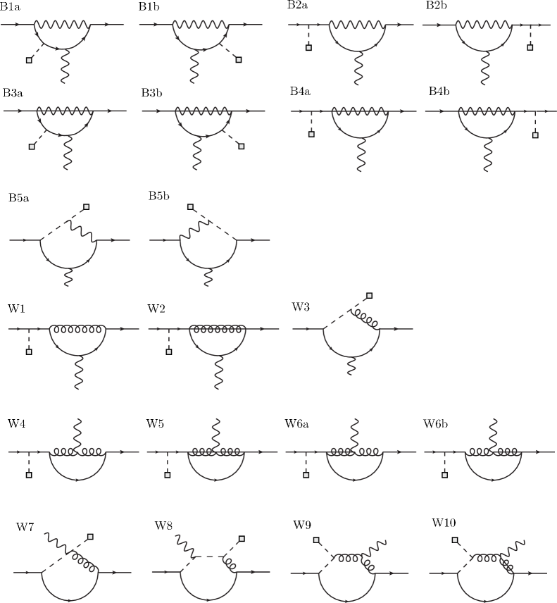
Figure 2: Diagrams contributing to $\Delta a_{\mu}$, more precisely the matching coefficients of the class-0 operators. Solid lines refer to leptons, with the right external line belonging to the doublet $L_{i}$, the left one to $E_{j}$. Wavy lines denote hypercharge gauge bosons and the external photon, curly lines SU(2) W-bosons. A solid-wavy (solid-curly) line refers to the scalar fifth component of the gauge field. Dashed lines denote Higgs bosons, including the external Higgs field (grey box). Vertices involving Higgs fields are localized at $1/T$, all other vertices are integrated over position in the fifth dimension.

We now turn to the calculation of the matching coefficients in the RS model (3). The diagrams relevant to the anomalous magnetic moment in the full 5D theory with unbroken gauge symmetry are shown in figure 2. The figure does not include genuine Higgs-exchange diagrams, which involve three Yukawa interactions (rather than one Yukawa and two gauge interactions as in figure 2), and which we discuss separately in Sec. 3.4.

In a direct calculation of $a_{\mu}$ in the 5D theory, the diagrams should be represented in terms of the fields and interactions in the expansion around the electroweak vacuum of the spontaneously broken theory, which depend on the scales $k$, $T$, $M_{\rm EW}$, $m_{\ell_{k}}$. In drawing the diagrams in figure 2 we already accounted for the fact that we only need to extract the contributions from the scales $k$ and $T$, which gives directly the short-distance coefficients of the SU(3)$\times$SU(2)$\times$U(1) invariant effective Lagrangian. The diagrams in the unbroken theory do not represent the infrared physics from the scales near and below the electroweak scale $M_{\rm EW}$ correctly, but the incorrect infrared contribution cancels in the matching procedure. The low-momentum contributions from diagrams with 5D non-zero-mode propagators have already been included through the calculations of the previous subsection. Note that we do not consider diagrams with graviton exchange; see [12, 13] for a discussion of the graviton contribution.

The diagrams are understood in the mixed representation with an integration over four-dimensional loop momentum $l$ and the vertex positions in the fifth dimension. A generic diagram such as diagram B1a in figure 2 can have three different contributions:

• All 5D propagators propagate the zero mode. The loop integral does not contain the short-distance scales $T,k$ explicitly, and is purely long-distance. This corresponds to a contribution to the SM anomalous magnetic moment $a_{\mu}^{\rm SM}$. There is no need to perform this computation here, so we subtract this contribution.

• At least one of the 5D propagators propagates a KK mode, but the loop momentum $l$ satisfies $l\ll T$. In this case, the subgraph consisting of propagators with KK modes can be contracted to a point. The reduced loop diagram must be computed with the 4D effective Lagrangian. This corresponds to tree-level matching of class-1 operators and the one-loop operator matrix element calculations performed in the previous subsection. An explicit diagrammatic analysis shows that the relevant subgraphs in figure 2 correspond precisely to the operators (10), and neglected operators of dimension higher than six. In diagram B1a, for example, the only relevant contribution occurs when the gauge boson is a KK mode and all internal fermions are zero modes, which corresponds to the insertion of a local four-fermion operator as in diagram (b) of figure 1. The fermion-Higgs effective vertex and diagram (d1) are related exclusively to diagram W8. If the gauge boson and at least one of the fermion propagators refers to a KK mode and the loop momentum is small, the contribution is suppressed and corresponds to a higher-dimension operator. If the gauge boson is the zero mode, then the flatness of the gauge zero mode and the orthogonality condition for the fermion modes forces all fermion lines to propagate zero modes as well. This is the SM contribution discussed above.

• The loop momentum is of order $l\sim T$ or larger. This contribution goes into the one-loop matching coefficients of the class-0 operators.

In the following we describe the computation of the matching coefficients mentioned in the second and third item.

3.1 Four-fermion operator

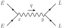
Figure 3: Hypercharge boson exchange that generates the four-fermion operator.

The tree-level matching calculation is very similar to the one that generates flavour-changing four-quark operators from KK gluon exchange[14, 24, 25, 26, 27]. Here we perform the calculation in the 5D picture, which makes it particularly simple (provided the 5D propagators are known).

The relevant diagram is shown in figure 3. Only hypercharge vector gauge boson exchange can generate the $(\bar{L}_{i}\gamma^{\mu}L_{i})(\bar{E}_{j}\gamma_{\mu}E_{j})$ operator at tree level, since SU(2) gauge fields do not interact with $E_{i}$. The scalar fifth component of the 5D gauge boson cannot be exchanged, since the two external zero-mode fermions at the vertex have the same handedness. From the tree diagram shown in figure 3, we obtain

$$b_{ij} = -i\,(ig_{5}^{\prime})^{2}\,\frac{Y_{L}}{2}\frac{Y_{E}}{2}\,T^{2}\int_{1/k}^{1/T}\!\!dxdy\,\frac{{f_{L_{i}}^{(0)}}^{2}\!(x)}{(kx)^{4}}\,\frac{{g_{E_{j}}^{(0)}}^{2}\!(y)}{(ky)^{4}}\,\Delta_{\perp}^{\rm ZMS}(q=0,x,y).$$ (28)

Here $Y_{L}=-1$, $Y_{E}=-2$ denote the hypercharges of the leptons, and $\Delta_{\perp}$ is the $\eta_{\mu\nu}$ component of the 5D gauge boson propagator given in (155) of the appendix (see also [9]). We subtracted the zero mode from the propagator, since this corresponds to a SM contribution to $a_{\mu}$.

Because of the large mass of the KK excitations, the external lepton momenta of order $m_{\mu}$ can be set to zero. The zero-momentum limit of the gauge-boson propagator (155) is

$$\Delta_{\perp}(q,x,y) \stackrel{{\scriptstyle q\to 0}}{{=}} \Theta(x-y)\,\frac{ik}{\ln\frac{k}{T}}\,\bigg{(}-\frac{1}{q^{2}}+\frac{1}{4}\,\bigg{\{}\frac{1/T^{2}-1/k^{2}}{\ln\frac{k}{T}}-x^{2}-y^{2}+2x^{2}\ln(xT)$$ (29)

$$+\,2y^{2}\ln(yT)+2y^{2}\ln\frac{k}{T}\bigg{\}}+{\cal O}(q^{2})\bigg{)}+(x\leftrightarrow y),$$

which agrees with a similar expression obtained in [26] from the explicit summation over all KK excitations. The $1/q^{2}$ term is evidently the zero mode. Subtracting it, neglecting $1/k^{2}$ relative to $1/T^{2}$ in the first term in curly brackets, since $\epsilon\equiv T/k\sim 10^{-16}$ is very small, and employing the normalization (99) of the zero modes, we obtain

$$b_{ij} = -\frac{1}{4}{g^{\prime}}^{2}\,\frac{Y_{L}}{2}\frac{Y_{E}}{2}\,T^{2}\,\Bigg{(}\frac{1}{T^{2}\ln\frac{k}{T}}$$ (30)

$$+\,\int_{1/k}^{1/T}\!\!dx\,\frac{{f_{L_{i}}^{(0)}}^{2}\!(x)}{(kx)^{4}}\,x^{2}\left(2\ln(xT)-1\right)+\int_{1/k}^{1/T}\!\!dy\,\frac{{g_{E_{j}}^{(0)}}^{2}\!(y)}{(ky)^{4}}\,y^{2}\left(2\ln(yT)-1\right)$$

$$+\,2\ln\frac{k}{T}\int_{1/k}^{1/T}\!\!dxdy\,\frac{{f_{L_{i}}^{(0)}}^{2}\!(x)}{(kx)^{4}}\,\frac{{g_{E_{j}}^{(0)}}^{2}\!(y)}{(ky)^{4}}\,\mbox{min}\,(x^{2},y^{2})\Bigg{)}.$$

The remaining integrals over the fifth-dimension coordinates are dominated by $x,y\sim 1/T$ up to terms suppressed by some power of $T/k$ provided the bulk mass parameters satisfy $c_{L_{i}}<3/2$ and $c_{E_{j}}>-3/2$, which will be assumed. We can therefore set the lower integration limit to 0 and use the explicit form of the fermion zero modes from (103a), (103b) in the appendix to find

$$b_{ij}=b_{0}+b_{1}(c_{L_{i}})+b_{1}(-c_{E_{j}})+b_{2}(c_{L_{i}},c_{E_{j}})$$ (31)

with

$$b_{0}=-\frac{{g^{\prime}}^{2}}{8}\,\frac{1}{\ln(1/\epsilon)},$$

$$b_{1}(c)=-\frac{{g^{\prime}}^{2}}{8}\,\frac{(5-2c)(1-2c)}{(3-2c)^{2}}\,\frac{\epsilon^{2c-1}}{1-\epsilon^{2c-1}},$$ (32)

$$b_{2}(c_{L},c_{E})=-\frac{{g^{\prime}}^{2}}{4}\,\frac{(1-2c_{L})(1+2c_{E})(3-c_{L}+c_{E})}{(3-2c_{L})(3+2c_{E})(2-c_{L}+c_{E})}\,\ln\frac{1}{\epsilon}\,\frac{\epsilon^{2c_{L}-1}}{1-\epsilon^{2c_{L}-1}}\,\frac{\epsilon^{-2c_{R}-1}}{1-\epsilon^{-2c_{R}-1}}.$$

Substituting this result for $b_{ij}$ into (17) and exploiting the unitarity of the flavour rotation matrices to the mass basis, we obtain

$$\beta_{ijkl} = b_{0}\delta_{ij}\delta_{kl}+\delta_{kl}\sum_{m}b_{1}(c_{L_{m}})\,[U^{\dagger}]_{im}U_{mj}+\delta_{ij}\sum_{n}b_{1}(-c_{E_{n}})\,[V^{\dagger}]_{kn}V_{nl}$$ (33)

$$+\,\sum_{m,n}b_{2}(c_{L_{m}},c_{E_{n}})\,[U^{\dagger}]_{im}U_{mj}[V^{\dagger}]_{kn}V_{nl}.$$

The first term does not change lepton flavour number $F$, the next two may change $\Delta F=\pm 1$, and only the term in the second line can produce $\Delta F=\pm 2$ transitions. All terms are formally required to compute $\sum_{k}m_{\ell_{k}}/m_{\mu}\times\beta_{2kk2}$ relevant to the anomalous magnetic moment.

A particularly simple result is obtained in the “single-flavour approximation”, where we ignore the presence of other leptons than the muon. This corresponds to replacing $\sum_{k}m_{\ell_{k}}/m_{\mu}\times\beta_{2kk2}\to\beta_{2222}\equiv\beta$, and $U_{ij}=V_{ij}=\delta_{ij}$, such that

$$\beta=b_{0}+b_{1}(c_{L})+b_{1}(-c_{E})+b_{2}(c_{L},c_{E})\equiv-\frac{{g^{\prime}}^{2}}{8}\frac{1}{\ln(1/\epsilon)}\,f(\epsilon,c_{L},c_{E}).$$ (34)

Setting further $c_{L}=-c_{E}=1/2+r$ ($r>0$), we find

$$f=1-\frac{\epsilon^{2r}}{1-\epsilon^{2r}}\,\ln\frac{1}{\epsilon}\,\frac{2r(2-r)}{(1-r)^{2}}+\left[\frac{\epsilon^{2r}}{1-\epsilon^{2r}}\,\ln\frac{1}{\epsilon}\right]^{2}\,\frac{4r^{2}}{(1-r)(1-2r)}.$$ (35)

According to (13), $r$ is related to the muon mass by

$$\frac{2r\epsilon^{2r}}{1-\epsilon^{2r}}=\frac{y_{\mu}}{y_{\mu}^{\rm(5D)}k}=\frac{\sqrt{2}m_{\mu}}{y_{\mu}^{\rm(5D)}kv}.$$ (36)

With $\epsilon=10^{-16}$ and $y_{\mu}^{\rm(5D)}k=1$, we find $r=0.0749$ and $f=0.95$. In general, when $y_{\mu}^{\rm(5D)}k$ is of order 1 and $\epsilon$ within a few orders of magnitude near $10^{-16}$, the deviation of $f$ from 1 is only a few percent, and the flavour-conserving four-fermion matching coefficient is dominated by the $r$-independent term $b_{0}$. In this case the total contribution (34) is suppressed by the large logarithm $\ln(1/\epsilon)$ and the small hypercharge gauge coupling.

3.2 Fermion-Higgs operator

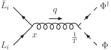
Figure 4: Weak isospin boson exchange that generates the fermion-Higgs operator.

For completeness we also give the matching coefficient $c_{3,i}$ for the fermion-Higgs operator $(\bar{L}_{i}\gamma^{\mu}\tau^{a}L_{i})(\Phi^{\dagger}\overleftrightarrow{i\tau^{a}D_{\mu}}\Phi)$, which gives rise to diagram (d1) in figure 1. Only SU(2) gauge-boson exchange shown in figure 4 can generate an operator with a single charged scalar at tree level. The fifth component of the 5D gauge boson cannot contribute due to the boundary conditions. We find

$$c_{3,i}=-i\,\frac{(ig_{5})^{2}}{2}T^{2}\int_{1/k}^{1/T}dx\,\frac{{f_{L_{i}}^{(0)}}^{2}\!(x)}{(kx)^{4}}\Delta_{\perp}^{ZMS}(q=0,x,1/T)\,.$$ (37)

Inserting (29) into (37) we obtain

$$c_{3,i}= -\frac{g^{2}}{8}T^{2}\,\Bigg{(}\frac{1/T^{2}-1/k^{2}}{\ln\frac{k}{T}}-\frac{1}{T^{2}}+\int_{1/k}^{1/T}dx\,\frac{{f_{L_{i}}^{(0)}}^{2}\!(x)}{(kx)^{4}}\,x^{2}\big{(}2\ln(kx)-1\big{)}\Bigg{)}.$$ (38)

As above, we neglect $1/k^{2}$ relative to $1/T^{2}$, and keep only the leading term in $\epsilon$. Using the normalization of the fermion modes simplifies the expression to

$$c_{3,i}=\frac{g^{2}}{8}\,\Bigg{(}1-\frac{1}{\ln 1/\epsilon}-\left[\frac{(1-2c_{L_{i}})(5-2c_{L_{i}})}{(3-2c_{L_{i}})^{2}}-\frac{2(1-2c_{L_{i}})\ln 1/\epsilon}{(3-2c_{L_{i}})}\right]\frac{\epsilon^{2c_{L_{i}}-1}}{1-\epsilon^{2c_{L_{i}}-1}}\Bigg{)}.$$ (39)

Note that $c_{3,i}$ is about $10^{2}$ times larger than $b_{ij}$, since it is proportional to the SU(2) gauge coupling and since its largest term does not feature the suppression factor $\frac{1}{\ln 1/\epsilon}\sim 1/35$ that is present in $b_{ij}$. For $c_{L_{i}}$ larger than but not too close to $1/2$ the dependence of $c_{3,i}$ on the model parameters is rather mild, since the 1 in the round brackets dominates.

3.3 Electromagnetic dipole operator

The matching coefficient of the electromagnetic dipole operator is more difficult to compute, since it comes from the 5D one-loop diagrams in figure 2. We are interested only in the electromagnetic dipole transition, so we take the external gauge boson to be the superposition $c_{W}B^{\mu}+s_{W}W^{3,\mu}$ corresponding to the photon. We also anticipate that the Higgs doublet $\Phi$ in the operators $\bar{L}_{i}\Phi\sigma_{\mu\nu}E_{j}B^{\mu\nu}$ and $\bar{L}_{i}\tau^{a}\Phi\sigma_{\mu\nu}E_{j}\,W^{a,\mu\nu}$ will be replaced by its vacuum expectation value and therefore extract only the weak isospin component that corresponds to charged lepton $\ell_{i}\to\ell_{j}\gamma$ transitions after electroweak symmetry breaking. These simplifications have already been employed to omit some additional diagrams with the photon coupling to the Higgs-doublet field. To compute the matching coefficient we apply the following strategy:

• Subtract the zero mode from every internal 5D gauge boson propagator. It can be shown that selecting the gauge-boson zero modes forces the fermion propagators to only propagate zero modes. This follows from the flatness of the gauge boson and orthogonality of the fermion mode functions. Thus, the subtracted terms correspond precisely to the Standard Model contribution to $(g-2)_{\mu}$.

• Expand the diagram in the external fermion momenta $p$, $p^{\prime}$ and neglect the (tachyonic) mass in the SU(2) Higgs propagator. This ensures that we pick up only the contribution from loop momenta $l\sim T$ as appropriate for a matching coefficient. Some of the one-loop diagrams have tree-level subgraphs corresponding to propagating KK excitations while the loop momentum is of order of the electroweak or muon mass scale. These contributions are excluded by the above expansion; they have already been accounted for by the other dimension-6 operators with coefficient functions $b$, $c_{i}$ and the one-loop diagrams in Sec. 2.3 as discussed above.

3.3.1 Sample diagram

We now illustrate this procedure by discussing the calculation of diagram B1a from figure 2 in further detail. With the 5D Feynman rules from appendix A we find for this diagram the expression

$${\rm{\bf B1a}} = (ig^{\prime}_{5})^{2}(ie_{5}Q_{\mu})\left(\frac{-iT^{3}}{k^{3}}\right)y^{\rm(5D)}_{ij}\,\frac{Y_{L}}{2}\frac{Y_{E}}{2}\int^{1/T}_{1/k}\!\!\!\frac{dx}{(kx)^{4}}\int^{1/T}_{1/k}\!\!\!\frac{dy}{(ky)^{4}}\int^{1/T}_{1/k}\!\!\!\frac{dz}{(kz)^{4}}\int\!\frac{d^{4}l}{(2\pi)^{4}}$$ (40)

$$f^{(0)}_{L_{i}}(z)f^{(0)}_{\gamma}(y)g^{(0)}_{E_{j}}(x)\,\epsilon^{*\mu}\Delta^{\rho\nu}_{\mbox{\tiny ZMS}}(l,x,z)$$

$$\bar{L_{i}}(p^{\prime})P_{R}\gamma_{\rho}\Delta^{L}_{i}({p^{\prime}-l},z,y)\gamma_{\mu}\Delta^{L}_{i}({p-l},y,1/T)\Delta^{E}_{j}({p-l},1/T,x)\gamma_{\nu}P_{R}E_{j}(p),\qquad$$

which contains the 5D propagators of the fermions and the zero-mode subtracted hypercharge gauge boson, and the wave functions $f^{(0)}_{L_{i}}(z)\bar{L_{i}}(p^{\prime})$, $g^{(0)}_{E_{j}}(x)E_{j}(p)$, $f^{(0)}_{\gamma}(y)\epsilon^{*\mu}$ of the external states, which are the zero modes of the 5D fields. The positions of the three vertices in the 5th dimension, $x$, $y$, $z$, and the four-dimensional loop momentum $l$ are integrated over. The electromagnetic charge prefactor arises, because the coupling of the external photon in isospin space is $[\frac{Y_{L}}{2}\mathds{1}+\frac{\tau^{3}}{2}]_{22}=Q_{\mu}=-1$.

We decompose each fermion propagator into its four chiral components using (A.3.1). Most of the 64 possible terms vanish due to the projectors $P_{R}$ in (40) and the brane boundary conditions $g_{L_{i}}(1/T)=f_{E_{j}}(1/T)=0$, see (101), (102). The two remaining terms can be deduced from (142a), which results in

$${\rm{\bf B1a}} = \frac{g^{\prime 2}_{5}e_{5}Q_{\mu}Y_{L}Y_{E}y^{\rm(5D)}_{{ij}}T^{3}}{4k^{3}}\int^{1/T}_{1/k}\!\!\!\frac{dx}{(kx)^{4}}\int^{1/T}_{1/k}\!\!\!\frac{dy}{(ky)^{4}}\int^{1/T}_{1/k}\!\!\!\frac{dz}{(kz)^{4}}\int\!\!\!\frac{d^{4}l}{(2\pi)^{4}}$$ (41)

$$f^{(0)}_{L_{i}}(z)f^{(0)}_{\gamma}(y)g^{(0)}_{E_{j}}(x)\epsilon^{*\mu}\Delta^{\rho\nu}_{\mbox{\tiny ZMS}}(l,x,z)$$

$$\bar{L_{i}}(p^{\prime})\Big{[}F^{+}_{L_{i}}({\hat{p}^{\,\prime}},z,y)F^{+}_{L_{i}}({\hat{p}},y,1/T)F^{-}_{E_{j}}({\hat{p}},1/T,x)\left\{\gamma_{\rho}(\not\!p^{\,\prime}-\!\!\!\not l)\gamma_{\mu}\gamma_{\nu}\right\}(p-l)^{2}+$$

$$d^{+}F^{-}_{L_{i}}({\hat{p}^{\,\prime}},z,y)d^{-}F^{+}_{L_{i}}({\hat{p}},y,1/T)F^{-}_{E_{j}}({\hat{p}},1/T,x)\left\{\gamma_{\rho}\gamma_{\mu}(\not\!p-\!\!\!\not l)\gamma_{\nu}\right\}\Big{]}P_{R}E_{{j}}(p),$$

where $\hat{p}=p-l$, $\hat{p}^{\,\prime}=p^{\prime}-l$. In the KK picture the first term in square brackets corresponds to picking up three momentum factors from the propagator numerators, while the second contains two KK mass factors. In appendix C we provide the expressions corresponding to (40), (41) for all 21 one-particle irreducible diagrams shown in figure 2.

We note that at this point the integral over the coordinate $y$ of the external photon vertex could be performed analytically. Since the photon zero mode is constant and combines with $e_{5}f^{(0)}_{\gamma}(y)=e$ to the dimensionless 4D electric charge, the remaining $y$-integral is

$$\int^{1/T}_{1/k}\!\!\!\frac{dy}{(ky)^{4}}\,F^{+}_{L_{i}}({\hat{p}^{\,\prime}},z,y)F^{+}_{L_{i}}({\hat{p}},y,1/T)=\sum_{n}\frac{(-i)^{2}f_{L_{i}}^{(n)}(z)f_{L_{i}}^{(n)}(1/T)}{({\hat{p}^{\,\prime}}{}^{2}-m_{n}^{2})({\hat{p}}^{2}-m_{n}^{2})}$$ (42)

and a similar expression for the mass terms. The key point is that the $y$-integral is the orthogonality relation of the fermion mode functions. Thus, the KK number is not changed at the external photon vertex and the remaining sum involves only two mode functions. The KK sum can be expressed in terms of Bessel functions. However, the result is algebraically complicated, so we do not make use of this simplification in the numerical evaluation of the diagrams.

Returning to (41) we perform the expansion in the small external momenta $p$, $p^{\prime}$ and pick up the terms linear in the momenta, since these produce the electromagnetic dipole structure $i\sigma^{\mu\nu}q_{\nu}$ after application of the Gordon identity. Since the various $F$-functions depend only on the square of the four-momentum argument, this expansion can be done by using, e.g.,

$$F^{+}_{L_{i}}(p^{\,\prime}-l,z,y)=F^{+}_{L_{i}}(l,z,y)-2p^{\prime}\cdot l\,\frac{\partial}{\partial l^{2}}F^{+}_{L_{i}}(l,z,y)+\ldots.$$ (43)

The derivatives of all required propagator functions are listed in appendix B. In Feynman gauge (where the gauge boson propagator is proportional to $\eta^{\rho\nu}$), the first term in square brackets in (41) turns into

$$F^{+}_{L_{i}}(l,z,y)F^{+}_{L_{i}}(l,y,1/T)F^{-}_{E_{j}}(l,1/T,x)\left\{\gamma^{\nu}\!\!\not\!p^{\,\prime}\gamma_{\mu}\gamma_{\nu}\,l^{2}+\gamma^{\nu}\!\!\!\not l\gamma_{\mu}\gamma_{\nu}\,2p\cdot l\right\}$$

$$+\,\gamma^{\nu}(-\!\!\!\not l)\gamma_{\mu}\gamma_{\nu}\,l^{2}\,\bigg{\{}-2p^{\prime}\cdot l\left(\frac{\partial}{\partial l^{2}}F^{+}_{L_{i}}(l,z,y)\right)F^{+}_{L_{i}}(l,y,1/T)F^{-}_{E_{j}}(l,1/T,x)$$

$$\hskip 28.45274pt-\,2p\cdot l\,F^{+}_{L_{i}}(l,z,y)\,\frac{\partial}{\partial l^{2}}\left[F^{+}_{L_{i}}(l,y,1/T)F^{-}_{E_{j}}(l,1/T,x)\right]\bigg{\}}\,,$$ (44)

where terms odd in the loop momentum $l$ have already been dropped, since they integrate to zero. The angular integrations can now be done trivially. In the above integral we simply replace $l^{\alpha}l^{\beta}\to\eta^{\alpha\beta}\,l^{2}/4$ and perform the Dirac algebra. Employing the on-shell conditions,

$$\gamma^{\nu}\!\!\not\!p^{\,\prime}\gamma_{\mu}\gamma_{\nu}\to 4p^{\,\prime}_{\mu},\qquad\gamma^{\nu}\!\!\!\not l\gamma_{\mu}\gamma_{\nu}\,2p\cdot l\to 2p_{\mu}\,l^{2}$$ (45)

etc. What remains is a scalar integrand that depends on $l^{2}$ only, and the bulk coordinates $x,y,z$. The integral can be evaluated numerically after performing the Wick rotation $l^{2}\to-l^{2}$. The propagators given explicitly in the appendix refer to these Wick-rotated (“Euclidean”) propagators. Diagrams involving internal Higgs lines are easier to evaluate, since the number of independent bulk coordinates to be integrated reduces to two or even one, due to the brane localization of the Higgs field.

For the numerical evaluation the loop integral needs to be ultraviolet and infrared finite. We find that the integration converges for large $l$, as expected since the leading one-loop expression for the anomalous magnetic moment should not require UV renormalization. The diagrams are also IR finite with the exception of the internal insertion diagrams B1a and B1b, for which only the sum is finite, and the non-abelian diagram W8. The IR divergence arises when all internal fermion modes are zero modes. There is no IR divergence in the internal insertion diagrams B3a, B3b with scalar hypercharge boson exchange, since the chirality-flip at the fermion-$B_{5}$ vertex forbids the propagation of zero modes in these diagrams. The existence of an IR divergence in B1a, B1b and W8 implies that the purely four-dimensional treatment described above potentially misses terms of the form $1/\epsilon\times\epsilon$. We discuss this further below.

3.3.2 External insertions

Another comment is necessary on the diagrams with an external Higgs insertion, such as B2a. The fermion propagator that connects the external Higgs vertex to the internal gauge vertex is (in this example)

$$\Delta_{i}^{L}(p,x,1/T)P_{R}=-F_{L_{i}}^{+}(p,x,1/T)p\hskip-4.49997pt/P_{R}+d^{-}F_{L_{i}}^{+}(p,x,1/T)P_{R}\,.$$ (46)

If this expression contained a relevant $1/p^{2}$ contribution from the zero mode, the diagram would be long-distance sensitive, and the expansion in the small external momenta would be invalid. The second term is a mass term, see (142a), to which the zero mode cannot contribute, since $m_{0}=0$. Hence this term can be expanded in $p$, and since it depends only on $p^{2}$, we can simply set $p=0$ to linear order. The zero mode is present in the first term, which contains $ip\hskip-4.49997pt//p^{2}\times f_{L_{i}}^{(0)}(x)f_{L_{i}}^{(0)}(1/T)$. If the one-particle pole at $p^{2}=0$ remains in the final answer, then this part of the external Higgs insertion into a zero mode needs to be amputated; it corresponds to the first term in the sum of tree diagrams that sums to the SM lepton mass matrix. After amputation the remaining short-distance contribution is a one-loop correction to the chirality preserving $\bar{L}_{i}L_{i}\gamma$ vertex. The general $\bar{L}_{i}L_{i}\gamma$ vertex function with off-shell zero-mode fermions can be decomposed into “on-shell” and “off-shell” terms as follows:

$$\Lambda^{\mu}=\Lambda^{\mu}_{\rm on}+p\hskip-4.49997pt/^{\prime}\Lambda^{\mu}_{\rm off,\,p^{\prime}}+\Lambda^{\mu}_{\rm off,\,p}\,p\hskip-4.49997pt/\,.$$ (47)

The first piece constitutes the correction to the on-shell $\bar{L}_{i}L_{i}\gamma$ vertex and is not relevant to the anomalous magnetic moment. It constitutes the long-distance piece that must be amputated. The off-shell term with a $p\hskip-4.49997pt/^{\prime}$ vanishes, since diagram B2a has an on-shell external $p^{\prime}$ line on the right. However, the $\Lambda^{\mu}_{\rm off,\,p}\,p\hskip-4.49997pt/$ term cancels the propagator factor $p\hskip-4.49997pt//p^{2}$ from the internal fermion line, and represents a short-distance contribution that must be added to the matching coefficient of the dipole operator and hence contributes to $(g-2)_{\mu}$.

It follows that in all external insertion diagrams we have two different contributions to consider. The first one can be obtained by replacing

$$\Delta_{i}^{L}(p,x,1/T)\to d^{-}F_{L_{i}}^{+}(p=0,x,1/T)=\sum_{n\not=0}\frac{-i}{m_{n}}g_{L_{i}}^{(n)}(x)f_{L_{i}}^{(n)}(1/T)$$

$$\hskip 28.45274pt=-i\,\frac{k^{4}x^{5/2}}{T^{3/2}}\,\frac{(kx)^{1/2-c_{L_{i}}}-(kx)^{c_{L_{i}}-1/2}}{\left(\frac{T}{k}\right)^{\!c_{L_{i}}-1/2}-\left(\frac{k}{T}\right)^{\!c_{L_{i}}-1/2}},$$ (48)

where the last expression follows from the explicit expression for the propagator functions given in the appendix. We note that the KK mode contribution to $d^{-}F_{L_{i}}^{+}(p,x,1/T)$ is not suppressed due to the large KK masses of order $T$. Thus, the external insertion diagrams are not suppressed relative to the internal insertions, contrary to what has been assumed in the previous literature, where the external insertions have been neglected.

The second contribution stems from the off-shell vertex terms and explicitly contains the zero-mode propagator. It can be obtained via the replacement

$$\Lambda^{\mu}\Delta_{i}^{L}(p,x,1/T)\to\Lambda^{\mu}_{\rm off,\,p}\,p\hskip-4.49997pt/\times ip\hskip-4.49997pt//p^{2}\times f_{L_{i}}^{(0)}(x)f_{L_{i}}^{(0)}(1/T)=i\,\Lambda^{\mu}_{\rm off,\,p}\,f_{L_{i}}^{(0)}(x)f_{L_{i}}^{(0)}(1/T)\,,\qquad$$ (49)

where the internal zero-mode pole is cancelled. We will refer to these second contributions as “off-shell” terms. They require the separate computation of the $\Lambda^{\mu}_{\rm off,\,p}$ structure of the $\bar{L}_{i}L_{i}\gamma$ vertex, which can be obtained from the expansion in the small external momenta. The expansion must now be performed to second order, since we need the $p\hskip-4.49997pt/p^{\mu}$, $p\hskip-4.49997pt/p^{\prime\mu}$ structures in the vertex function $\Lambda^{\mu}$.

The second contribution appears to be suppressed by a power of the lepton mass matrix due to the two additional fermion zero mode profiles. The expansion of $\Lambda^{\mu}$ to second order brings an additional factor $1/T$ from the scale of the loop momentum. The ratio of the second to the first contribution can therefore be estimated as

$$\frac{\frac{i}{T}f_{L_{i}}^{(0)}(x)f_{L_{i}}^{(0)}(1/T)}{d^{-}F_{L_{i}}^{+}(p=0,x,1/T)}\approx-\left[\sqrt{\frac{1-2c_{L_{i}}}{1-(T/k)^{1-2c_{L_{i}}}}}\,\right]^{2}\,,$$ (50)

where we put $x=1/T$ for the second estimate. For symmetric bulk mass parameters $c_{E_{i}}=-c_{L_{i}}$ such that $f_{L_{i}}^{(0)}(x)=g_{E_{i}}^{(0)}(x)$, and anarchic Yukawa couplings this is indeed of order $m_{\ell_{i}}/v$, see (13). For the other special choice $c_{L}\to 0.5$ we find

$$\frac{\frac{i}{T}f^{(0)}_{L_{i}}(x)f^{(0)}_{L_{i}}(1/T)}{d^{-}F^{+}_{L_{i}}(p=0,x,1/T)}\to-\frac{1}{Tx\log(kx)}\;.$$ (51)

For $x$ close to $1/T$ this approaches $-1/\log(1/\epsilon)\approx-1/35$, and we obtain a lepton-mass independent suppression. Thus, the “off-shell” terms are expected to be subleading for standard choices of the bulk mass parameters, which is indeed found in the exact numerical evaluation discussed in Sec. 4.1.

3.3.3 Scheme independence

We mentioned above that the naive four-dimensional calculation of the sum of the individually IR divergent diagrams B1a+B1b might be wrong, since it could miss terms of the form $1/\varepsilon\times\varepsilon$. A similar issue appears in the finite result (21) for diagram (b) from figure 1, for which we would obtain zero, if the Dirac algebra were performed naively in four dimensions. The finite results of both calculations depend on the treatment of $\gamma_{5}$ in $d$ dimensions. In the following we show algebraically that the scheme dependence cancels if the same scheme is applied consistently to both parts, and that the finite result agrees with what we obtained above.

Both parts are limits of a diagram in the full 5D theory with fields expanded around the electroweak vacuum and massive zero-mode fermions. This diagram is finite (as far as the $\sigma^{\mu\nu}q_{\nu}$ structure is concerned). The divergences arise only when this diagram is split into a short-distance contribution from the KK scale, diagrams B1a+B1b, and a long-distance contribution from the electroweak and lepton mass scale, represented by the four-fermion operator insertion diagram. Before factorizing the full-theory diagram we can freely anti-commute $\gamma_{5}$. The convention that corresponds to (21) amounts to eliminating all chiral projectors except for two placed at the operator vertex $\gamma^{\rho}P_{L}\otimes\gamma_{\rho}P_{R}$.

For consistency, the same convention must be applied to the starting expression for the diagrams B1a+B1b, which therefore reads

$$\Gamma^{\mu}(p,p^{\prime}) = (ieQ_{\mu})(ig^{\prime}_{5})^{2}\left(\frac{-iT^{3}}{k^{3}}\right)\frac{v}{\sqrt{2}}\,[U^{\dagger}]_{2m}y^{\rm(5D)}_{mn}V_{n2}~{}\frac{Y_{L}}{2}\frac{Y_{E}}{2}\,f^{(0)}_{L_{m}}(1/T)g^{(0)}_{E_{n}}(1/T)$$ (52)

$$\int^{1/T}_{1/k}\!\!dxdz\,\frac{{f_{L_{m}}^{(0)}}^{2}\!(x)}{(kx)^{4}}\,\frac{{g_{E_{n}}^{(0)}}^{2}\!(z)}{(kz)^{4}}\,\,\mu^{2\varepsilon}\int\!\!\frac{d^{d}l}{(2\pi)^{d}}\,\Delta^{\rho\nu}_{\mbox{\tiny ZMS}}(l,x,z)$$

$$i^{3}\,\bar{L}_{m}(p^{\prime})\gamma_{\rho}P_{L}\frac{p\hskip-4.49997pt/^{\,\prime}-l\hskip-4.49997pt/}{(p^{\prime}-l)^{2}}\left[\gamma^{\mu}\frac{p\hskip-4.49997pt/-l\hskip-4.49997pt/}{(p-l)^{2}}+\frac{p\hskip-4.49997pt/^{\,\prime}-l\hskip-4.49997pt/}{(p^{\prime}-l)^{2}}\gamma^{\mu}\right]\frac{p\hskip-4.49997pt/-l\hskip-4.49997pt/}{(p-l)^{2}}\gamma_{\nu}P_{R}E_{n}(p)\,.\qquad$$

To obtain this result, we write down the explicit expressions from appendix C and multiply it by $[U^{\dagger}]_{2i}V_{j2}$ so that the external states correspond to the SM muons in the mass eigenbasis. All fermion propagators can be replaced by zero-mode propagators, since only this term is IR divergent, and the chiral projectors are placed as discussed above. Performing the integration over the bulk coordinate $y$ of the photon vertex, we arrive at (52).

The IR divergence comes from $l\ll T$, hence we can set $l=0$ in the zero-mode subtracted gauge-boson propagator. Moreover, only the $\eta^{\rho\nu}$ structure contributes to the IR divergence. After these simplifications, we can identify the expression (28) for $b_{ij}$. We perform the expansion in external momenta and simplify the Dirac algebra as much as possible. When the Dirac structure is multiplied by a $1/\varepsilon$ pole we do not anti-commute $\gamma_{5}$ with $\gamma_{\alpha}$, but since the external momenta are four-dimensional we may use that $p\hskip-4.49997pt/^{(\prime)}\gamma_{5}=-\gamma_{5}\,p\hskip-4.49997pt/^{(\prime)}$. The result of all this is that the IR sensitive contribution in the matching coefficient of the electromagnetic dipole operator is given by

$$\Gamma^{\mu}_{\mbox{\scriptsize IR}}(p,p^{\prime}) = ieQ_{\mu}\frac{m_{l_{k}}\beta_{2kk2}}{16\pi^{2}T^{2}}\,\bar{u}(p^{\prime},s^{\prime})\Big{[}2\,(p+p^{\prime})^{\mu}P_{R}-\frac{1}{\varepsilon}\,\gamma^{\rho}P_{L}i\sigma^{\mu\nu}q_{\nu}\gamma_{\rho}P_{R}\Big{]}u(p,s).\quad$$ (53)

The second term in brackets cannot be further reduced without assumptions on $\gamma_{5}$. Since $\gamma^{\rho}P_{L}i\sigma^{\mu\nu}q_{\nu}\gamma_{\rho}P_{R}$ vanishes in four dimensions, the entire expression is finite, but scheme-dependent.

In the one-loop matrix element calculation of the four-fermion operator that led to (21) we assumed the naive dimensional regularization (NDR) scheme to obtain the result in the last line. We repeat the calculation in an arbitrary scheme, leaving out the $(\beta_{2kk2}\leftrightarrow\beta_{k22k},\,P_{L}\leftrightarrow P_{R})$ term, which is related to the matching coefficient of the electromagnetic dipole operator with $L$ and $E$ exchanged. It is easy to see that the ultraviolet $1/\varepsilon$ pole in the one-loop matrix element (21) that is relevant to the electromagnetic dipole transition is obtained correctly by approximating $(l\hskip-4.49997pt/+m_{\ell_{k}})\gamma^{\mu}(l\hskip-4.49997pt/-q\hskip-4.49997pt/+m_{\ell_{k}})\to-m_{\ell_{k}}\gamma^{\mu}q\hskip-4.49997pt/$. Dropping terms proportional to $q^{\mu}$, we obtain

$$\Gamma^{\mu}_{\mbox{\scriptsize UV}}(p,p^{\prime}) = ieQ_{\mu}\frac{m_{l_{k}}\beta_{2kk2}}{16\pi^{2}T^{2}}\,\frac{1}{\varepsilon}\,\bar{u}(p^{\prime},s^{\prime})\Big{[}\gamma^{\rho}P_{L}i\sigma^{\mu\nu}q_{\nu}\gamma_{\rho}P_{R}\Big{]}u(p,s).$$ (54)

Now we can make the following two observations:

• In the NDR scheme (anti-commuting $\gamma_{5}$), between $\bar{u}(p^{\prime},s^{\prime})[\ldots]u(p,s)$,

  $$\gamma^{\rho}P_{L}i\sigma^{\mu\nu}q_{\nu}\gamma_{\rho}P_{R}=2\varepsilon\,(p+p^{\prime})^{\mu}P_{R}=-2\varepsilon\,i\sigma^{\mu\nu}q_{\nu}P_{R}\,,$$ (55)

  where the Gordon identity is used in the last step, and the term not related to the electromagnetic dipole structure is dropped. Then (53) is zero and (54) coincides with (21). Thus we reproduce the previous results.

• In an arbitrary scheme the scheme-dependent terms drop out when summing $\Gamma^{\mu}_{\mbox{\scriptsize IR}}(p,p^{\prime})$ and $\Gamma^{\mu}_{\mbox{\scriptsize UV}}(p,p^{\prime})$, and the result agrees with the one obtained before in the NDR scheme.

This proves that the result is scheme-independent, and that the naive four-dimensional treatment of diagrams B1a, B1b fortuitously gives the correct result.

A similar issue arises for the IR-sensitive diagram W8, but in this case it turns out that the naive four-dimensional calculation needs to be corrected by a finite term of the form $1/\varepsilon\times\varepsilon$ that is present when working consistently in $4-2\varepsilon$ dimensions. This finite term is scheme-dependent in general, and the scheme-dependence is compensated by the effective theory diagram (d1) in figure 1. The zero result (24) for diagram (d1) corresponds to a full-theory diagram in which the charged-Higgs vertex in (16) is written as $\bar{\psi}_{i}P_{R}\gamma_{\mu}\nu_{j}$ rather than $\bar{\psi}_{i}\gamma_{\mu}P_{L}\nu_{j}$. We must apply this convention consistently to diagram W8 as well. The IR sensitive part of W8 can be obtained from (182) by replacing the internal fermion by the zero mode. Then, rotating the external states to the mass eigenbasis by multiplying (182) by $[U^{\dagger}]_{2i}V_{j2}$, the relevant part of W8 simplifies to

$$\Gamma^{\mu}(p,p^{\prime})= (ig_{5})^{2}(ie_{5})\left(\frac{\tau^{a}}{2}\left[\frac{Y_{\Phi}}{2}+\frac{\tau^{3}}{2}\right]\frac{\tau^{a}}{2}\right)_{\!\!22}\left(\frac{-iT^{3}}{k^{3}}\right)\frac{[U^{\dagger}]_{2i}vy^{\rm(5D)}_{ij}V_{j2}}{\sqrt{2}}f^{(0)}_{L_{i}}(1/T)g^{(0)}_{E_{j}}(1/T)$$

$$\times\mu^{2\varepsilon}\int\!\!\frac{d^{d}l}{(2\pi)^{d}}\,\int^{1/T}_{1/k}\!\!dx\,\frac{{f_{L_{i}}^{(0)}}^{2}(x)}{(kx)^{4}}\Delta^{\rho\nu}_{\mbox{\tiny ZMS}}(p^{\prime}-l,x,1/T)f^{(0)}_{\gamma}(1/T)$$

$$\times i^{3}\,\bar{L}(p^{\prime})P_{R}\frac{(p^{\prime}-l)_{\nu}\gamma_{\rho}\not{l}(p+p^{\prime}-2l)^{\mu}}{(p-l)^{2}(p^{\prime}-l)^{2}l^{2}}P_{R}E(p)\,.$$ (56)

Exploiting $q_{\nu}\,\Delta^{\rho\nu}_{\mbox{\tiny ZMS}}(q,x,1/T)=q_{\rho}\,\Delta_{\parallel}^{\mbox{\tiny ZMS}}(q,x,1/T,\xi)$ , which follows from (150),

$$\frac{T^{3}}{k^{3}}\frac{y^{\rm(5D)}_{ij}v}{\sqrt{2}}f^{(0)}_{L_{i}}(1/T)g^{(0)}_{E_{j}}(1/T)=\sum_{k}m_{k}\;U_{ik}\mathds{1}_{kh}V^{\dagger}_{hj}\,,$$ (57)

and $e_{5}f^{(0)}_{\gamma}(x)=e$, this simplifies further to

$$\Gamma^{\mu}(p,p^{\prime}) = g_{5}^{2}(ie)\,\frac{1}{2}\,m_{\mu}\sum_{i}\,[U^{\dagger}]_{2i}U_{i2}\,\mu^{2\varepsilon}\int\!\!\frac{d^{d}l}{(2\pi)^{d}}\,\int^{1/T}_{1/k}\!\!dx\,\frac{{f_{L_{i}}^{(0)}}^{2}(x)}{(kx)^{4}}\Delta_{\parallel}^{\mbox{\tiny ZMS}}(p^{\prime}-l,x,1/T,\xi)$$ (58)

$$\times\bar{L}(p^{\prime})P_{R}\frac{(\not{p}^{\prime}-\not{l})\not{l}(p+p^{\prime}-2l)^{\mu}}{(p-l)^{2}(p^{\prime}-l)^{2}l^{2}}P_{R}E(p)\,.$$

Since the difference to the naive four-dimensional calculation arises only from $l\ll T$, we apply a cut-off $l\ll\Lambda\ll T$ to the loop momentum. This allows us to set the gauge-boson propagator momentum to zero without generating a spurious UV divergence, and to identify the coefficient function $c_{3,i}$, since $\Delta_{\parallel}^{\mbox{\tiny ZMS}}(0,x,1/T,\xi)=\Delta^{\mbox{\tiny ZMS}}_{\perp}(0,x,1/T)$. Expansion to linear order in $p$, $p^{\prime}$ results in

$$\Gamma^{\mu}(p,p^{\prime}) = (-e)\,\frac{m_{\mu}}{T^{2}}\sum_{i}\,c_{3,i}[U^{\dagger}]_{2i}U_{i2}\,\mu^{2\varepsilon}\int\limits^{\Lambda}\!\!\frac{d^{d}l}{(2\pi)^{d}}\,\frac{1}{l^{4}}\left[(p+p^{\prime})^{\mu}-\frac{4l^{\mu}(p+p^{\prime})\cdot l}{l^{2}}\right]$$ (59)

$$\times\bar{L}(p^{\prime})P_{R}E(p)\,.$$

The difference between the correct and naive treatment comes from the second term in square brackets, where we must use $l^{\mu}l^{\nu}\to 1/d\times l^{2}\eta_{\mu\nu}$ instead of $1/4$ as done in the four-dimensional treatment of the integrand. Using the definition (17) of $\gamma_{3,ij}$, we therefore find that the difference between the $d$-dimensional and four-dimensional result that must be added to the naive four-dimensional treatment of W8 is

$$\Delta\Gamma^{\mu}(p,p^{\prime}) = (-e)\,\frac{\gamma_{3,22}m_{\mu}}{T^{2}}\,\left(-\frac{4}{d}+1\right)\,\mu^{2\varepsilon}\int\limits^{\Lambda}\!\!\frac{d^{d}l}{(2\pi)^{d}}\,\frac{1}{l^{4}}\times\bar{L}(p^{\prime})P_{R}(p+p^{\prime})^{\mu}E(p)$$ (60)

$$= ieQ_{\mu}\,\frac{\gamma_{3,22}m_{\mu}}{32\pi^{2}T^{2}}\,\times\bar{L}(p^{\prime})P_{R}(p+p^{\prime})^{\mu}E(p)+{\cal O}(\varepsilon)\,.$$

The result is independent of the arbitrary cut-off as it should be and is part of $a_{W,ij}$, the coefficient of the class-0 operator $\bar{L}_{i}\tau^{a}\Phi\sigma_{\mu\nu}E_{j}\,W^{a,\mu\nu}$. We can check (60) by noting that it should be minus the UV sensitive $\varepsilon\times 1/\varepsilon$ term in the matrix element calculation that led to (26). Since $Q_{\mu}=-1$ this is indeed the case.

In principle the issue of scheme-dependence could also occur for diagrams B5a, B5b and W3, related to the effective theory diagrams (c1), (c2). However, it can be checked that in this case our convention for the position of the chiral projection operators in (16) implies that diagrams (c1) and (c2) are always zero and accordingly there are no $\varepsilon\times 1/\varepsilon$ terms in B5a, B5b and W3.

3.3.4 Gauge invariance

To check the gauge independence of the matching coefficient, we performed the calculation in 5D $R_{\xi}$ gauge, and verified that our numerical result is independent of $\xi$ for a range of values of $\xi$. We also checked analytically that the $\xi$-dependent terms cancel. The proof is too lengthy to be presented here explicitly, but we find it instructive to discuss the structure of the argument and the key algebraic identities.

It is clear that the subsets of diagrams with hypercharge and SU(2) gauge boson exchange must be separately gauge-independent. It is also evident that the five diagrams Bxa and the other five hypercharge exchange diagrams Bxb must be separately invariant, since the dependence on the bulk mass parameters $c_{L_{i}}$ and $c_{E_{j}}$ is different whether the Higgs coupling to the fermion is to the left or to the right of the one of the external photon. Hence we consider first B1a to B5a, see figure 2.

The gauge-parameter dependence arises from the scalar gauge boson propagator $\Delta_{5}$ (see (153), (157)) and the longitudinal part

$$\frac{l^{\rho}l^{\nu}}{l^{2}}\,\Delta_{\parallel}(l,z,z^{\prime},\xi)=\frac{l^{\rho}l^{\nu}}{l^{2}}\,\Delta_{\perp}(l/\sqrt{\xi},z,z^{\prime})$$ (61)

of the vector gauge boson propagator. In diagrams B1a, B2a and B5a we therefore replace $\Delta^{\rho\nu}(l,z,z^{\prime})$ by the previous expression. Using (119), the mode representation of the propagator, and the completeness relation $\sum_{n}f_{B_{5}}^{(n)}(z)f_{B_{5}}^{(n)}(z^{\prime})=kz\,\delta(z-z^{\prime})$ we derive the identity

$$\Delta_{5}(l,z,z^{\prime})=\frac{ikz}{l^{2}}\,\delta(z-z^{\prime})-\frac{1}{l^{2}}\,\partial_{z}\partial_{z^{\prime}}\Delta_{\perp}(l/\sqrt{\xi},z,z^{\prime}),$$ (62)

which is used to eliminate the propagator of the scalar component of the gauge boson in diagrams B3a and B4a. At this point all gauge-dependence is in the expression $\Delta_{\perp}(l/\sqrt{\xi},z,z^{\prime})$, which appears in all five diagrams. The delta-function term in (62) results in a $\xi$-independent expression that can be ignored.

To proceed we need an identity that relates the different diagram topologies – internal insertions (B1a, B3a), external insertions (B2a, B4a), and Higgs (B5a) diagrams. This is obtained as follows. After using (62), we integrate by parts the bulk coordinate derivatives on $\Delta_{\perp}$, which yields the corresponding derivatives on the two fermion propagators (B3a), or one propagator and one external zero mode (B4a) adjacent to the gauge boson vertex. Now we can use successively identities such as

$$\partial_{z}\left(\frac{1}{(kz)^{4}}\,\Delta_{i}^{L}(p_{1},x,z)\gamma_{5}\Delta_{i}^{L}(p_{2},z,y)\right)=\frac{1}{(kz)^{4}}\,\Delta_{i}^{L}(p_{1},x,z)\left(p\hskip-4.49997pt/_{1}-p\hskip-4.49997pt/_{2}\right)\Delta_{i}^{L}(p_{2},z,y)$$

$$\hskip 28.45274pt+\,i\Delta_{i}^{L}(p_{1},x,z)\delta(z-y)-i\Delta_{i}^{L}(p_{2},z,y)\delta(x-z)$$ (63)

which follow from the defining equations for the fermion propagator (121), (122). If one of the propagators on the left-hand side of (63) is an external zero mode, the corresponding delta-function and momentum term is absent. When this is used in B3a and B4a, the first term on the right-hand side of (63) cancels precisely the gauge-dependent terms of B1a and B2a, respectively, leaving over only the delta-function terms and the Higgs diagram B5a.

Some of the delta-function terms vanish, since the remaining integral is independent of $p^{\prime}$ ($p$), such that the loop integral must result in $p\hskip-4.49997pt/E(p)_{j}=0$ ($\bar{L}_{i}(p^{\prime})p\hskip-4.49997pt/^{\prime}=0$). The surviving two terms correspond to diagrams with one deleted propagator. Inspection shows that these two terms and the Higgs diagram B5a are identical up to a different hypercharge prefactor. The prefactors are such that we obtain

$$Y_{L}\,\mbox{[B3a]}-Y_{E}\,\mbox{[B4a]}-Y_{\phi}\,\mbox{[B5a]}=-1+2-1=0,$$ (64)

which proves the gauge-parameter independence of the abelian diagrams B1a to B5a. The algebra works out in the same way for the symmetric diagrams B1b to B5b.

The proof of gauge invariance of the SU(2) gauge boson contributions though similar is more involved and we only make a few remarks. First, the three abelian diagram topologies W1 to W3 are by themselves gauge-independent, and the proof proceeds as above. The remaining eight genuinely non-abelian diagrams W4 to W10 can also be split into two groups using the structure of the vertices and propagators. It is useful to begin with diagram W5 containing two internal scalar W bosons, with $\gamma\,W_{5}W_{5}$ vertex $(p-l)_{\mu}+(p^{\prime}-l)_{\mu}$, and to proceed by treating the two terms separately. To show the gauge cancellation, identities such as

$$\int_{1/k}^{1/T}\frac{dy}{ky}\,\left[\partial_{y}\Delta_{\parallel}(k,z,y,\xi)\right]\partial_{y}\Delta_{\perp}(k,y,x)=-\int_{1/k}^{1/T}\frac{dy}{ky}\,\Delta_{\parallel}(k,z,y,\xi)\left[y\partial_{y}\frac{1}{y}\partial_{y}\Delta_{\perp}(k,y,x)\right]$$ (65)

must be used, where the derivative term on the right-hand-side can subsequently be eliminated by the equation of motion (151a) for the gauge-boson propagator, and the boundary terms in the partial integration vanish due to the orbifold boundary conditions on the branes. To simplify the proof of gauge-invariance of the genuinely non-abelian diagrams we assumed that the external photon has physical transverse polarization, $\epsilon^{*}\cdot q=0$.

3.3.5 Anapole moment and one-particle reducible diagrams

The calculation of the diagrams of figure 2 does not produce the expected form factor

$$(p+p^{\prime})^{\mu}\,\bar{u}(p^{\prime},s^{\prime})P_{R}\,u(p,s)\,,$$ (66)

which can be converted into the anomalous magnetic moment structure via the Gordon identity. Instead, we find different coefficients of $p^{\mu}$ and $p^{\prime\mu}$, that is, there is an extra $q^{\mu}$ term. More precisely, we find a nonzero coefficient $C_{q}$ for the structure $\bar{L}\,q^{\mu}P_{R}E$ arising only from the genuinely non-abelian diagrams W4 to W10 in figure 2. It can be shown that the same diagrams, but with an incoming doublet and outgoing SU(2) singlet field lead to the appearance of the structure $\bar{E}\,q^{\mu}P_{L}L$ with coefficient $-C_{q}$. Thus, the vertex function (18) contains the parity-violating term

$$\Gamma^{\mu}(p,p^{\prime})\supset ieQ_{\mu}\,C_{q}\,\bar{u}(p^{\prime},s^{\prime})q^{\mu}\gamma_{5}u(p,s).$$ (67)

We find analytically that the overall dependence of $C_{q}$ on the external lepton mass is

$$C_{q}=2m_{\ell}C^{\rm red}_{q}$$ (68)

where $C^{\rm red}_{q}$ is independent of the mass of external states. Therefore (67) can be rewritten as

$$\Gamma^{\mu}(p,p^{\prime})\supset ieQ_{\mu}\,C_{q}^{\rm red}\,\bar{u}(p^{\prime},s^{\prime})\not{q}q^{\mu}\gamma_{5}u(p,s).$$ (69)

The presence of such a term does not necessarily violate the Ward identity for the vertex function. The most general vertex function of on-shell fermions compatible with U(1)_em gauge invariance is given by (see, e.g., [30, 31])

$$\Gamma^{\mu}(p,p^{\prime}) = ieQ_{\mu}\,\bar{u}(p^{\prime},s^{\prime})\bigg{[}\gamma^{\mu}F_{1}(q^{2})+\frac{i\sigma^{\mu\nu}q_{\nu}}{2m_{\mu}}F_{2}(q^{2})+\frac{i\sigma^{\mu\nu}q_{\nu}}{2m_{\mu}}\,\gamma_{5}\,F_{3}(q^{2})$$ (70)

$$\,+\big{(}q^{2}\gamma^{\mu}-\not{q}q^{\mu}\big{)}\gamma_{5}\,F_{4}(q^{2})\bigg{]}u(p,s)$$

The form factor $F_{4}$ is related to the so-called anapole moment of the lepton. Contrary to the magnetic and electric dipole moment the anapole moment is gauge-dependent [30] and by itself not a physical observable. It is, however, non-zero in the Standard Model [32]. Since we dropped the $q^{2}\gamma_{\mu}\gamma_{5}$ terms in the course of our calculation, the left-over $q^{\mu}$ terms (69) should be interpreted as the RS contribution to the anapole moment of the muon. They are irrelevant for the dipole moment calculation. The $q^{\mu}\gamma_{5}$ term can be removed either analytically or by averaging the coefficients of $p^{\mu}$ and ${p^{\prime}}^{\mu}$ to extract the coefficient of $(p+p^{\prime})^{\mu}$.

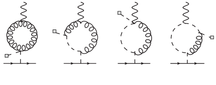
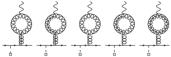
Figure 5: One-particle reducible diagrams with short-distance contributions.

In fact, there is an entire class of one-particle reducible (1PR) diagrams shown in figure 5, which generates only terms $\propto q^{\mu}\gamma_{5}$. The diagrams in the first row give a short-distance contribution if the internal Higgs propagator connecting to the fermion line is cancelled. In this case the contributions are finite and have exactly the same structure as the $q^{\mu}$ term arising from the diagrams of figure 2 discussed above. The diagrams in the second row of figure 5 are different in that they are not only gauge dependent but also suffer from UV divergences. This is not a problem per se as the anapole moment is known to have both features already in the SM [30]. In any case, we do not have to consider the contributions from the self-energy like 1PR diagrams further, since we are not interested in the anapole moment.

3.3.6 Numerical evaluation

The evaluation of the Wilson coefficient of the electromagnetic dipole operator requires the numerical evaluation of up to four-dimensional integrals. The integration variables are typically three 5D coordinates and the modulus of the loop momentum. For $l\gg T$ the Bessel functions in the propagators behave like exponentials and it is possible to determine the asymptotic behaviour of the integrand analytically. The numerical integration of the integrand in the high-momentum region is time-consuming and introduces significant uncertainties. The origin of this problem is large cancellations between the different Bessel functions in the propagators. Thus, we perform the 5D position integrals over the whole (length) of the fifth dimension, but limit the integral over the modulus of the momentum to the region below some momentum cut-off. In the high-momentum region we replace the integrand by its leading asymptotic behaviour, and integrate it from the cut-off to $l=\infty$. In practice a cut-off of $\mathcal{O}(100T)$ is already sufficiently high. In order to estimate the uncertainty associated with this approximation we vary the cut-off in the interval from $60T$ to $150T$; the typical uncertainties are of the order of a few per mille.

Some of the propagator functions feature discontinuous behaviour if two bulk coordinates coincide (see appendix A.3). Both speed and precision of the evaluation can be improved by explicitly splitting the integration domain into sectors where the integrand is continuous. This approach appears to be slightly more efficient than using a coordinate transformation to make the discontinuities manifest by mapping them onto the coordinate axes. Separating the different regions leads to a reduction of uncertainties by about a factor of 2 to 10, depending on the amount of discontinuous propagators (and thus regions) in the diagram.

The calculation is performed in general covariant gauge. Since the gauge invariant subsets of Feynman diagrams are known (see Sec. 3.3.4) a numerical verification of gauge invariance provides a powerful check for our code. Furthermore, the error estimates provided by standard integration routines can be checked by using the small spurious residual dependence of $\Delta a_{\mu}$ on the gauge parameter $\xi$. Very large gauge parameters are numerically difficult to handle, but the limit $\xi\to\infty$, i.e. unitary gauge, can be performed analytically on the level of propagators and gives consistent results. For the error estimates we typically choose $\xi=1$ and $\xi=4$ as reference gauge parameters. This choice already changes the contributions of individual diagrams significantly and provides a reliable check on the gauge-independence of the sum within numerical uncertainties. For instance, the result for the gauge invariant set of diagrams with an internal hypercharge boson (B1-B5b) varies by one to three percent when changing the the gauge parameter by a factor four, while the individual diagrams experience changes of order one. A similar behaviour is found for the genuinely non-abelian diagrams (W4-W10); here the variation of the sum does not exceed two percent. The abelian $W$ diagrams also form a gauge invariant subset. However, the sum of W1, W2 and W3 is over two orders of magnitude smaller than the individual diagrams. This large cancellation makes the result numerically unstable and prohibits a check of the $\xi$ independence. Due to this cancellation the abelian $W$ diagrams are not important for the determination of $\Delta a_{\mu}$.

It should be noted that the gauge invariance proof in Sec. 3.3.4 does not discriminate between “on-shell” and “off-shell” terms as it takes into account the full propagator of the external fermion. That is, only the sum of both sets of terms needs to be gauge invariant. Indeed we find numerically that the “off-shell” terms alone are $\xi$-dependent, but we checked analytically that the gauge-dependent terms are of the form $(p+p^{\prime})^{\mu}$ and hence can combine with the other terms to a gauge-independent result. Due to the relative smallness of the “off-shell” terms (see also Sec. 4.1) it is not possible to verify within the numerical accuracy that the on-shell terms contain a tiny residual gauge-dependence that cancels this $\xi$-dependence. The analytic proof, however, shows that this must be the case.

As a further check we work with two separate implementations of our evaluation strategy, which both rely on Mathematica to handle the numerical integrations. After combining the uncertainty due to the extrapolation and the error estimate for the integration itself, we determine $\Delta a_{\mu}$ with a typical uncertainty at the percent level. The overall evaluation time generally depends on the specific choice of the 5D input parameters and the desired precision; a typical runtime for the results presented in Sec. 4 is $18\,$hours on an Intel i7-950 3.4 GHz processor.

3.4 Genuine Higgs-exchange contributions

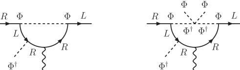
Figure 6: Higgs boson exchange diagrams. The diagram on the left does not exist, since there is no $\Phi\Phi$ propagator. The leading contributions come from higher-dimension operators generated by diagrams such as the right one.

We note that the diagrams in figure 2 contain internal Higgs lines, but they do not correspond to the usual Higgs exchange contributions. For example, the SM Higgs contribution to $(g-2)_{\mu}$ is not part of the zero mode contributions of these diagrams.

The Higgs exchange diagrams with an internal insertion, such as shown in figure 6 left, cannot exist at the level of dimension-six operators $\bar{L}\Phi\sigma_{\mu\nu}EF^{\mu\nu}$, since the internal Higgs propagator would correspond to the (non-existing) $\Phi\Phi$ contraction of the Higgs doublet, while the external line would be $\Phi^{\dagger}$ rather than $\Phi$. The leading Higgs exchange contribution with all Higgs interactions in the loop are generated at one loop by diagrams such as in figure 6 right. This corresponds to dimension-8 operators of the form

$$\frac{1}{T^{4}}\times[y^{\rm(5D)}y^{\rm(5D)\dagger}y^{\rm(5D)}]_{ij}\,\bar{L}_{i}\Phi\sigma_{\mu\nu}E_{j}F^{\mu\nu}\Phi^{\dagger}\Phi\,,$$ (71)

and implies an additional $v^{2}/T^{2}$ suppression relative to the gauge-boson contribution. The loop integral is infrared divergent due to the two (massless) Higgs propagators, which results in an additional logarithm of $T$, similar to the $\ln\,(m_{H}/m_{\mu})$ in the SM Higgs contribution.

In the present paper, we do not address dimension-8 operators. The above operator, generated by Higgs exchange, despite being suppressed, may, however, be of interest for flavour-changing processes, since it depends on the flavour structure $yy^{\dagger}y$ of Yukawa couplings, whereas the dimension-6 operators are proportional to a single Yukawa matrix [16]. However, there are contributions involving $yy^{\dagger}y$ already at the dimension-6 level as we discuss next.

3.4.1 Wrong-chirality Higgs couplings

The diagrams in figure 7 have an external Higgs insertion, which allows for an internal Higgs propagator. However, they contain either chiral components of the brane-to-brane fermion propagator that naively vanish because of $f_{E_{j}}^{(n)}(1/T)=g_{L_{i}}^{(n)}(1/T)=0$, or require the external fermion propagator to be an on-shell zero-mode. We now discuss that in both cases there is a non-vanishing contribution to the matching coefficient of the dimension-six electromagnetic dipole operator, but argue that it is numerically small relative to the gauge-boson exchange term.

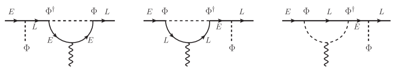
Figure 7: Non-vanishing Higgs-boson exchange diagrams. The diagrams require either a wrong-chirality Higgs coupling or the cancellation of the external propagator.

A sharp delta-function localized Higgs profile leads to ambiguities in the interactions with 5D fields. In the KK-decomposed theory, after electroweak symmetry breaking, this becomes evident, when one solves the mode equations for the fermions [33]. In the 5D unbroken theory the problem arises from the discontinuities of the 5D propagators at coincident points, when these points approach the TeV brane coordinate $z=1/T$. To avoid these ambiguities it is required to define the brane localized minimal RS model by the limit of a model with a regularized Higgs profile with a small width $\delta/T$, where $\delta\ll 1$ as discussed in [20, 21, 18]. Since the fermion modes $f_{E_{j}}^{(n)}(z)$ and $g_{L_{i}}^{(n)}(z)$ vanish only directly on the brane, the finite width of the Higgs profile leads to a non-vanishing coupling of the left-handed singlet and right-handed doublet modes to the Higgs field, which is referred to as wrong-chirality Higgs coupling (WCHC). The treatment of these couplings is subtle, since it involves very high KK excitations with $n\sim 1/\delta$, such that the limits of mode number to infinity and Higgs regulator to zero do not necessarily commute [21]. Since we use 5D propagators, all KK modes are already summed, that is, we implicitly take the limit of the Higgs regulator $\delta$ to zero after the sum over all KK modes. We comment below on how the presence of a cut-off on the scale of validity of the RS model might affect our result.

It is convenient to consider a simple step-function Higgs profile of the form

$$\Phi(x,z)=\Phi(x)\,\frac{T}{\delta}\,\Theta(z-(1-\delta)/T)$$ (72)

with a dimensionless parameter $\delta\ll 1$. This choice for the profile and, up to small corrections of order $v^{2}/T^{2}$, also for the Higgs vacuum expectation value allows for an analytical calculation of the Higgs-exchange diagrams. Note that we consider (72) as a regularization of the minimal RS model, implying $\delta\to 0$ in the end, and hence do not need to address the question which dynamics might generate this profile as a solution to the field equations.

We calculate the diagrams shown in figure 7 starting from an expression, where all three Higgs vertices are delocalized. In the limit $\delta\to 0$, we find that the resulting contribution to the matching coefficient $a_{ij}$ of the electromagnetic dipole operator takes the simple expression

$$\frac{1}{T^{2}}\,a_{ij}^{\rm WCHC}=\frac{c\,e}{16\pi^{2}}\frac{1}{T^{2}}\times\frac{T^{3}}{k^{4}}\,f_{L_{i}}^{(0)}(1/T)[YY^{\dagger}Y]_{ij}g_{E_{j}}^{(0)}(1/T)\,,$$ (73)

where $c=-\frac{1}{12}$ is a constant that can be computed analytically, and $Y_{ij}=y^{(\rm 5D)}_{ij}k$ is the dimensionless 5D Yukawa matrix. The expression after the $\times$ symbol is dimensionless and depends on the 5D mass parameters $c_{E_{j}}$, $c_{L_{i}}$ and scales $k$, $T$ only through the 4D Yukawa matrix $y_{ij}$, since

$$f_{L_{i}}^{(0)}(1/T)g_{E_{j}}^{(0)}(1/T)=\frac{k^{4}}{T^{3}}\,\frac{y_{ij}}{Y_{ij}}\,,$$ (74)

see (13). The presence of three Yukawa matrices makes these diagrams particularly important for lepton-flavour changing observables. The details of the calculation and the flavour aspects will be presented in [34].

The contribution of (73) to $g_{\mu}-2$ is more model-dependent than the gauge-boson contributions as there is no general argument that connects the size of the elements of $Y$ to those of the product $YY^{\dagger}Y$. In the model with all entries of $Y$ of the same order, and assuming no cancellations that introduce structure to the product of three anarchic Yukawa matrices, we can use the current bound on the $\mu\to e\gamma$ decay rate [35], which involves exactly the same diagrams, to constrain the product of Yukawa factors and $T^{-2}$. This leads to a rough upper limit on the size of the Higgs-exchange contribution to $g_{\mu}-2$,

$$\Delta a_{\mu}^{\rm WCHC}\leq 2\cdot 10^{-12}\,,$$ (75)

which is independent of the KK scale $T$. Thus, Higgs exchange is always irrelevant phenomenologically unless there is a significant enhancement of the Yukawa coupling factor relevant to the muon anomalous magnetic moment relative to the anarchic estimate. If we abandon the assumption of anarchy as might be suggested by the strong constraint from lepton flavour violation, we cannot use the $\mu\to e\gamma$ decay rate to constrain the Higgs contribution to $a_{\mu}$ as the two observables are not governed by the same model parameters. However, the requirement that the Higgs contribution does not exceed the present experimental measurement of $\Delta a_{\mu}$ still imposes a constraint on the product of Yukawa couplings as will be discussed in the next section.

Since the RS models should be defined as an effective theory with cut-off $\Lambda\gg T$, it may be argued that the KK sum should be truncated once the KK masses exceed $\Lambda$, and that the loop momentum in the diagrams of figure 7 should be restricted to values smaller than the cut-off. When the brane-localization limit $\delta\to 0$ is taken at fixed $\Lambda$, the wrong-chirality Higgs-coupling contribution to $g_{\mu}-2$ vanishes. Alternatively, we may interpret brane localization as $\delta\sim T/\Lambda\ll 1$, in which case there is no simple analytic result for $a_{ij}^{\rm WCHC}$, but the magnitude is similar to (73). Thus, the rough bound (75) should remain valid independent of the precise relation between $\delta$ and $\Lambda$ and the order of limits. The different treatments of the order of limit amounts to a different definition of the meaning of “brane localization” and hence the model itself. The Higgs-exchange contribution (contrary to the gauge boson exchange contribution discussed later) is therefore model-dependent. A similar situation arises in the calculation of Higgs production [20, 21].

There is another Higgs contribution to electromagnetic dipole transitions at order $1/T^{2}$ that arises from the class-1 operator $h_{ij}\bar{L}_{i}\Phi E_{j}\Phi^{\dagger}\Phi+\mbox{h.c.}$, which was not included in (10), since $h_{ij}$ is non-zero only when the wrong-chirality Higgs couplings are taken into account. Tree-level matching with the step-function Higgs profile (72) gives the coefficient function (see also [23])

$$\frac{1}{T^{2}}\,h_{ij}=\frac{1}{3T^{2}}\times\frac{T^{3}}{k^{4}}\,f_{L_{i}}^{(0)}(1/T)[YY^{\dagger}Y]_{ij}g_{E_{j}}^{(0)}(1/T)\,,$$ (76)

which differs from (73) only by the absence of the electromagnetic coupling and the loop factor. When two of the Higgs fields in $\bar{L}_{i}\Phi E_{j}\Phi^{\dagger}\Phi$ are put to their vacuum expectation values, this operator modifies the Yukawa couplings and leads to flavour-changing couplings of the zero-mode fermions to the Higgs boson. Inserting this vertex into the Higgs-exchange contribution to the electromagentic dipole transition similar to diagrams c and d of figure 1, we find that the result is suppressed relative to (73) by a factor of [lepton mass]${}^{2}/m_{H}^{2}$, where $m_{H}$ is the physical Higgs mass. The additional lepton mass factors arise from the 4D Yukawa coupling at one of the Higgs-fermion vertices and the need for a helicity flip in the loop. Thus, the Higgs-exchange contribution to the anomalous magnetic moment and to radiative lepton flavour violating transtions from loop momentum $k\sim m_{H}$ is strongly suppressed relative to the contribution (73) that is generated at the KK scale.

3.4.2 Off-shell Higgs diagrams

Each of the three diagrams in figure 7 also contains “off-shell” contributions of the type discussed in Sec. 3.3.2, where the external zero-mode propagator is cancelled, resulting in a local short-distance contribution. Since the zero mode always has the right chirality, the “off-shell” terms do not involve wrong-chirality Higgs couplings, and we can work with a brane-localized Higgs field from the start. Then the diagrams involve at most one bulk coordinate integral from the photon vertex. This integral can be taken analytically, as well as the remaining integral over the loop momentum. Here it proves useful to use the KK decomposition of the internal fermion propagators. The zero mode has to be subtracted from the internal propagators, since their contribution cannot be associated with the KK scale $T$. This subtraction also renders the loop integral infrared finite.

The dependence on lepton flavour of the off-shell terms is of the form

$$\sum_{k}f_{L_{i}}^{(0)}(1/T)Y_{ih}[Y^{\dagger}]_{hk}Y_{kj}[f^{(0)}_{L_{k}}(1/T)]^{2}g_{E_{j}}^{(0)}(1/T).\vspace*{-0.4cm}$$ (77)

Due to the extra factor $[f^{(0)}_{L_{k}}(1/T)]^{2}$ there is now a strong dependence on the bulk mass parameters in addition to the explicit form of the Yukawa matrices, which makes it difficult to give a precise estimate for the off-shell Higgs contribution to $(g-2)_{\mu}$. For the symmetric choice of bulk mass parameters, $c_{E_{k}}=-c_{L_{k}}$, we expect the product $[f^{(0)}_{L_{k}}(1/T)]^{2}$ to count as a factor of lepton mass $m_{\ell_{k}}$; in this case the “off-shell” contribution is small relative to the WCHC contribution. In general, it can be of similar size. In principle this would allow for a flavour-specific cancellation between the two contributions, that is, a cancellation for $\mu\to e\gamma$, but not for the flavour-diagonal quantity $(g-2)_{\mu}$, in which case the bound (75) is invalidated. However, if we assume that the bulk mass parameters and anarchic Yukawa matrices do not conspire in this way, the sum of all three “off-shell” Higgs diagrams is two orders of magnitude smaller than the experimental uncertainty on $a_{\mu}$, and hence negligible.

3.5 Wrong-chirality Higgs couplings in gauge boson diagrams

Naturally the question arises whether there exist contributions with WCHCs in the gauge boson exchange diagrams of figure 2. Inspection shows that only the internal insertion diagrams B1a/b and B3a/b contain non-vanishing wrong-chirality Higgs-fermion vertices, once the Higgs profile is regulated by a finite width. The following analysis demonstrates, however, that these contribution vanish as ${\cal O}(\delta)$, when the Higgs profile regulator $\delta$ is removed. This should be contrasted to the case of the Higgs-exchange diagrams discussed above, where the finite contribution (73) survives in the $\delta\to 0$ limit.

We analyze the loop momentum integrand in the two regions $l\ll T/\delta$ and $l\gg T/\delta$ according to whether the loop momentum is much smaller (larger) than the width of the Higgs profile at the TeV brane. We assume $\delta\ll 1$ and hence $T/\delta\gg T$. For concreteness, we consider only a single term in the complete expression for diagram B1a; the following arguments are general and also apply to the other terms and diagrams. Consider therefore the expression

$$\int\frac{d^{4}l}{(2\pi)^{4}}\;\int_{1/k}^{1/T}\!\!\!\frac{dy}{(ky)^{4}}\int_{1/k}^{1/T}\!\!\!\frac{dw}{(kw)^{4}}\int_{1/k}^{1/T}\!\!\!\frac{dx}{(kx)^{4}}\int_{(1-\delta)/T}^{1/T}\!\!\!dz\,\frac{T}{\delta}\,$$

$$\times\Delta^{\rm ZMS}_{\perp}(l,x,w)\,F_{L}^{-}(l,x,y)\;d^{+}F_{L}^{-}(l,y,z)\;d^{+}F_{E}^{-}(l,z,w)\,.$$ (78)

The wrong-chirality Higgs coupling appears at the vertex with bulk coordinate $z$, which is confined to $z\in(\frac{1-\delta}{T},\frac{1}{T})$ due to (72). Each of the propagators $d^{+}F_{L}^{-}(l,y,z)$ and $d^{+}F_{E}^{-}(l,z,w)$ vanishes if $z$ is exactly equal to $1/T$.

Let us start with the region of loop momentum much smaller than the inverse Higgs profile width $T/\delta$, in which case we can expand the wrong-chirality propagator functions for $l(1/T-z)\ll 1$ and $l/k\ll 1$. An important point is that propagator functions such as (see (148c))

$$d^{+}F^{-}_{L}(l,y,z) = -l\,\Theta(y-z)\,\frac{ik^{4}y^{5/2}z^{5/2}\tilde{S}_{+}(l,y,1/T,c_{L})S_{-}(l,z,1/k,c_{L})}{S_{-}(l,1/T,1/k,c_{L})}$$ (79)

$$-\,l\,\Theta(z-y)\,\frac{ik^{4}y^{5/2}z^{5/2}S_{-}(l,z,1/T,c_{L})\tilde{S}_{+}(l,y,1/k,c_{L})}{S_{-}(l,1/T,1/k,c_{L})}$$

are discontinuous at $y=z$. The second term is ${\cal O}(\delta)$, since $S_{-}(l,1/T,1/T,c_{L})=0$ and $z$ is within distance $\delta/T$ near $1/T$, while the first one is ${\cal O}(1)$. But the first term is only operative, when $y>z$, which constrains $y$ to be within the narrow Higgs profile. This immediately leads to the following counting for the four different orderings for the coordinates $z$,$w$ and $y$ (the arguments of the critical propagator functions): (a) $z>y,w$, (b) $y>z>w$, (c) $w>z>y$ and (d) $y,w>z$.

• For $z>y,w$ the product $d^{+}F_{L}^{-}(l,y,z)d^{+}F_{E}^{-}(l,z,w)$ is of order $\delta^{2}$. The $z$-integral provides a power of $\delta$ from the length of the integration interval and $T/\delta$ from the height of the Higgs profile, so the whole contribution from (a) vanishes as $\delta^{2}$ for $\delta\to 0$.

• In case of $y>z>w$, $d^{+}F_{E}^{-}(l,z,w)$ still counts as ${\cal O}(\delta)$, but $d^{+}F_{L}^{-}(l,y,z)$ loses its suppression factor, since now the first line of (79) is the relevant one. Hence, $d^{+}F_{L}^{-}(l,y,z)d^{+}F_{E}^{-}(l,z,w)\sim\delta$. Now note that the requirement $y>z>w$ means that $y$ must be in $(\frac{1-\delta}{T},\frac{1}{T})$, so the $y$ integration interval counts as $\mathcal{O}(\delta)$. Collecting all factors of $\delta$, we see that the loop momentum integrand again scales as $\delta^{2}$.

• For $w>z>y$ the counting is obviously analogous to (b).

• For $y,w>z$ both propagators lose their $\delta$ suppression. However, both, the $y$ and the $w$ integration, are now limited to the interval $(\frac{1-\delta}{T},\frac{1}{T})$. This restores the overall factor of $\delta^{2}$.

We see that irrespective of the ordering of bulk coordinates, the loop momentum integrand vanishes as $\delta^{2}$ for $\delta\to 0$ in the momentum region $l\ll T/\delta$. As this point we expand the propagator functions in $l\gg T$ and $l/k\ll 1$ and find that after carrying out the angular integration the loop momentum integrand is nearly constant (that is, ${\cal O}(l^{0})$) over the interval from $l\sim T$ to $l\sim T/\delta$. Hence the final integral over $dl$ provides a factor $1/\delta$ and the entire diagram with loop momentum cut off at $T/\delta$ vanishes as ${\cal O}(\delta)$ when the Higgs profile regularization is removed.

It remains to estimate the contribution from very large loop momentum. When $l\gg T/\delta$ (but still $l\ll k$) we find that the propagators exhibit universal behaviour. Let $\Delta$ be the distance between starting and end point of the propagation in the fifth dimension. Then the propagators all behave as $e^{-l\Delta}$. Hence, the coordinate integrals have support only if all coordinates are within a typical distance of order $1/l$ of each other; otherwise the integrand is exponentially small. Changing the integration variables from $(x,y,z,w)$ to $(z,z-w,w-x,x-y)$ we see that each integration over distance differences, e.g. $z-w$, counts as $1/l$. Only the $z$ integral gives a factor of $\delta/T$ that is cancelled by the Higgs profile height $T/\delta$. Collecting all factors shows that after integration over the bulk coordinates the remaining loop-momentum integrand is independent of $\delta$ and scales as $dl/l^{2}$. Thus the integration over $l$ from $T/\delta$ to infinity scales as $\delta$. This proves that the entire expression (3.5) vanishes in the limit $\delta\to 0$, when the regularization of the Higgs brane localization is removed.

In a similar fashion all other terms with wrong-chirality Higgs couplings in gauge boson exchange diagrams can be shown to vanish in the limit $\delta\to 0$, so no correction needs to be applied to the calculation performed in the model with an exactly brane-localized Higgs field.

4 Muon anomalous magnetic moment

4.1 Single-flavour approximation for gauge boson diagrams

We now discuss our result for the muon anomalous magnetic moment. We will mostly restrict ourselves to the single-flavour approximation, and discuss briefly below why it should be a good approximation to neglect lepton-flavour changing contributions for the gauge boson diagrams.

In this case the matching coefficients $\alpha\equiv\alpha_{22}$ (dipole operator) and $\beta\equiv\beta_{2222}$ (four-fermion operator) defined in (16) are functions of $k$, $T$, the two bulk-mass parameters $c_{L}$, $c_{E}$, and the dimensionless 5D Yukawa coupling $Y_{\mu}\equiv y^{\rm(5D)}_{22}k$. We fix the Planck scale quantity $k$ to $2.44\times 10^{18}\,$GeV [7], and determine $c_{E}$ from the value of the muon mass $m_{\mu}=105.7\,$MeV through (13), for given $T$, $c_{L}$, and $Y_{\mu}$. The other parameters that enter the analysis are the Weinberg angle $s_{W}^{2}=\sin^{2}\theta_{W}=0.231$, the electromagnetic coupling $\alpha_{\rm em}(M_{Z})=1/128.94$, and the Higgs vacuum expectation value $v=246\,$GeV.

The contribution to the anomalous magnetic moment from the four-fermion operator follows from (27) and (34):

$$[\Delta a_{\mu}]_{\rm 4f}=-\frac{m_{\mu}^{2}}{T^{2}}\,\frac{\beta}{4\pi^{2}}=\frac{\alpha_{\rm em}}{8\pi c_{W}^{2}}\,\frac{m_{\mu}^{2}}{T^{2}}\,\frac{1}{\ln\frac{1}{\epsilon}}\,f(\epsilon,c_{L},c_{E})\approx 1.2\cdot 10^{-13}\,\times(1\,\mbox{TeV}/T)^{2}.$$ (80)

In the last expression we adopted $T=1\,$TeV and symmetric bulk mass parameters $c_{L}=-c_{E}=0.578\ldots$, which leads to $f=0.95$, and made the dominant dependence on $T$ explicit. Thus, the four-fermion operator makes a negligible contribution to the anomalous magnetic moment compared to the dipole operator discussed below, mainly due to the $1/\ln(1/\epsilon)\approx 1/35$ suppression. We find that $f\approx 1$ is always a good approximation, independent of the values of $T$ and $Y_{\mu}$, when the bulk mass parameters are near the symmetric value. This can be different when $c_{L}$ is larger than about 0.65, or smaller than 0.5, but (except for extreme choices of $c_{L}$ where $c_{E}$ becomes positive) $f$ is never large enough to compensate the $1/\ln(1/\epsilon)$ suppression. Therefore we drop the four-fermion operator contribution from the further discussion.

The contribution from the electromagnetic dipole operator is determined by five-dimensional loop integrals. For their evaluation we have to rely on numerical integration and must add (60) to take the additional term from W8 into account. Before discussing the result, we provide an order-of-magnitude estimate of this contribution. Since the loop is dominated by momenta of order of the KK scale $T$, one might expect the dimensionless Wilson coefficient $\alpha_{22}$ in (16) to be of order $e\times\alpha_{\rm em}/(4\pi)$. According to (27) this would result in $\Delta a_{\mu}\sim\alpha_{\rm em}/(4\pi)\times(m_{\mu}v)/T^{2}\approx 1.6\cdot 10^{-8}\times(1\,\mbox{TeV}/T)^{2}$, which is very large. This estimate is, however, too naive as it does not take into account the wave functions of the external 5D states. The photon zero-mode profile (113) provides a factor of $1/\sqrt{\ln(k/T)}$. The conversion factors for the gauge couplings $g_{5}^{(\prime)}\to g_{4}^{(\prime)}$ amount to $\ln^{3/2}(k/T)$, since the one-loop diagrams involve three gauge couplings. Thus, we obtain an overall factor $\ln\left(1/\epsilon\right)$. Furthermore, the external fermion zero-modes provide a factor of $g_{E}^{(0)}(x)f_{L}^{(0)}(z)$. Since the integrals over the bulk coordinates are dominated by $x,z\sim 1/T$, we expect that $\alpha_{22}$ is roughly proportional to $g_{E}^{(0)}(1/T)f_{L}^{(0)}(1/T)$. Together with the vacuum expectation value $v/\sqrt{2}$ in (27) from the Higgs insertion, this counts as a factor of order $m_{\mu}$. The contribution to $\Delta a_{\mu}$ due to electromagnetic dipole operators is then estimated by

$$\Delta a_{\mu}\approx\frac{\alpha_{\rm em}}{4\pi}\,\frac{m_{\mu}^{2}}{T^{2}}\,\ln\left(1/\epsilon\right)\times{\rm Loop}(c_{L},c_{E},y^{\rm(5D)},T,\epsilon)\,,$$ (81)

where the remaining loop factor should be $\mathcal{O}(1)$. This estimate indicates that the contribution from the dipole operators is enhanced by a factor of the order $\ln^{2}\left(1/\epsilon\right)\sim 10^{3}$ compared to the contribution from the four-fermion operator; this would lead to $\Delta a_{\mu}\approx 2.4\cdot 10^{-10}$ for $T=1\,\rm TeV$, which is only a factor of three smaller than the present uncertainty of $a_{\mu}$.

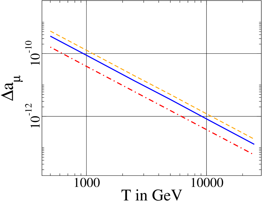
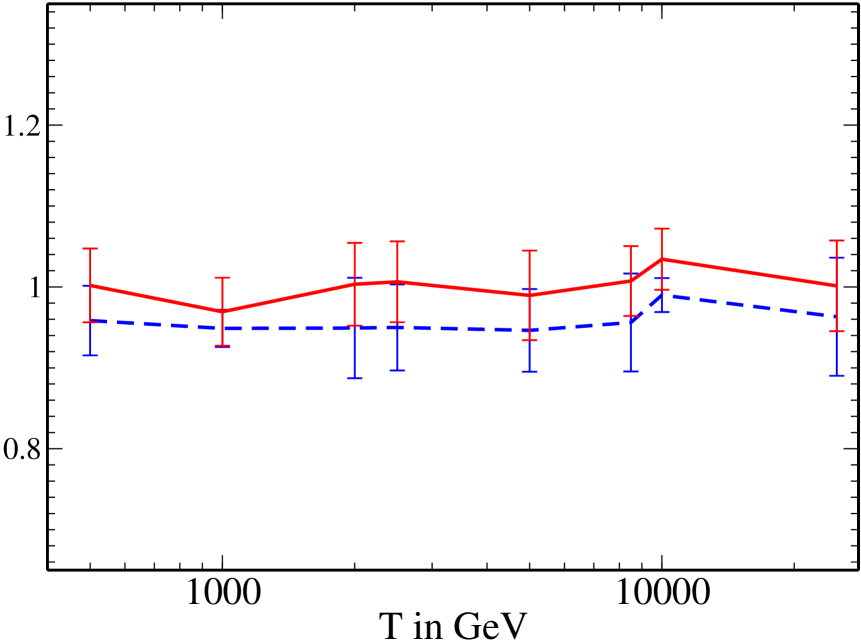
Figure 8: Left panel: Dependence of the different contributions to $\Delta a_{\mu}$ on the KK scale $T$: $-[\Delta a_{\mu}]_{B}$ (dark grey/red, dot-dashed), $[\Delta a_{\mu}]_{W}$ (light-grey/orange, dashed) and the sum (black/blue, solid). Right panel: $\Delta a_{\mu}(c_{L},Y_{\mu})/\Delta a_{\mu}(c_{L}=-c_{R}=0.578425,Y_{\mu}=1)$ for $c_{L}=0.51,Y_{\mu}=1$ (dashed) and $c_{L}=-c_{R},Y_{\mu}=10$ (solid) as a function of $T$.

For our numerical study it is convenient to split $\Delta a_{\mu}$ in contributions from an exchange of hypercharge $B$ bosons and $W$ bosons

$$\Delta a_{\mu}=[\Delta a_{\mu}]_{B}+[\Delta a_{\mu}]_{W}\;$$ (82)

and to study them separately. The left panel in figure 8 shows the $T$ dependence of $-\left[\Delta a_{\mu}\right]_{B}$ (dot-dashed) and $\left[\Delta a_{\mu}\right]_{W}$ (dashed) as well as the sum (solid) for the parameter choice $c_{L}=-c_{E}$ and $Y_{\mu}=1$. Note that the contribution due to hypercharge bosons $B$ has opposite sign than the non-abelian contribution. The dependence of $\Delta a_{\mu}$ on $T$ follows almost precisely the $1/T^{2}\times\ln(k/T)$ scaling, see (81). Fitting the numerical $T$ dependence shown in figure 8 to $1/T^{\,x}\times\ln(k/T)$ one finds a best fit for $x=1.997\pm 0.04$. The contribution of (60) to $\left[\Delta a_{\mu}\right]_{W}$ is typically at the level of $2.5\%$. This is consistent with the absence of a $\ln(k/T)$ enhancement in (39). The left panel shows the result for $\Delta a_{\mu}$ for different choices of $c_{L}$ and $Y_{\mu}$ normalized to $\Delta a_{\mu}(c_{L}=-c_{E},Y_{\mu}=1)$. We see that the ratio is quite independent of the KK scale: the $T$ dependence is practically universal. Also different choices of $c_{L}$ and $Y_{\mu}$ change $\Delta a_{\mu}$ only mildly.

From figure 8 we conclude not only that the correction to $g_{\mu}-2$ is quite insensitive to the specific choice for $y^{(5D)}$ and the mass parameters $c_{L}$ and $c_{E}$, but also that the estimate (81) agrees fairly well with the numerical results if not for some amount of cancellation between $[\Delta a_{\mu}]_{W}$ and $[\Delta a_{\mu}]_{B}$. Explicit numerical values for a representative set of parameters are shown in table 1 where a reference value of $T=1\,\rm TeV$ was used.

	$Y_{\mu}$	$c_{L}$	$c_{E}$	$\left[\Delta a_{\mu}\right]_{B}$	$\left[\Delta a_{\mu}\right]_{W}$
	$0.1$	$0.53605$	$-0.53605$	$-4.18(08)\cdot 10^{-11}$	$1.27(2)\cdot 10^{-10}$
	$0.25$	$0.553805$	$-0.553805$	$-4.31(19)\cdot 10^{-11}$	$1.29(1)\cdot 10^{-10}$
	$1$	$0.578425$	$-0.578425$	$-4.02(10)\cdot 10^{-11}$	$1.28(1)\cdot 10^{-10}$
	$4$	$0.601598$	$-0.601598$	$-4.05(15)\cdot 10^{-11}$	$1.29(1)\cdot 10^{-10}$
	$10$	$0.616446$	$-0.616446$	$-4.34(08)\cdot 10^{-11}$	$1.29(2)\cdot 10^{-10}$
	$1$	$0.51$	$-0.634898$	$-4.13(10)\cdot 10^{-11}$	$1.28(2)\cdot 10^{-10}$
	$1$	$0.55$	$-0.604918$	$-4.20(15)\cdot 10^{-11}$	$1.27(3)\cdot 10^{-10}$
	$1$	$0.578425$	$-0.578425$	$-4.02(10)\cdot 10^{-11}$	$1.28(1)\cdot 10^{-10}$
	$1$	$0.6$	$-0.555607$	$-4.26(16)\cdot 10^{-11}$	$1.29(2)\cdot 10^{-10}$
	$1$	$0.64$	$-0.501419$	$-4.06(10)\cdot 10^{-11}$	$1.28(3)\cdot 10^{-10}$

Table 1: Dependence of the contributions to $\Delta a_{\mu}$ on mass parameter asymmetry and Yukawa coupling. $T$ has been fixed to $1\,\rm TeV$. The uncertainties include the numerical error from the integration, and the uncertainty from the extrapolation and residual $\xi$ dependence.

The robustness of the result with respect to the 5D parameters can be understood in the following way. Consider the contribution from terms that do not have a fermion zero-mode propagator. As already mentioned above each external (SM) fermion comes with the corresponding zero-mode profile; in our case $g_{E}^{(0)}$ and $f_{L}^{(0)}$ and we expect these mode factors together with the Yukawa to combine roughly into a factor of the lepton mass. The dependence on the 5D parameters will then arise from the zero-mode subtracted fermion propagators. Since the KK modes are quite insensitive to the 5D mass parameters the dependence is, as observed, mild.

Contributions from terms containing an explicit fermion zero-mode propagator, such as the so-called “off-shell” contributions or the IR sensitive part of W8 have two additional zero-mode factors; for instance

$$Y_{\mu}\,g_{E}^{(0)}(1/T)f_{L}^{(0)}(1/T)\cdot f_{L}^{(0)}(x)f_{L}^{(0)}(z)\sim\frac{m_{\ell}}{v}\cdot f_{L}^{(0)}(x)f_{L}^{(0)}(z).$$ (83)

The product $f_{L}^{(0)}(x)f_{L}^{(0)}(z)$ is very sensitive to the choice of the 5D mass parameters and one expects a much more pronounced dependence on 5D masses and Yukawa couplings. However, as already argued in Sec. 3.3.2 these terms will typically be suppressed and, hence, this effect is not seen in the total.

We will illustrate this using the non-abelian diagrams as an example. Consider the two special cases: a fixed doublet 5D mass such that $c_{L}=0.5$ and the symmetric choice $c_{L}=-c_{E}$. In all non-abelian diagrams contributing to the $\bar{L}\sigma_{\mu\nu}EW^{\mu\nu}$ structure the actual loop is independent of $c_{E}$; thus after fixing $c_{L}=0.5$ the remaining dependence on $c_{E}$ from the external lines and on $Y_{\ell}$ will always combine to a factor of the lepton mass $m_{\ell}$ – irrespective whether a zero-mode propagator is involved or not. For the symmetric choice $c_{L}=-c_{E}$ the identity $f_{L}^{(0)}(x)=g_{E}^{(0)}(x)$ suggests that the explicit factor $f_{L}^{(0)}(x)f_{L}^{(0)}(z)$ for zero-mode propagators should count as an additional power of $m_{\ell}$ if the loop is dominated by the region very close to the IR brane. In this case the term with a zero-mode propagator will scale like $m_{\ell}^{2}$ rather than $m_{\ell}$ as for the remaining contributions. In particular, the “off-shell” diagrams which by definition have an explicit zero-mode propagator are sensitive to the 5D mass parameters and not necessarily proportional to the lepton mass.

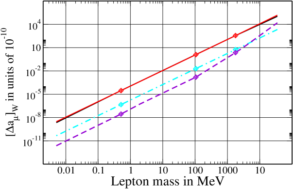
Figure 9: Lepton mass dependence of total non-abelian (solid) and non-abelian “off-shell” contributions to $a_{\mu}$; the dashed line refers to fixed $c_{L}=0.5001$, the dot-dashed one to the symmetric choice $c_{L}=-c_{R}$. Diamonds correspond to electron, muon and tau mass, respectively.

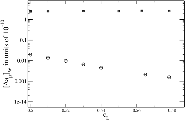
Figure 10: Dependence of $[a_{\mu}]_{W}$ on $c_{L}$. Squares correspond to the sum over all diagrams, circles to the “off-shell” terms only.

To verify whether this intuitive picture is justified we study the lepton mass dependence of $[\Delta a_{\mu}]_{W}$ numerically. Figure 9 shows the full contribution of all $W$ diagrams compared to the contribution of “off-shell” terms as a function of the lepton mass. Both $T=1\;\rm TeV$ and $Y_{\ell}=1$ are kept fixed. The total non-abelian contributions (solid lines) for both, the asymmetric and symmetric case are on top of each other and cannot be distinguished on the logarithmic scale; both are proportional to $m_{\ell}^{2}$. The “off-shell” terms show exactly the same scaling for fixed doublet modes with $c_{L}=1/2$ (dot-dashed line) and are a factor $60$ smaller than the total contribution in agreement with our previous estimate. For $c_{L}=-c_{E}$ (dashed) the lepton-mass dependence is more involved. Following our argument above we expect $m_{\ell}^{3}$ behaviour. This is, however, only realized for lepton masses above $2\,\rm GeV$. For leptons lighter than the muon we find same $m_{\ell}^{2}$ dependence as in the $c_{L}=1/2$ case. The source of this unexpected behaviour can be traced to two diagrams: W1 and W4. Both W1 and W4 contain a contribution where only fermion zero-modes propagate in the loop. Our argument for the expected suppression of the off-shell terms by one additional power of the lepton mass relies on IR-brane dominance of the coordinate integrals due to the localization of the KK modes (see Sec. 3.3.2). For the pure fermion zero-mode contribution this dominance is not present and these terms are only suppressed by a mass-independent factor instead of $m_{\ell}/v$. The zero-mode terms are thus less suppressed for very light leptons and give rise to the $m^{2}_{\ell}$ behaviour in the low mass region of figure 9. The $c_{L}$ dependence of the different contributions to $[a_{\mu}]_{W}$ is illustrated in figure 10. Again sum over all diagrams shows almost no sensitivity whereas the small off-shell terms are quite sensitive to the specific choice for $c_{L}$.

Using the overall dependence on $T^{2}$ and the relative insensitivity to mass parameters and Yukawa couplings we can condense our result for the correction to $(g-2)_{\mu}$ in the minimal RS model into

$$\Delta a_{\mu}\approx 8.8\cdot 10^{-11}\,\times(1\,\mbox{TeV}/T)^{2}\,,$$ (84)

which is our main result. The exact results differ from this approximation by less than 10% for $Y_{\mu}\in(0.1,10)$, $T\in(0.5\,{\rm TeV},50\,{\rm TeV})$ and $c_{L}$ between $0.5$ and the symmetric choice. The difference between the current experimental average of the anomalous magnetic moments of $\mu^{+}$ and $\mu^{-}$ and the Standard Model prediction is given by [36]

$$a_{\mu}^{\rm exp}-a^{\rm SM}_{\mu}=287(63)(49)\times 10^{-11}$$ (85)

where the two errors correspond to the combined experimental and theoretical uncertainties, respectively. Since we find $\Delta a_{\mu}$ to be positive in the RS model, $a_{\mu}^{\rm exp}-a^{\rm RS}_{\mu}$ will be smaller than $a_{\mu}^{\rm exp}-a^{\rm SM}_{\mu}$, decreasing the discrepancy between theory and experiment. However, the estimate (84) shows that for $T>1\;{\rm TeV}$ the correction to $a^{\rm SM}_{\mu}$ is too small. Even for a low KK scale of $T\approx 500\;{\rm GeV}$ which corresponds to lowest KK excitations presently being excluded by direct searches, $\Delta a_{\mu}$ only reaches the level of $40\times 10^{-11}$ — of order of the error on $a_{\mu}$, but too small to reconcile theory and experiment at the $2\sigma$ level.

The above discussion applies to the gauge boson contribution to $a_{\mu}$. In Sec. 3.4 we already showed that in models with anarchic Yukawa matrices the Higgs-exchange contribution is limited to a few times $10^{-12}$, barring accidental cancellations that invalidate the $\mu\to e\gamma$ constraint. Abandoning the anarchy assumption, we may turn the argument around and try to glean some information on the specific product of three Yukawa matrices that enters the Higgs contribution from $g_{\mu}-2$. To this end, we define the dimensionless quantity

$$\langle YY^{\dagger}\rangle_{\mu}=\frac{\operatorname{Re}\left[\sum_{lm}[U^{\dagger}]_{2l}f_{L_{l}}^{(0)}(1/T)[YY^{\dagger}Y]_{lm}g_{E_{m}}^{(0)}(1/T)V_{m2}\right]}{\sum_{lm}[U^{\dagger}]_{2l}f_{L_{l}}^{(0)}(1/T)Y_{lm}g_{E_{m}}^{(0)}(1/T)V_{m2}}\,,$$ (86)

which parametrises the flavour dependence of the contribution from (73) to $g_{\mu}-2$ compared to a term with only a single Yukawa matrix. Note that the denominator of (86) is simply the 4D muon Yukawa coupling $y_{\mu}$. From (27) and (73) we obtain

$$\Delta a_{\,u}^{\rm WCHC}=\frac{1}{48\pi^{2}}\,\frac{m_{\mu}^{2}}{T^{2}}\,\langle YY^{\dagger}\rangle_{\mu}\,.$$ (87)

Adding the gauge-boson contribution this can be written as

$$\Delta a_{\mu}=\left[8.8+2.4\,\langle YY^{\dagger}\rangle_{\mu}\right]\cdot 10^{-11}\,\times(1\,\mbox{TeV}/T)^{2}$$ (88)

With experimental and theoretical errors added linearly, the measurement (85) can then translated into the bound

$$-25<\langle YY^{\dagger}\rangle_{\mu}\times(1\,\mbox{TeV}/T)^{2}<260\,,$$ (89)

where we required that $a_{\mu}^{\rm exp}-a_{\mu}^{\rm RS}$ stays compatible with zero at the $3\sigma$ level. The pronounced asymmetry of upper and lower bound arises from the non-zero value of (85). The limit is rather loose, reflecting the small coefficient of the Higgs contribution, constraining the Yukawa entries to “average values” of around $5$ to $15$ for $T=1\,$TeV. For $\langle YY^{\dagger}\rangle_{\mu}\approx 20$ the Higgs contribution is of the same order as the present theoretical uncertainty on $g_{\mu}-2$, again for $T=1\,$TeV. The bound weakens for larger KK scales.

4.2 Beyond single-flavour

The generalization to the case with three lepton flavours is in principle straightforward: the Yukawa factors have to be promoted to the $3\times 3$ Yukawa matrix and the external muon states have to be represented in the mass basis, see (14). In practice, this complicates the calculation, since it now depends on six bulk mass parameters and the full 5D Yukawa matrix, and only three of these parameters can be eliminated by the known lepton masses. We now argue that this complication is not relevant for the gauge-boson contribution to the anomalous magnetic moment.

In the interaction basis the only source of flavour change is the Yukawa matrix itself. Thus, independent of its topology each Feynman diagram can schematically be written as

$$\sum_{i,j}U^{\dagger}_{ni}M^{(1)}_{ii}y_{ij}^{\rm(5D)}M^{(2)}_{jj}V_{jm},$$ (90)

where $n=m=2$ for external muon states. Here $M^{(1)}$ and $M^{(2)}$ collect all factors depending on only flavour indices $i$ and $j$, respectively. For the single-flavour approximation we observed that the dominant contribution to the dipole-operator Wilson coefficient $\alpha_{ij}$ (and thus to $g_{\mu}-2$) is largely insensitive to the specific choice for the 5D masses or Yukawa couplings but depends linearly on the lepton mass. For the three-flavour case this means that the dominant contribution to $g_{\mu}-2$ is roughly proportional to the mass matrix:

$$\left[M^{(1)}_{ii}y_{ij}^{5D}M^{(2)}_{jj}\right]_{\rm dom}\propto f^{(0)}_{L_{i}}(1/T)y_{ij}^{5D}g^{(0)}_{E_{j}}(1/T)\,.$$ (91)

As the matrices $U$ and $V$ diagonalize the mass matrix

$$\frac{T^{3}}{k^{3}}\frac{v}{\sqrt{2}}\sum_{i,j}\,U^{\dagger}_{ni}f^{(0)}_{L_{i}}(1/T)y_{ij}^{\rm(5D)}g^{(0)}_{E_{j}}(1/T)V_{im}={\rm diag}\left\{m_{e},m_{\mu},m_{\tau}\right\}_{nm}\,,$$ (92)

the flavour dependence of the diagrams approximately combines into a lepton mass factor, irrespective of the specific choices of the bulk mass parameters $c_{L_{i}}$, $c_{E_{j}}$ and 5D Yukawa matrix. Hence we can adopt the simplest choice for the calculation by taking the Yukawa matrix diagonal, which corresponds to the single-flavour approximation. The anomalous magnetic moment of the muon is therefore reliably determined in this approximation, up to small corrections to (91), which are no larger than, e.g., the effect of unaccounted higher dimensional operators.

The fact that (90) is, up to small corrections, already diagonal, implies that lepton flavour-violating transitions are suppressed. Flavour-changing processes – such as $\mu\to e\gamma$ in the lepton sector or $b\to s\gamma$ in the quark sector – are therefore sensitive to the sub-dominant contributions that depend strongly on the 5D mass parameters. Such terms arise, for example, when the internal fermion lines of a diagram propagate zero modes and the gauge boson is a KK mode (see [16]), or via the contribution of the “off-shell” part of the $\bar{L}_{i}L_{i}\gamma$ vertex with a subsequent mass insertion as discussed in the previous section. In this situation the suppression of “off-shell” diagrams is lifted and the terms have to be taken into account. Also Higgs exchange, though related to higher-dimensional operators, is relevant to flavour violation, since its different Yukawa matrix dependence produces terms that are not aligned with the mass matrix [15, 16].

4.3 Comparison to previous work

The first calculation of the muon anomalous magnetic moment in the RS model was done very soon [12] after the invention of the model. The authors used the 4D formalism and computed multiple KK sums. They (incorrectly) concluded that external mass insertion diagrams are suppressed by a factor $(m_{\mu}/M_{\rm KK})^{2}$, which eliminates all diagrams except B1a and B1b in figure 2. In these diagrams a misplaced chiral projector at the photon vertex eliminates one of the two terms in the integrand (167), (168). The final result for the gauge-boson contribution to $\Delta a_{\mu}$ in [12] is opposite in sign to ours, which is consistent with the fact that the abelian hypercharge contribution $[\Delta a_{\mu}]_{B}$ is negative. The final result (84) is, however, dominated by $W$-exchange, which was neglected in [12]. Ref. [12] also considered the Higgs contribution and found that it puts important constraints on the bulk mass parameters. However, their Higgs contribution does not seem to contain the $(v/T)^{2}$ suppression relative to the gauge-boson contribution that is expected on general grounds, see Sec. 3.4, when the wrong-chirality Higgs couplings and “off-shell” terms are neglected as was done [12].

The only other estimate of $\Delta a_{\mu}$ in the RS model with SM model fields in the bulk we are aware of is contained in [37]. The calculation is restricted to a one-loop vertex diagram with KK photon exchange but only zero-mode fermions in the loop. This subset of contributions significantly underestimates the true result, since it is suppressed relative to (81) by a factor $\ln^{2}(1/\epsilon)\sim 10^{3}$ due to a cancellation in the photon KK sum.

The calculations of lepton-flavour violating $\ell_{i}\to\ell_{j}\gamma$ processes [15, 16] involve the same diagram topologies as $(g-2)_{\mu}$, but the restriction to flavour violation allows to make some simplifying assumptions. Ref. [15] works in the KK picture and includes only the first KK excitation, while [16] adopts the 5D formalism as we have done in this paper. These works do not consider external insertion diagrams, though this has been corrected in [29]. The Higgs exchange diagrams that can be neglected for $(g-2)_{\mu}$ provide the dominant source of flavour violation and are found to be of order $1/T^{4}$ (again, in the absence of wrong-chirality Higgs couplings and “off-shell” terms) consistent with (71). Ref. [16] also considers the gauge-boson contributions, but assumes that only internal zero-mode fermions are relevant to flavour violation. Since we have seen that the KK fermions in the loop are by far the dominant contribution to flavour-conserving quantities like $(g-2)_{\mu}$, it would be interesting (but numerically challenging) to investigate how the small non-alignment of these terms feeds into flavour violation.

5 Conclusion

In this paper we performed the first complete calculation of the gauge boson exchange contribution to the muon anomalous magnetic moment in the minimal Randall-Sundrum model. We find that the additional contribution to $a_{\mu}$ is enhanced by a factor $\ln(k/T)$ relative to the naive estimate $\alpha_{\rm em}/(4\pi)\times(m_{\mu}/T)^{2}$, resulting in

$$\Delta a_{\mu}\approx 8.8\cdot 10^{-11}\,\times(1\,\mbox{TeV}/T)^{2}\,,$$ (93)

nearly independent of the bulk mass and Yukawa coupling parameters of the model. For $T\approx 500\,$GeV, which corresponds to first KK excitations around $1.3\,$TeV, this is of order of the theoretical uncertainty on $a_{\mu}$. The minimal RS model is, however, already excluded by electroweak precision tests unless $T$ is much larger, which makes the correction to $g_{\mu}-2$ unobservable. $T$ may be lower in models with custodial symmetry, but in this case the contribution from the extra states remains to be computed. The number given above refers to the model-independent contribution from gauge-boson exchange. We also determined the Higgs-exchange mediated contributions to $(g-2)_{\mu}$; they depend on an unconstrained combination of 5D Yukawa couplings. In anarchic scenarios this combination is constrained by $\mu\to e\gamma$, such that the Higgs contributions to $\Delta a_{\mu}$ are below $2\cdot 10^{-12}$. In the general scenario the Higgs contribution depends strongly on the model parameters. We used this to derive a rough limit on the product of Yukawa factors and KK scale $T$.

The 5D framework developed here can be extended to an investigation of lepton and quark flavour-violating radiative processes in warped geometries that goes beyond the approximations adopted in [15, 16, 17]. We hope to report on such results in the future. On the more formal side, it would be interesting to investigate the proper gauge-invariant regularization and renormalization of the RS model as an effective field theory, and the 5D formalism seems to be the suitable framework.

Acknowledgement

We thank A. Mück for many helpful discussions. We also thank K. Agashe, C. Delaunay, and R. Sundrum for their comments on wrong-chirality Higgs couplings. MB and JR thank the Kavli Institute for Theoretical Physics at UC Santa Barbara for hospitality, while part of this work was done. This work is supported in part by the Sonderforschungsbereich/Transregio 9 “Computergestützte Theoretische Teilchenphysik” and the Gottfried Wilhelm Leibniz programme of the Deutsche Forschungsgemeinschaft (DFG), and by the National Science Foundation under Grant No. NSF PHY05-51164.

Appendix A 5D Feynman rules

In the following we provide the Feynman rules for the five-dimensional electroweak Standard model (3) in the Anti-de-Sitter space time (1). The rules consist of the bulk mode functions, the vertices and the 5D propagators.

A.1 Equations of motion and mode profiles

A.1.1 Fermions

The fermionic part of the action was given in (3). Upon inserting the explicit expressions for the metric and the vielbein we obtain for a generic fermion field $\psi$

$$S_{F}= \int d^{4}x\int dz\;\left[\frac{1}{kz}\right]^{4}\bigg{\{}\bar{\psi}\left(i\not{\partial}+i\Gamma^{5}(\partial_{z}-\frac{2}{z})-\frac{c}{z}\right)\psi$$

$$\qquad\qquad\quad+\bar{\psi}\left(g^{\prime}_{5}\frac{Y}{2}\not{B}+g_{5}\frac{\tau^{a}}{2}\not{W}^{a}+g^{\prime}_{5}\frac{Y}{2}\Gamma^{5}{B_{5}}+g_{5}\frac{\tau^{a}}{2}\Gamma^{5}{W^{a}_{5}}\right)\psi\bigg{\}}\,,$$ (94)

where $Y$ is the hypercharge of the fermion $\psi$, and $\tau^{a}\to 0$ in case of a SU(2) singlet fermion. The dimensionless parameter $c$ is related to the 5D mass $M$ via $c=M/k$. The fifth Dirac matrix is chosen such that

$$\Gamma^{5}=-i\gamma_{5}=i\begin{pmatrix}\mathds{1}&0\\ 0&-\mathds{1}\end{pmatrix}$$ (95)

in the chiral representation. Splitting the fermion field into left- and right-handed components we obtain

$$S_{F}= \int d^{4}x\int dz\;\left[\frac{1}{kz}\right]^{4}\left(\bar{\psi}_{R}i\not{\partial}\psi_{R}+\bar{\psi}_{L}i\not{\partial}\psi_{L}+\bar{\psi}_{L}(\partial_{z}-\frac{2}{z})\psi_{R}\right.$$

$$\qquad\qquad\left.-\bar{\psi}_{R}(\partial_{z}-\frac{2}{z})\psi_{L}-\frac{c}{z}\bar{\psi}_{R}\psi_{L}-\frac{c}{z}\bar{\psi}_{L}\psi_{R}\right)+\ldots\,.$$ (96)

where $\psi_{L}=P_{L}\psi$ and $\psi_{R}=P_{R}\psi$ with

$$P_{R/L}=\frac{1\pm\gamma_{5}}{2}\,,$$ (97)

and only the bilinear terms are given explicitly.

Substituting the factorization ansatz $\psi_{L/R}(x,z)=\sum_{n}f_{L/R}^{(n)}(z)\psi_{L/R}^{(n)}(x)$ into the action, we obtain the mode equations [4]

$$-\frac{c}{z}f_{R}^{(n)}+\left(\partial_{z}-\frac{2}{z}\right)f_{R}^{(n)}=-m_{n}f_{L}^{(n)}\,,$$ (98a)

$$-\frac{c}{z}f_{L}^{(n)}-\left(\partial_{z}-\frac{2}{z}\right)f_{L}^{(n)}=-m_{n}f_{R}^{(n)}\,.$$ (98b)

The orthonormality conditions

$$\int_{1/k}^{1/T}dz\,\left[\frac{1}{kz}\right]^{4}f_{L}^{(n)}(z)f_{L}^{(m)}(z)=\int_{1/k}^{1/T}dz\,\left[\frac{1}{kz}\right]^{4}f_{R}^{(n)}(z)f_{R}^{(m)}(z)=\delta_{nm}$$ (99)

fix the normalization of the modes. The solutions for the zero mass eigenvalue are particularly simple:

$$f_{R}^{(0)}(z)\sim z^{2+c}\,,\quad\qquad f_{L}^{(0)}(z)\sim z^{2-c}\,.$$ (100)

However, to obtain the SM in the low-energy limit we have to prescribe boundary conditions to exclude one of the zero mode of definite handedness. If $\psi$ describes a lepton SU(2) singlet, i.e. the right-handed massless field $E$ in the SM, one needs to impose the boundary condition

$$\left.f^{(n)}_{L}(z)\right|_{z=1/k,1/T}=0$$ (101)

which removes the left-handed solution for the zero-mode and fixes the boundary condition for the right-handed modes via (98). Similarly, for left-handed SM fields the correct massless mode for the doublet lepton field $L$ is obtained by imposing the condition

$$\left.f^{(n)}_{R}(z)\right|_{z=1/k,1/T}=0$$ (102)

on the right-handed modes.

In the following the labels on the fermion mode functions refer to the doublet ($L$) and singlet ($E$) field solution; in particular, the subscript $L$ on a fermion mode or field will henceforth always refer to the lepton doublet $L$ and not to its handedness. The left-handed (right-handed) mode functions will instead be denoted by $f_{\psi}(z)$ ($g_{\psi}(z)$). The explicit expressions for the (massless) zero-modes are

$$g_{E}^{(0)}(z) =\sqrt{\frac{1+2c_{E}}{1-(T/k)^{1+2c_{E}}}}\sqrt{T}\,(kz)^{2}(Tz)^{c_{E}}\,,$$ (103a)

$$f_{L}^{(0)}(z) =\sqrt{\frac{1-2c_{L}}{1-(T/k)^{1-2c_{L}}}}\sqrt{T}\,(kz)^{2}(Tz)^{-c_{L}}\,.$$ (103b)

The mode functions for non-zero eigenvalue are given by

$$f^{(n)}_{E}(z)=C_{E}\,z^{5/2}\left(Y_{c_{E}+1/2}(m_{n}z)-\frac{Y_{c_{E}+1/2}\left(\frac{m_{n}}{T}\right)J_{c_{E}+1/2}(m_{n}z)}{J_{c_{E}+1/2}\left(\frac{m_{n}}{T}\right)}\right)\,,$$ (104a)

$$g^{(n)}_{E}(z)=C_{E}\,z^{5/2}\left(Y_{c_{E}-1/2}(m_{n}z)-\frac{Y_{c_{E}+1/2}\left(\frac{m_{n}}{T}\right)J_{c_{E}-1/2}(m_{n}z)}{J_{c_{E}+1/2}\left(\frac{m_{n}}{T}\right)}\right)$$ (104b)

and

$$f^{(n)}_{L}(z)=C_{L}\,z^{5/2}\left(Y_{c_{L}+1/2}(m_{n}z)-\frac{Y_{c_{L}-1/2}\left(\frac{m_{n}}{T}\right)J_{c_{L}+1/2}(m_{n}z)}{J_{c_{L}-1/2}\left(\frac{m_{n}}{T}\right)}\right)\,,$$ (104c)

$$g^{(n)}_{L}(z)=C_{L}\,z^{5/2}\left(Y_{c_{L}-1/2}(m_{n}z)-\frac{Y_{c_{L}-1/2}\left(\frac{m_{n}}{T}\right)J_{c_{L}-1/2}(m_{n}z)}{J_{c_{L}-1/2}\left(\frac{m_{n}}{T}\right)}\right)\,.$$ (104d)

Applying the boundary conditions (101), (102), adjusted to the present notation, the mass eigenvalues $m_{n}$ are determined from

$$Y_{c_{L}-1/2}\left(\frac{m_{n}}{k}\right)J_{c_{L}-1/2}\left(\frac{m_{n}}{T}\right)-J_{c_{L}-1/2}\left(\frac{m_{n}}{k}\right)Y_{c_{L}-1/2}\left(\frac{m_{n}}{T}\right)=0$$ (105)

for the doublet and from

$$Y_{c_{E}+1/2}\left(\frac{m_{n}}{k}\right)J_{c_{E}+1/2}\left(\frac{m_{n}}{T}\right)-J_{c_{E}+1/2}\left(\frac{m_{n}}{k}\right)Y_{c_{E}+1/2}\left(\frac{m_{n}}{T}\right)=0$$ (106)

for the singlet field. The normalization factors $C_{E}$ and $C_{L}$ can be computed via the orthogonality relation (99).

A.1.2 Gauge bosons

Let us start by repeating the expression for the different pieces of the action. The gauge part of the action for the non-abelian field can be written as

$$S_{\rm G}=\int d^{4}x\int dz\;\frac{1}{2kz}\left[W_{\mu}\left(\eta^{\mu\nu}\partial^{2}-\partial^{\mu}\partial^{\nu}-\eta^{\mu\nu}z\partial_{z}\left(\frac{1}{z}\,\partial_{z}\right)\right)W_{\nu}+\right.$$

$$-W_{5}\partial^{2}W_{5}+2W_{5}\partial_{z}\partial^{\mu}W_{\mu}-2g_{5}\epsilon^{abc}\partial_{\mu}W_{\nu}^{a}W^{\mu,b}W^{\nu,c}$$

$$-\frac{g_{5}^{2}}{2}\epsilon^{abc}\epsilon^{ade}W^{b}_{\mu}W^{c}_{\nu}W^{\mu,d}W^{\nu,e}+g_{5}\epsilon^{abc}\partial_{\nu}W^{a}_{5}W^{\nu,b}W^{c}_{5}$$

$$-g_{5}\epsilon^{abc}\partial_{z}W^{a}_{\nu}W^{\nu,b}W^{c}_{5}+\frac{g_{5}^{2}}{2}\epsilon^{abc}\epsilon^{ade}W^{b}_{\mu}W^{c}_{5}W^{\mu,d}W^{e}_{5}\bigg{]}$$ (107)

where $\partial_{5}\equiv\partial_{z}$, $\partial^{2}=\partial_{\mu}\partial^{\mu}$ and $\eta^{55}=-1$ were already used and $\mu,\nu=0,1,2,3$. The action for the abelian field $B$ follows readily via the replacement $W\to B$ and $\epsilon^{abc}\to 0$.

The gauge fixing part of the action is chosen such that the mixed $W_{5}W_{\mu}$ term in the second line of (A.1.2) is removed and no mixing of the 4D vector boson $W^{\mu}$ and the Goldstone $W_{5}$ can occur [9]:

$$S_{\rm GF} =\int d^{4}x\int dz\;\frac{-1}{2\xi kz}\left[\partial_{\mu}W^{\mu}-\xi z\partial_{z}\left(\frac{1}{z}\,W_{5}\right)\right]^{2}\;.$$ (108)

The bilinear part of the gauge action then takes the form

$$S_{\rm G+GF}=\int d^{4}x\int dz\;\frac{1}{2kz} \left[W_{\mu}\left(\partial^{2}\eta^{\mu\nu}-\left(1-\frac{1}{\xi}\right)\partial^{\mu}\partial^{\nu}-z\partial_{z}\left(\frac{1}{z}\partial_{z}\right)\eta^{\mu\nu}\right)W_{\nu}+\right.$$

$$-W_{5}\partial^{2}W_{5}+\xi W_{5}\partial_{z}\left(z\partial_{z}\left(\frac{1}{z}\,W_{5}\right)\right)\bigg{]}+\ldots\,,$$ (109)

where the boundary terms left after integration by parts vanish as the $W_{5}$ field vanishes on the branes. In the orbifold picture this follows directly if $W_{5}$ is assigned odd parity under orbifolding; this is required to reproduce the observed low-energy particle spectrum. Covariant gauge fixing implies the existence of ghosts which, however, are not needed in this work, since ghosts do not couple to the $W_{5}$ field.

Using the factorization ansatz $W^{\mu}(x,z)=\sum_{n}W^{(n)\mu}(x)f_{W}^{(n)}(z)$ for the gauge field, the profiles $f_{W}^{(n)}(z)$ can be determined via the equation of motion

$$z\partial_{z}\left(\frac{1}{z}\,\partial_{z}f_{W}^{(n)}(z)\right)=-m_{n}^{2}f_{W}^{(n)}(z)\,,$$ (110)

the boundary conditions on the branes

$$\left.\partial_{z}f_{W}^{(n)}(z)\right|_{z=1/T,1/k}=0\,,$$ (111)

and the normalization

$$\int_{1/k}^{1/T}\frac{dz}{kz}\,f_{W}^{(n)}(z)f_{W}^{(m)}(z)=\delta_{nm}\;.$$ (112)

Note that the choice of the boundary condition follows from the need for a massless gauge boson mode to be present after integrating out the fifth dimension.

The solution for zero mass eigenvalue has no dependence on the 5D coordinate and is given by

$$f^{(0)}_{W}(z) =\sqrt{\frac{k}{\ln\frac{k}{T}}}\,.$$ (113)

The mode functions for non-zero mass eigenvalue are given by

$$f^{(n)}_{W}(z) =C_{W}z\left(J_{1}(m_{n}z)-\frac{J_{0}(m_{n}/k)}{Y_{0}(m_{n}/k)}Y_{1}(m_{n}z)\right)\,,$$ (114)

where the eigenvalues $m_{n}$ are given by the $n$-th zero of

$$J_{0}(m_{n}/T)-\frac{J_{0}(m_{n}/k)Y_{0}(m_{n}/T)}{Y_{0}(m_{n}/k)}=0$$ (115)

and $C_{W}$ is determined by (112). Similarly, the mode equation for the Goldstone modes $W_{5}$ is given by

$$\xi\partial_{z}\left(z\partial_{z}\frac{1}{z}f_{W_{5}}^{(n)}(z)\right)=-\xi m_{n}^{2}f_{W_{5}}^{(n)}(z)\,.$$ (116)

The boundary conditions

$$\left.f_{W_{5}}^{(n)}(z)\right|_{z=1/T,1/k}=0$$ (117)

remove the zero-eigenvalue solution from the spectrum. One finds

$$f^{(n)}_{W_{5}}(z)=C_{W_{5}}z\left(J_{0}(m_{n}z)-\frac{J_{0}(m_{n}/k)}{Y_{0}(m_{n}/k)}Y_{0}(m_{n}z)\right)$$ (118)

and the mass eigenvalues $m_{n}$ are the same as those for the 4D vector boson $W_{\mu}$.

Using the equations of motion yields the useful identities:

$$\partial_{z}f_{W}^{(n)}(z) = m_{n}f_{W_{5}}^{(n)}(z)$$ (119)

$$\partial_{z}f_{W_{5}}^{(n)}(z) = \frac{1}{z}f_{W_{5}}^{(n)}(z)-m_{n}f_{W}^{(n)}(z)\,.$$ (120)

A.2 Vertices

The Feynman rules for the vertices can be read off directly from the action. We denote non-abelian gauge fields $W^{\mu}$ by curly lines and the abelian field $B^{\mu}$ by wavy lines. The Goldstones, $W_{5}$ and $B_{5}$, are indicated by a superimposed solid line.

Fermion-gauge field vertices

In the unbroken theory all gauge interactions are flavour diagonal. Therefore, the flavour index $i$ is conserved in all boson-fermion vertices. Below, $a$ denotes the SU(2) index of the gauge boson of weak isospin and $Y$ is the hypercharge for the fermion. For every vertex, there is an integral $\int_{1/k}^{1/T}dz$ over the bulk coordinate of the vertex.
$\displaystyle\frac{1}{(kz)^{4}}\,ig_{5}^{\prime}\frac{Y}{2}\gamma^{\mu}$ $\displaystyle\frac{1}{(kz)^{4}}\,ig_{5}\frac{\tau^{a}}{2}\gamma^{\mu}$          $\displaystyle\frac{1}{(kz)^{4}}\,g_{5}^{\prime}\frac{Y}{2}\gamma_{5}$ $\displaystyle\frac{1}{(kz)^{4}}\,g_{5}\frac{\tau^{a}}{2}\gamma_{5}$

Gauge boson self-interactions

Here we only give the rules for trilinear gauge boson self-interactions. $\lambda,\nu\text{ and }\mu$ are Lorentz indices and $a,b,c$ are SU(2) indices. The coordinate space derivatives always act on on the $5$-coordinate of the vertex and only on the propagator/external state with the indicated SU(2) index. For every vertex, there is an integral $\int_{1/k}^{1/T}dz$ over the bulk coordinate of the vertex.
$\displaystyle\hskip 22.76228pt-\frac{1}{kz}g_{5}\,\epsilon^{abc}\left(\left(p-q\right)_{\nu}\eta_{\mu\lambda}+\left(q-l\right)_{\mu}\eta_{\lambda\nu}+\left(l-p\right)_{\lambda}\eta_{\nu\mu}\right)$
$\displaystyle\hskip 22.76228pt+\frac{1}{kz}g_{5}\,\epsilon^{abc}\left(q-l\right)_{\mu}$
$\displaystyle\hskip 22.76228pt-i\frac{1}{kz}g_{5}\,\epsilon^{abc}\eta_{\mu\nu}\left(\left.\partial_{z}\right|_{\text{on `a'}}-\left.\partial_{z}\right|_{\text{on `b'}}\right)$

Higgs interactions

As the Higgs field is IR brane localized all interactions occur at $1/T$ in the 5th dimension; therefore, we omit the $5$-coordinate of the vertices. The only flavour changing interaction of the theory (with our basis choice) is introduced by the Yukawa coupling of the Higgs to fermions. Below $m$ and $n$ are SU(2) indices of the Higgs doublet, $i$ and $j$ are flavour indices. The Higgs field is represented by dashed lines.

$$-i\frac{T^{3}}{k^{3}}\,y^{(5D)}_{ij}$$

$$ig_{5}^{\prime}\frac{Y}{2}\left(p+p^{\prime}\right)^{\mu}$$

$$ig_{5}\frac{\tau^{a}}{2}\left(p+p^{\prime}\right)^{\mu}$$

       $\displaystyle\frac{i}{2}\,{g^{\prime}}_{5}^{2}Y^{2}\eta_{\mu\nu}\mathds{1}$ $\displaystyle ig_{5}g_{5}^{\prime}\,\frac{Y\tau^{a}}{2}\eta_{\mu\nu}$ $\displaystyle\frac{i}{2}\,g_{5}^{2}\eta_{\mu\nu}\delta^{ab}\mathds{1}$

A.3 Propagators

The 5D propagators for bosons and fermions have been derived in the literature, see [9] and [16] respectively. However, we use slightly different conventions, e.g. our choice for the sign of the fermion mass term in the 5D Lagrangian differs from [16]. For completeness, we will therefore briefly sketch the strategy used to derive the propagators. Note that we try to use the same notation as the existing literature in order to allow for an easier comparison with previous results.

A.3.1 Fermion propagators

The fermion propagator is given by the inverse of the 5D Dirac operator

$$\left[\frac{1}{kz}\right]^{4}\mathcal{D}\Delta(p,z,z^{\prime})=i\delta(z-z^{\prime})\mathds{1}\,.$$ (121)

In the mixed 4D momentum/bulk coordinate space representation we can replace $i\not{\partial}\to\not{p}$ and obtain

$$\mathcal{D}=\not{p}+i\Gamma^{5}(\partial_{z}-\frac{2}{z})-\frac{c}{z}\;.$$ (122)

Following [16] we define a new function $F$ via

$$\Delta(p,z,z^{\prime})=\left[-\not{p}-i\Gamma^{5}(\partial_{z}-\frac{2}{z})-\frac{c}{z}\right]F(p,z,z^{\prime})\;.$$ (123)

$F$ is also a matrix in Dirac space and once we know $F$ we also know the full fermion propagator. Inserting (123) into (121) and using the explicit representation for $i\Gamma^{5}$ gives

$$\left(\begin{array}[]{cc}-p^{2}-\partial_{z}^{2}+\frac{c^{2}-c-6}{z^{2}}+\frac{4}{z}\partial_{z}&0\\ 0&-p^{2}-\partial_{z}^{2}+\frac{c^{2}+c-6}{z^{2}}+\frac{4}{z}\partial_{z}\end{array}\right)F(p,z,z^{\prime})=i(kz)^{4}\delta(z-z^{\prime})\mathds{1}_{4\times 4}\,,$$ (126)

where each entry of the matrix is itself a $2\times 2$ matrix. The structure of (126) suggests a solution of the form

$$F(p,z,z^{\prime})=P_{L}F^{-}(p,z,z^{\prime})+P_{R}F^{+}(p,z,z^{\prime})\;,$$ (127)

where $F^{\pm}$ are now scalar-valued functions. The differential equation then can be solved in two separate regions: $z<z^{\prime}$ and $z>z^{\prime}$. In each region one finds two equations

$$\left[-p^{2}-\partial_{z}^{2}+\frac{c^{2}-c-6}{z^{2}}+\frac{4}{z}\partial_{z}\right]F^{-}(p,z,z^{\prime})=0$$ (128a)

$$\left[-p^{2}-\partial_{z}^{2}+\frac{c^{2}+c-6}{z^{2}}+\frac{4}{z}\partial_{z}\right]F^{+}(p,z,z^{\prime})=0$$ (128b)

which can be solved:

$$F^{\pm}(p,z,z^{\prime})=\left\{\begin{array}[]{c}z^{5/2}\left(A_{\pm}^{>}{J}_{c\pm 1/2}(pz)+B_{\pm}^{>}{Y}_{c\pm 1/2}(pz)\right)\qquad\text{ for }z>z^{\prime}\\[5.69046pt] z^{5/2}\left(A_{\pm}^{<}{J}_{c\pm 1/2}(pz)+B_{\pm}^{<}{Y}_{c\pm 1/2}(pz)\right)\qquad\text{ for }z^{\prime}>z\end{array}\right.$$ (131)

Here, $J$ and $Y$ are Bessel functions and the coefficients $A_{\pm}^{>/<}$ and $B_{\pm}^{>/<}$ are functions of $z^{\prime}$ and $p$ that are fixed by the boundary conditions. Continuity at $z=z^{\prime}$,

$$F_{>}^{\pm}(p,z^{\prime}+\epsilon,z^{\prime})-F_{<}^{\pm}(p,z^{\prime}-\epsilon,z^{\prime})\to 0\quad{\rm for}\quad\epsilon\to 0\,,$$ (132)

and the “cusp condition” for the delta-function,

$$\lim_{\epsilon\to 0}\;\int_{z^{\prime}-\epsilon}^{z^{\prime}+\epsilon}dz\;\left[-p^{2}-\partial_{z}^{2}+\frac{c^{2}\pm c-6}{z^{2}}+\frac{4}{z}\partial_{z}\right]F^{\pm}(p,z,z^{\prime})=i(kz^{\prime})^{4}$$ (133)

provide two relations. Two additional conditions that are required for an unambiguous determination of the propagator come from the boundary conditions on the branes. One has to enforce that the fermion propagator only contains the zero-mode of the correct handedness. These conditions are most conveniently found by explicitly writing (123) in matrix form. For the propagator of the SU(2) singlet field $E$ one finds

$$\Delta(p,z,z^{\prime})=\left(\begin{array}[]{cc}(\partial_{z}-\frac{2}{z}-\frac{c}{z})F^{-}_{E}(p,z,z^{\prime})\mathds{1}&-\sigma^{\mu}p_{\mu}F^{+}_{E}(p,z,z^{\prime})\\[5.69046pt] -\sigma^{\mu}p_{\mu}F^{-}_{E}(p,z,z^{\prime})&(-\partial_{z}+\frac{2}{z}-\frac{c}{z})F^{+}_{E}(p,z,z^{\prime})\mathds{1}\\ \end{array}\right)\,.$$ (136)

The off-diagonal elements of (136) conserve the handedness during propagation; the diagonal elements lead to mixing of modes of different handedness. Since in the mode representation (see (142a) below) the upper-right submatrix corresponds to the pure “left” case, its entries must vanish on the branes for all values of $p^{\mu}$, as follows from (101); thus

$$\left.F^{+}_{E}(p,z,z^{\prime})\right|_{z=1/k,1/T}=0\,.$$ (137)

Similarly, the upper-left submatrix must vanish for $z=1/T,1/k$ as the left-handed components of the singlet field must vanish. This gives the second boundary condition:

$$\left.[\partial_{z}-\frac{2}{z}-\frac{c}{z}]F^{-}_{E}(p,z,z^{\prime})\right|_{z=1/k,1/T}=0\,.$$ (138)

Analogously, the boundary conditions for the doublet fermion propagators are given by

$$\left.F^{-}_{L}(p,z,z^{\prime})\right|_{z=1/k,1/T}=0\,,$$ (139a)

$$\left.[-\partial_{z}+\frac{2}{z}-\frac{c}{z}]F^{+}_{L}(p,z,z^{\prime})\right|_{z=1/k,1/T}=0\,.$$ (139b)

It is now straightforward but tedious to determine the coefficient functions $A$ and $B$ which again can be expressed in terms of Bessel functions $J$ and $Y$. We give the results in a more concise form below.

For our calculations it is most convenient to decompose the fermion propagators into their RL, LR, LL and RR chiral components:

$$\Delta^{X}(p,x,y)= -F^{-}_{X}(p,x,y)\not{p}P_{L}-F^{+}_{X}(p,x,y)\not{p}P_{R}$$

$$+d^{+}F^{-}_{X}(p,x,y)P_{L}+d^{-}F^{+}_{X}(p,x,y)P_{R}\,,$$ (140)

where the $X$ can be either $E$ or $L$. The differential operators

$$d^{+}=\partial_{x}-\frac{2}{x}-\frac{c}{x} d^{-}=-\partial_{x}+\frac{2}{x}-\frac{c}{x}$$ (141)

always act on the first bulk position argument ($x$ in (A.3.1)). The decomposition (A.3.1) also allows for a simple representation in terms of Kaluza-Klein mode sums:

$$F^{+}_{L}(p,x,y) = \sum_{n}f^{(n)}_{L}(x)\frac{-i}{p^{2}-m_{n}^{2}}f^{(n)}_{L}(y)$$ (142a)

$$F^{-}_{L}(p,x,y) = \sum_{n}g^{(n)}_{L}(x)\frac{-i}{p^{2}-m_{n}^{2}}g^{(n)}_{L}(y)$$ (142b)

$$d^{-}F^{+}_{L}(p,x,y) = \sum_{n}g^{(n)}_{L}(x)\frac{im_{n}}{p^{2}-m_{n}^{2}}f^{(n)}_{L}(y)$$ (142c)

$$d^{+}F^{-}_{L}(p,x,y) = \sum_{n}f^{(n)}_{L}(x)\frac{im_{n}}{p^{2}-m_{n}^{2}}g^{(n)}_{L}(y)\,.$$ (142d)

Analogous expressions hold for the singlet field $E$.

The chiral components $d^{\pm}F^{\mp}$ and $F^{\pm}$ are scalar functions; the Dirac and Lorentz structures of the propagator are contained only in the projectors and $\not{p}$. Since the final evaluation of the loop integrals is performed numerically we need the analytic expressions for these scalar functions after a Wick rotation has been performed. In our matching calculation this rotation must be performed after the (Minkowski) expressions for the Wilson coefficients have been extracted and the Dirac and Lorentz algebra are already done. The Wilson coefficients are then given as integrals over scalar functions. The Wick rotation effectively amounts to the replacement $p^{2}\to-p^{2}$ or $p\to ip$ with $p=\sqrt{p^{2}}$, where $p$ is the loop momentum. The Bessel functions $J$ and $Y$ are replaced by the modified Bessel functions $I$ and $K$ of the first and second kind, respectively, via

$$J_{\nu}(ix)=i^{\nu}I_{\nu}(x) Y_{\nu}(ix)=i^{\nu+1}I_{\nu}(x)-\frac{2}{\pi}\,i^{-\nu}K_{\nu}(x)\,.$$ (143)

To write the chiral components of the fermion propagator in a compact way we make use of the following functions which were first introduced in [16]:

$$S_{+}(p,x,y,c) = I_{c+1/2}(px)K_{c+1/2}(py)-K_{c+1/2}(px)I_{c+1/2}(py)$$ (144a)

$$S_{-}(p,x,y,c) = I_{c-1/2}(px)K_{c-1/2}(py)-K_{c-1/2}(px)I_{c-1/2}(py)$$ (144b)

$$\tilde{S}_{+}(p,x,y,c) = I_{c+1/2}(px)K_{c-1/2}(py)+K_{c+1/2}(px)I_{c-1/2}(py)$$ (144c)

$$\tilde{S}_{-}(p,x,y,c) = I_{c-1/2}(px)K_{c+1/2}(py)+K_{c-1/2}(px)I_{c+1/2}(py)\,.$$ (144d)

Additionally, the following functions are useful when Taylor expansions of the propagators are needed

$$S^{\prime}_{+}(p,x,y,c)= \frac{1+2c}{2p^{2}}S_{+}(p,x,y,c)-\frac{x}{2p}\tilde{S}_{-}(p,x,y,c)+\frac{y}{2p}\tilde{S}_{+}(p,x,y,c)$$ (145a)

$$S^{\prime}_{-}(p,x,y,c)= \frac{1-2c}{2p^{2}}S_{-}(p,x,y,c)-\frac{x}{2p}\tilde{S}_{+}(p,x,y,c)+\frac{y}{2p}\tilde{S}_{-}(p,x,y,c)$$ (145b)

$$\tilde{S}^{\prime}_{+}(p,x,y,c)= \frac{1}{2p^{2}}\tilde{S}_{+}(p,x,y,c)-\frac{x}{2p}S_{-}(p,x,y,c)+\frac{y}{2p}S_{+}(p,x,y,c)$$ (145c)

$$\tilde{S}^{\prime}_{-}(p,x,y,c)= \frac{1}{2p^{2}}\tilde{S}_{-}(p,x,y,c)-\frac{x}{2p}S_{+}(p,x,y,c)+\frac{y}{2p}S_{-}(p,x,y,c)\,.$$ (145d)

The corresponding expressions in Minkowski space can be recovered with help of the following substitution rules:

$$S_{+}[I,K]\to-\frac{\pi}{2}S_{+}[J,Y] \qquad\tilde{S}_{+}[I_{\nu},K_{\mu}]\to i\frac{\pi}{2}\tilde{S}_{+}[J_{\nu},(-1)^{\mu-c+1/2}Y_{\mu}]$$ (146a)

$$S_{-}[I,K]\to-\frac{\pi}{2}S_{-}[J,Y] \qquad\tilde{S}_{-}[I_{\nu},K_{\mu}]\to-i\frac{\pi}{2}\tilde{S}_{-}[J_{\nu},(-1)^{\mu-c-1/2}Y_{\mu}]$$ (146b)

where the brackets $[\cdot,\cdot]$ show how $I$ and $K$ have to be replaced with the Bessel functions $J$ and $Y$, respectively.

For the right-handed singlet fermion field the scalar functions are given by

$$F^{+}_{E}(p,x,y) = -\Theta(x-y)\frac{ik^{4}x^{5/2}y^{5/2}S_{+}(p,x,1/T,c_{E})S_{+}(p,y,1/k,c_{E})}{S_{+}(p,1/T,1/k,c_{E})}$$ (147a)

$$-\,\Theta(y-x)\,\frac{ik^{4}x^{5/2}y^{5/2}S_{+}(p,y,1/T,c_{E})S_{+}(p,x,1/k,c_{E})}{S_{+}(p,1/T,1/k,c_{E})}$$

$$F^{-}_{E}(p,x,y) = \Theta(x-y)\,\frac{ik^{4}x^{5/2}y^{5/2}\tilde{S}_{-}(p,x,1/T,c_{E})\tilde{S}_{-}(p,y,1/k,c_{E})}{S_{+}(p,1/T,1/k,c_{E})}$$ (147b)

$$+\,\Theta(y-x)\,\frac{ik^{4}x^{5/2}y^{5/2}\tilde{S}_{-}(p,y,1/T,c_{E})\tilde{S}_{-}(p,x,1/k,c_{E})}{S_{+}(p,1/T,1/k,c_{E})}$$

$$d^{+}F^{-}_{E}(p,x,y) = p\,\Theta(x-y)\,\frac{ik^{4}x^{5/2}y^{5/2}{S}_{+}(p,x,1/T,c_{E})\tilde{S}_{-}(p,y,1/k,c_{E})}{S_{+}(p,1/T,1/k,c_{E})}$$ (147c)

$$+\,p\,\Theta(y-x)\,\frac{ik^{4}x^{5/2}y^{5/2}\tilde{S}_{-}(p,y,1/T,c_{E}){S}_{+}(p,x,1/k,c_{E})}{S_{-}(p,1/T,1/k,c_{E})}$$

$$d^{-}F^{+}_{E}(p,x,y) = p\,\Theta(x-y)\,\frac{ik^{4}x^{5/2}y^{5/2}\tilde{S}_{-}(p,x,1/T,c_{E}){S}_{+}(p,y,1/k,c_{E})}{S_{+}(p,1/T,1/k,c_{E})}$$ (147d)

$$+\,p\,\Theta(y-x)\,\frac{ik^{4}x^{5/2}y^{5/2}{S}_{+}(p,y,1/T,c_{E})\tilde{S}_{-}(p,x,1/k,c_{E})}{S_{+}(p,1/T,1/k,c_{E})}\,.$$

For the left-handed doublet field $L$ we find

$$F^{+}_{L}(p,x,y)= \,\Theta(x-y)\,\frac{ik^{4}x^{5/2}y^{5/2}\tilde{S}_{+}(p,x,1/T,c_{L})\tilde{S}_{+}(p,y,1/k,c_{L})}{S_{-}(p,1/T,1/k,c_{L})}$$

$$+\Theta(y-x)\,\frac{ik^{4}x^{5/2}y^{5/2}\tilde{S}_{+}(p,y,1/T,c_{L})\tilde{S}_{+}(p,x,1/k,c_{L})}{S_{-}(p,1/T,1/k,c_{L})}$$ (148a)

$$F^{-}_{L}(p,x,y)= -\Theta(x-y)\,\frac{ik^{4}x^{5/2}y^{5/2}S_{-}(p,x,1/T,c_{L})S_{-}(p,y,1/k,c_{L})}{S_{-}(p,1/T,1/k,c_{L})}$$

$$-\Theta(y-x)\,\frac{ik^{4}x^{5/2}y^{5/2}S_{-}(p,y,1/T,c_{L})S_{-}(p,x,1/k,c_{L})}{S_{-}(p,1/T,1/k,c_{L})}$$ (148b)

$$d^{+}F^{-}_{L}(p,x,y)= -p\,\Theta(x-y)\,\frac{ik^{4}x^{5/2}y^{5/2}\tilde{S}_{+}(p,x,1/T,c_{L})S_{-}(p,y,1/k,c_{L})}{S_{-}(p,1/T,1/k,c_{L})}$$

$$-p\,\Theta(y-x)\,\frac{ik^{4}x^{5/2}y^{5/2}S_{-}(p,y,1/T,c_{L})\tilde{S}_{+}(p,x,1/k,c_{L})}{S_{-}(p,1/T,1/k,c_{L})}$$ (148c)

$$d^{-}F^{+}_{L}(p,x,y)= -p\,\Theta(x-y)\,\frac{ik^{4}x^{5/2}y^{5/2}S_{-}(p,x,1/T,c_{L})\tilde{S}_{+}(p,y,1/k,c_{L})}{S_{-}(p,1/T,1/k,c_{L})}$$

$$-p\,\Theta(y-x)\,\frac{ik^{4}x^{5/2}y^{5/2}\tilde{S}_{+}(p,y,1/T,c_{L})S_{-}(p,x,1/k,c_{L})}{S_{-}(p,1/T,1/k,c_{L})}\,.$$ (148d)

Note that here $p=\sqrt{p^{2}}=\sqrt{p_{0}^{2}+p_{1}^{2}+p_{2}^{2}+p_{3}^{2}}\,$ is the Euclidean momentum.

A.3.2 Gauge boson propagators

The derivation of the propagators for the gauge sector follows [9]. The $R_{\xi}$ gauge is used to disentangle the orbifolding-even vector components of the 5D gauge field from the orbifolding-odd fifth component. The propagator for the “vector part” is then determined by the equation

$$\left[-p^{2}\eta^{\mu\rho}+p^{\mu}p^{\rho}\left(1-\frac{1}{\xi}\right)-\eta^{\mu\rho}z\partial_{z}\left(\frac{1}{z}\partial_{z}\right)\right]\Delta_{\rho\nu}(p,z,z^{\prime})=ikz\,\delta(z-z^{\prime})\delta^{\mu}_{\nu}\,.$$ (149)

Substituting the ansatz

$$\Delta^{\mu\nu}(p,x,y,\xi)=\Delta_{\perp}(p,x,y)\left(\eta^{\mu\nu}-\frac{p^{\mu}p^{\nu}}{p^{2}}\right)+\frac{p^{\mu}p^{\nu}}{p^{2}}\Delta_{\parallel}(p,x,y,\xi)$$ (150)

into (149) gives two equations

$$(p^{2}+z\partial_{z}\frac{1}{z}\partial_{z})\Delta_{\perp}(p,z,z^{\prime})=-ikz\,\delta(z-z^{\prime})\,,$$ (151a)

$$(-p^{2}-z\partial_{z}\frac{1}{z}\partial_{z})\Delta_{\perp}(p,z,z^{\prime})-\frac{1}{\xi}\left(-p^{2}-\xi z\partial_{z}\frac{1}{z}\partial_{z}\right)\Delta_{\parallel}(p,z,z^{\prime},\xi)=0\,.$$ (151b)

Putting $\Delta_{\parallel}(p,z,z^{\prime},\xi)=\Delta_{\perp}(p/\sqrt{\xi},z,z^{\prime})$ the second equation is automatically satisfied, if $\Delta_{\perp}(p,z,z^{\prime})$ solves the first one. Eq. (151a) can be solved with the same strategy employed before for the fermion case. Here the boundary conditions read

$$\partial_{z}\!\left.\Delta_{\perp}(p,z,z^{\prime})\right|_{z=1/k,1/T}=0\,.$$ (152)

The propagator of the fifth component of the gauge field is denoted by $\Delta_{5}(p,x,y,\xi)$ and follows readily from

$$\left[p^{2}+\xi\partial_{z}z\partial_{z}\frac{1}{z}\right]\Delta_{5}(p,z,z^{\prime})=ikz\,\delta(z-z^{\prime})\,,$$ (153)

and the boundary condition

$$\left.\Delta_{5}(p,z,z^{\prime})\right|_{z=1/k,1/T}=0\,.$$ (154)

Again we only give the Euclidean propagators:

$$\Delta_{\perp}(p,x,y) = \Theta(x-y)\,\frac{ikxy\tilde{S}_{+}(p,x,1/T,1/2)\tilde{S}_{+}(p,y,1/k,1/2)}{S_{-}(\tilde{p},1/T,1/k,1/2)}$$ (155)

$$+\,\Theta(y-x)\,\frac{ikxy\tilde{S}_{+}(p,y,1/T,1/2)\tilde{S}_{+}(p,x,1/k,1/2)}{S_{-}(\tilde{p},1/T,1/k,1/2)}$$

$$\Delta_{\parallel}(p,x,y,\xi) = \Delta_{\perp}(p/\sqrt{\xi},x,y)$$ (156)

$$\xi\Delta_{5}(p,x,y,\xi) = \Theta(x-y)\,\frac{ikxyS_{-}(\tilde{p},x,1/T,1/2)S_{-}(\tilde{p},y,1/k,1/2)}{S_{-}(\tilde{p},1/T,1/k,1/2)}$$ (157)

$$+\,\Theta(y-x)\,\frac{ikxyS_{-}(\tilde{p},y,1/T,1/2)S_{-}(\tilde{p},x,1/k,1/2)}{S_{-}(\tilde{p},1/T,1/k,1/2)}$$

where $\tilde{p}=p/\sqrt{\xi}$. The Minkowski space expressions can be recovered via (146). The SM contribution to $(g-2)_{\mu}$ is, from point of view of the matching calculation at the KK scale, a long-distance contribution. As described in the main text, this contribution is most effectively removed by subtracting the contribution of the SM gauge boson from each 5D boson propagator, which is equivalent to subtracting the zero mode. We therefore define the zero-mode subtracted (ZMS) propagators

$$\Delta^{\rm ZMS}_{\perp}(p,x,y) = \Delta_{\perp}(p,x,y)-\frac{i}{p^{2}}\,f_{\gamma}^{(0)}(x)f_{\gamma}^{(0)}(y)$$ (158)

$$\Delta^{\rm ZMS}_{\parallel}(p,x,y,\xi) = \Delta^{\rm ZMS}_{\perp}(p/\sqrt{\xi},x,y)\;.$$ (159)

The boundary conditions for the fifth component of the gauge fields prevent the existence of a massless mode; no subtraction is necessary for $\Delta_{5}(p,x,y,\xi)$.

A.3.3 Higgs propagator

The Higgs field is IR brane localized. In the unbroken phase the Higgs propagator has a tachyonic mass $\mu^{2}$. Since $\mu^{2}\sim v^{2}\ll T^{2}$ we can treat the mass term as a perturbation of order $v^{2}$ in the calculation of the matching coefficients, and work with a standard massless scalar 4D propagator for the Higgs,

$$\Delta_{H}(x,y)_{mn}=\int\frac{d^{4}p}{(2\pi)^{4}}\,e^{-ip(x-y)}\,\frac{i\delta_{mn}}{p^{2}}\,,$$ (160)

where $m,n=1,2$ are SU(2) indices.

Appendix B Expanded propagators

If the virtuality of the loop momentum is of the order of the KK scale $T$ one can expand the propagators in powers of the small external momenta. We effectively perform a Taylor expansion of the form

$$\Delta(p-k,x,y)\approx\Delta(k,x,y)-2p\cdot k\,\frac{\partial}{\partial k^{2}}\Delta(k,x,y)+\ldots$$ (161)

where all momenta are still Minkowskian and $\Delta$ can be any propagator. Using the identities for derivatives of Bessel functions we obtain analytic expressions for the derivatives. In the following we denote $\frac{\partial}{\partial k^{2}}\Delta(k,x,y)$ by $\widetilde{\Delta}(k,x,y)$. All expressions are only valid after the Wick rotation has been performed. The expressions for fermion propagators read:

$$\widetilde{F^{+}_{E}}(p,x,y)=$$

$$-\frac{ik^{4}x^{5/2}y^{5/2}\Theta(x-y)}{S_{+}(p,1/T,1/k,c)}\bigg{(}S^{\prime}_{+}(p,x,1/T,c)S_{+}(p,y,1/k,c)+S_{+}(p,x,1/T,c)S^{\prime}_{+}(p,y,1/k,c)$$

$$-\frac{S_{+}(p,x,1/T,c)S_{+}(p,y,1/k,c)S^{\prime}_{+}(p,1/T,1/k,c)}{S_{+}(p,1/T,1/k,c)}\bigg{)}$$

$$-\frac{ik^{4}x^{5/2}y^{5/2}\Theta(y-x)}{S_{+}(p,1/T,1/k,c)}\bigg{(}S^{\prime}_{+}(p,y,1/T,c)S_{+}(p,x,1/k,c)+S_{+}(p,y,1/T,c)S^{\prime}_{+}(p,x,1/k,c)$$

$$-\frac{S_{+}(p,y,1/T,c)S_{+}(p,x,1/k,c)S^{\prime}_{+}(p,1/T,1/k,c)}{S_{+}(p,1/T,1/k,c)}\bigg{)}$$ (162a)

$$\widetilde{F^{-}_{E}}(p,x,y)=$$

$$\frac{ik^{4}x^{5/2}y^{5/2}\Theta(x-y)}{S_{+}(p,1/T,1/k,c)}\bigg{(}\tilde{S}^{\prime}_{-}(p,x,1/T,c)\tilde{S}_{-}(p,y,1/k,c)+\tilde{S}_{-}(p,x,1/T,c)\tilde{S}^{\prime}_{-}(p,y,1/k,c)$$

$$-\frac{\tilde{S}_{-}(p,x,1/T,c)\tilde{S}_{-}(p,y,1/k,c)S^{\prime}_{+}(p,1/T,1/k,c)}{S_{+}(p,1/T,1/k,c)}\bigg{)}$$

$$+\frac{ik^{4}x^{5/2}y^{5/2}\Theta(y-x)}{S_{+}(p,1/T,1/k,c)}\bigg{(}\tilde{S}^{\prime}_{-}(p,y,1/T,c)\tilde{S}_{-}(p,x,1/k,c)+\tilde{S}_{-}(p,y,1/T,c)\tilde{S}^{\prime}_{-}(p,x,1/k,c)$$

$$-\frac{\tilde{S}_{-}(p,y,1/T,c)\tilde{S}_{-}(p,x,1/k,c)S^{\prime}_{+}(p,1/T,1/k,c)}{S_{+}(p,1/T,1/k,c)}\bigg{)}$$ (162b)

$$\widetilde{F^{-}_{L}}(p,x,y)=$$

$$-\frac{ik^{4}x^{5/2}y^{5/2}\Theta(x-y)}{S_{-}(p,1/T,1/k,c)}\bigg{(}S^{\prime}_{-}(p,x,1/T,c)S_{-}(p,y,1/k,c)+S_{-}(p,x,1/T,c)S^{\prime}_{-}(p,y,1/k,c)$$

$$-\frac{S_{-}(p,x,1/T,c)S_{-}(p,y,1/k,c)S^{\prime}_{-}(p,1/T,1/k,c)}{S_{-}(p,1/T,1/k,c)}\bigg{)}$$

$$-\frac{ik^{4}x^{5/2}y^{5/2}\Theta(y-x)}{S_{-}(p,1/T,1/k,c)}\bigg{(}S^{\prime}_{-}(p,y,1/T,c)S_{-}(p,x,1/k,c)+S_{-}(p,y,1/T,c)S^{\prime}_{-}(p,x,1/k,c)$$

$$-\frac{S_{-}(p,y,1/T,c)S_{-}(p,x,1/k,c)S^{\prime}_{-}(p,1/T,1/k,c)}{S_{-}(p,1/T,1/k,c)}\bigg{)}$$ (162c)

$$\widetilde{F^{+}_{L}}(p,x,y)=$$

$$\frac{ik^{4}x^{5/2}y^{5/2}\Theta(x-y)}{S_{-}(p,1/T,1/k,c)}\bigg{(}\tilde{S}^{\prime}_{+}(px,1/T,c)\tilde{S}_{+}(p,y,1/k,c)+\tilde{S}_{+}(px,1/T,c)\tilde{S}^{\prime}_{+}(p,y,1/k,c)$$

$$-\frac{\tilde{S}_{+}(px,1/T,c)\tilde{S}_{+}(p,y,1/k,c)S^{\prime}_{-}(p,1/T,1/k,c)}{S_{-}(p,1/T,1/k,c)}\bigg{)}$$

$$+\frac{ik^{4}x^{5/2}y^{5/2}\Theta(y-x)}{S_{-}(p,1/T,1/k,c)}\bigg{(}\tilde{S}^{\prime}_{+}(p,y,1/T,c)\tilde{S}_{+}(p,x,1/k,c)+\tilde{S}_{+}(p,y,1/T,c)\tilde{S}^{\prime}_{+}(p,x,1/k,c)$$

$$-\frac{\tilde{S}_{+}(p,y,1/T,c)\tilde{S}_{+}(p,x,1/k,c)S^{\prime}_{-}(p,1/T,1/k,c)}{S_{-}(p,1/T,1/k,c)}\bigg{)}$$ (162d)

$$\widetilde{d^{-}F^{+}_{E}}(p,x,y)=$$

$$\frac{ipk^{4}x^{5/2}y^{5/2}\Theta(x-y)}{S_{+}(p,1/T,1/k,c)}\bigg{(}\tilde{S}^{\prime}_{-}(p,x,1/T,c)S_{+}(p,y,1/k,c)+\tilde{S}_{-}(p,x,1/T,c)S^{\prime}_{+}(p,y,1/k,c)$$

$$-\frac{\tilde{S}_{-}(p,x,1/T,c)S_{+}(p,y,1/k,c){S}^{\prime}_{+}(p,1/T,1/k,c)}{S_{+}(p,1/T,1/k,c)}\bigg{)}$$

$$+\frac{ipk^{4}x^{5/2}y^{5/2}\Theta(y-x)}{S_{+}(p,1/T,1/k,c)}\bigg{(}S^{\prime}_{+}(p,y,1/T,c)\tilde{S}_{-}(p,x,1/k,c)+S_{+}(p,y,1/T,c)\tilde{S}^{\prime}_{-}(p,x,1/k,c)$$

$$-\frac{S_{+}(p,y,1/T,c)\tilde{S}_{-}(p,x,1/k,c)S^{\prime}_{+}(p,1/T,1/k,c)}{S_{+}(p,1/T,1/k,c)}\bigg{)}$$

$$-\frac{1}{2p^{2}}d^{-}F^{+}_{E}(p,x,y)$$ (163a)

$$\widetilde{d^{+}F^{-}_{E}}(p,x,y)=$$

$$\frac{ipk^{4}x^{5/2}y^{5/2}\Theta(x-y)}{S_{+}(p,1/T,1/k,c)}\bigg{(}S^{\prime}_{+}(p,x,1/T,c)\tilde{S}_{-}(p,y,1/k,c)+S_{+}(p,x,1/T,c)\tilde{S}^{\prime}_{-}(p,y,1/k,c)$$

$$-\frac{S_{+}(p,x,1/T,c)\tilde{S}_{-}(p,y,1/k,c)S^{\prime}_{+}(p,1/T,1/k,c)}{S_{+}(p,1/T,1/k,c)}\bigg{)}$$

$$+\frac{ipk^{4}x^{5/2}y^{5/2}\Theta(y-x)}{S_{+}(p,1/T,1/k,c)}\bigg{(}\tilde{S}^{\prime}_{-}(p,y,1/T,c)S_{+}(p,x,1/k,c)+\tilde{S}_{-}(p,y,1/T,c)S^{\prime}_{+}(p,x,1/k,c)$$

$$-\frac{\tilde{S}_{-}(p,y,1/,c)S_{+}(p,x,1/k,c)S^{\prime}_{+}(p,1/T,1/k,c)}{S_{+}(p,1/T,1/k,c)}\bigg{)}$$

$$-\frac{1}{2p^{2}}d^{+}F^{-}_{E}(p,x,y)$$ (163b)

$$\widetilde{d^{+}F^{-}_{L}}(p,x,y)=$$

$$-\frac{ipk^{4}x^{5/2}y^{5/2}\Theta(x-y)}{S_{-}(p,1/T,1/k,c)}\bigg{(}\tilde{S}^{\prime}_{+}(p,x,1/T,c)S_{-}(p,y,1/k,c)+\tilde{S}_{+}(p,x,1/T,c)S^{\prime}_{-}(p,y,1/k,c)$$

$$-\frac{\tilde{S}_{+}(p,x,1/T,c)S_{-}(p,y,1/k,c)S^{\prime}_{-}(p,1/T,1/k,c)}{S_{-}(p,1/T,1/k,c)}\bigg{)}$$

$$-\frac{ipk^{4}x^{5/2}y^{5/2}\Theta(y-x)}{S_{-}(p,1/T,1/k,c)}\bigg{(}S^{\prime}_{-}(p,y,1/T,c)\tilde{S}_{+}(p,x,1/k,c)+S_{-}(p,y,1/T,c)\tilde{S}^{\prime}_{+}(p,x,1/k,c)$$

$$-\frac{S_{-}(p,y,1/T,c)\tilde{S}_{+}(p,x,1/k,c)S^{\prime}_{-}(p,1/T,1/k,c)}{S_{-}(p,1/T,1/k,c)}\bigg{)}$$

$$-\frac{1}{2p^{2}}d^{+}F^{-}_{L}(p,x,y)$$ (163c)

$$\widetilde{d^{-}F^{+}_{L}}(p,x,y)=$$

$$-\frac{ipk^{4}x^{5/2}y^{5/2}\Theta(x-y)}{S_{-}(p,1/T,1/k,c)}\bigg{(}S^{\prime}_{-}(p,x,1/T,c)\tilde{S}_{+}(p,y,1/k,c)+S_{-}(p,x,1/T,c)\tilde{S}^{\prime}_{+}(p,y,1/k,c)$$

$$-\frac{S_{-}(p,x,1/T,c)\tilde{S}_{+}(p,y,1/k,c)S^{\prime}_{-}(p,1/T,1/k,c)}{S_{-}(p,1/T,1/k,c)}\bigg{)}$$

$$-\frac{ik^{4}x^{5/2}y^{5/2}\Theta(y-x)}{S_{-}(p,1/T,1/k,c)}\bigg{(}\tilde{S}^{\prime}_{+}(p,y,1/T,c)S_{-}(p,x,1/k,c)+\tilde{S}_{+}(p,y,1/T,c)S^{\prime}_{-}(p,x,1/k,c)$$

$$-\frac{\tilde{S}_{+}(p,y,1/T,c)S_{-}(p,x,1/k,c)S^{\prime}_{-}(p,1/T,1/k,c)}{S_{-}(p,1/T,1/k,c)}\bigg{)}$$

$$-\frac{1}{2p^{2}}d^{-}F^{+}_{L}(p,x,y)$$ (163d)

For the gauge boson propagators we need:

$$\widetilde{\Delta}_{\perp}(p,x,y) = ikxy\,\Theta(x-y)$$ (164)

$$\times\bigg{(}\frac{\tilde{S}^{\prime}_{+}(p,x,1/T,1/2)\tilde{S}_{+}(l,y,1/k,1/2)}{{S}_{-}(p,1/T,1/k,1/2)}+\frac{\tilde{S}_{+}(p,x,1/T,1/2)\tilde{S}^{\prime}_{+}(l,y,1/k,1/2)}{{S}_{-}(p,1/T,1/k,1/2)}$$

$$-\frac{\tilde{S}_{+}(p,x,1/T,1/2)\tilde{S}_{+}(l,y,1/k,1/2){S}^{\prime}_{-}(p,1/T,1/k,1/2)}{{S}_{-}(p,1/T,1/k,1/2)^{2}}\bigg{)}$$

$$+\,\big{\{}x\leftrightarrow y\big{\}}$$

$$\widetilde{\Delta}_{5}(p,x,y) = \,\frac{ikxy}{\xi^{2}}\Theta(x-y)$$ (165)

$$\times\bigg{(}\frac{S^{\prime}_{-}(\tilde{p},x,1/T,1/2)S_{-}(\tilde{p},y,1/k,1/2)}{S_{-}(\tilde{p},1/T,1/k,1/2)}+\frac{S_{-}(\tilde{p},x,1/T,1/2)S^{\prime}_{-}(\tilde{p},y,1/k,1/2)}{S_{-}(\tilde{p},1/T,1/k,1/2)}$$

$$-\frac{S_{-}(\tilde{p},x,1/T,1/2)S_{-}(\tilde{p},y,1/k,1/2)S^{\prime}_{-}(\tilde{p},1/T,1/k,1/2)}{S_{-}(\tilde{p},1/T,1/k,1/2)^{2}}\bigg{)}$$

$$+\left\{x\leftrightarrow y\right\}$$

Appendix C Explicit expressions for the diagrams

In this section we provide explicit expressions for the diagrams relevant to the matching of the dipole operator. To simplify the expressions, we consider the diagrams with an external photon, that is the linear combination $c_{W}B^{\mu}+s_{W}\frac{\tau^{3}}{2}W^{3,\mu}$ of diagrams with an external hypercharge and SU(2) gauge boson. We furthermore assume that the external Higgs field (represented by a grey square) has a vanishing upper isospin component, that is we pick up the lower component only, since this is relevant when $\Phi$ is replaced by its vacuum expectation value. These simplifications allow us to drop diagrams, which are proportional to $c_{W}g_{5}^{\prime}-s_{w}g_{5}=0$. Using $e_{5}=c_{W}g_{5}^{\prime}=s_{w}g_{5}$ it is always possible to extract the 5D electromagnetic coupling. The electric charge of a fermion $\psi$ in units of positron charge is denoted by $Q_{\psi}$. In our convention the hypercharges are given by $Y_{L}=-1$, $Y_{e}=-2$, $Y_{\Phi}=1$, and $Q_{\mu}=[\frac{Y_{L}}{2}+\frac{\tau^{3}}{2}]_{22}=-1$. We use the short-hand $\hat{p}=p-l$ and $\hat{p}^{\prime}=p^{\prime}-l$ for momenta in the loops.

The labels of the diagrams correspond to those given in figure 2. The first expression for each diagram does not make use of any simplification. Vertex factors and propagators are written in the form as given in appendix A and no terms have been omitted. The second expression already includes some simplifications. In particular, the terms that vanish due to the presence of chiral projectors after multiplying out the chiral components of the fermion propagators have been dropped. This second representation is exact only if the diagram does not contain an insertion of the Higgs field into an external line, since we applied the replacement (48). The (small, see discussion in the main text) “off-shell” terms present in these diagrams is not shown explicitly and must be added. These contributions can be readily obtained from the unsimplified expressions by replacing the external fermion propagator by the zero-mode propagator only, e.g., in B2a one would replace

$$\Delta^{L}_{i}(p,x,1/T)\to f^{(0)}_{L_{i}}(x)\frac{i\not{p}}{p^{2}}f^{(0)}_{L_{i}}(1/T).$$ (166)

One then applies standard Dirac algebra and simplifications as for the other term shown explicitly, including an expansion in the external momenta $p$, $p^{\prime}$ to the appropriate order.

$${\rm{\bf B1a}} = (ig^{\prime}_{5})^{2}(ie_{5}Q_{\mu})\left(\frac{-iT^{3}}{k^{3}}\right)y^{\rm(5D)}_{ij}~{}\frac{Y_{L}}{2}\frac{Y_{E}}{2}\int^{1/T}_{1/k}\!\!\!\frac{dx}{(kx)^{4}}\int^{1/T}_{1/k}\!\!\!\frac{dy}{(ky)^{4}}\int^{1/T}_{1/k}\!\!\!\frac{dz}{(kz)^{4}}\int\!\!\frac{d^{4}l}{(2\pi)^{4}}$$ (167)

$$f^{(0)}_{L_{i}}(z)f^{(0)}_{\gamma}(y)g^{(0)}_{E_{j}}(x)\epsilon^{*\mu}\Delta^{\rho\nu}_{\mbox{\tiny ZMS}}(l,x,z)$$

$$\times\bar{L_{i}}(p^{\prime})P_{R}\gamma_{\rho}\Delta^{L}_{i}({p^{\,\prime}-l},z,y)\gamma_{\mu}\Delta^{L}_{i}({p-l},y,1/T)\Delta^{E}_{j}({p-l},1/T,x)\gamma_{\nu}P_{R}E_{j}(p)$$

$$= \frac{g^{\prime 2}_{5}e_{5}Q_{\mu}Y_{L}Y_{E}y^{\rm(5D)}_{{ij}}T^{3}}{4k^{3}}\int^{1/T}_{1/k}\!\!\!\frac{dx}{(kx)^{4}}\int^{1/T}_{1/k}\!\!\!\frac{dy}{(ky)^{4}}\int^{1/T}_{1/k}\!\!\!\frac{dz}{(kz)^{4}}\int\!\!\frac{d^{4}l}{(2\pi)^{4}}$$

$$f^{(0)}_{L_{i}}(z)f^{(0)}_{\gamma}(y)g^{(0)}_{E_{j}}(x)\epsilon^{*\mu}\Delta^{\rho\nu}_{\mbox{\tiny ZMS}}(l,x,z)$$

$$\times\bar{L_{i}}(p^{\,\prime})\Big{[}F^{+}_{L_{i}}({\hat{p}^{\prime}},z,y)F^{+}_{L_{i}}({\hat{p}},y,1/T)F^{-}_{E_{j}}({\hat{p}},1/T,x)\left\{\gamma_{\rho}(\not\!p^{\,\prime}-\!\!\!\not l)\gamma_{\mu}\gamma_{\nu}\right\}(p-l)^{2}+$$

$$d^{+}F^{-}_{L_{i}}({\hat{p}^{\,\prime}},z,y)d^{-}F^{+}_{L_{i}}({\hat{p}},y,1/T)F^{-}_{E_{j}}({\hat{p}},1/T,x)\left\{\gamma_{\rho}\gamma_{\mu}(\not\!p-\!\!\!\not l)\gamma_{\nu}\right\}\!\Big{]}P_{R}E_{{j}}(p)$$

$${\rm{\bf B1b}} = (ig^{\prime}_{5})^{2}(ie_{5}Q_{\mu})\left(\frac{-iT^{3}}{k^{3}}\right)y^{\rm(5D)}_{ij}~{}\frac{Y_{L}}{2}\frac{Y_{E}}{2}\int^{1/T}_{1/k}\!\!\!\frac{dx}{(kx)^{4}}\int^{1/T}_{1/k}\!\!\!\frac{dy}{(ky)^{4}}\int^{1/T}_{1/k}\!\!\!\frac{dz}{(kz)^{4}}\int\!\!\frac{d^{4}l}{(2\pi)^{4}}$$ (168)

$$f^{(0)}_{L_{i}}(z)f^{(0)}_{\gamma}(y)g^{(0)}_{E_{j}}(x)\epsilon^{*\mu}\Delta^{\rho\nu}_{\mbox{\tiny ZMS}}(l,x,z)$$

$$\times\bar{L_{i}}(p^{\prime})P_{R}\gamma_{\rho}\Delta^{L}_{i}({p^{\,\prime}-l},z,1/T)\Delta^{E}_{j}({p^{\,\prime}-l},1/T,y)\gamma_{\mu}\Delta^{E}_{j}({p-l},y,x)\gamma_{\nu}P_{R}E_{j}(p)$$

$$= \frac{g^{\prime 2}_{5}e_{5}Q_{\mu}Y_{L}Y_{E}y^{\rm(5D)}_{{ij}}T^{3}}{4k^{3}}\int^{1/T}_{1/k}\!\!\!\frac{dx}{(kx)^{4}}\int^{1/T}_{1/k}\!\!\!\frac{dy}{(ky)^{4}}\int^{1/T}_{1/k}\!\!\!\frac{dz}{(kz)^{4}}\int\!\!\frac{d^{4}l}{(2\pi)^{4}}$$

$$f^{(0)}_{L_{i}}(z)f^{(0)}_{\gamma}(y)g^{(0)}_{E_{j}}(x)\epsilon^{*\mu}\Delta^{\rho\nu}_{\mbox{\tiny ZMS}}(l,x,z)$$

$$\times\bar{L_{i}}(p^{\prime})\Big{[}F^{+}_{L_{i}}({\hat{p}^{\prime}},z,1/T)F^{-}_{E_{j}}({\hat{p}^{\prime}},1/T,y)F^{-}_{E_{j}}({\hat{p}},y,x)\left\{\gamma_{\rho}\gamma_{\mu}(\not\!p-\!\!\!\not l)\gamma_{\nu}\right\}(p^{\,\prime}-l)^{2}+$$

$$F^{+}_{L_{i}}({\hat{p}^{\prime}},z,1/T)d^{-}F^{+}_{E_{j}}({\hat{p}^{\prime}},1/T,y)d^{+}F^{-}_{E_{j}}({\hat{p}},y,x)\left\{\gamma_{\rho}(\not\!p^{\,\prime}-\!\!\!\not l)\gamma_{\mu}\gamma_{\nu}\right\}\!\Big{]}P_{R}E_{{j}}(p)$$

$${\rm{\bf B2a}} = (ig^{\prime}_{5})^{2}(ie_{5}Q_{\mu})\left(\frac{-iT^{3}}{k^{3}}\right)y^{\rm(5D)}_{ij}\frac{Y_{L}}{2}\frac{Y_{L}}{2}\int^{1/T}_{1/k}\!\!\!\frac{dx}{(kx)^{4}}\int^{1/T}_{1/k}\!\!\!\frac{dy}{(ky)^{4}}\int^{1/T}_{1/k}\!\!\!\frac{dz}{(kz)^{4}}\int\!\!\frac{d^{4}l}{(2\pi)^{4}}$$ (169)

$$f^{(0)}_{L_{i}}(z)f^{(0)}_{\gamma}(y)g^{(0)}_{E_{j}}(1/T)\epsilon^{*\mu}\Delta^{\rho\nu}_{\mbox{\tiny ZMS}}(l,x,z)$$

$$\times\bar{L_{i}}(p^{\prime})P_{R}\gamma_{\rho}\Delta^{L}_{i}({p^{\,\prime}-l},z,y)\gamma_{\mu}\Delta^{L}_{i}({p-l},y,x)\gamma_{\nu}\Delta^{L}_{i}({p},x,1/T)P_{R}E_{j}(p)$$

$$= \frac{g^{\prime 2}_{5}e_{5}Q_{\mu}Y^{2}_{L}y^{\rm(5D)}_{{ij}}T^{3}}{4k^{3}}\int^{1/T}_{1/k}\!\!\!\frac{dx}{(kx)^{4}}\int^{1/T}_{1/k}\!\!\!\frac{dy}{(ky)^{4}}\int^{1/T}_{1/k}\!\!\!\frac{dz}{(kz)^{4}}\int\!\!\frac{d^{4}l}{(2\pi)^{4}}$$

$$f^{(0)}_{L_{i}}(z)f^{(0)}_{\gamma}(y)g^{(0)}_{E_{j}}(1/T)\epsilon^{*\mu}\Delta^{\rho\nu}_{\mbox{\tiny ZMS}}(l,x,z)$$

$$\times\bar{L_{i}}(p^{\prime})\Big{[}F^{+}_{L_{i}}({\hat{p}^{\prime}},z,y)d^{+}F^{-}_{L_{i}}({\hat{p}},y,x)d^{-}F^{+}_{L_{i}}({p},x,1/T)\left\{\gamma_{\rho}(\not\!p^{\,\prime}-\!\!\!\not l)\gamma_{\mu}\gamma_{\nu}\right\}+$$

$$d^{+}F^{-}_{L_{i}}({\hat{p}^{\prime}},z,y)F^{-}_{L_{i}}({\hat{p}},y,x)d^{-}F^{+}_{L_{i}}({p},x,1/T)\left\{\gamma_{\rho}\gamma_{\mu}(\not\!p-\!\!\!\not l)\gamma_{\nu}\right\}\Big{]}P_{R}E_{{j}}(p)$$

$${\rm{\bf B2b}} = (ig^{\prime}_{5})^{2}(ie_{5}Q_{\mu})\left(\frac{-iT^{3}}{k^{3}}\right)y^{\rm(5D)}_{ij}\frac{Y_{E}}{2}\frac{Y_{E}}{2}\int^{1/T}_{1/k}\!\!\!\frac{dx}{(kx)^{4}}\int^{1/T}_{1/k}\!\!\!\frac{dy}{(ky)^{4}}\int^{1/T}_{1/k}\!\!\!\frac{dz}{(kz)^{4}}\int\!\!\frac{d^{4}l}{(2\pi)^{4}}$$ (170)

$$f^{(0)}_{L_{i}}(1/T)f^{(0)}_{\gamma}(y)g^{(0)}_{E_{j}}(x)\epsilon^{*\mu}\Delta^{\rho\nu}_{\mbox{\tiny ZMS}}(l,x,z)$$

$$\times\bar{L_{i}}(p^{\prime})P_{R}\Delta^{E}_{j}({p^{\,\prime}},1/T,z)\gamma_{\rho}\Delta^{E}_{j}({p^{\,\prime}-l},z,y)\gamma_{\mu}\Delta^{E}_{j}({p-l},y,x)\gamma_{\nu}P_{R}E_{j}(p)$$

$$= \frac{g^{\prime 2}_{5}e_{5}Q_{\mu}Y^{2}_{E}y^{\rm(5D)}_{{ij}}T^{3}}{4k^{3}}\int^{1/T}_{1/k}\!\!\!\frac{dx}{(kx)^{4}}\int^{1/T}_{1/k}\!\!\!\frac{dy}{(ky)^{4}}\int^{1/T}_{1/k}\!\!\!\frac{dz}{(kz)^{4}}\int\!\!\frac{d^{4}l}{(2\pi)^{4}}$$

$$f^{(0)}_{L_{i}}(1/T)f^{(0)}_{\gamma}(y)g^{(0)}_{E_{j}}(x)\epsilon^{*\mu}\Delta^{\rho\nu}_{\mbox{\tiny ZMS}}(l,x,z)$$

$$\times\bar{L_{i}}(p^{\prime})\Big{[}d^{-}F^{+}_{E_{j}}({p^{\,\prime}},1/T,z)d^{+}F^{-}_{E_{j}}({\hat{p}^{\prime}},z,y)F^{-}_{E_{j}}({\hat{p}},y,x)\left\{\gamma_{\rho}\gamma_{\mu}(\not\!p-\!\!\!\not l)\gamma_{\nu}\right\}+$$

$$d^{-}F^{+}_{E_{j}}({p^{\,\prime}},1/T,z)F^{+}_{E_{j}}({\hat{p}^{\prime}},z,y)d^{+}F^{-}_{E_{j}}({\hat{p}},y,x)\left\{\gamma_{\rho}(\not\!p^{\,\prime}-\!\!\!\not l)\gamma_{\mu}\gamma_{\nu}\right\}\Big{]}P_{R}E_{{j}}(p)$$

$${\rm{\bf B3a}} = (g^{\prime}_{5})^{2}(ie_{5}Q_{\mu})\left(\frac{-iT^{3}}{k^{3}}\right)y^{\rm(5D)}_{ij}~{}\frac{Y_{L}}{2}\frac{Y_{E}}{2}\int^{1/T}_{1/k}\!\!\!\frac{dx}{(kx)^{4}}\int^{1/T}_{1/k}\!\!\!\frac{dy}{(ky)^{4}}\int^{1/T}_{1/k}\!\!\!\frac{dz}{(kz)^{4}}\int\!\!\frac{d^{4}l}{(2\pi)^{4}}$$ (171)

$$f^{(0)}_{L_{i}}(z)f^{(0)}_{\gamma}(y)g^{(0)}_{E_{j}}(x)\epsilon^{*\mu}\Delta_{5}(l,x,z)$$

$$\times\bar{L_{i}}(p^{\prime})P_{R}\gamma_{5}\Delta^{L}_{i}({p^{\,\prime}-l},z,y)\gamma_{\mu}\Delta^{L}_{i}({p-l},y,1/T)\Delta^{E}_{j}({p-l},1/T,x)\gamma_{5}P_{R}E_{j}(p)$$

$$= -\frac{g^{\prime 2}_{5}e_{5}Q_{\mu}Y_{L}Y_{E}y^{\rm(5D)}_{{ij}}T^{3}}{4k^{3}}\int^{1/T}_{1/k}\!\!\!\frac{dx}{(kx)^{4}}\int^{1/T}_{1/k}\!\!\!\frac{dy}{(ky)^{4}}\int^{1/T}_{1/k}\!\!\!\frac{dz}{(kz)^{4}}\int\!\!\frac{d^{4}l}{(2\pi)^{4}}$$

$$f^{(0)}_{L_{i}}(z)f^{(0)}_{\gamma}(y)g^{(0)}_{E_{j}}(x)\epsilon^{*\mu}\Delta_{5}(l,x,z)$$

$$\times\bar{L_{i}}(p^{\prime})\Big{[}d^{-}F^{+}_{L_{i}}({\hat{p}^{\prime}},z,y)F^{+}_{L_{i}}({\hat{p}},y,1/T)d^{-}F^{+}_{E_{j}}({\hat{p}},1/T,x)\left\{\gamma_{\mu}(\not\!p-\!\!\!\not l)\right\}+$$

$$F^{-}_{L_{i}}({\hat{p}^{\prime}},z,y)d^{-}F^{+}_{L_{i}}({\hat{p}},y,1/T)d^{-}F^{+}_{E_{j}}({\hat{p}},1/T,x)\left\{(\not\!p^{\,\prime}-\!\!\!\not l)\gamma_{\mu}\right\}\Big{]}P_{R}E_{{j}}(p)$$

$${\rm{\bf B3b}} = (g^{\prime}_{5})^{2}(ie_{5}Q_{\mu})\left(\frac{-iT^{3}}{k^{3}}\right)y^{\rm(5D)}_{ij}~{}\frac{Y_{L}}{2}\frac{Y_{E}}{2}\int^{1/T}_{1/k}\!\!\!\frac{dx}{(kx)^{4}}\int^{1/T}_{1/k}\!\!\!\frac{dy}{(ky)^{4}}\int^{1/T}_{1/k}\!\!\!\frac{dz}{(kz)^{4}}\int\!\!\frac{d^{4}l}{(2\pi)^{4}}$$ (172)

$$f^{(0)}_{L_{i}}(z)f^{(0)}_{\gamma}(y)g^{(0)}_{E_{j}}(x)\epsilon^{*\mu}\Delta_{5}(l,x,z)$$

$$\times\bar{L_{i}}(p^{\prime})P_{R}\gamma_{5}\Delta^{L}_{i}({p^{\,\prime}-l},z,1/T)\Delta^{E}_{j}({p^{\,\prime}-l},1/T,y)\gamma_{\mu}\Delta^{E}_{j}({p-l},y,x)\gamma_{5}P_{R}E_{j}(p)$$

$$= -\frac{g^{\prime 2}_{5}e_{5}Q_{\mu}Y_{L}Y_{E}y^{\rm(5D)}_{{ij}}T^{3}}{4k^{3}}\int^{1/T}_{1/k}\!\!\!\frac{dx}{(kx)^{4}}\int^{1/T}_{1/k}\!\!\!\frac{dy}{(ky)^{4}}\int^{1/T}_{1/k}\!\!\!\frac{dz}{(kz)^{4}}\int\!\!\frac{d^{4}l}{(2\pi)^{4}}$$

$$f^{(0)}_{L_{i}}(z)f^{(0)}_{\gamma}(y)g^{(0)}_{E_{j}}(x)\epsilon^{*\mu}\Delta_{5}(l,x,z)$$

$$\times\bar{L_{i}}(p^{\prime})\Big{[}d^{-}F^{+}_{L_{i}}({\hat{p}^{\prime}},z,1/T)d^{-}F^{+}_{E_{j}}({\hat{p}^{\prime}},1/T,y)F^{+}_{E_{j}}({\hat{p}},y,x)\left\{\gamma_{\mu}(\not\!p-\!\!\!\not l)\right\}+$$

$$d^{-}F^{+}_{L_{i}}({\hat{p}^{\prime}},z,1/T)F^{-}_{E_{j}}({\hat{p}^{\prime}},1/T,y)d^{-}F^{+}_{E_{j}}({\hat{p}},y,x)\left\{(\not\!p^{\,\prime}-\!\!\!\not l)\gamma_{\mu}\right\}\Big{]}P_{R}E_{{j}}(p)$$

$${\rm{\bf B4a}} = (g^{\prime}_{5})^{2}(ie_{5}Q_{\mu})\left(\frac{-iT^{3}}{k^{3}}\right)y^{\rm(5D)}_{ij}\frac{Y_{L}}{2}\frac{Y_{L}}{2}\int^{1/T}_{1/k}\!\!\!\frac{dx}{(kx)^{4}}\int^{1/T}_{1/k}\!\!\!\frac{dy}{(ky)^{4}}\int^{1/T}_{1/k}\!\!\!\frac{dz}{(kz)^{4}}\int\!\!\frac{d^{4}l}{(2\pi)^{4}}$$ (173)

$$f^{(0)}_{L_{i}}(z)f^{(0)}_{\gamma}(y)g^{(0)}_{E_{j}}(1/T)\epsilon^{*\mu}\Delta_{5}(l,x,z)$$

$$\times\bar{L_{i}}(p^{\prime})P_{R}\gamma_{5}\Delta^{L}_{i}({p^{\,\prime}-l},z,y)\gamma_{\mu}\Delta^{L}_{i}({p-l},y,x)\gamma_{5}\Delta^{L}_{i}({p},x,1/T)P_{R}E_{j}(p)$$

$$= -\frac{g^{\prime 2}_{5}e_{5}Q_{\mu}Y^{2}_{L}y^{\rm(5D)}_{{ij}}T^{3}}{4k^{3}}\int^{1/T}_{1/k}\!\!\!\frac{dx}{(kx)^{4}}\int^{1/T}_{1/k}\!\!\!\frac{dy}{(ky)^{4}}\int^{1/T}_{1/k}\!\!\!\frac{dz}{(kz)^{4}}\int\!\!\frac{d^{4}l}{(2\pi)^{4}}$$

$$f^{(0)}_{L_{i}}(z)f^{(0)}_{\gamma}(y)g^{(0)}_{E_{j}}(1/T)\epsilon^{*\mu}\Delta_{5}(l,x,z)$$

$$\times\bar{L_{i}}(p^{\prime})\Big{[}d^{-}F^{+}_{L_{i}}({\hat{p}^{\prime}},z,y)F^{+}_{L_{i}}({\hat{p}},y,x)d^{-}F^{+}_{L_{i}}({p},x,1/T)\left\{\gamma_{\mu}(\not\!p-\!\!\!\not l)\right\}+$$

$$F^{-}_{L_{i}}({\hat{p}^{\prime}},z,y)d^{-}F^{+}_{L_{i}}({\hat{p}},y,x)d^{-}F^{+}_{L_{i}}({p},x,1/T)\left\{(\not\!p^{\,\prime}-\!\!\!\not l)\gamma_{\mu}\right\}\Big{]}P_{R}E_{{j}}(p)$$

$${\rm{\bf B4b}} = (g^{\prime}_{5})^{2}(ie_{5}Q_{\mu})\left(\frac{-iT^{3}}{k^{3}}\right)y^{\rm(5D)}_{ij}\frac{Y_{E}}{2}\frac{Y_{E}}{2}\int^{1/T}_{1/k}\!\!\!\frac{dx}{(kx)^{4}}\int^{1/T}_{1/k}\!\!\!\frac{dy}{(ky)^{4}}\int^{1/T}_{1/k}\!\!\!\frac{dz}{(kz)^{4}}\int\!\!\frac{d^{4}l}{(2\pi)^{4}}$$ (174)

$$f^{(0)}_{L_{i}}(1/T)f^{(0)}_{\gamma}(y)g^{(0)}_{E_{j}}(x)\epsilon^{*\mu}\Delta_{5}(l,x,z)$$

$$\times\bar{L_{i}}(p^{\prime})P_{R}\Delta^{E}_{j}({p^{\,\prime}},1/T,z)\gamma_{5}\Delta^{E}_{j}({p^{\,\prime}-l},z,y)\gamma_{\mu}\Delta^{E}_{j}({p-l},y,x)\gamma_{5}P_{R}E_{j}(p)$$

$$= -\frac{g^{\prime 2}_{5}e_{5}Q_{\mu}Y^{2}_{E}y^{\rm(5D)}_{{ij}}T^{3}}{4k^{3}}\int^{1/T}_{1/k}\!\!\!\frac{dx}{(kx)^{4}}\int^{1/T}_{1/k}\!\!\!\frac{dy}{(ky)^{4}}\int^{1/T}_{1/k}\!\!\!\frac{dz}{(kz)^{4}}\int\!\!\frac{d^{4}l}{(2\pi)^{4}}$$

$$f^{(0)}_{L_{i}}(1/T)f^{(0)}_{\gamma}(y)g^{(0)}_{E_{j}}(x)\epsilon^{*\mu}\Delta^{\rho\nu}_{\mbox{\tiny ZMS}}(l,x,z)$$

$$\times\bar{L_{i}}(p^{\prime})\Big{[}d^{-}F^{+}_{E_{j}}({p^{\,\prime}},1/T,z)d^{-}F^{+}_{E_{j}}({\hat{p}^{\prime}},z,y)F^{+}_{E_{j}}({\hat{p}},y,x)\left\{\gamma_{\mu}(\not\!p-\!\!\!\not l)\right\}+$$

$$d^{-}F^{+}_{E_{j}}({p^{\,\prime}},1/T,z)F^{-}_{E_{j}}({\hat{p}^{\prime}},z,y)d^{-}F^{+}_{E_{j}}({\hat{p}},y,x)\left\{(\not\!p^{\,\prime}-\!\!\!\not l)\gamma_{\mu}\right\}\Big{]}P_{R}E_{{j}}(p)$$

$${\rm{\bf B5a}} = (ig^{\prime}_{5})^{2}(ie_{5}Q_{\mu})\left[\frac{Y_{L}}{2}\frac{Y_{\Phi}}{2}\right]\left(\frac{-iT^{3}}{k^{3}}\right)y^{\rm(5D)}_{ij}~{}\int^{1/T}_{1/k}\!\!\!\frac{dy}{(ky)^{4}}\int^{1/T}_{1/k}\!\!\!\frac{dz}{(kz)^{4}}\int\!\!\frac{d^{4}l}{(2\pi)^{4}}$$ (175)

$$f^{(0)}_{L_{i}}(z)f^{(0)}_{\gamma}(y)g^{(0)}_{E_{j}}(1/T)\epsilon^{*\mu}\Delta_{H}(l)\Delta^{\alpha\beta}_{\mbox{\tiny ZMS}}(l,1/T,z)$$

$$\times\bar{L_{i}}(p^{\prime})P_{R}\gamma_{\alpha}\Delta^{L}_{i}({p^{\,\prime}-l},z,y)\gamma_{\mu}\Delta^{L}_{i}({p-l},y,1/T)(-l_{\beta})P_{R}E_{j}(p)$$

$$= \frac{g^{\prime 2}_{5}e_{5}Q_{\mu}Y_{\Phi}Y_{L}y^{\rm(5D)}_{{ij}}T^{3}}{4k^{3}}\int^{1/T}_{1/k}\!\!\!\frac{dy}{(ky)^{4}}\int^{1/T}_{1/k}\!\!\!\frac{dz}{(kz)^{4}}\int\!\!\frac{d^{4}l}{(2\pi)^{4}}$$

$$f^{(0)}_{L_{i}}(z)f^{(0)}_{\gamma}(y)g^{(0)}_{E_{j}}(1/T)\epsilon^{*\mu}\Delta_{H}(l)\Delta^{\alpha\beta}_{\mbox{\tiny ZMS}}(l,1/T,z)$$

$$\times\bar{L_{i}}(p^{\prime})\Big{[}d^{+}F^{-}_{L_{i}}(\hat{p^{\,\prime}},z,y)d^{-}F^{+}_{L_{i}}(\hat{p},y,1/T)\left(\gamma_{\alpha}\gamma_{\mu}\right)l_{\beta}+$$

$$F^{+}_{L_{i}}(\hat{p^{\,\prime}},z,y)F^{+}_{L_{i}}(\hat{p},y,1/T)\left\{\gamma_{\alpha}(\not\!p^{\,\prime}-\!\!\!\not l)\gamma_{\mu}(\not\!p-\!\!\!\not l)\right\}l_{\beta}\Big{]}P_{R}E_{{j}}(p)$$

$${\rm{\bf B5b}} = (ig^{\prime}_{5})^{2}(ie_{5}Q_{\mu})\left[\frac{Y_{E}}{2}\frac{Y_{\Phi}}{2}\right]\left(\frac{-iT^{3}}{k^{3}}\right)y^{\rm(5D)}_{ij}~{}\int^{1/T}_{1/k}\!\!\!\frac{dx}{(kx)^{4}}\int^{1/T}_{1/k}\!\!\!\frac{dy}{(ky)^{4}}\int\!\!\frac{d^{4}l}{(2\pi)^{4}}$$ (176)

$$f^{(0)}_{L_{i}}(1/T)f^{(0)}_{\gamma}(y)g^{(0)}_{E_{j}}(x)\epsilon^{*\mu}\Delta_{H}(l)\Delta^{\alpha\beta}_{\mbox{\tiny ZMS}}(l,x,1/T)$$

$$\times\bar{L_{i}}(p^{\prime})P_{R}\Delta^{E}_{j}({p^{\,\prime}-l},1/T,y)\gamma_{\mu}\Delta^{E}_{j}({p-l},y,x)\gamma_{\alpha}l_{\beta}P_{R}E_{j}(p)$$

$$= -\frac{g^{\prime 2}_{5}e_{5}Q_{\mu}Y_{\Phi}Y_{E}y^{\rm(5D)}_{{ij}}T^{3}}{4k^{3}}\int^{1/T}_{1/k}\!\!\!\frac{dx}{(kx)^{4}}\int^{1/T}_{1/k}\!\!\!\frac{dy}{(ky)^{4}}\int\!\!\frac{d^{4}l}{(2\pi)^{4}}$$

$$f^{(0)}_{L_{i}}(1/T)f^{(0)}_{\gamma}(y)g^{(0)}_{E_{j}}(x)\epsilon^{*\mu}\Delta_{H}(l)\Delta^{\alpha\beta}_{\mbox{\tiny ZMS}}(l,x,1/T)$$

$$\times\bar{L_{i}}(p^{\prime})\Big{[}d^{-}F^{+}_{E_{j}}(\hat{p^{\,\prime}},1/T,y)d^{+}F^{-}_{E_{j}}(\hat{p},y,x)\left(\gamma_{\mu}\gamma_{\alpha}\right)l_{\beta}+$$

$$F^{-}_{E_{j}}(\hat{p^{\,\prime}},1/T,y)F^{-}_{E_{j}}(\hat{p},y,x)\left\{(\not\!p^{\,\prime}-\!\!\!\not l)\gamma_{\mu}(\not\!p-\!\!\!\not l)\gamma_{\alpha}\right\}l_{\beta}\Big{]}P_{R}E_{{j}}(p)$$

The amplitudes for the two diagrams above, ${\rm{\bf W1}}$ and ${\rm{\bf W2}}$, can be obtained from the amplitudes for diagrams ${\rm{\bf B2a}}$ and ${\rm{\bf B4a}}$, respectively, by replacing $g^{\prime\,2}_{5}\,Y^{2}_{L}$ with $g^{2}_{5}$ in (169) and (173).

The amplitude for the diagram above, ${\rm{\bf W3}}$, can be obtained from the amplitude for diagram ${\rm{\bf B5a}}$ by replacing $g^{\prime\,2}_{5}Y_{\Phi}Y_{L}$ with $g^{2}_{5}$ in (175).

$${\rm{\bf W4}} = (ig_{5})^{2}(-e_{5})\left(\frac{-iT^{3}}{k^{3}}\right)y^{\rm(5D)}_{ij}\left[\frac{\tau^{a}}{2}\frac{\tau^{b}}{2}\right]_{22}\epsilon^{ab3}\int^{1/T}_{1/k}\!\!\!\frac{dx}{(kx)^{4}}\int^{1/T}_{1/k}\!\!\!\frac{dy}{(ky)}\int^{1/T}_{1/k}\!\!\!\frac{dz}{(kz)^{4}}\int\!\!\frac{d^{4}l}{(2\pi)^{4}}$$ (177)

$$f^{(0)}_{L_{i}}(z)f^{(0)}_{\gamma}(y)g^{(0)}_{E_{j}}(1/T)\epsilon^{*\mu}\Delta^{\beta\lambda}_{\mbox{\tiny ZMS}}(p-l,x,y)\Delta^{\nu\alpha}_{\mbox{\tiny ZMS}}(p^{\,\prime}-l,y,z)$$

$$\times\Big{[}\{(p^{\,\prime}-p)-(p-l)\}_{\nu}\eta_{\mu\lambda}+\{(p-l)-(l-p^{\,\prime})\}_{\mu}\eta_{\nu\lambda}$$

$$+\,\{(l-p^{\,\prime})-(p^{\,\prime}-p)\}_{\lambda}\eta_{\mu\nu}\Big{]}\times\bar{L_{i}}(p^{\prime})P_{R}\gamma_{\alpha}\Delta^{L}_{i}({l},z,x)\gamma_{\beta}\Delta^{L}_{i}({p},x,1/T)P_{R}E_{j}(p)$$

$$= -\frac{g^{2}_{5}e_{5}y^{\rm(5D)}_{{ij}}T^{3}}{2k^{3}}\int^{1/T}_{1/k}\!\!\!\frac{dx}{(kx)^{4}}\int^{1/T}_{1/k}\!\!\!\frac{dy}{(ky)}\int^{1/T}_{1/k}\!\!\!\frac{dz}{(kz)^{4}}\int\!\!\frac{d^{4}l}{(2\pi)^{4}}$$

$$f^{(0)}_{L_{i}}(z)f^{(0)}_{\gamma}(y)g^{(0)}_{E_{j}}(1/T)\epsilon^{*\mu}\Delta^{\beta\lambda}_{\mbox{\tiny ZMS}}(\hat{p},x,y)\Delta^{\nu\alpha}_{\mbox{\tiny ZMS}}(\hat{p}^{\prime},y,z)$$

$$\times\Big{[}(p^{\,\prime}-2p+l)_{\nu}\eta_{\mu\lambda}+(p-2l+p^{\,\prime})_{\mu}\eta_{\nu\lambda}+(l-2p^{\,\prime}+p)_{\lambda}\eta_{\mu\nu}\Big{]}$$

$$\times\bar{L_{i}}(p^{\prime})\Big{[}d^{+}F^{-}_{L_{i}}({l},z,x)d^{-}F^{+}_{L_{i}}(p,x,1/T)\left\{\gamma_{\alpha}\gamma_{\beta}\right\}\Big{]}P_{R}E_{{j}}(p)$$

$${\rm{\bf W5}} = (g_{5})^{2}(e_{5})\left(\frac{-iT^{3}}{k^{3}}\right)y^{\rm(5D)}_{ij}\left[\frac{\tau^{a}}{2}\frac{\tau^{b}}{2}\right]_{22}\epsilon^{ab3}\int^{1/T}_{1/k}\!\!\!\frac{dx}{(kx)^{4}}\int^{1/T}_{1/k}\!\!\!\frac{dy}{(ky)}\int^{1/T}_{1/k}\!\!\!\frac{dz}{(kz)^{4}}\int\!\!\frac{d^{4}l}{(2\pi)^{4}}$$ (178)

$$f^{(0)}_{L_{i}}(z)f^{(0)}_{\gamma}(y)g^{(0)}_{E_{j}}(1/T)\epsilon^{*\mu}\Delta_{5}(p-l,x,y)\Delta_{5}(p^{\,\prime}-l,y,z)$$

$$\times\{(p-l)-(l-p^{\prime})\}_{\mu}$$

$$\times\bar{L_{i}}(p^{\prime})P_{R}\gamma_{5}\Delta^{L}_{i}({l},z,x)\gamma_{5}\Delta^{L}_{i}({p},x,1/T)P_{R}E_{j}(p)$$

$$= -\frac{g^{2}_{5}e_{5}y^{\rm(5D)}_{{ij}}T^{3}}{2k^{3}}\int^{1/T}_{1/k}\!\!\!\frac{dx}{(kx)^{4}}\int^{1/T}_{1/k}\!\!\!\frac{dy}{(ky)}\int^{1/T}_{1/k}\!\!\!\frac{dz}{(kz)^{4}}\int\!\!\frac{d^{4}l}{(2\pi)^{4}}$$

$$f^{(0)}_{L_{i}}(z)f^{(0)}_{\gamma}(y)g^{(0)}_{E_{j}}(1/T)\epsilon^{*\mu}\Delta_{5}(p-l,x,y)\Delta_{5}(p^{\,\prime}-l,y,z)$$

$$\times(p-2l+p^{\prime})_{\mu}\,\bar{L_{i}}(p^{\prime})\Big{[}d^{-}F^{+}_{L_{i}}({l},z,x)d^{-}F^{+}_{L_{i}}(p,x,1/T)\Big{]}P_{R}E_{{j}}(p)$$

$${\rm{\bf W6a}} = (ig_{5})g_{5}(-ie_{5})\left(\!\frac{-iT^{3}}{k^{3}}\right)y^{\rm(5D)}_{ij}\left[\frac{\tau^{a}}{2}\frac{\tau^{b}}{2}\right]_{22}\!\!\epsilon^{b3a}\!\int^{1/T}_{1/k}\!\!\!\frac{dx}{(kx)^{4}}\int^{1/T}_{1/k}\!\!\!\frac{dy}{(ky)}\int^{1/T}_{1/k}\!\!\!\frac{dz}{(kz)^{4}}\int\!\!\frac{d^{4}l}{(2\pi)^{4}}$$ (179)

$$f^{(0)}_{L_{i}}(z)g^{(0)}_{E_{j}}(1/T)\epsilon^{*\mu}\Delta_{5}(p-l,x,y)$$

$$\times\eta_{\beta\mu}\left[\Delta^{\alpha\beta}_{\mbox{\tiny ZMS}}(p^{\,\prime}-l,y,z)\frac{\partial}{\partial y}f^{(0)}_{\gamma}(y)-f^{(0)}_{\gamma}(y)\frac{\partial}{\partial y}\Delta^{\alpha\beta}_{\mbox{\tiny ZMS}}(p^{\,\prime}-l,y,z)\right]$$

$$\times\bar{L_{i}}(p^{\prime})P_{R}\gamma_{\alpha}\Delta^{L}_{i}({l},z,x)\gamma_{5}\Delta^{L}_{i}({p},x,1/T)P_{R}E_{j}(p)$$

$$= -\frac{g^{2}_{5}e_{5}y^{\rm(5D)}_{{ij}}T^{3}}{2k^{3}}\int^{1/T}_{1/k}\!\!\!\frac{dx}{(kx)^{4}}\int^{1/T}_{1/k}\!\!\!\frac{dy}{(ky)}\int^{1/T}_{1/k}\!\!\!\frac{dz}{(kz)^{4}}\int\!\!\frac{d^{4}l}{(2\pi)^{4}}$$

$$f^{(0)}_{L_{i}}(z)f^{(0)}_{\gamma}(y)g^{(0)}_{E_{j}}(1/T)\epsilon^{*}_{\mu}\Delta_{5}(p-l,x,y)\times\left[\frac{\partial}{\partial y}\Delta^{\alpha\mu}_{\mbox{\tiny ZMS}}(p^{\,\prime}-l,y,z)\right]$$

$$\times\bar{L_{i}}(p^{\prime})\Big{[}F^{+}_{L_{i}}(l,z,x)d^{-}F^{+}_{L_{i}}(p,x,1/T)\left(\gamma_{\alpha}\!\!\!\not l\right)\Big{]}P_{R}E_{{j}}(p)$$

$${\rm{\bf W6b}} = g_{5}(ig_{5})(-ie_{5})\left(\!\frac{-iT^{3}}{k^{3}}\right)y^{\rm(5D)}_{ij}\left[\frac{\tau^{a}}{2}\frac{\tau^{b}}{2}\right]_{22}\!\!\epsilon^{a3b}\!\int^{1/T}_{1/k}\!\!\!\frac{dx}{(kx)^{4}}\int^{1/T}_{1/k}\!\!\!\frac{dy}{(ky)}\int^{1/T}_{1/k}\!\!\!\frac{dz}{(kz)^{4}}\int\!\!\frac{d^{4}l}{(2\pi)^{4}}$$ (180)

$$f^{(0)}_{L_{i}}(z)g^{(0)}_{E_{j}}(1/T)\epsilon^{*\mu}\Delta_{5}(p^{\,\prime}-l,y,z)$$

$$\times\eta_{\beta\mu}\left[\Delta^{\alpha\beta}_{\mbox{\tiny ZMS}}(p-l,x,y)\frac{\partial}{\partial y}f^{(0)}_{\gamma}(y)-f^{(0)}_{\gamma}(y)\frac{\partial}{\partial y}\Delta^{\alpha\beta}_{\mbox{\tiny ZMS}}(p-l,x,y)\right]$$

$$\times\bar{L_{i}}(p^{\prime})P_{R}\gamma_{5}\Delta^{L}_{i}({l},z,x)\gamma_{\alpha}\Delta^{L}_{i}({p},x,1/T)P_{R}E_{j}(p)$$

$$= \frac{g^{2}_{5}e_{5}y^{\rm(5D)}_{{ij}}T^{3}}{2k^{3}}\int^{1/T}_{1/k}\!\!\!\frac{dx}{(kx)^{4}}\int^{1/T}_{1/k}\!\!\!\frac{dy}{(ky)}\int^{1/T}_{1/k}\!\!\!\frac{dz}{(kz)^{4}}\int\!\!\frac{d^{4}l}{(2\pi)^{4}}$$

$$f^{(0)}_{L_{i}}(z)f^{(0)}_{\gamma}(y)g^{(0)}_{E_{j}}(1/T)\epsilon^{*}_{\mu}\Delta_{5}(p^{\,\prime}-l,y,z)\times\left[\frac{\partial}{\partial y}\Delta^{\alpha\mu}_{\mbox{\tiny ZMS}}(p-l,x,y)\right]$$

$$\times\bar{L_{i}}(p^{\prime})\Big{[}F^{-}_{L_{i}}(l,z,x)d^{-}F^{+}_{L_{i}}(p,x,1/T)\left(\!\!\not l\gamma_{\alpha}\right)\Big{]}P_{R}E_{{j}}(p)$$

$${\rm{\bf W7}} = (ig_{5})^{2}(e_{5})\left(\tau^{a}\left[\frac{Y_{\Phi}}{2}\frac{\tau^{a}}{2}+\frac{1}{4}\delta^{a3}\right]\right)_{22}\left(\frac{-iT^{3}}{k^{3}}\right)y^{\rm(5D)}_{ij}\int^{1/T}_{1/k}\!\!\!\frac{dz}{(kz)^{4}}\int\!\!\frac{d^{4}l}{(2\pi)^{4}}$$ (181)

$$f^{(0)}_{L_{i}}(z)f^{(0)}_{\gamma}(1/T)g^{(0)}_{E_{j}}(1/T)\epsilon^{*}_{\mu}\Delta_{H}(p-l)\Delta^{\mu\nu}_{\mbox{\tiny ZMS}}(p^{\,\prime}-l,1/T,z)$$

$$\times\bar{L_{i}}(p^{\prime})P_{R}\gamma_{\nu}\Delta^{L}_{i}({l},z,1/T)P_{R}E_{j}(p)$$

$$= -i\frac{g^{2}_{5}e_{5}y^{\rm(5D)}_{{ij}}T^{3}}{2k^{3}}\int^{1/T}_{1/k}\!\!\!\frac{dz}{(kz)^{4}}\int\!\!\frac{d^{4}l}{(2\pi)^{4}}$$

$$f^{(0)}_{L_{i}}(z)f^{(0)}_{\gamma}(1/T)g^{(0)}_{E_{j}}(1/T)\epsilon^{*}_{\mu}\Delta_{H}(p-l)\Delta^{\mu\nu}_{\mbox{\tiny ZMS}}(p^{\,\prime}-l,1/T,z)$$

$$\times\bar{L_{i}}(p^{\prime})\Big{[}F^{+}_{L_{i}}(l,z,1/T)\left(\gamma_{\nu}\!\!\!\not l\right)\Big{]}P_{R}E_{{j}}(p)$$

$${\rm{\bf W8}} = (ig_{5})^{2}(ie_{5})\left(\frac{\tau^{a}}{2}\left[\frac{Y_{\Phi}}{2}+\frac{\tau^{3}}{2}\right]\frac{\tau^{a}}{2}\right)_{22}\left(\frac{-iT^{3}}{k^{3}}\right)y^{\rm(5D)}_{ij}\int^{1/T}_{1/k}\!\!\!\frac{dz}{(kz)^{4}}\int\!\!\frac{d^{4}l}{(2\pi)^{4}}$$ (182)

$$f^{(0)}_{L_{i}}(z)f^{(0)}_{\gamma}(1/T)g^{(0)}_{E_{j}}(1/T)\epsilon^{*\mu}\Delta_{H}(p-l)\Delta_{H}(p^{\,\prime}-l)\Delta^{\alpha\beta}_{\mbox{\tiny ZMS}}(p^{\,\prime}-l,1/T,z)$$

$$\times\bar{L_{i}}(p^{\prime})P_{R}\gamma_{\alpha}\Delta^{L}_{i}({l},z,1/T)\,(l-p^{\prime})_{\beta}\left\{(l-p)+(l-p^{\prime})\right\}_{\mu}P_{R}E_{j}(p)$$

$$= \frac{g^{2}_{5}e_{5}y^{\rm(5D)}_{{ij}}T^{3}}{2k^{3}}\int^{1/T}_{1/k}\!\!\!\frac{dz}{(kz)^{4}}\int\!\!\frac{d^{4}l}{(2\pi)^{4}}$$

$$f^{(0)}_{L_{i}}(z)f^{(0)}_{\gamma}(1/T)g^{(0)}_{E_{j}}(1/T)\epsilon^{*\mu}\Delta_{H}(p-l)\Delta_{H}(p^{\,\prime}-l)\Delta^{\alpha\beta}_{\mbox{\tiny ZMS}}(p^{\,\prime}-l,1/T,z)$$

$$\times\bar{L_{i}}(p^{\prime})\Big{[}F^{+}_{L_{i}}(l,z,1/T)\left(\gamma_{\alpha}\!\!\!\not l\right)(p^{\,\prime}-l)_{\beta}\left(p+p^{\,\prime}-2l\right)_{\mu}\Big{]}P_{R}E_{{j}}(p)$$

$${\rm{\bf W9}} = (ig_{5})^{2}(-e_{5})\left[\frac{\tau^{a}}{2}\frac{\tau^{b}}{2}\right]_{22}\epsilon^{ab3}\left(\frac{-iT^{3}}{k^{3}}\right)y^{\rm(5D)}_{ij}~{}\int^{1/T}_{1/k}\!\!\!\frac{dy}{(ky)}\int^{1/T}_{1/k}\!\!\!\frac{dz}{(kz)^{4}}\int\!\!\frac{d^{4}l}{(2\pi)^{4}}$$ (183)

$$f^{(0)}_{L_{i}}(z)f^{(0)}_{\gamma}(y)g^{(0)}_{E_{j}}(1/T)\epsilon^{*\mu}\Delta_{H}(p-l)\Delta^{\beta\lambda}_{\mbox{\tiny ZMS}}(p-l,1/T,y)\Delta^{\nu\alpha}_{\mbox{\tiny ZMS}}(p^{\,\prime}-l,y,z)$$

$$\times\Big{[}\{(p^{\,\prime}-p)-(p-l)\}_{\nu}\eta_{\mu\lambda}+\{(p-l)-(l-p^{\,\prime})\}_{\mu}\eta_{\nu\lambda}$$

$$+\,\{(l-p^{\,\prime})-(p^{\,\prime}-p)\}_{\lambda}\eta_{\mu\nu}\Big{]}\times\bar{L_{i}}(p^{\prime})P_{R}\gamma_{\alpha}\Delta^{L}_{i}({l},z,1/T)(l-p)_{\beta}P_{R}E_{j}(p)$$

$$= \frac{g^{2}_{5}e_{5}y^{\rm(5D)}_{{ij}}T^{3}}{2k^{3}}\int^{1/T}_{1/k}\!\!\!\frac{dy}{(ky)}\int^{1/T}_{1/k}\!\!\!\frac{dz}{(kz)^{4}}\int\!\!\frac{d^{4}l}{(2\pi)^{4}}$$

$$f^{(0)}_{L_{i}}(z)f^{(0)}_{\gamma}(y)g^{(0)}_{E_{j}}(1/T)\epsilon^{*\mu}\Delta_{H}(p-l)\Delta^{\beta\lambda}_{\mbox{\tiny ZMS}}(p-l,1/T,y)\Delta^{\nu\alpha}_{\mbox{\tiny ZMS}}(p^{\,\prime}-l,y,z)$$

$$\times\Big{[}(p^{\,\prime}-2p+l)_{\nu}\eta_{\mu\lambda}+(p-2l+p^{\,\prime})_{\mu}\eta_{\nu\lambda}+(l-2p^{\,\prime}+p)_{\lambda}\eta_{\mu\nu}\Big{]}$$

$$\times\bar{L_{i}}(p^{\prime})\Big{[}F^{+}_{L_{i}}(l,z,1/T)\left(\gamma_{\alpha}\!\!\!\not l\right)(l-p)_{\beta}\Big{]}P_{R}E_{{j}}(p)$$

$${\rm{\bf W10}} = (g_{5})(ig_{5})(-ie_{5})\left(\frac{-iT^{3}}{k^{3}}\right)y^{\rm(5D)}_{ij}\left[\frac{\tau^{a}}{2}\frac{\tau^{b}}{2}\right]_{22}\epsilon^{a3b}\int^{1/T}_{1/k}\!\!\!\frac{dy}{(ky)}\int^{1/T}_{1/k}\!\!\!\frac{dz}{(kz)^{4}}\int\!\!\frac{d^{4}l}{(2\pi)^{4}}$$ (184)

$$f^{(0)}_{L_{i}}(z)g^{(0)}_{E_{j}}(1/T)\epsilon^{*\mu}\Delta_{H}(p-l)\Delta_{5}(p^{\,\prime}-l,y,z)$$

$$\times\eta_{\lambda\mu}\left[\Delta^{\beta\lambda}_{\mbox{\tiny ZMS}}(p-l,1/T,y)\frac{\partial}{\partial y}f^{(0)}_{\gamma}(y)-f^{(0)}_{\gamma}(y)\frac{\partial}{\partial y}\Delta^{\beta\lambda}_{\mbox{\tiny ZMS}}(p-l,1/T,y)\right]$$

$$\times\bar{L_{i}}(p^{\prime})P_{R}\gamma_{5}\Delta^{L}_{i}({l},z,1/T)(l-p)_{\beta}P_{R}E_{j}(p)$$

$$= -\frac{g^{2}_{5}e_{5}y^{\rm(5D)}_{{ij}}T^{3}}{2k^{3}}\int^{1/T}_{1/k}\!\!\!\frac{dy}{(ky)}\int^{1/T}_{1/k}\!\!\!\frac{dz}{(kz)^{4}}\int\!\!\frac{d^{4}l}{(2\pi)^{4}}$$

$$f^{(0)}_{L_{i}}(z)f^{(0)}_{\gamma}(y)g^{(0)}_{E_{j}}(1/T)\epsilon^{*\mu}\Delta_{H}(p-l)\Delta_{5}(p^{\,\prime}-l,y,z)$$

$$\times\left[\frac{\partial}{\partial y}\Delta^{\beta\mu}_{\mbox{\tiny ZMS}}(p-l,1/T,y)\right]\!\times\bar{L_{i}}(p^{\prime})\Big{[}d^{-}F^{+}_{L_{i}}(l,z,1/T)(l-p)_{\beta}\Big{]}P_{R}E_{{j}}(p)$$

References

• [1] L. Randall, R. Sundrum, Phys. Rev. Lett.  83 (1999) 3370-3373, hep-ph/9905221.
• [2] H. Davoudiasl, J. L. Hewett, T. G. Rizzo, Phys. Lett.  B473 (2000) 43-49, hep-ph/9911262.
• [3] A. Pomarol, Phys. Lett.  B486 (2000) 153-157, hep-ph/9911294.
• [4] Y. Grossman, M. Neubert, Phys. Lett.  B474 (2000) 361-371, hep-ph/9912408.
• [5] S. Chang, J. Hisano, H. Nakano, N. Okada and M. Yamaguchi, Phys. Rev. D 62 (2000) 084025, hep-ph/9912498.
• [6] T. Gherghetta, A. Pomarol, Nucl. Phys.  B586 (2000) 141-162, hep-ph/0003129.
• [7] S. J. Huber, Q. Shafi, Phys. Lett.  B498 (2001) 256-262, hep-ph/0010195.
• [8] A. Pomarol, Phys. Rev. Lett.  85 (2000) 4004-4007, hep-ph/0005293.
• [9] L. Randall, M. D. Schwartz, JHEP 0111 (2001) 003, hep-th/0108114.
• [10] K. Agashe, A. Delgado, R. Sundrum, Nucl. Phys.  B643 (2002) 172-186, hep-ph/0206099.
• [11] W. D. Goldberger, I. Z. Rothstein, Phys. Rev.  D68 (2003) 125012, hep-ph/0303158.
• [12] H. Davoudiasl, J. L. Hewett, T. G. Rizzo, Phys. Lett.  B493 (2000) 135-141, hep-ph/0006097.
• [13] C. Niehoff, Master Thesis, TU München, July 2013.
• [14] K. Agashe, G. Perez and A. Soni, Phys. Rev. D 71 (2005) 016002, hep-ph/0408134.
• [15] K. Agashe, A. E. Blechman, F. Petriello, Phys. Rev.  D74 (2006) 053011, hep-ph/0606021.
• [16] C. Csaki, Y. Grossman, P. Tanedo, Y. Tsai, Phys. Rev.  D83 (2011) 073002, arXiv:1004.2037v2 [hep-ph].
• [17] M. Blanke, B. Shakya, P. Tanedo and Y. Tsai, arXiv:1203.6650 [hep-ph].
• [18] C. Delaunay, J. F. Kamenik, G. Perez and L. Randall, arXiv:1207.0474 [hep-ph].
• [19] S. Casagrande, F. Goertz, U. Haisch, M. Neubert and T. Pfoh, JHEP 1009 (2010) 014, arXiv:1005.4315 [hep-ph].
• [20] A. Azatov, M. Toharia and L. Zhu, Phys. Rev. D 82 (2010) 056004, arXiv:1006.5939 [hep-ph].
• [21] M. Carena, S. Casagrande, F. Goertz, U. Haisch and M. Neubert, JHEP 1208 (2012) 156, arXiv:1204.0008 [hep-ph].
• [22] W. Buchmuller and D. Wyler, Nucl. Phys. B 268 (1986) 621.
• [23] A. Azatov, M. Toharia and L. Zhu, Phys. Rev. D 80 (2009) 035016, arXiv:0906.1990 [hep-ph].
• [24] C. Csaki, A. Falkowski and A. Weiler, JHEP 0809 (2008) 008, arXiv:0804.1954 [hep-ph].
• [25] M. Blanke, A. J. Buras, B. Duling, S. Gori and A. Weiler, JHEP 0903 (2009) 001, arXiv:0809.1073 [hep-ph].
• [26] S. Casagrande, F. Goertz, U. Haisch, M. Neubert and T. Pfoh, JHEP 0810 (2008) 094, arXiv:0807.4937 [hep-ph].
• [27] M. Bauer, S. Casagrande, L. Grunder, U. Haisch and M. Neubert, Phys. Rev. D 79 (2009) 076001, arXiv:0811.3678 [hep-ph].
• [28] M. Beneke, Y. Kiyo and D. s. Yang, Nucl. Phys. B 692 (2004) 232 [hep-ph/0402241].
• [29] C. Csaki, Y. Grossman, P. Tanedo, Y. Tsai, arXiv:1004.2037v3 [hep-ph].
• [30] M. J. Musolf and B. R. Holstein, Phys. Rev. D 43 (1991) 2956.
• [31] W. Bernreuther and O. Nachtmann, Z. Phys. C 73 (1997) 647 [hep-ph/9603331].
• [32] N. Dombey and A. D. Kennedy, Phys. Lett. B 91 (1980) 428.
• [33] C. Csaki, C. Grojean, J. Hubisz, Y. Shirman and J. Terning, Phys. Rev. D 70 (2004) 015012 [hep-ph/0310355].
• [34] M. Beneke and J. Rohrwild, in preparation.
• [35] J. Adam et al. [MEG Collaboration], Phys. Rev. Lett.  107 (2011) 171801, arXiv:1107.5547 [hep-ex].
• [36] A. Höcker and W.J. Marciano, The muon anomalous magnetic moment, in: J. Beringer et al. (Particle Data Group), Phys. Rev. D 86 (2012) 010001.
• [37] F. Goertz, arXiv:1112.6387 [hep-ph].