Chance Constrained Optimal Power Flow:
Risk-Aware Network Control under Uncertainty
Abstract
When uncontrollable resources fluctuate, Optimum Power Flow (OPF), routinely used by the electric power industry to re-dispatch hourly controllable generation (coal, gas and hydro plants) over control areas of transmission networks, can result in grid instability, and, potentially, cascading outages. This risk arises because OPF dispatch is computed without awareness of major uncertainty, in particular fluctuations in renewable output. As a result, grid operation under OPF with renewable variability can lead to frequent conditions where power line flow ratings are significantly exceeded. Such a condition, which is borne by simulations of real grids, would likely resulting in automatic line tripping to protect lines from thermal stress, a risky and undesirable outcome which compromises stability. Smart grid goals include a commitment to large penetration of highly fluctuating renewables, thus calling to reconsider current practices, in particular the use of standard OPF. Our Chance Constrained (CC) OPF corrects the problem and mitigates dangerous renewable fluctuations with minimal changes in the current operational procedure. Assuming availability of a reliable wind forecast parameterizing the distribution function of the uncertain generation, our CC-OPF satisfies all the constraints with high probability while simultaneously minimizing the cost of economic re-dispatch. CC-OPF allows efficient implementation, e.g. solving a typical instance over the 2746-bus Polish network in 20 seconds on a standard laptop.
keywords:
Optimization, Power Flows, Uncertainty, Wind Farms, NetworksThe power grid can be considered one of the greatest engineering achievements of the 20th century, responsible for the economic well-being, social development, and resulting political stability of billions of people around the globe. The grid is able to deliver on these goals with only occasional disruptions through significant control sophistication and careful long-term planning.
Nevertheless, the grid is under growing stress and the premise of secure electrical power delivered anywhere and at any time may become less certain. Even though utilities have massively invested in infrastructure, grid failures, in the form of large-scale power outages, occur unpredictably and with increasing frequency. In general, automatic grid control and regulatory statutes achieve robustness of operation as conditions display normal fluctuations, in particular approximately predicted inter-day trends in demand, or even unexpected single points of failure, such as the failure of a generator or tripping of a single line. However, larger, unexpected disturbances can prove quite difficult to overcome. This difficulty can be explained by the fact that automatic controls found in the grid are largely of an engineering nature (i.e. the flywheel-directed generator response used to handle short-term demand changes locally) and are largely not of a data-driven, algorithmic and distributed nature. Instead, should an unusual condition arise, current grid operation relies on human input. Additionally, only some real-time data is actually used by the grid to respond to evolving conditions.
All engineering fields can be expected to change as computing becomes ever more enmeshed into operations and massive amounts of real-time data become available. In the case of the grid this change amounts to a challenge; namely how to migrate to a more algorithmic-driven grid in a cost-effective manner that is also seamless and gradual so as not to prove excessively disruptive – because it would be impossible to rebuild the grid from scratch. One of the benefits of the migration, in particular, concerns the effective integration of renewables into grids. This issue is critical because large-scale introduction of renewables as a generation source brings with it the risk of large, random variability – a condition that the current grid was not developed to accommodate.
This issue becomes clear when we consider how the grid sets generator output in “real time”. This is typically performed at the start of every fifteen-minute (to an hour) period, or time window, using fixed estimates for conditions during the period. More precisely, generators are dispatched so as to balance load (demand) and generator output at minimum cost, while adhering to operating limitations of the generators and transmission lines; estimates of the typical loads for the upcoming time window are employed in this computation. This computational scheme, called Optimum Power Flow (OPF) or economic dispatch, can fail, dramatically, when renewables are part of the generation mix and (exogenous) fluctuations in renewable output become large. By “failure” we mean, in particular, instances where a combination of generator and renewable outputs conspire to produce power flows that significantly exceed power line ratings. When a line’s rating is exceeded, the likelihood grows that the line will become tripped (be taken uncontrollably out of service) thus compromising integrity and stability of the grid. If several key lines become tripped a grid would very likely become unstable and possibly experience a cascading failure, with large losses in serviced demand. This is not an idle assumption, since firm commitments to major renewable penetration are in place throughout the world. For example, 20% renewable penetration by 2030 is a decree in the U.S. [23], and similar plans are to be implemented in Europe, see e.g. discussions in [19, 21, 29]. At the same time, operational margins (between typical power flows and line ratings) are decreasing and expected to decrease.
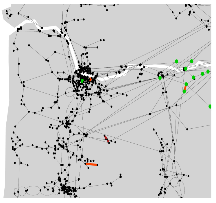
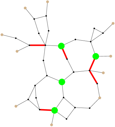
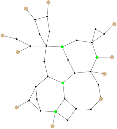
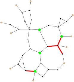
A possible failure scenario is illustrated in Fig. 1 using as example the U.S. Pacific Northwest regional grid data (2866 lines, 2209 buses, 176 generators and 18 wind sources), where lines highlighted in red are jeopardized (flow becomes too high) with unacceptably high probability by fluctuating wind resources positioned along the Columbia river basin (green dots marking existing wind farms). We propose a solution that requires, as the only additional investment, accurate wind forecasts; but no change in machinery or significant operational procedures. Instead, we propose an intelligent way to modify the optimization approach so as to mitigate risk; the approach is implementable as an efficient algorithm that solves realistic examples with thousands of buses and lines (such as the U.S. Pacific Northwest case) in a matter of seconds, and is thus only slightly slower than standard economic dispatch methods even on large-scale caes.
Maintaining line flows within their prescribed limits arises as a paramount operational criterion toward grid stability. In the context of incorporating renewables into generation, a challenge emerges because a nominally safe way of operating a grid may become unsafe – should an unpredictable (but persistent) change in renewable output occur, the resulting power flows may cause a line to persistently exceed its rating. It is natural to assess the risk of such an event in terms of probabilities, because of the non-deterministic behavior of e.g. wind; thus in our proposed operational solution we will rely on techniques involving both mathematical optimization and risk analysis.
When considering a system under stochastic risk, an extremely large variety of events that could pose danger might emerge. Recent works [17, 18, 1] suggest that focusing on instantons, or most-likely (dangerous) events, provides a practicable route to risk control and assessment. However, there may be far too many comparably probable instantons, and furthermore, identifying such events does not answer the question of what to do about them. In other words, we need a computationally efficient methodology that not only identifies dangerous, relatively probable events, but also mitigates them.
This paper suggests a new approach for handling the two challenges, that is to say, searching for the most probable realizations of line overloads under renewable generation, and correcting such situations through control actions, simultaneously and efficiently in one step. Our approach relies on methodologies recently developed in the optimization literature and known under the name of ”Chance-Constrained” (CC) optimization [41]. Broadly speaking, CC optimization problems are optimization problems involving stochastic quantities, where constraints state that the probability of a certain random event is kept smaller than a target value.
To address these goals, we propose an enhancement of the standard OPF to be used in the economic dispatch of the controllable generators. We model each bus that houses a power source subject to randomness to include a random power injection, and reformulate the standard OPF in order to account for this uncertainty. The formulation minimizes the average cost of generation over the random power injections, while specifying a mechanism by which (standard, i.e. controllable) generators compensate in real-time for renewable power fluctuations; at the same time guaranteeing low probability that any line will exceed its rating. This last constraint is naturally formulated as a chance constraint – we term out approach Chance-Constrained OPF, or CC-OPF.
This paper is organized as follows. In Section 1 we motivate and present the various mathematical models used to describe how the grid operates, as well as our proposed methodology. We explain how to solve the models in Section 2. We then present, in Section 3 a number of examples to demonstrate the speed and usefulness of our approach. Section 4 summarizes the results and discusses the path forward.
1 Formulating Chance-Constrained Optimum Power Flow Models
1.1 Transmission Grids: Controls and Limits
The power systems we consider in this paper are transmission grids which operate at high voltages so as to convey power economically, with minimal losses, over large distances. This is to be contrasted with distribution systems; typically residential, lower voltage grids used to provide power to individual consumers. From the point of view of wind-power generation, smooth operation of transmission systems is key since reliable wind sources are frequently located far away from consumption.
Transmission systems balance consumption/load and generation using a complex strategy that spans three different time scales (see e.g. [4]). At any point in time, generators produce power at a previously computed base level. Power is generated (and transmitted) in the Alternating Current (AC) form. An essential ingredient toward stability of the overall grid is that all generators operate at a common frequency. In real time, changes in loads are registered at generators through (opposite) changes in frequency. A good example is that where there is an overall load increase. In that case generators will marginally slow down – frequency will start to drop. Then the so-called primary frequency control, normally implemented on gas and hydro plans with so-called “governor” capability will react so as to stop frequency drift (large coal and nuclear units are normally kept on a time constant output). This is achieved by having each responding generator convey more power to the system, proportionally to the frequency change sensed. (In North America the proportionality coefficient is normally set to 5% of the generator capacity for 0.5Hz deviation from the nominal frequency of 60Hz.) This reaction is swift and local, leading to stabilization of frequency across the system, however not necessarily at the nominal 60Hz value. The task of the secondary, or Automatic Gain Control (AGC), is to adjust the common frequency mismatch and thus to restore the overall balance between generation and consumption, typically in a matter of minutes. Only some of the generators in a local area may be involved in this step. The final component in the strategy is the tertiary level of control, executed via the OPF algorithm, typically run as frequently as every fifteen minutes (to one hour), and using estimates for loads during the next time window, where base (controllable) generator outputs are reset. This is not an automatic step in the sense that a computation is performed to set these generator levels; the computation takes into account not only load levels but also other parameters of importance, such as line transmission levels. Tertiary control computation, which is in the center of this paper, thus represents the shortest time scale where actual off-line and network wide (in contrast to automatic primary and secondary controls of frequency) optimal computations are employed. The three levels are not the only control actions used to operate a transmission system. Advancing further in the time scale, OPF is followed by the so-called Unit Commitment (UC) computation, which schedules the switching on and off of large generation units on the scale of hours or even days.
A critical design consideration at each of the three control levels is that of maintaining “stability” of the grid. The most important ingredient toward stable operation is synchrony – ultimately, all the generators of the network should stabilize thus locking, after a perturbation followed by a seconds-short transient, at the same frequency. Failure to do so not only proves inefficient but, worse, it threatens the integrity of the grid, ultimately forcing generators to shut down for protective reasons – thus, potentially, causing a large, sudden change in power flow patterns (which may exceed equipment limits, see below) and possibly also an unrecoverable generation shortage. A second stability goal is that of maintaining large voltages. This is conducive to efficiency; lower voltage levels cause as a byproduct more generation (to meet the loads) and larger current values. Not only is this combination inefficient, but in an extreme case it may make impossible to meet existing loads (so-called “voltage collapse” is a manifestation of this problem). The third stability goal, from an operational perspective, is that of maintaining (line) power flows within established bounds. In long transmission lines, a large flow value will cause excessive voltage drop (an undesirable outcome as discussed). On a comparatively shorter line, an excessively large power flow across the line will increase the line temperature to the point that the line sags, and potentially arcs or trips due to a physical contact. For each line there is a given parameter, the line rating (or limit) which upper bounds flow level during satisfactory operation.
Of the three “stability” criteria described above, the first two (maintaining synchrony and voltage) are a concern only in a truly nonlinear regime which under normal circumstances occur rarely. Thus, we focus on the third – observing line limits.
1.2 OPF – Standard Generation Dispatch (tertiary control)
OPF is a key underlying algorithm in power engineering; see the review in [33] and e.g. [35, 4]. The task of OPF, usually executed off-line at periodic intervals, is to reset generator output levels over a control area of the transmission grid, for example over the Bonneville Power Administration (BPA) grid shown in Fig. 1. In order to describe OPF we will employ power engineering terms such “bus” to refer to a graph-theoretic vertex and “line” to refer to an edge. The set of all buses will be denoted by , the set of lines, and the set of buses that house generators, . We let . A line joining buses and is denoted by indicating an arbitrary but fixed ordering. We assume that the underlying graph is connected, without loss of generality.
The generic OPF problem can be stated as follows:
-
•
The goal is to determine the vector , where for , is the output of generator , so as to of minimize an objective function . This function is, usually, a convex, separable quadratic function of :
where each is convex quadratic.
-
•
The problem is endowed by three types of constraints: power flow, line limit and generation bound constraints.
Among the constraints, the simplest are the generation bounds, which are box constraints on the individual . The thermal line limits place an upper bound on the power flows in each line. We will return to these constraints later on; they are related to the physics model describing the transport of power in the given network, which is described by the (critical) power flow constraints. In the most general form, these are simply Kirchoff’s circuit laws stated in terms of voltages (potentials) and power flows. In this context, for each bus its voltage is defined as , where and are the voltage magnitude and phase angle at bus . Voltages can be used to derive expression for other physical quantities, such as current and, in particular, power, obtaining in the simplest case a system of quadratic equations on the voltage real and imaginary coordinates. See e.g. [35, 4].
The AC power flow equations can constitute an obstacle to solvability of OPF (from a technical standpoint, they give rise to nonconvexities). In transmission system analysis a linearized version of the power flow equations is commonly used, the so-called “DC-approximation”. In this approximation (a) all voltages are assumed fixed and re-scaled to unity; (b) phase differences between neighboring nodes are assumed small, , (c) thermal losses are ignored (reactance dominates resistance for all lines). Then, the (real) power flow over line , with line susceptance is related linearly to the respective phase difference,
| (1) |
Suppose, for convenience of notation, that we extend the vector to include an entry for every bus with the proviso that whenever . Likewise, denote by the vector of (possibly zero) demands and by the vector of phase angles. Then, a vector of power flows is feasible if and only if
| (2) |
and in view of equation (1), this can be restated as
| (3) |
In matrix form this equation can be rewritten as follows:
| (4) |
where the matrix is a weighted-Laplacian defined as follows:
| (8) |
For future reference, we state some well known properties of Laplacians and the power flow system (4).
Lemma 1.1.
The sum of rows of is zero and under the connectedness assumption for the underlying graph the rank of equals . Thus system (4) is feasible in if and only if
| (10) |
In other words: under the DC model the power flow Eqs. (4) are feasible precisely when total generation equals total demand. Moreover, if Eqs. (4) are feasible, then for any index there is a solution with .
In summary, the standard DC-formulation OPF problem can be stated as the following constrained optimization problem:
| (11) | |||||
| (12) | |||||
| (13) | |||||
| (14) |
Note that the quantities can be used to enforce the convention for each ; if then are lower and upper generation bounds which are generator-specific. Here, Constraint (14) is the line limit constraint for ; represents the line limit (typically a thermal limit), which is assumed to be strictly enforced in constraint (14). This conservative condition will be relaxed in the following.
Problem (11) is a convex quadratic program, easily solved using modern optimization tools. The vector of demands is fixed in this problem and is obtained through estimation. In practice, however, demand will fluctuate around ; generators then respond by adjusting their output (from the OPF-computed quantities) proportionally to the overall fluctuation as will be discussed below.
The scheme (11) works well in current practice, as demands do not substantially fluctuate on the time scale for which OPF applies. Thus the standard practice of solving (11) in the feasibility domain defined by Eq. (12),(8),(13),(14), using demand forecasts based on historical data (and ignoring fluctuations) has produced a very reliable result - generation re-dispatch covering a span of fifteen minutes to an hour, depending on the system.
1.3 Chance constrained OPF: motivation
To motivate the problem we outline how generator output is modulated, in real time, in response to fluctuations of demand. Suppose we have computed, using OPF, the output for each generator assuming constant demands . Let be the vector of real-time demands at time . Then so-called “frequency control”, or more properly, primary and secondary controls in combination that we will also call in the sequel “affine” control, will reset generator outputs to quantities according to the following scheme
| (15) |
In this equation, the quantities are fixed and satisfy
Thus, from (15) we obtain
from Eq. (10), in other words, demands are met. The quantities are generator dependent but essentially chosen far in advance and without regard to short-term demand forecasts.
Thus, in effect, generator outputs are set in hierarchical fashion (first OPF, with adjustments as per (15) which is furthermore risk-unaware. This scheme has worked in the past because of the slow time scales of change in uncontrolled resources (mainly loads). That is to say, frequency control and load changes are well-separated. Note that a large error in the forecast or an under-estimation of possible for the next –e.g., fifteen minute– period may lead to an operational problem in standard OPF (see e.g. the discussions in [14, 37]) because even though the vector is sufficient to meet demands, the phase angles computed from
give rise to real-time power flows
that violate constraints (14). In fact, even the generator constraints (13) may fail to hold. This has not been considered a handicap, however, simply because line trips due to overloading as a result of OPF-directed generator dispatch were (and still are) rare, primarily because the deviations will be small in the time scale of interest. In effect, the risk-unaware approach that assumes constant demands in solving the OPF problem has worked well.
This perspective changes when renewable power sources such as wind are incorporated. We assume that a subset of the buses holds uncertain power sources (wind farms); for each , write the amount of power generated by source at time as , where is the forecast output of farm in the time period of interest. For ease of exposition, we will assume in what follows that refers to the set of buses holding controllable generators, i.e. . Renewable generation can be seamlessly incorporated into the OPF formulation (11)-(14) by simply setting for each . Assuming constant demands but fluctuating renewable generation, the application of the frequency control yields the following analogue to (15):
| (16) |
e.g. if , that is to say, there is a net increase in wind output, then (controllable) generator output will proportionally decrease.
Eq. (16) describes how generation will adjust to wind changes, under current power engineering practice. The hazard embodied in this relationship is that the quantities can be large resulting in sudden and large changes in power flows, large enough to substantially overload power lines and thereby cause their tripping, a highly undesirable feature that compromises grid stability. The risk of such overloads can be expected to increase (see [19]); this is due to a projected increase of renewable penetration in the future, accompanied by the decreasing gap between normal operation and limits set by line capacities. Lowering of the TL limits (the quantities in Eqs. (14)) can succeed in deterministically preventing overloads, but it also forces excessively conservative choices of the generation re-dispatch, potentially causing extreme volatility of the electricity markets. See e.g. the discussion in [47] on abnormal price fluctuations in markets that are heavily reliant on renewables.
1.4 Using chance constraints
Power lines do not fail (i.e., trip) instantly when their flow thermal limits are exceeded. A line carrying flow that exceeds the line’s thermal limit will gradually heat up and possibly sag, increasing the probability of an arc (short circuit) or even a contact with neighboring lines, with ground, with vegetation or some other object. Each of these events will result in a trip. The precise process is extremely difficult to calibrate (this would require, among other factors, an accurate representation of wind strength and direction in the proximity of the line)111We refer the reader to [26] for discussions of line tripping during the 2003 Northeast U.S.-Canada cascading failure.. Additionally, the rate at which a line overheats depends on its overload which may dynamically change (or even temporarily disappear) as flows adjust due to external factors; in our case fluctuations in renewable outputs. What can be stated with certainty is that the longer a line stays overheated, the higher the probability that it will trip – to put it differently, if a line remains overheated long enough, then, after a span possibly measured in minutes, it will trip. In summary, (thermal) tripping of a line is primarily governed by the historical pattern of the overloads experienced by the line, and thus it may be influenced by the status of other lines (implicitly, via changes in power flows); further, exogenous factors can augment the impact of overloads.
Even though an exact representation of line tripping seems difficult, we can however state a practicable alternative. Ideally, we would use a constraint of the form “for each line, the fraction of the time that it exceeds its limit within a certain time window is small”. Direct implementation of this constraint would require resolving dynamics of the grid over the generator dispatch time window of interest. To avoid this complication, we propose instead the following static proxy of this ideal model, a chance constraint: “we will require that the probability that a given line will exceed its limit is small”.
To formalize this notion, we assume:
-
W.1.
For each , the (stochastic) amount of power generated by source is of the form , where
-
W.2.
is constant, assumed known from the forecast, and is a zero mean independent random variable with known standard deviation .
Here and in what follows, we use bold face to indicate uncertain quantities. Let be the flow on a given line , and let be small. The chance constraint for line , is:
| (17) |
One could alternatively use
| (18) |
which is less conservative than (17). If (18) holds then so does (17), and if the latter holds then . However, (17) proves more tractable, and moreover we are interested in the regime where is fairly small; thus we estimate that there is small practical difference between the two constraints; this will be verified by our numerical experiments. Likewise, for a generator we will require that
| (19) |
The parameter will be chosen extremely small, so that for all practical purposes the generator’s will be guaranteed to stay within its bounds.
Chance constraints [45], [15], [38] are but one possible methodology for handling uncertain data in optimization. Broadly speaking, this methodology fits within the general field of stochastic optimization. Constraint (17) can be viewed as a “value-at-risk” statement; the closely-related “conditional value at risk” concept provides a (convex) alternative, which roughly stated constrains the expected overload of a line to remain small, conditional on there being an overload (see [41] for definitions and details). Even though alternate models are possible, we would would argue that our chance constrained approach is reasonable (in fact: compelling) in view of the nature of the line tripping process we discussed above.
[50] considers the standard OPF problem under stochastic demands, and describes a method that computes fixed generator output levels to be used throughout the period of interest, independent of demand levels. In order to handle variations in demand, [50] instead relies on the concept of a slack bus. A slack bus is a fixed node that is assumed to compensate for all generation/demand mismatches – when demand exceeds generation the slack bus injects the shortfall, and when demand is smaller than generation the slack bus absorbs the generation excess. A vector of generations is acceptable if the probability that each system component operates within acceptable bounds is high – this is a chance constraint. To tackle this problem [50] proposes a simulation-based local optimization system consisting of an outer loop used to assess the validity of a control (and estimate its gradient) together with an inner loop that seeks to improve the control. Experiments are presented using a 5-bus and a 30-bus example. The approach in [50], though universal (i.e., applicable to any type of exogenous distribution), requires a number of technical assumptions and elaborations to guarantee convergence and feasibility and appears to entail a very high computational cost.
Another related study [46] describes a security constrained optimization for reserve scheduling with fluctuating wind generation. Security constraints are represented via a set of outage scenarios. Finite time optimization horizon (24 steps, one per hour) is considered. As in our study, the standard DC power flow approach is adopted and no load uncertainty is considered. However, in a contrast with our setting wind generation in [46] is assumed localized (located at a single bus) in a small, 30 bus network. Under the assumption that the probability distribution function of the aggregated wind resources is known, the cost of generation over the time horizon is optimized under the chance constrains for line overloads and generation limits. The stochastic optimization is tackled in [46] via transformation to a convex optimization on the expense of a number of approximations, including scenario approach to the wind forecast, look-up table modeling of the security constraints, and a heuristic scheme for a bilinear descent iteration, with no convergence to global optimum of the nonlinear problem guaranteed.
Chance constrained optimization has also been discussed recently in relation to the Unit Commitment problem, which concerns discrete-time planning for operation of large generation units on the scale of hours-to-months, so as to account for the long-term wind-farm generation uncertainty [42, 48, 51].
1.5 Uncertain power sources
The physical assumptions behind our model of uncertainty are as follows. Independence of fluctuations at different sites is due to the fact that the wind farms are sufficiently far away from each other. For the typical OPF time span of 15 min and typical wind speed of , fluctuations of wind at the farms more than apart are not correlated. We also rely on the assumption that transformations from wind to power at different wind farms is not correlated.
To formulate and calibrate our models, we make simplifying assumptions that are approximately consistent with our general physics understanding of fluctuations in atmospheric turbulence; in particular we assume Gaussianity of 222Correlations of velocity within the correlation time of 15 min, roughly equivalent to the time span between the two consecutive OPF, are approximately Gaussian. The assumption is not perfect, in particular because it ignores significant up and down ramps possibly extending tails of the distribution in the regime of really large deviations.. We will also assume that only a standard weather forecast (coarse-grained on minutes and kilometers) is available, and no systematic spillage of wind in its transformation to power is applied333See [19], for some empirical validation..
There is an additional and purely computational reason for the Gaussian assumption, which is that under this assumption chance constraint (17) can be captured using in an optimization framework that proves particularly computationally practicable. We will also consider a data-robust version of our chance-constrained problem where the parameters for the Gaussian distributions are assumed unknown, but lying in a window. This allows both for parameter mis-estimation and for model error, that is to say the implicit approximation of non-Gaussian distributions with Gaussians; our approach, detailed in Section 2.4, remains computationally sound in this robust setting.
Other fitting distributions considered in the wind-modeling literature, e.g. Weibull distributions and logistic distributions [11, 32], will be discussed later in the text as well 444Note that the fitting approach of [11, 32] does not differentiate between typical and atypical events and assumes that the main body and the tail should be modeled using a simple distribution with only one or two fitting parameters. Generally this assumption is not justified as the physical origin of the typical and anomalous contributions of the wind, contributing to the main body and the tail of the distribution respectively, are rather different. Gaussian fit (of the tail) – or more accurately, faster than exponential decay of probability in the tail for relatively short-time (under one hour) forecast – would be reasonably consistent with phenomenological modeling of turbulence generating these fluctuations.. In particular, we will demonstrate on out-of-sample tests that the computationally advantageous Gaussian modeling of uncertainty allows as well to model effects of other distributions.
1.6 Affine Control
Since the power injections at each bus are fluctuating, we need a control to ensure that generation is equal to demand at all times within the time interval between two consecutive OPFs. We term the joint result of the primary frequency control and secondary frequency control the affine control. The term will intrinsically assume that all governors involved in the controls respond to fluctuations in the generalized load (actual demand which is assumed frozen minus stochastic wind resources) in a proportional way, however with possibly different proportionality coefficients. Then, the random variable dependent version of Eq. (16) becomes
| (20) |
Here the quantities and are design variables satisfying (among other constraints) . Notice that we do not set any to a standard (fixed) value, but instead leave the optimization to decide the optimal value. (In some cases it may even be advantageous to allow negative but we decided not to consider such a drastic change of current policy in this study.) The generator output combines a fixed term and a term which varies with wind, . Observe that , that is, the total power generated equals the average production of the generators minus any additional wind power above the average case.
This affine control scheme creates the possibility of requiring a generator to produce power beyond its limits. With unbounded wind, this possibility is inevitable, though we can restrict it to occur with arbitrarily small probability, which we will do with additional chance constraints for all controllable generators, ,
| (21) |
1.7 CC-OPF: Brief Discussion of Solution Methodology
Our methodology applies and develops general ideas of [41] to the power engineering setting of generation re-dispatch under uncertainty. In Section 2.1 we will provide a generic formulation of our chance-constrained OPF problem that is valid under the assumption of linear power flow laws and statistical independence of wind fluctuations at different sites, while using control law (20) to specify standard generation response to wind fluctuations. Under the additional assumption of Gaussianity, this generic formulation is reduced to a specific deterministic optimization problem of Section 2.2. Moreover this deterministic optimization over and is a convex optimization problem, more precisely, a Second-Order Cone Program (SOCP) [12, 27], allowing an efficient computational implementation discussed in detail in Section 2.3. We will term this SOCP, which assumes point estimates for the wind distributions, the nominal problem. As indicated above, we also discuss how the SOCP formulation can be extended to account for data-related uncertainty in the parameters of the Gaussian distributions in Section 2.4, obtaining a robust version of the chance-constrained optimization problem.
Let us emphasize that many of our assumptions leading to the computational efficient nominal formulation are not restrictive and allow natural generalizations. In particular, using techniques from [41], it is possible to relax the phenomenologically reasonable but approximately validated assumption of wind source Gaussianity (validated according to actual measurements of wind, see [11, 32] and references therein). For example, using only the mean and variance of output at each wind farm, one can use Chebyshev’s inequality to obtain a similar though more conservative formulation. And following [41] we can also obtain convex approximations to (17) which are tighter than Chebyshev’s inequality, for a large number of empirical distributions discussed in the literature. The data-robust version of our algorithm provides a methodologically sound (and computationally efficient) means to protect against data and model errors; moreover we will perform (below) out-of-sample experiments involving the controls computed with the nominal approach; first to investigate the effect of parameter estimation errors in the Gaussian case, and, second, to gauge the impact of non-Gaussian wind distributions.
2 Solving the Models
2.1 Chance-constrained optimal power flow: formal expression
Following the W.1 and W.2 notations, Eqs. (20) explain the affine control, given that the are decision variables in our CC-OPF, additional to the standard decision variables already used in the standard OPF (11). For write , thereby obtaining a vector . Likewise, extend and to vectors in by writing whenever .
Definition. We say that the pair is viable if the generator outputs under control law (20), together with the uncertain outputs, always exactly match total demand.
The following simple result characterizes this condition as well as other basic properties of the affine control. Here and below, is the vector of all 1’s.
Lemma 2.1.
Under the control law (20) the net output of bus equals
| (22) |
and thus the (stochastic) power flow equations can be written as
| (23) |
Consequently, the pair is viable if and only if
| (24) |
Proof. Eq. (22) follows by definition of the , , vectors and the control law. Thus Eq. (23) holds. By Lemma 1.1 from Eq. (23) one gets that is viable iff
| (25) | |||||
since by construction .
Remark. Equation (24) can be interpreted as stating the condition that expected total generation must equal total demand; however the Lemma contains a rigorous proof of this fact.
As remarked before, any matrix obtained by striking out the same column and row of is invertible. For convenience of notation we will assume that bus is neither a generator nor a wind farm bus, that is to say, , and we denote by the submatrix obtained from by removing row and column , and write
| (28) |
Further, by Lemma 1.1 we can assume without loss of generality that . The following simple result will be used in the sequel.
Lemma 2.2.
Suppose the pair is viable. Then under the control law (20) a vector of (stochastic) phase angles is
| (29) | |||||
| (30) |
As a consequence,
| (31) |
and given any line ,
| (32) |
Furthermore, each quantity or is an affine function of the random variables .
Proof. For convenience we rewrite system (23): Since is viable, this system is always feasible, and since the sum of rows of is zero, its last row is redundant. Therefore Eq. (29) follows since , and Eq. (31) holds since has zero mean. Since for all Eq. (32) holds. From this fact and Eq. (29) it follows that and are affine functions of .
Using this result we can now give an initial formulation to our chance-constrained problem; with discussion following.
| (33) | |||
| (34) | |||
| (35) | |||
| (36) | |||
| for all lines : | |||
| (37) | |||
| (38) | |||
| for all generators : | |||
| (39) |
The variables in this formulation are and . Constraint (34) simply states basic conditions needed by the affine control. Constraint (35) is (24). Constraints (36), (37) and (38) express our chance constraint, in view of Lemma 2.2.
The objective function is the expected cost incurred by the stochastic generation vector
over the varying wind power output . In standard power engineering practice generation cost is convex, quadratic and separable, i.e. for any vector , where each is convex quadratic. Note that for any we have
from which we obtain, since the have zero mean,
where “var” denotes variance and . It follows that the objective function can be written as
| (40) |
where for all . Consequently the objective function is convex quadratic, as a function of and .
The above formulation is the formal statement for our optimization problem. Even though its objective is convex in cases of interest, the formulation is not in a form that can be readily exploited by standard optimization algorithms. Below we will provide an efficient approach to solve relevant classes of problems with the above form; prior to that we need a technical result. We will employ the following notation:
-
•
For , the variance of is denoted by .
-
•
For let denote the entry of the matrix given above, that is to say,
(43) -
•
Given , for write
(46)
Lemma 2.3.
Assume that the are independent random variables. Given , for any line ,
| (47) |
Proof. Using and eq. (29) we have that
| (48) | |||||
| (49) | |||||
| (50) |
since by convention for any . The result now follows.
Remark. Lemma 2.3 holds for any distribution of the so long as independence is assumed. Similar results are easily obtained for higher-order moments of the .
2.2 Formulating the chance-constrained problem as a conic program
In deriving the above formulation (33)-(39) for CC-OPF we assumed that the random variables have zero mean. To obtain an efficient solution procedure we will additionally assume that they are (a) pairwise independent and (b) normally distributed. These assumptions were justified in Section 1.5. Under the assumptions, however, since the are affine functions of the (because the are, by eq. (29)), it turns out that there is a simple restatement of the chance-constraints (37), (38) and (39) in a computationally practicable form. See [41] for a general treatment of linear inequalities with stochastic coefficients. For any real we write , where is the cdf of a standard normally distributed random variable.
Lemma 2.4.
Let , be viable. Assume that the are normally distributed and independent. Then:
For any line , and if and only if
| (51) |
where as before and
.
For any generator , and iff
| (52) |
Proof. By Lemma 2.2, is an affine function of the ; under the assumption it follows that is itself normally distributed. Thus, iff
| (53) |
and similarly, iff
| (54) |
Lemma 2.2 gives while by Lemma 2.3,
. Substituting these values into (53) and
(54) yields (51). The proof of (52) is similar.
Remarks Eq. (51) highlights the difference between e.g. our chance constraint for lines, which requires that and that , and the stricter requirement that which amounts to
| (55) |
Unlike our requirement, which is captured by (51),
the stricter condition (55) does not admit a compact statement.
We can now present a formulation of our chance-constrained optimization as a convex optimization problem, on variables and :
| (56) | |||||
| (57) | |||||
| (58) | |||||
| (59) | |||||
| (60) | |||||
| (61) | |||||
| (62) | |||||
| (63) | |||||
| (64) |
In this formulation, the variables are auxiliary and introduced to facilitate the discussion below – since without loss of generality (62) will hold as an equality. Constraints (62), (63) and (64) are second-order cone inequalities [12]. A problem of the above form is solvable in polynomial time using well-known methods of convex optimization; several commercial software tools such as Cplex [20], Gurobi [31], Mosek [39] and others are available. Constraint (57) is equivalent to (as we did in (46)), however can be seen to be totally dense, whereas is very sparse for typical grids. Constraint (62) can be relatively dense – the sum has a term for each farm. However as a percentage of the total number of buses this can be expected to be small.
2.3 Solving the conic program
Even though optimization theory guarantees that the above problem is efficiently solvable, experimental testing shows that in the case of large grids (thousands of lines) the problem proves challenging. For example, in the Polish 2003-2004 winter peak case555Available with MATPOWER [52], we have buses, lines and wind farms, and Cplex [20] reports (after pre-solving) variables and constraints, of which are conic. On this problem, a recent version of Cplex on a (current) 8-core workstation ran for seconds (on 16 parallel threads, making use of “hyperthreading”) and was unable to produce a feasible solution. On the same problem Gurobi reported “numerical trouble” after 31.1 cpu seconds, and stopped.
In fact, all of the commercial solvers [20, 31, 39] we experimented with reported numerical difficulties with problems of this size. Anecdotal evidence indicates that the primary cause for these difficulties is not simply the size, but also to a large degree numerics in particular poor conditioning due to the entries in the matrix . These are susceptances, which are inverses of reactances, and often take values in a wide range.
To address this issue we implemented an effective algorithm for solving problem (56)-(64). For brevity we will focus on constraints (62) ((63) and (64) are similarly handled). For a line define
Constraint (62) can thus be written as . For completeness, we state the following result:
Lemma 2.5.
Constraint (62) is equivalent to the infinite set of linear inequalities
| (65) |
Constraints (65) express the outer envelope of the set described by (62) [12]. Any vector which satisfies (62) (for a given choice of ) is guaranteed to satisfy (65). Thus a a finite subset of the inequalities (65), used instead of (62), will give rise to a relaxation of the optimization problem and thus a lower bound on the optimal objective value. Given Lemma 2.5 there are two ways to proceed, both motivated by the observation that at , the most constraint inequality from among the set (65) is that obtained by choosing .
First, one can use inequalities (65) as cutting-planes in the context of the ellipsoid method [30], obtaining a polynomial-time algorithm. A different way to proceed yields a numerically practicable algorithm. For brevity, we will omit treatment of the generator conic constraints (63), (64) (which are similarly handled). Denote by the objective function in Eq. (56).
Procedure 2.6.
CUTTING-PLANE ALGORITHM
Initialization: The linear “master” system is defined to include constraints (57)-(61).
Iterate:
(1) Solve . Let be an optimal solution.
(2) If all conic constraints are satisfied up to numerical
tolerance by
, Stop.
(3) If all chance constraints are satisfied up to numerical
tolerance by , Stop.
(4) Otherwise, add to the master system the outer inequality (65)
arising from that constraint (62) which is most violated.
As the algorithm iterates the master system represents a valid relaxation of the conic program (57)-(62); thus the objective value of the solution computed in Step 1 is a valid lower bound on the value of problem. Each problem solved in Step 1 is a linearly constrained, convex quadratic program. Computational experiments involving large-scale realistic cases show that the algorithm is robust and rapidly converges to an optimum.
Note that Step 3 is not redundant. The stopping condition in Step 2 may fail because the variance estimates are incorrect (too small), nevertheless the pair may already satisfy the chance constraints. Checking that it does, for a given line , is straightforward since the flow is normally distributed (as noted in Lemma 2.4) and its mean and variance can be directly computed from .
In our implementation termination is declared in Step 2 or Sep 3 when the corresponding constraint violation is less than . Table LABEL:larger displays typical performance of the cutting-plane algorithm on (comparatively more difficult) large problem instances. In the Table, ’Polish1’-’Polish3’ are the three Polish cases included in MATPOWER [52] (in Polish1 we increased loads by ). All Polish cases have uniform random costs on [0.5, 2.0] for each generator and ten arbitrarily chosen wind sources. The average wind power penetration for the four cases is 8.8%, 3.0%, 1.9%, and 1.5%. ’Iterations’ is the number of linearly-constrained subproblems solved before the algorithm converges. ’Barrier iterations’ is the total number of iterations of the barrier algorithm in CPLEX over all subproblems, and ’Time’ is the total (wallclock) time required by the algorithm. For each case, line tolerances are set to two standard deviations and generator tolerances three standard deviations. These instances all prove unsolvable if directly tackled by CPLEX or Gurobi.
| Case | Buses | Generators | Lines | Time (s) | Iterations | Barrier iterations |
|---|---|---|---|---|---|---|
| BPA | 2209 | 176 | 2866 | 5.51 | 2 | 256 |
| Polish1 | 2383 | 327 | 2896 | 13.64 | 13 | 535 |
| Polish2 | 2746 | 388 | 3514 | 30.16 | 25 | 1431 |
| Polish3 | 3120 | 349 | 3693 | 25.45 | 23 | 508 |
Table LABEL:detailed provides additional, typical numerical performance for the cutting-plane algorithm on an instance of the Polish grid model. Each row of Table LABEL:detailed shows that maximum relative error and objective value at the end of several iterations. The total run-time was 25 seconds. Note the “flatness” of the objective. This makes the problem nontrivial – the challenge is to find a feasible solution (with respect to the chance constraints); at the onset of the algorithm the computed solution is quite infeasible and it is this attribute that is quickly improved by the cutting-plane algorithm.
| Iteration | Max rel. error | Objective |
|---|---|---|
| 1 | 1.2e-1 | 7.0933e6 |
| 4 | 1.3e-3 | 7.0934e6 |
| 7 | 1.9e-3 | 7.0934e6 |
| 10 | 1.0e-4 | 7.0964e6 |
| 12 | 8.9e-7 | 7.0965e6 |
We note the (typical) small number of iterations needed to attain numerical convergence. Thus at termination only a very small number of conic constraints (62) have been incorporated into the master system. This validates the expectation that only a small fraction of the conic constraints in CC-OPF are active at optimality. The cutting-plane algorithm can be viewed as a procedure that opportunistically discovers these constraints.
2.4 Data-robust chance constraints
Above we developed a formulation for our chance-constrained OPF problem as the conic program (56)-(64). This approach assumed exact estimates for the mean and the variance of each wind source . In practice however the estimates at hand might be imprecise666In particular since they would effectively be computed in real time.; consequently jeopardizing the usefulness of our conic program, henceforth termed the nominal chance-constrained problem. In particular, the performance of the control computed by the conic program might conceivably be sensitive to even small changes in the data. We will deal with this issue in two complimentary ways.
2.4.1 Out-of-sample analysis
Our first approach is the out-of-sample tests, implemented experimentally in Section 3.7. We assume that the and have been mis-estimated and explore the robustness of the affine control with respect to the estimation errors. The experiments of Section 3.7 show that the degradation of the chance constraints is small when small data errors are experienced. This empirical observation has a rigorous explanation discussed below.
Our chance constraints are represented by convex inequalities, for example in the case of and we used e.g. (61) and (62). Suppose that we have solved the chance-constrained problem assuming (incorrect) expectations and variances (). Let and () be the exact (or realized) values. With some abuse of notation, we will write (resp., ) for the incorrect (exact) distribution. For a given line , write:
| (66) | |||
| (67) |
and similarly,
| (68) | |||
| (69) |
Using (68) and (69) we see that the “true” probability is that value such that
| (70) |
We wish to evaluate how much larger this (realized) value is compared with the target value which was the goal in the chance-constrained computation. We will do this assuming that the estimation errors are small, more precisely, there exist nonnegative constants and such that
| (71) |
Considering Eq. (70), we see that for data errors of a given magnitude, is maximized when and are maximized. Further, considering Eqs. (68) and Eqs. (69) we see that to first order , and that . From these two observations and eq. (70) we obtain
| (72) | |||||
The quantity in brackets in the right-hand side of (72) equals
| (73) | |||
| (74) | |||
| (75) |
Using (72) and (75) we obtain that , where the “O” notation “hides” solution-dependent constants.
2.4.2 Efficiently solvable data-robust formulations
As the preceding analysis makes clear, the constants and may need to be quite small, for example if the are small. We thus seek a better guarantee of robustness. This justifies our second approach discussed below – to develop a version of CC-OPF which is methodologically guaranteed to be insensitive to data errors. This approach puts CC-OPF within the scope of robust optimization; to be more precise we will be solving an ambiguous chance-constrained problem in the language of [25].
We will write each in the form , where the are point estimates of the and the are “errors” which are constrained to lie in some fixed set with . Likewise, we assume that there is a set including , such that each is of the form where the vector of errors belongs to . As an example for how to construct or , one can use the following set parameterized by values and :
| (76) |
This set was introduced in [6]. Another candidate is the ellipsoidal set
| (77) |
where is positive-definite and is a real; see [2], [28]. We can now formally proceed as follows:
Definitions. Let the estimates , and the sets and be given.
1. Let be the set of vectors of random variables such that for each pair and there is an element with coordinate-wise mean and variance .
2. A pair is called robust with respect to the pair , , if for each line
| (78) | |||
| (79) |
Our task will be to replace, in our optimization problem formulation, the chance constraint (17) with one asking for robustness as in Eqs. (78)-(79)777And likewise with the generator chance-constraints (63), (64).. If the uncertainty sets and consist of a single point estimate each, then we recover the nominal chance-constrained problem we discussed above. As or become larger, the robust approach becomes more insensitive to estimation errors, albeit at the cost of becoming more conservative. Thus, a reasonable balance should be attained by choosing and small but of positive measure, thereby preventing trivial sensitivity of the control to changes in the data.
To indicate our approach, we focus on one of the statements for our chance constraint for lines. Using Lemma 2.4, the robustness criterion (78) applied to a line requires
| (80) |
We can see that (80) consists of a (possibly infinite) set of convex constraints; thus the data-robust chance-constrained problem is a convex problem. However we need to exploit this fact in a computationally favorable manner. To motivate our approach, we will first show that a methodology based on traditional robust optimization techniques will (likely) not succeed at this task. We will then describe our method.
Considering the expression in brackets in the left-hand side of Eq. (80) we recall that depends on the uncertainty set , in fact we can write
| (81) |
where . Also, the are constants, and which is deterministic though dependent on our decision variables . In summary, constraint (80) can be rewritten as
| (82) | |||||
where is the vector with a +1 entry in position , a -1 entry in position and 0 elsewhere. Note that if in the left-hand side of (82) we ignore second term and the second term inside the square brackets, we obtain the nominal (i.e. non-robust) version of chance-constraint (78); see Eqs. (61), (62). A similar constraint is obtained from Eqs. (79).
Constraint (82) can be incorporated into a formulation provided we can appropriately represent the two maxima. Here, note that
| (83) |
is independent of all variables and can be solved beforehand for all lines ; when is of the form given above this is a linear programming problem and when the task amounts to finding a point in the boundary of an ellipsoid with normal parallel to a given vector and thus requires solving a linear system of equations. We will likewise define a quantity using instead of .
It is the second maximization that presents some challenges.
Lemma 2.7.
Suppose , and suppose a vector is given. Then
| s.t. | ||||
Proof sketch.
Since without loss of generality in the maximum we will have that for all . Strong linear programming duality now gives the result.
The use of linear programming duality as in Lemma 2.7 is key in the context of sets of the form . In the case of an ellipsoidal set as in (77) there is an analogue to Lemma 2.7 that instead uses the S-Lemma [12], [28]. In the standard robust optimization approach, Lemma 2.7 would be leveraged to produce a result of the following type:
Lemma 2.8.
Proof sketch. Without loss of generality at the optimum the and are chosen so as to minimize the left-hand side of (86) subject to all other variables held fixed, thereby obtaining the “min” in Lemma 2.7.
Lemma 2.8 points out the difficulty that the standard robust optimization approach would engender in the context of our problem. First, the number of constraints (86) and (87) is large: it equals and thus in the case of a large transmission system it could approach many tens of thousands (or more). Thus, even though we obtain a compact formulation (i.e., of polynomial size) it is likely to be proven too large for present-day solvers. But there is a second and more fundamental problem: constraint (86) is not convex. This is a significant methodological difficulty. A similar set of hurdles arises when using uncertainty sets .
2.4.3 Efficient solution of the data-robust problem using cutting planes
To derive an algorithm for the data-robust chance-constrained problem that (a) has some theoretical justification and (b) can prove numerically tractable, we return to inequality (82), and note that if we replace the set with a finite subset we obtain a valid relaxation. In other words
| (89) | |||
| (90) | |||
| (91) |
constitutes a valid relaxation of the chance constraints (61), (62) of the nominal formulation for each line for any given finite . This observation can be used to formally obtain a polynomial-time algorithm for the data-robust problem in the cases of interest. For a given let denote the expression inside the “max” in (91). For completeness, we state the following:
Lemma 2.9.
In the case of uncertainty sets of the form or the data-robust chance-constrained problem can be solved in polynomial time.
Proof. Suppose we are given quantities for each and for each line . Then as argued before, if is of the form or one can check in polynomial time whether . If the condition is violated for then trivially
| (92) |
is violated at . Since (92) is valid
for the data-robust chance-constrained problem (by convexity) the result follows
by relying on the ellipsoid method.
Lemma 2.9 describes a formally “good” algorithm. For computational purposes we instead would rely on a cutting-plane algorithm much like Algorithm 2.6, developed in Section 2.3 so as to handle the nominal chance-constrained problem. In the data-robust setting the algorithm is almost identical, except that given quantities for each and for each line we proceed as in the proof of Lemma 2.9 by finding a that proves most stringent for the pair and then add to the master formulation constraint (92). Details are left to the reader.
3 Experiments/Results
Here we will describe qualitative aspects of our affine control on small systems; in particular we focus on the contrast between standard OPF and nominal CC-OPF, on problematic features that can arise because of fluctuating wind sources and on out-of-sample testing of the CC-OPF solution, including the analysis of non-Gaussian distributions. Some of our tests involve the BPA grid and Polish Grid, which are large; we present additional set of tests to address the scalability of our solution methodology to the large cases.
3.1 Failure of standard OPF
Above (see Eq. (11)) we introduced the so-called standard OPF method for setting traditional generator output levels. When renewables are present, the natural extension of this approach would make use of some fixed estimate of output (e.g., mean output) and to handle fluctuations in renewable output through the same method used to deal with changes in load: ramping output of traditional generators up or down in proportion to the net increase or decrease in renewable output. This feature could seamlessly be handled using today’s control structure, with each generator’s output adjusted at a fixed (preset) rate. For the sake of simplicity, in the experiments below we assume that all ramping rates are equal.
Different assumptions on these fixed rates will likely produce different numerical results; however, this general approach entails an inherent weakness. The key point here is that mean generator output levels as well as in particular the ramping rates would be chosen without considering the stochastic nature of the renewable output levels. Our experiments are designed to highlight the limitations of this “risk-unaware” approach. In contrast, our CC-OPF produces control parameters (the and the ) that are risk-aware and, implicitly, also topology-aware – in the sense of network proximity to wind farms.
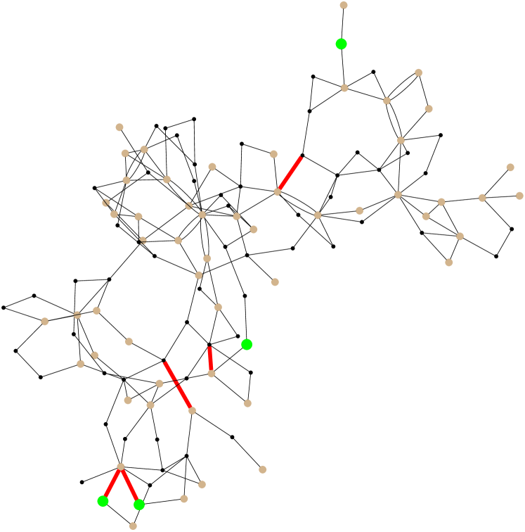
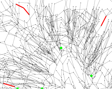
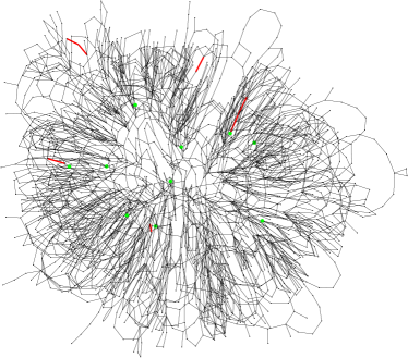
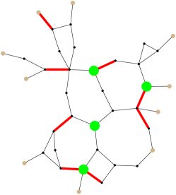
We first consider the IEEE 118-bus model with a quadratic cost function, and four sources of wind power added at arbitrary buses to meet 5% of demand in the case of average wind. The standard OPF solution is safely within the thermal capacity limits for all lines in the system. Then we account for fluctuations in wind assuming Gaussian and site-independent fluctuations with standard deviations set to 30% of the respective means. The results, which are shown in Fig. 2, illustrate that under standard OPF five lines (marked in red) frequently become overloaded, exceeding their limits 8% or more of the time. This situation translates into an unacceptably high risk of failure for any of the five red lines. This problem occurs for grids of all sizes; in Fig. 3 we show similar results on a 2746-bus Polish grid. In this case, after scaling up all loads by 10% to simulate a more highly stressed system, we added wind power to ten buses for a total of 2% penetration. The standard solution results in six lines exceeding their limits over 45% of the time, and in one line over 10% of the time. For an additional and similar experiment using the Polish grid see Section 3.8.
3.2 Cost of reliability under high wind penetration
The New York Times article “Wind Energy Bumps Into Power Grid’s Limits” [49] discusses how transmission line congestion has forced temporary shutdown of wind farms even during times of high wind. Our methodology suggests, as an alternative solution to curtailment of wind power, an appropriate reconfiguration of standard generators. If successful, this solution can use the available wind power without curtailment, and thus result in cheaper operating costs.
As a (crude) proxy for curtailment, we perform the following experiment, which considers different levels of renewable penetration. Here, the mean power outputs of the wind sources are kept in a fixed proportion to one another and proportionally scaled so as to vary total amount of penetration, and likewise with the standard deviations. First, we run our CC-OPF under a high penetration level. Second, we add a 10% buffer to the line limits and reduce wind penetration (i.e., curtail) so that under the standard OPF solution line overloads are reduced to an acceptable level. Assuming zero cost for wind power, the difference in cost for the high-penetration CC-OPF solution and the low-penetration standard solution are the savings produced by our model (generously, given the buffers).
For the 39-bus case, our CC-OPF solution is feasible under 30% of wind penetration, but the standard solution has 5 lines with excessive overloads, even when solved with the 10% buffer. Reducing the penetration to 5% relieves the lines, but more than quadruples(!) the cost over the CC-OPF solution. See Figure 4. Note that this approach does not only show the advantage of the CC-OPF over standard OPF but also provides a quantitative measure of the advantage, thus placing a well-defined price tag on reliability.
3.3 Non-locality
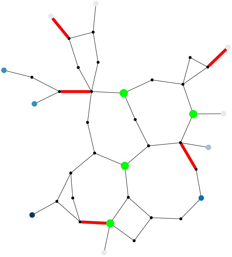
We have established that under fluctuating power generation, some lines may exceed their flow limits an unacceptable fraction of the time. Is there a simple solution to this problem, for instance, by carefully adjusting (a posteriori of the standard OPF) the outputs of the generators near the violated lines? The answer is no. Power systems exhibit significant non-local behavior. Consider Fig. 5. In this example, the major differences in generator outputs between the standard OPF solution and our CC-OPF model’s solution are not obviously associated with the different line violations. In general, it seems that it would be difficult to by-pass CC-OPF and make small local adjustments to relieve the stressed lines. On the positive side, even though CC-OPF is not local and requires a centralized computation, it is also only slightly more difficult than the standard OPF in terms of implementation.
3.4 Increasing penetration
Current planning for the power system in the United States calls for 30% of wind energy penetration by 2030 [23]. Investments necessary to achieve this ambitious target may focus on both software (improving operations) and hardware (building new lines, sub-stations, etc), with the former obviously representing a much less expensive and thus economically attractive option. Our CC-OPF solution contributes toward this option. A natural question that arises concerns the maximum level of penetration one can safely achieve by upgrading from the standard OPF to our CC-OPF.
To answer the question we consider the 39-bus New England system (from [52]) case with four wind generators added, and line flow limits scaled by .7 to simulate a heavily loaded system. The quadratic cost terms are set to rand(0,1) + .5. We fix the four wind generator average outputs in a ratio of 5/6/7/8 and standard deviations at 30% of the mean. We first solve our model using for each line and assuming zero wind power, and then increase total wind output until the optimization problem becomes infeasible. See Figure 6. This experiment illustrates that at least for the model considered, the 30% of wind penetration with rather strict probabilistic guarantees enforced by our CC-OPF may be feasible, but in fact lies rather close to the dangerous threshold. To push penetration beyond the threshold is impossible without upgrading lines and investing in other (not related to wind farms themselves) hardware.
3.5 Changing locations for wind farms
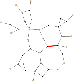
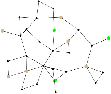
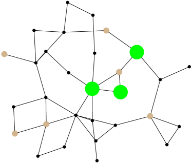
In this example we consider the effect of changing locations of wind farms. We take the MATPOWER 30-bus case with line capacities scaled by .75 and add three wind farms with average power output in a ratio of 2/3/4 and standard deviations at 30% of the average. Two choices of locations are shown in figure 7. The first remains feasible for penetration up to 10% while the second can withstand up to 55% penetration. This experiment shows that choosing location of the wind farms is critical for achieving the ambitious goal of high renewable penetration.
3.6 Reversal of line flows
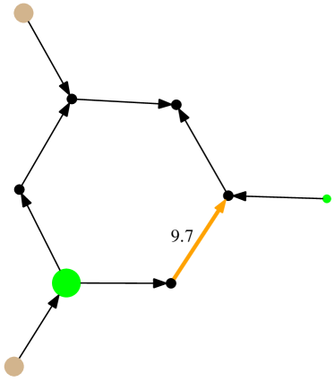
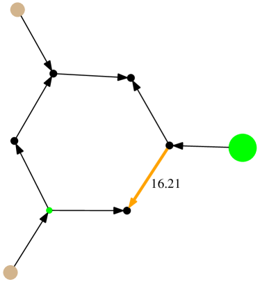
Here we consider the 9-bus case with two wind sources and 25% average penetration and standard deviations set to 30% of the average case and analyze the following two somewhat rare but still admissible wind configurations: (1) wind source (a) produces its average amount of power and source (b) three standard deviations below average; (2) the reverse of the case (1). This results in a substantial reversal of flow on a particular line shown in Figure 8. This example suggests that when evaluating and planning for grids with high-penetration of renewables one needs to be aware of potentially fast and significant structural rearrangements of power flows. Flow reversals and other qualitative changes of power flows, which are extremely rare in the grid of today, will become significantly much more frequent (typical) in the grid of tomorrow.
3.7 Out-of-sample tests
We now study the performance of the control computed using nominal CC-OPF when there are errors in the underlying distribution of wind power. We consider two types of errors: (1) the true distribution is non-Gaussian but our Gaussian fit is “close” in an appropriate sense, and (2) the true distribution is Gaussian but with different mean or standard deviation. The experiments in this section use as data set the BPA grid, which as noted before has 2209 buses and 2866 lines, and collected wind data; altogether constituting a realistic test-case.
We first consider the non-Gaussian case, using the following probability distributions, all with fatter tails than Gaussian: (1) Laplace, (2) logistic, (3) Weibull (three different shapes), (4) t location-scale with 2.5 degrees of freedom, (5) Cauchy. For the Laplace and logistic distributions, we simply match the mean and standard deviation. For the Weibull distribution, we consider shape parameters and choose the scale parameter to match the standard deviations. We then translate to match means. For the t distribution, we fix 2.5 degrees of freedom and then choose the location and scale to match mean and standard deviation. For the Cauchy distribution, we set the location parameter to the mean and choose the scale parameter so as to match the 95th percentiles.
We use our model and solve under the Gaussian assumption, seeking a solution which results in no line violations for cases within two standard deviations of the mean, i.e. a maximum of about 2.27% chance of exceeding the limit. We then perform Monte Carlo tests drawing from the above distributions to determine the actual rates of violation. See Figure 9. The worst-performer is the highly-asymmetric (and perhaps unreasonable) Weibull with shape parameter 1.2, which approximately doubles the desired maximum chance of overload. Somewhat surprisingly, the fat-tailed logistic and Student’s t distributions result in a maximum chance of overload significantly less than desired, suggesting that our model is too conservative in these cases.
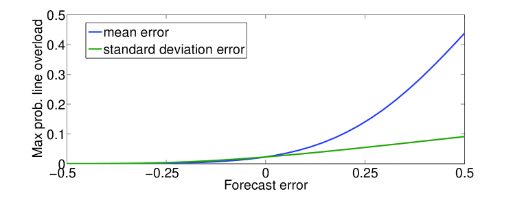
Next we consider the Gaussian case with errors. We solve with nominal values for the mean and standard deviation of wind power. We then consider the rate of violation after scaling all means and standard deviations (separately) . While the solution is sensitive to errors in the mean forecast, the sensitivity is well-behaved. With a desired safety level of for each line, an error in the mean of 25% results in a maximum 15% chance of exceeding the limit. The solution is quite robust to errors in the standard deviation forecast, with a 25% error resulting in less than 6% chance of overload. See Figure 10.
| Distribution | Max. prob. violation |
|---|---|
| Normal | 0.0227 |
| Laplace | 0.0297 |
| logistic | 0.0132 |
| Weibull, | 0.0457 |
| Weibull, | 0.0355 |
| Weibull, | 0.0216 |
| t location-scale, | 0.0165 |
| Cauchy | 0.0276 |
3.8 Scalability
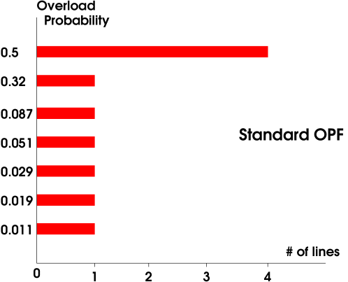
As an additional experiment illustrating scalability of the approach we studied the Polish national grid (obtained from MATPOWER as explained above) under simulated 20 % renewable penetration spread over 18 wind farms, co-located with the 18 largest generators. This co-location should lessen the risk associated with renewable fluctuation (which should be partially “absorbed” by the co-located generators). Figure 11 studies the resulting risk exposure under standard OPF. The chart shows the number of lines that attain several levels of overload probability. The situation in the chart is unacceptable: it would lead to frequent tripping of at least four lines.
In contrast, Figure 12 shows the performance attained by the chance-constrained OPF in the same setting as that of Figure 11. Notice the drastic reduction in overload probabilities – the system is stable. Moreover, this is attained with a minor increase in cost (less than one percent) while the computational time is on the order of 10 seconds.

4 Discussions
This manuscript suggests a new approach to incorporating uncertainty in the standard OPF setting routinely used in the power industry to set generation during a time window, or period (typically 15 min to one hour duration). When uncertainty associated with renewable generation is quantified in terms of the probability distribution of output during the next period, we incorporate it through chance constraints - probabilistic conditions which require that any line of the system will not be overloaded for all but a small fraction of time (at most one minute per hour, for example). Additionally, the modeling accounts for local frequency response of controllable generators to renewable changes. The key technical result of this manuscript is that the resulting optimization problem, CC-OPF, can be stated as a convex, deterministic optimization problem. This result also relies on plausible assumptions regarding the exogenous uncertainty and linearity of the underlying power flow approximations/equations. In fact, our CC-OPF is a convex (conic) optimization problem, which we solve very efficiently, even on realistic large-scale instances, using a sequential linear cutting plane algorithm.
This efficient CC-OPF algorithm becomes an instrument of our (numerical) experiments which were performed on a number of standard (and nonstandard) power grid data sets. Our experimental results are summarized as follows:
-
•
We observe that CC-OPF delivers feasible results where standard OPF, run for the average forecast, would fail in the sense that many lines would be overloaded an unacceptably large portion of time.
-
•
Not only is CC-OPF safer than standard OPF, but it also results in cheaper operation. This is demonstrated by considering the optimal cost of CC-OPF under sufficiently high wind penetration solution (where standard OPF would fail) and the low penetration solution (corresponding to the highest possible penetration where standard OPF would not fail).
-
•
We discover that solutions produced by CC-OPF deviate significantly from what amounts to a the naive adjustment of the standard OPF obtained by correcting dispatch just at those generators which are close to overloaded lines.
-
•
We test the level of wind penetration which can be tolerated without upgrading lines. This experiment illustrates that, at least for the model tested, the 30% of wind penetration with rather strict probabilistic guarantees enforced by our CC-OPF may be feasible; but much lower wind penetration remains feasible under the standard approach.
-
•
We experiment with location of wind farms and discover strong sensitivity of the maximum level of penetration on the choice of location - optimal choice of wind farm location is critical for achieving the ambitious goal of high renewable penetration.
-
•
Analyzing fluctuations of line flows within CC-OPF solution admissible under high wind penetration, we discover that these fluctuations may be significant, in particular resulting in reversal of power flows over some of the lines. This observation suggests that flow reversals and other qualitative changes of power flows, which are extremely rare in the grid of today, will become significantly much more frequent (typical) in the grid of tomorrow.
-
•
We studied an out-of-sample test consisted in applying CC-OPF (modeling exogenous fluctuations as Gaussian) to other distributions. Overall these tests suggest that with a proper calibration of the effective Gaussian distribution our CC-OPF delivers a rather good performance. One finds that the worst CC-OPF performance is observed for the most asymmetric distributions.
-
•
We also presented a computationally sound data-robust version of the CC-OPF where the parameters for the Gaussian distributions are assumed unknown, but lying in a window. This allows for parameter mis-estimation, for model error, and it is suggests a way to deal in a tractable way with non-Gaussian fluctuations.
The nature of the problem discussed in the manuscript – the design of a new paradigm for computationally efficient generation re-dispatch that accounts for wind fluctuations – inevitably required incorporation of a number of assumptions and approximations. In particular, we made simplifying assumptions about static forecasts and general validity of power flow linearization. We have also focused solely on failures associated with line congestion ignoring other possible difficulties, for example those associated with loss of synchronicity and voltage variations. However, we would like to emphasize that all of these assumptions (admittedly natural for a first attack on the problem) also allow generalization within the approach just sketched:
-
•
Accounting for time evolving forecast/loads/etc. Wind forecast, expressed in terms of the mean and standard deviation at the wind farm sites, changes on the scales comparable to duration of the generation re-dispatch interval. Loads may also change at these time scales. When the slowly evolving, but still not constant, wind and load forecasts are available we may keep the quasi-static power flow description and incorporate this slow evolution in time into the chance constrained scheme. These changes will simply result in generalizing the conic formulation (56)-(64) by splitting what used to be a single time interval into sub-intervals and allowing the regular generation to be re-dispatched and parallel coefficients to be adjusted more often. Ramping rate constraints on the controllable generation may naturally be accounted in the temporal optimization scheme as well.
-
•
Accounting for nonlinearity in power flows. Evolution of the base case invalidates the linearization (DC-style) hypothesis. However, if variations around one base case becomes significant one may simply adjust the linearization procedure doing it not once (as in the case considered in the manuscript) but as often as needed. Slow adjustment of the base case may also be included into the dynamical procedure mentioned one item above. Additionally, some interesting new methodologies for handling nonlinearities have recently emerged, see [36].
-
•
Accounting for synchronization bounds. Loss of synchronicity and resulting disintegration of the grid is probably the most acute contingency which can possibly take place in a power system. The prediction of those conditions under which the power grid will lose synchronicity is a difficult nonlinear and dynamic problem. However, as shown recently in [22], one can formulate an accurate linear and static necessary condition for the loss of synchronicity. A chance-constrained version of the linear synchronization conditions can be incorporated seamlessly in our CC-OPF framework.
Finally, we see many opportunities in utilizing the CC-OPF (possibly modified) as an elementary unit or an integral part of even more complex problems, such as combined unit commitment (scheduling large power plants normally days, weeks or even months ahead) [48] with CC-OPF, planning grid expansion [3] while accounting for cost operation under uncertainty, or incorporating CC-OPF in mitigating emergency of possible cascades of outages [16, 40, 44, 43, 8, 9, 24, 5]. In this context, it would be advantageous to speed up our already very efficient CC-OPF even further. See, for example, [10], [7]. A different methodology, relying on distributed algorithms, can be found in [34].
5 Acknowledgments
We are thankful to S. Backhaus and R. Bent for their comments, and to K. Dvijotham for help with BPA data. The work at LANL was carried out under the auspices of the National Nuclear Security Administration of the U.S. Department of Energy at Los Alamos National Laboratory under Contract No. DE-AC52-06NA25396. MC and SH also acknowledge partial support of the DTRA Basic Research grant BRCALL08-Per3-D-2-0022. DB and SH were partially supported by DOE award DE-SC0002676.
References
- [1] S. Baghsorkhi and I. Hiskens, Analysis tools for assessing the impact of wind power on weak grids, SysCon, (2012), pp. 1 –8.
- [2] R. Ben-Tal and A. Nemirovski, Robust solutions of linear programming problems contaminated with uncertain data, Mathematical Programming, 88 (2000), pp. 411–424.
- [3] R. Bent, G. Toole, and A. Berscheid, Transmission network expansion planning with complex power flow models, Power Systems, IEEE Transactions on, 27 (2012), pp. 904 –912.
- [4] A. Bergen and V. Vittal, Power System Analysis, Prentice Hall. Inc, 2000.
- [5] A. Bernstein, D. Hay, M. Uzunoglu, and G. Zussman, Power grid vulnerability to geographically correlated failures - analysis and control implications. http://arxiv.org/abs/1206.1099, 2012.
- [6] D. Bertsimas and M. Sim, Price of robustness, Operations Research, 52 (2004), pp. 35–53.
- [7] D. Bienstock, Potential Function Methods for Approximately Solving Linear Programming Problems, Theory and Practice, Kluwer, 2002.
- [8] D. Bienstock, Adaptive online control of cascading blackouts, Proc. 2011 IEEE Power and Energy Society General Meeting, (2011), pp. 1–8.
- [9] , Optimal control of cascading power grid failures, Proc 2011 CDC-ECC, (2011), pp. 2166 –2173.
- [10] D. Bienstock and G. Iyengar, Faster approximation algorithms for covering and packing problems, SIAM Journal on Computing, 35 (2006), pp. 825–854.
- [11] H. Bludszuweit, J. Dominguez-Navarro, and A. Llombart, Statistical analysis of wind power forecast error, Power Systems, IEEE Transactions on, 23 (2008), pp. 983 –991.
- [12] S. Boyd and L. Vandenberghe, Convex Optimization, Cambridge University Press, 2004.
- [13] BPA-WIND, Wind generation & total load in the bpa balancing authority. http://transmission.bpa.gov/business/operations/wind/, 2012.
- [14] CAISO, Integration of renewable resources: Transmission and operating issues and recommendations for integrating renewable resources on the california iso-controlled grid. http://www.caiso.com/1ca5/1ca5a7a026270.pdf, 2007.
- [15] A. Charnes, W. Cooper, and G. Symonds, Cost horizons and certainty equivalents: an approach to stochastic programming of heating oil, Management Science, 4 (1958), pp. 235–263.
- [16] J. Chen, J. Thorp, and I. Dobson, Cascading dynamics and mitigation assessment in power system disturbances via a hidden failure model, International Journal of Electrical Power; Energy Systems, 27 (2005), pp. 318 – 326.
- [17] M. Chertkov, F. Pan, and M. Stepanov, Predicting failures in power grids: The case of static overloads, IEEE Transactions on Smart Grids, 2 (2010), p. 150.
- [18] M. Chertkov, M. Stepanov, F. Pan, and R. Baldick, Exact and efficient algorithm to discover extreme stochastic events in wind generation over transmission power grids, CDC-ECC, (2011), pp. 2174 –2180.
- [19] CIGRE, Technical brochure on grid integration of wind generation, International Conference on Large High Voltage Electric Systems, (2009).
- [20] CPLEX, ILOG CPLEX Optimizer. http://www-01.ibm.com/software/integration/optimization/cplex-optimizer/, 2012.
- [21] DENA, Energy management planning for the integration of wind energy into the grid in germany, onshore and offshore by 2020, (2005).
- [22] F. Dörfler, M. Chertkov, and F. Bullo, Synchronization in Complex Oscillator Networks and Smart Grids, Proceedings of National Academy of Sciences, 10.1073/pnas.1212134110 (2013).
- [23] EERE, 20% of wind energy by 2030: Increasing wind energy’s contribution to us electricity supply, Department of Energy (DOE), DOE/GO-102008-2567 (2008).
- [24] M. Eppstein and P. Hines, A ”random chemistry” algorithm for identifying collections of multiple contingencies that initiate cascading failure, Power Systems, IEEE Transactions on, 27 (2012), pp. 1698–1705.
- [25] E. Erdogan and G. Iyengar, Ambiguous chance constrained problems and robust optimization, Mathematical Programming, 107 (2007), pp. 37–61.
- [26] U.-C. P. S. O. T. Force, Report on the august 14, 2003 blackout in the united states and canada: Causes and recommendations. https://reports.energy.gov, (2004).
- [27] D. Goldfarb and F. Alizadeh, Second-order cone programming, Mathematical Programming, 95 (2003), pp. 3–51.
- [28] D. Goldfarb and G. Iyengar, Robust portfolio selection problems, Mathematical Programming, 28 (2001), pp. 1–38.
- [29] G. Gonzalez and et al., Experience integrating and operating wind power in the peninsular spanish power system. point of view of the transmission system operator and a wind power producer, CIGRE, (2006).
- [30] M. Grötschel, L. Lovász, and A. Schrijver, Geometric Algorithms and Combinatorial Optimization, Springer-Verlag, 1998.
- [31] GUROBI, Optimizer. http://www.gurobi.com/, 2012.
- [32] B.-M. Hodge and M. Milligan, Wind power forecasting error distributionsover multiple timescales, Detroit Power Engineering Society Meeting, (2011), pp. 1–8.
- [33] M. Huneault, A survey of the optimal power flow literature, Power Systems, IEEE Transactions, (1991).
- [34] M. Kraning, E. Chu, J. Lavaei, and S. Boyd, Message passing for dynamic network energy management. http://www.stanford.edu/~boyd/papers/decen_dyn_opt.html, 2012.
- [35] P. Kundur, Power System Stability and Control, McGraw-Hill, New York, NY, USA, 1994.
- [36] J. Lavaei and S. Low, Zero duality gap in optimal power flow problem, IEEE Transactions on Power Systems, 27 (2012), pp. 92–107.
- [37] Y. Makarov, C. Loutan, J. Ma, and P. de Mello, Operational impacts of wind generation on california power systems, Power Systems, IEEE Transactions on, 24 (2009), pp. 1039 –1050.
- [38] L. Miller and H. Wagner, Chance-constrained programming with joint constraints, Operations Research, 13 (1965), pp. 930–945.
- [39] MOSEK, Optimizer. http://www.mosek.com/, 2012.
- [40] D. Nedic, I. Dobson, D. Kirschen, B. Carreras, and V. E. Lynch, Criticality in a cascading failure blackout model, International Journal of Electrical Power; Energy Systems, 28 (2006), pp. 627 – 633.
- [41] A. Nemirovski and A. Shapiro, Convex approximations of chance constrained programs, SIAM Journal on Optimization, 17 (2006), pp. 969–996.
- [42] U. Ozturk and M. Mazumdar, A solution to the stochastic unit commitment problem using chance constrained programming, Power Systems, IEEE, 19 (2004), pp. 1589–1598.
- [43] R. Pfitzner, K. Turitsyn, and M. Chertkov, Controlled Tripping of Overheated Lines Mitigates Power Outages, arxiv:1104.4558, (2011).
- [44] R. Pfitzner, K. Turitsyn, and M. Chertkov, Statistical classification of cascading failures in power grids, in Power and Energy Society General Meeting, 2011 IEEE, july 2011, pp. 1 –8.
- [45] A. Prékopa, On probabilistic constrained programming, Proc. Princeton Symposium on Math. Programming, (1970), pp. 113–138.
- [46] M. Vrakopoulou, K. Margellos, J. Lygeros, and G. Andersson, A probabilistic framework for security constrained reserve scheduling of networks with wind power generation, in Energy Conference and Exhibition (ENERGYCON), 2012 IEEE International, sept. 2012, pp. 452 –457.
- [47] G. Wang, M. Negrete-Pincetic, A. Kowli, E. Shafieepoorfard, S. Meyn, and U. Shanbhag, Dynamic competitive equilibria in electricity markets, in Control and Optimization Theory for Electric Smart Grids, A. Chakrabortty and M. Illic, eds., Springer, 2011.
- [48] J. Wang, M. Shahidehpour, and Z. Li, Security-constrained unit commitment with volatile wind power generation, Power Systems, IEEE Transactions on, 23 (2008), pp. 1319 –1327.
- [49] M. Wyld, Wind energy bumps into power grid limits, New York Times, (2008/08/27).
- [50] H. Zhang, Chance Constrained Programming for Optimal Power Flow Under Uncertainty, Power Systems, IEEE Transactions on, 26 (2011), pp. 2417–2424.
- [51] S. Zhang, Y. Song, Z. Hu, and L. Yao, Robust optimization method based on scenario analysis for unit commitment considering wind uncertainties, in Power and Energy Society General Meeting, 2011 IEEE, july 2011, pp. 1 –7.
- [52] R. Zimmerman, C. Murillo-Sanchez, and R. Thomas, Matpower: Steady-state operations, planning, and analysis tools for power systems research and education, Power Systems, IEEE Transactions on, 26 (2011), pp. 12 –19.