LOFAR insights into the epoch of reionization from the cross power spectrum of 21 cm emission and galaxies

Abstract

Using a combination of N-body simulations, semi-analytic models and radiative transfer calculations, we have estimated the theoretical cross power spectrum between galaxies and the 21 cm emission from neutral hydrogen during the epoch of reionization. In accordance with previous studies, we find that the 21 cm emission is initially correlated with halos on large scales ($\;\buildrel>\over{\sim}\;$30 Mpc), anti-correlated on intermediate ($\sim 5$ Mpc), and uncorrelated on small ($\;\buildrel<\over{\sim}\;$3 Mpc) scales. This picture quickly changes as reionization proceeds and the two fields become anti-correlated on large scales. The normalization of the cross power spectrum can be used to set constraints on the average neutral fraction in the intergalactic medium and its shape can be a powerful tool to study the topology of reionization. When we apply a drop-out technique to select galaxies and add to the 21 cm signal the noise expected from the LOFAR telescope, we find that while the normalization of the cross power spectrum remains a useful tool for probing reionization, its shape becomes too noisy to be informative. On the other hand, for a Ly$\alpha$ Emitter (LAE) survey both the normalization and the shape of the cross power spectrum are suitable probes of reionization. A closer look at a specific planned LAE observing program using Subaru Hyper-Suprime Cam reveals concerns about the strength of the 21 cm signal at the planned redshifts. If the ionized fraction at $z\sim 7$ is lower that the one estimated here, then using the cross power spectrum may be a useful exercise given that at higher redshifts and neutral fractions it is able to distinguish between two toy models with different topologies.

1 Introduction

The epoch of reionization (EoR) is considered one of the great observational frontiers in astronomy today. It forms the crucial bridge between the epoch of recombination and the galaxies we currently observe. Since it was the era of first substantial galaxy formation, it provides the context in which to understand the local universe. The reionization process itself likely had a direct impact on further galaxy formation and growth, primarily due to the dramatic change in temperature of the Intergalactic Medium (IGM) caused by the photo-ionization.

The investigation of the EoR takes place on both theoretical and observational fronts. From the theoretical perspective, analytic models of reionization have been employed since Arons & Wingert (1972) and Hogan & Rees (1979) and improved versions are still being developed (e.g. Furlanetto & Loeb, 2005; Choudhury & Ferrara, 2006; Bolton & Haehnelt, 2007). While these models display a high degree of sophistication, the non-linear nature of the feedback of reionization upon further galaxy formation is not typically captured. Approaches based on (semi-)numerical methods can incorporate such and other complexities, as for example the three-dimensional effects of shadowing and the overlap of ionized regions. This allowed them to treat more of the physics properly, although this comes of course at the cost of computing time.

All these theoretical investigations have considerably advanced our understanding of the progress of reionization, in particular the effect of inhomogeneities in the radiation field, the relative importance of minihalos, quasars, and regular galaxies, and the topology of reionization (e.g. Ciardi et al., 2000; Gnedin, 2000; Razoumov et al., 2002; Ciardi et al., 2003; Sokasian et al., 2003; Iliev et al., 2006; Kohler et al., 2007; Zahn et al., 2007; Thomas & Zaroubi, 2011; Ciardi et al., 2011).

However, numerical simulations also have their limitations. To make such calculations feasible for a representative sample of the Universe, several assumptions/simplifications must be made. These simplifications are a result of both the uncertainty in the physics (e.g., star formation efficiency, properties of the ionizing sources, escape fraction) and the finite computing resources which entail a certain finite resolution for the simulation. Hence, to span the parameter space of interest, methods typically resort to various Monte Carlo and post-processing techniques that do not capture feedback effects self-consistently (e.g. Ciardi et al., 2000; Thomas & Zaroubi, 2011).

On the observational front, probing the EoR directly has been difficult and to date our main constraints on the time interval during which reionization occurred are the Thomson scattering optical depth at high redshift (Komatsu et al., 2011) and the absence of Gunn-Peterson troughs at the lower redshift end (e.g. Fan et al. 2006; Becker et al. 2007, but see also Schroeder et al. 2012 for the detection of Gunn-Peterson damping wings).

In pursuit of a direct detection of the EoR, a number of instruments in various phases of development will be used to attempt to detect neutral hydrogen via its 21 cm hyperfine transition. PAPER, LOFAR, 21CMA, GMRT, MWA, and eventually SKA all hope to detect the 21 cm signal from the EoR. It is not only the detection of the trend in the decline (from higher to lower redshift) of the global neutral hydrogen content that will be informative. Also of interest will be the spatial distribution/fluctuations of the 21 cm signal at a given redshift.

In these early attempts, detecting the 21 cm signal from the EoR will be extremely challenging. To alleviate some of the problems, several cross-correlation analyses with observations in other wavelength regimes have been proposed. Under the assumption that the noise and uncertainties will be mitigated by using two observations of such different character, we can hope to put constraints on the nature of reionization and hence gain further insights into the processes active during the EoR. In recent years several authors have undertaken theoretical studies of the cross-correlation analysis of 21 cm measurements with other observations. Correlations with the cosmic microwave background (CMB) (Salvaterra et al., 2005; Adshead & Furlanetto, 2008; Berndsen et al., 2010; Jelić et al., 2010), galaxy surveys (Lidz et al., 2009) and CO-emission surveys (Lidz et al., 2011) have already been proposed. This type of analysis is particularly timely also in view of the exciting progress made in the observation of high-redshift galaxies (e.g. Ouchi et al. 2010; Bouwens et al. 2012 and references therein), which is promising to provide a large, statistically significant sample of such objects in the near future.

In this paper, we make predictions for the observation of the cross-correlation between the 21 cm and galaxy fields along the lines of Lidz et al. (2009), but tailored towards the LOFAR-EoR experiment and the future high-redshift Subaru galaxy surveys. Using a dark matter simulation and an efficient radiative transfer code, we begin by cross-correlating the distribution of dark matter halos with the distribution of the 21 cm signal. We continue by using a well-studied semi-analytic model for galaxy formation and evolution to populate the halos with galaxies, thereby incorporating realistic detection and identification limits for the galaxies. We also add the expected noise characteristics from LOFAR to the 21 cm signal to determine the use of galaxy-21cm cross-correlation for detecting and characterizing reionization.

This paper is organized as follows: §2 specifies the dark matter simulation, radiative transfer code and the method used to construct the cross power spectrum. In §3 we calculate the cross power spectrum without imposing any observational limitations, in order to find the theoretically predicted best possible scenario for the detection. In §4 we see how introducing more realistic specifications for both the 21 cm and the galaxy survey modifies the theoretical result. Finally, in §5 we discuss these results and the viability of performing such a cross-correlation in practice.

2 Method

Following Lidz et al. (2009), we define the cross power spectrum between the 21 cm emission and the galaxies as:

$$\begin{array}[]{lll}\Delta^{2}_{\rm 21,gal}(k)&=&\tilde{\Delta}^{2}_{\rm 21,gal}(k)/\delta T_{b0}\\ &=&\langle x_{\textsc{hi}}\rangle\left[\Delta^{2}_{x,{\rm gal}}(k)+\Delta^{2}_{\rho,{\rm gal}}(k)\right.\\ &&\left.+\Delta^{2}_{x\rho,{\rm gal}}(k)\right].\end{array}$$ (1)

The 21cm–galaxy cross power spectrum is thus made up from the sum of three other cross power spectra, the neutral fraction–galaxy cross power spectrum, $\Delta^{2}_{x,{\rm gal}}$, the density-galaxy cross power spectrum, $\Delta^{2}_{\rho,{\rm gal}}$, and the neutral density–galaxy cross power spectrum, $\Delta^{2}_{x\rho,{\rm gal}}$. In Equation 1 we defined $\Delta^{2}_{\rm 21,gal}(k)$ such that the 21 cm brightness temperature relative to the CMB for neutral gas at the mean density of the universe $\delta T_{b0}$ is scaled out (normalized cross power spectrum), since the 21 cm field can be given by $\delta_{\rm 21}(r)=\delta T_{b0}\langle x_{\textsc{hi}}\rangle(1+\delta_{x}(r))(1+\delta_{\rho}(r))$, where $\langle x_{\textsc{hi}}\rangle$ is the mean volume averaged neutral fraction and $\delta_{i}(r)$ represents the spatial field $i$ with respect to its mean, e.g. $\delta_{i}(r)=(i(r)-\langle i\rangle)/\langle i\rangle$. For the neutral hydrogen field, $i$ refers to $x_{\rm HI}(r)$, the fraction of hydrogen that is neutral at position $r$, while for the galaxy field, $i$ refers to $n_{\rm gal}(r)$, the number density of galaxies at $r$. Finally, we work with the dimensionless cross power spectrum, i.e. $\Delta^{2}_{a,b}(k)=k^{3}P_{a,b}(k)/(2\pi^{2})$ for the 3D power spectrum and $\Delta^{2}_{a,b}(k)=2k^{2}P_{a,b}(k)$ for the 2D power spectrum, where $P_{a,b}$ is the dimensional cross power spectrum between fields $a$ and $b$. We refer the reader to Lidz et al. (2009) for a more detailed discussion of the three terms in Equation 1.

In order to construct the cross power spectrum, we therefore require three fields, the density field, the neutral hydrogen field, and the galaxy field.

For this work we make use of the well-studied Millennium Simulation (Springel et al., 2005). It is a dark matter simulation featuring $2160^{3}$ particles in a $500h^{-1}\,{\rm Mpc}$ comoving box run from $z=127$ down to $z=0$. It was run in a $\Lambda$CDM cosmology with $(\Omega_{m},\Omega_{\Lambda},\Omega_{b}h^{2},h,\sigma_{8},n)=(0.25,0.75,0.024,0.73,0.9,1.)$, which implies a particle mass of $1.2\times 10^{9}{{\rm M}_{\odot}}h^{-1}$. We have scaled the cosmology to the more recent WMAP7 measurements found in (an early version of) Komatsu et al. (2011) – $(\Omega_{m},\Omega_{\Lambda},\Omega_{b}h^{2},h,\sigma_{8},n)=(0.272,0.728,0.02246,0.702,0.807,0.961)$ – in accordance with the method described in Angulo & White (2010), scaling the output redshift, distance coordinates and particle masses. All quantities are transferred to a $256^{3}$ grid, using a cloud-in-cell scheme for the density and galaxy fields.

Halos with masses greater than $10^{10}{{\rm M}_{\odot}}$ (corresponding to a limit of 20 particles) are selected as sources; not only do we reduce resolution effects with such a cut, Lidz et al. (2009) used a similar limit. The spectrum assumed is that of a young, metal-poor stellar population whose spectral energy distribution (SED) was determined using starburst99 (Leitherer et al., 1999) and is scaled according to the mass of the halo. The escape fraction of ionizing photons from each halo is taken to be 10%. The density and source field from the simulation, together with the SED, are given as input to the bears code (Thomas et al., 2009) to calculate the neutral hydrogen field. bears is a radiative transfer code that, given the luminosity of a source and its spectrum, calculates a spherically averaged density profile around the source and embeds a spherically symmetric ionization bubble. These bubbles are drawn from a catalogue of 1D radiative transfer results of various types of spectra, luminosities, redshifts and density profiles. The code deals with overlapping HII regions by increasing the sizes of the bubbles involved in the overlap in such a way that the volume matches that of the overlap regions, hence conserving photons. The reionization histories calculated using bears give a value of Thompson scattering optical depth which is $\sim 0.09$ and within the 1-$\sigma$ error bar of the WMAP3 estimate. For more details of the 1D radiative transfer code, the implementation of bears and its extensions, see Thomas & Zaroubi (2008), Thomas et al. (2009) and Thomas & Zaroubi (2011).

It has to be noted that the resolution of the simulations does not allow us to resolve the population of galaxies that are thought to be responsible for the production of the majority of the ionizing photons during reionization, which reside in halos that cool via atomic and molecular transitions roughly in the range of $10^{6}-10^{9}\mathrm{M_{\odot}}$ (e.g. Muñoz & Loeb, 2011; Raičević et al., 2011). The clustering bias should, however, not be strong enough to affect our results too much.

The output of the bears code is the neutral fraction throughout our simulation volume at different redshifts. To calculate the 21 cm-galaxy cross power spectrum we need to calculate the 21 cm differential brightness temperature, which is defined as follows (e.g. Thomas et al., 2009):

$$\begin{array}[]{ll}\delta T_{b}(r)=&19{\rm mK}(1+\delta(r))\left(\displaystyle\frac{x_{\rm\textsc{hi}}(r)}{h}\right)\left(1-\displaystyle\frac{T_{\rm CMB}}{T_{s}(r)}\right)\\ &\times\left[\displaystyle\frac{H(z)/(1+z)}{{\rm d}v_{||}/{\rm d}r_{||}}\right]\left(\displaystyle\frac{\Omega_{b}h^{2}}{0.02246}\right)\\ &\times\left[\left(\displaystyle\frac{1+z}{10}\right)\left(\displaystyle\frac{0.272}{\Omega_{m}}\right)\right]^{1/2},\end{array}$$ (2)

where $\delta(r)$ is the matter overdensity at position $r$, $T_{\rm CMB}$ is the CMB temperature, $T_{s}(r)$ is the spin temperature, and the other symbols have their usual meanings. We make the approximations that $T_{s}(r)\gg T_{\rm CMB}$ everywhere and that the peculiar velocities do not contribute, such that the fourth and fifth terms are unity (see Mao et al., 2011, for a discussion on the contribution of peculiar velocities to the 21 cm power spectrum).

When calculating cross power spectra and correlation functions (see the following section) we bin the quantities such that $\Delta$log$k=0.02$; for low $k$, we merge bins such that $\Delta k>0.05$ to ensure that our points are not correlated by the window function. For all figures in this paper, we plot quantities against co-moving $k$.

In Fig. 1 we show the spherically averaged 3D 21 cm power spectrum for the redshifts we will concentrate on throughout this work. The power spectrum shows the usual shape, with the normalization decreasing as the age of the universe (and mean ionized fraction) increases, the large scale power being the last to decrease. Initially there is much power on small scales due to the clustered density profile. At later times, however, the small-scale power diminishes as the large-scale power remains.

3 The theoretical 21 cm – halo cross power spectrum

Before concerning ourselves with what will be detected by upcoming observations, it is useful to understand the intrinsic behaviour of the 21 cm – galaxy cross power spectrum. To study this, we use the dark matter halos that we described in the previous section to represent the galaxy field. Here we make no attempt to discern what will be detectable or identified as a galaxy in the specified redshift range.

Fig. 2 shows the spherically averaged 3D 21 cm – halo cross power spectrum for $z=8.32$, when the mean fraction of neutral hydrogen is $\langle x_{\rm\textsc{hi}}\rangle=0.53$. Here we have broken it down into the three components listed in Equation 1, where the black solid curve is the final result. It is worth remarking that, while $\Delta^{2}(k)_{\rho,{\rm gal}}$ is always positive, $\Delta^{2}(k)_{x\rho,{\rm gal}}$ is always negative and $\Delta^{2}(k)_{x,{\rm gal}}$ is negative for $k$ where there are no oscillations. This implies an anti-correlation is measured for the last two fields.

Taking each term in turn, the density-galaxy cross power spectrum, $\Delta^{2}(k)_{\rho,{\rm gal}}$, is the most straightforward component to interpret. On small scales, these two fields correlate very strongly, reminding us that halo formation is biased to high density regions. The power decreases, however, towards large scales at which halos are much less aware of the density. The increase of power is roughly two orders of magnitude over two orders in magnitude in scale.

The reionization process in our simulation proceeds in an ‘inside-out’ fashion, that is high density regions are typically ionized earlier than low density regions. At the redshift we are considering here large-scale underdense regions are still mostly neutral and free of galaxies, whereas the overdense regions surrounding the galaxies have all become ionized. This leads to an anti-correlation between the galaxy and neutral fraction fields, the strength of which increases with decreasing scale, as illustrated by the behaviour of the $\Delta^{2}(k)_{x,{\rm gal}}$ term in Fig. 2. Depending on the details of the model and the redshift, a turn around manifests with a positive correlation on scales at which the galaxies correlate with the density field. On sub-bubble scales the correlation is expected to die off because the interior of an HII region is ionized independently from the local galaxy field. The typical size of the ionized bubbles is then imprinted on the cross power spectrum at the smallest scales with an oscillatory behaviour. This behaviour is less pronounced in Lidz et al. (2009) because they can resolve smaller scales and lower mass halos. As a result their reionization topology is less dominated by large bubbles. Since bubbles are a generic feature of reionization, we do not expect that the oscillations will disappear altogether in the high resolution limit, but would tend towards the noise-like shape found in Lidz et al. (2009).

Finally, the $\Delta^{2}(k)_{x\rho,{\rm gal}}$ term, which is not very significant on large scales, serves to cancel the galaxy – density cross power spectrum almost entirely at small scales (recall that they have different signs). This effect is particularly strong for k-modes for which the size of the ionization bubble is imprinted.

All three terms added give the measurable term, the 21 cm – galaxy cross power spectrum. Its shape is mainly determined by the $\Delta^{2}(k)_{\rho,{\rm gal}}$ and $\Delta^{2}(k)_{x,{\rm gal}}$ terms on large scales, and almost completely by the latter at small scales. This confirms the findings of Lidz et al. (2009) and we refer the reader to their work for further discussion.

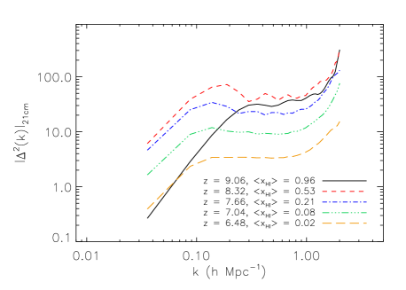
Figure 1: The spherically averaged 3D 21 cm auto power spectrum for various redshifts/mean neutral fractions in our simulations. Power (particularly at small scales) decreases with decreasing neutral fraction.

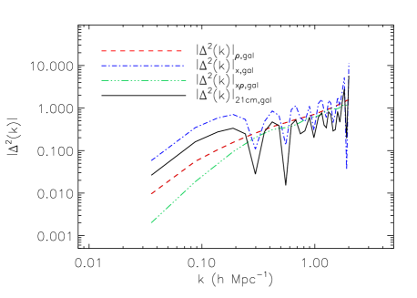
Figure 2: The spherically averaged 3D 21 cm – halo cross power spectrum for $z=8.32$, corresponding to $\langle x_{\rm\textsc{hi}}\rangle=0.53$. Also shown are the components of the 21 cm – halo cross power spectrum.

To better understand the behaviour of the cross power spectrum, we now study two toy models. For the first model we begin with a neutral universe and place ionized spheres with radius approximately $8h^{-1}\,{\rm Mpc}$ around halos with mass greater than $10^{10}{{\rm M}_{\odot}}$ (this value gives an ionized fraction of roughly $50\%$). The second model is the dual of the first: the background universe is taken to be ionized and the bubbles contain neutral hydrogen. For both we use the same density field and halo distribution as above, namely the one from redshift $z=8.32$, where also the bears simulation had $\langle x_{\rm\textsc{hi}}\rangle\approx 0.5$.

We show the cross power spectrum and the cross-correlation coefficient for these models, as well as the prediction from bears (black solid line in Fig. 2) in Fig. 3. The first thing we notice is that all three curves look remarkably similar. In the toy models the oscillations begin at larger k since the characteristic size of neutral regions is larger compared to the radiative transfer approach. The bottom panel shows the cross-correlation coefficient, defined as $r(k)=P_{21,{\rm gal}}(k)/[P_{21}(k)P_{\rm gal}(k)]^{1/2}$. Here we confirm that for the neutral bubble model the 21 cm emission is strongly correlated with the halo positions on large scales. At smaller scales the halo density is uncorrelated with the 21 cm emission since an $8h^{-1}\,{\rm Mpc}$ bubble can contain many or one halo.

Naturally, the size of our toy bubbles is arbitrary and has been chosen so that the average neutral fraction is $\approx 0.5$ for all models. If we were to use larger bubbles (they would need to be less ionized to maintain our restriction of a global ionized fraction of roughly $50\%$) we would expect the oscillations to occur at slightly lower $k$, while we would expect the opposite for smaller bubbles. This implies that the characteristic size of the bubbles in the bears simulation is slightly larger than $8h^{-1}\,{\rm Mpc}$, likely owing to the dominance of high mass sources.

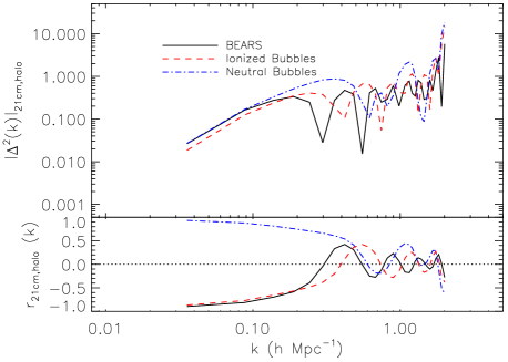
Figure 3: The spherically averaged 3D 21 cm – halo cross power spectrum (upper panel) and cross-correlation coefficient (lower panel) for two toy models at $z=8.32$, $\langle x_{\rm\textsc{hi}}\rangle\approx 0.5$. The black solid line shows the result using bears, while the red dashed line shows a toy model in which $8h^{-1}\,{\rm Mpc}$ ionized bubbles are placed around halos, and the blue dot-dashed line shows a scenario where $8h^{-1}\,{\rm Mpc}$ neutral bubbles are placed around halos in a fully ionized universe. In these extreme cases the general behaviour in the cross power spectrum is similar.

Just as the normalization of the 21 cm auto power spectrum decreases with decreasing neutral fraction, so does the 21 cm – halo cross power spectrum. This is seen in Fig. 4, where we plot the cross power spectrum from the bears results for our selected redshifts. Note that the scale on which the oscillations occur increases with decreasing redshift as the bubbles grow. The power spectrum also becomes flatter as the correlations on small scales diminish.

The lower panel of Fig. 4 shows the correlation coefficient for the same set of redshifts. Here we see that at early times ($z\sim 9$), the signals are strongly anti-correlated on intermediate scales ($k\sim 0.3-0.4$). This is because the bubbles are still small. As the ionized regions become larger, the signals become anti-correlated only on large scales.

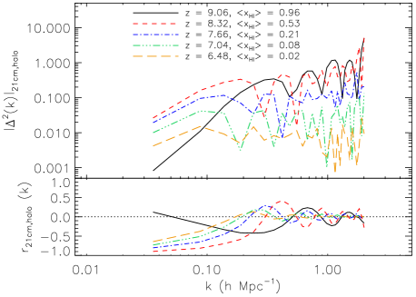
Figure 4: The spherically averaged 3D 21 cm – halo cross power spectrum (upper panel) and correlation coefficient (lower panel) for various redshifts/mean neutral fractions in our simulations. The anti-correlation is very strong on medium scales, but diminishes as the universe becomes more neutral.

All of this conforms to the results found in Lidz et al. (2009). We now turn to a more careful prediction of the observed signal.

4 Predictions for the observed 21 cm – galaxy cross power spectrum

The spherically averaged 21 cm – galaxy (halo) cross power spectrum will not be directly measured by observations. In practice, the cross power spectrum will be circularly averaged after the galaxy field has been projected onto two dimensions, the galaxy sample will be constrained by some selection criteria, and there will be substantial instrumental effects for both the 21 cm signal and the galaxy sample.

We make use of the De Lucia et al. (2006) semi-analytic models (SAM) to generate the necessary galaxy data. This is a well studied model that roughly reproduces many $z=0$ observations. The semi-analytic galaxy catalogue contains both rest-frame and observer-frame magnitudes of many bands. To account for the change in cosmology, we scale the magnitudes of the galaxies with the same mass factor mentioned in section 2, and convert the wavelength of the bands to account for the shift in redshift. In Table 1 we compare the original bands to the converted bands. We caution that this model is designed to fit local universe data, and that its predictions for the high-redshift universe may not be correct. On the other hand, the SAM acts as a ‘best guess’ since fully analytic calculations would neglect the interplay between galaxies, while hydrodynamic simulations would likely underestimate the star formation rate at these redshifts (e.g. Schaye et al., 2010).

To perform our predictions, we consider a very large observational survey. A particularly ambitious program would cover 3 x 3 square degrees and overlap with previously well-studied fields (e.g. the Subaru Deep Field – Kashikawa et al. 2004 and GOODS – Giavalisco et al. 2004). We consider surveys for two types of sources, high-redshift Lyman break galaxies (LBGs) and Lyman alpha emitters (LAEs). The former uses broad band photometry combined with a drop-out technique to detect the rest-frame 912 Å break. Such surveys typically use a strong colour cut to distinguish LBGs from other objects (e.g. Bouwens et al., 2008). They have the advantage that existing filters can be used and combined with already well-studied fields. One large disadvantage is that precise redshifts cannot be determined without spectroscopic follow-up.

LAEs, on the other hand, are objects that emit very strongly in the 1216 Å Ly$\alpha$ line. They are typically found using narrow-band surveys (e.g. Ouchi et al., 2010). Since a narrow filter is used, the redshifts of the objects are rather tightly constrained. The precise nature of LAEs is, however, currently unknown.

4.1 Predictions for drop-out surveys

We search for LBGs at all redshifts of interest, using the detection limits of the survey presented in Ouchi et al. (2009). Their selection criteria were that an object must not be detected in their 4 blue continuum bands (${U,B,V,R}>{27.4,28.0,26.7,27.0}$) and at the same time have a $z^{\prime}-y$ colour greater than 1.5. We relax this colour criterion to 1, and instead of looking at the Ly$\alpha$ trough as they did, we consider the Lyman break since the positioning of our observing bands is determined by the SAM and we can therefore not centre so precisely on the Ly$\alpha$ trough. Table 1 shows how the SAM output bands are affected by the redshift scaling and how they relate to the bands used for the Ouchi et al. (2009) selection.

Table 2 gives the detection efficiency of our galaxies for each redshift of interest. Galaxies are most efficiently detected at redshift 7.66 ($\langle x_{\rm\textsc{hi}}\rangle=0.21$), likely due to a combination of two factors. First, a greater fraction of galaxies are detectable than at higher redshift since the instruments can detect galaxies with a lower absolute magnitude, and second, there is a higher fraction of bright, star-forming galaxies than at lower redshift. The total number of detected galaxies decreases at $z=7.04$ ($\langle x_{\rm\textsc{hi}}\rangle=0.081$) because for this redshift the Lyman break falls in the middle of one of the bands, so the colour difference cannot be efficiently detected.

Table 1: Central wavelength of bands in the observer frame of reference from the original SAM catalogue (left column), the catalogue converted to account for a different cosmology (central) and observed bands (right). See text for details.

Original SAM band	Converted band1	Corresponding
		observed band
u (3500 Å)	2947 Å	U (3600 Å)
g (4800 Å)	4042 Å	B (4400 Å)
r (6250 Å)	5263 Å	V (5500 Å)
i (7700 Å)	6485 Å	R (6400 Å)
z (9100 Å)	7662 Å	z’ (9100 Å)
J (12600 Å)	10610 Å	y (9860 Å)

¹ The actual value varies slightly ($\pm$10 Å) with redshift so we give approximate values here.

Table 2: Number of galaxies in the simulation box (second column), those selected as observable LBGs (third column), and those selected as LAEs (final column). See text for details.

Redshift	Total number	Selected	Selected
	of galaxies in the SAM	LBGs	LAEs
9.06	72791	130	153
8.32	189904	351	581
7.66	420591	768	1940
7.04	820361	421	5517
6.48	1436450	1661	13109

In a drop-out survey without any spectroscopic follow-up, there will be no radial distance information and all of the objects will be projected onto the same plane. The filter width used for these telescopes is less than the width of our simulation box, so we choose to project only a random slab of the box with a thickness that roughly corresponds to 1000 Å, which is the typical full-width at half maximum of the response function that is used in photometric surveys. The SAM outputs a galaxy catalogue gridded according to a count-in-cell scheme. For each line of sight through the slab, we calculate the mean number density weighted by a Gaussian function ($\sigma=0.25l$, where $l$ is the thickness of the slab) to approximate the filter response function since each filter has a different response function anyway . The 21-cm signal is an equally weighted average across the entire slab.

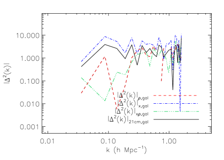
Figure 5: The circularly averaged 2D 21 cm – galaxy cross power spectrum for $z=8.32$, $\langle x_{\rm\textsc{hi}}\rangle=0.53$ for a dropout survey. Also shown are the components of the 21 cm – galaxy cross power spectrum. The general shape and normalization of the power is recovered, but a number of features are lost.

In Fig. 5 we plot the projected, circularly averaged, 21 cm – galaxy cross power spectrum predicted from our simulations for $z=8.32$ ($\langle x_{\rm\textsc{hi}}\rangle=0.53$). Note that since the galaxies are projected, $k$ describes wavenumbers along angular distances. We have again broken it into the individual components from Equation 1. Note that for this figure we have not yet included the noise in the 21 cm signal. We notice immediately that the power spectra are much noisier, and the oscillations observed in Fig. 2 are absent. On the other hand, some general trends are retained, such as the increase of power with decreasing scale. Also as before, the $\Delta^{2}_{x,{\rm gal}}(k)$ term defines the shape for the 21 cm – galaxy cross power spectrum.

Next we add noise appropriate to a 600 h observation with the LOFAR core to the redshifted 21 cm signal. The actual LOFAR station positions are used to generate $uv$ tracks for a 4 h observation at the zenith. From this we define a sampling function $S(u,v)$ which describes how densely the interferometer baselines sample Fourier space over the course of an observation, such that $1/\sqrt{S}$ is proportional to the noise on the measurement of the Fourier transform of the sky in each $uv$ cell. We generate uncorrelated, complex Gaussian noise in each cell, but enforce the condition $n(u,v)^{*}=n(-u,-v)$ where $n(u,v)$ is the noise in the cell with coordinates $(u,v)$. This ensures that when we perform a two-dimensional Fourier transform of this noise realization to obtain a noise image, the image is real. The noise image is normalized to ensure it has a temperature rms

$$\sigma_{\mathrm{noise}}=\frac{\lambda^{2}T_{\mathrm{sys}}}{A_{\mathrm{eff}}\Omega_{\mathrm{beam}}\sqrt{2n_{\mathrm{s}}(n_{\mathrm{s}}-1)t_{int}\Delta\nu}},$$ (3)

where $\lambda$ is the observed wavelength, $T_{\mathrm{sys}}$ is the observed temperature, $A_{\mathrm{eff}}$ is the effective area of a LOFAR station, $n_{\mathrm{s}}$ is the number of stations, $t_{int}$ is the integration time, $\Delta\nu$ is the bandwidth and $\Omega_{\mathrm{beam}}$ is the area of the synthesized beam. We take $T_{\mathrm{sys}}=140+60(\nu/300\ \mathrm{MHz})^{-2.55}\ \mathrm{K}$ and use values for the effective area tabulated on the ASTRON LOFAR webpage.

Since some upcoming surveys are expected to cover very large fields (upwards of three by three square degrees, corresponding to $\sim 60$ proper Mpc at $z=6.48$), we take 4 random slabs (for a square configuration these correspond to $\sim 77$ proper Mpc) through the box and average them to make our predictions less susceptible to sample variance.

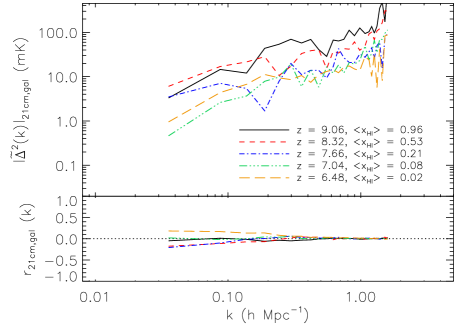
Figure 6: The circularly averaged, unnormalized 2D 21 cm – galaxy cross power spectrum (upper panel) and correlation coefficient (lower panel) for various redshifts/mean neutral fractions in our simulations in the dropout survey case. Although noisy, some of the general trends of the spherically averaged 3D power spectrum are recovered.

In Fig. 6 we present the result for our output redshifts of interest. Please note that this figure shows the true measured (unnormalized) cross power spectrum between the galaxy field and the 21 cm emission, $\tilde{\Delta}^{2}_{\rm 21,gal}(k)$, as defined in Equation 1, and not the normalized one as in the previous figures. Very few of the trends seen in Fig. 4 are recovered. The behaviour of increasing power with decreasing scale is maintained, but the oscillations have all but disappeared. The normalization of the cross power spectrum increases on all scales with decreasing redshift, but the effect is small, such that it would be difficult to distinguish between reionization states using the cross power spectrum alone. The cross correlation coefficients (shown in the bottom panel) are quite noisy and provide little information.

This indicates that using simple detection and selection techniques will make it extremely difficult to glean information from the 21 cm – galaxy cross power spectrum. In our case, we simply do not detect enough galaxies at the highest redshifts, too much information is lost in the projection of the galaxy field, and the observing noise is too large for a significant statement to be made.

Fig. 7 shows the impact that the LOFAR noise has at $z=6.48$ (red lines) and at $z=8.32$ (black lines). Here we see that in the absence of noise (dashed lines), the two redshifts appear to be quite distinct. When noise is introduced (solid lines), the curves appear more similar. While at large scales adding the noise always decreases the power spectrum, at small scales its effect depends on redshift. In fact, unlike for the auto power spectrum where adding the noise always adds to the power, in the cross power spectrum adding the noise moves the spectrum towards what it would be in the case where the galaxy field is crossed with a pure noise field. This means that at $z=8.23$ the cross power spectrum between the pure noise and galaxy fields is lower than the one of the 21 cm and galaxy fields, whereas at $z=6.48$ the 21 cm signal is reduced by a much larger factor than the noise is, resulting in opposite behaviour. This is seen only at small scales because these are the ones where the drop in signal is more significant (see Fig. 4). In other words, after the noise is introduced, the $\Delta^{2}(k)_{x\rho,{\rm gal}}$ and $\Delta^{2}(k)_{x,{\rm gal}}$ terms have diminished influence, while the dominant term becomes $\Delta^{2}(k)_{\rho,{\rm gal}}$.

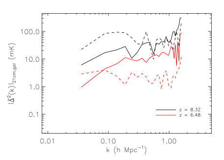
Figure 7: The circularly averaged, unnormalized 2D 21 cm – galaxy cross power spectrum calculated with (solid lines) and without (dashed lines) LOFAR noise in the dropout survey case. The noise inherent in the LOFAR instrument causes the two measurements to become similar.

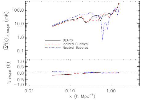
Figure 8: The circularly averaged, unnormalized 2D 21 cm – galaxy cross power spectrum (upper panel) and correlation coefficient (lower panel) for two toy models at $z=8.32$, $\langle x_{\rm\textsc{hi}}\rangle=0.53$ in the dropout survey case. The correlation coefficient is able to distinguish between the two scenarios.

Finally, we revisit our toy models to determine if the observed cross power spectrum can tell us anything about the topology of reionization. We have used the same toy models mentioned in the previous section and have applied the same procedure described in this section. In Fig. 8 we see that these two very different reionization scenarios result in a similar cross power spectrum. There is certainly more power on medium to large scales in the neutral bubble case, indicating that the cross power spectrum could help identify different scenarios. One area in which these two scenarios were distinct in section 3 was the cross-correlation coefficient. In the lower panel of Fig. 3 they were markedly different on large scales. In Fig. 8, the difference is best noticed on medium scales.

4.2 Predictions for LAE surveys

Ouchi et al. (2010) report how they refined their dropout technique using a narrow band filter to identify LAEs. They then obtained follow-up spectra to establish the redshifts of their galaxies. While only a narrow band in redshift is probed, the three dimensional positions of the objects can be established much more precisely.

We can therefore follow a similar procedure as we did in the previous section, with a few slight modifications. The width of the narrow-band filter used by Ouchi et al. (2010) is 132 Å, which roughly corresponds to the a slab about half the thickness considered in the previous section. Since their filter is focused on a very narrow band that we do not have access to in the semi-analytic model, we cannot select based on the same colour criterion they used. Therefore, we use the star-formation rate to intrinsic Ly$\alpha$ luminosity conversion reported in Dayal et al. (2008):

$$L_{\alpha}^{int}=2.80\times 10^{42}{\rm erg~{}s^{-1}}\displaystyle\frac{\rm SFR}{{{\rm M}_{\odot}}{\rm yr^{-1}}}.$$ (4)

This will be attenuated and modified by a number of factors: the escape fraction of ionizing photons, the fraction of Ly$\alpha$ photons that are destroyed by dust, gas inflows and outflows, and any intergalactic absorption and scattering (see e.g. Dijkstra et al. 2007; Kobayashi et al. 2007; Dijkstra & Wyithe 2010; Jeeson-Daniel et al. 2012). The latter is expected to be particularly relevant at these redshifts, when a substantial neutral fraction is expected, but it is beyond the scope of this paper to investigate this issue in more details. We defer further analysis to the future. In order to select a similar number of galaxies as Ouchi et al. (2010) (see below), we assume the transmitted Ly$\alpha$ luminosity to be a factor of 150 less than the intrinsic.

Ouchi et al. (2010) report that they are sensitive to a Ly$\alpha$ luminosity of $2.5\times 10^{42}{\rm ergs^{-1}}$ at $z=6.56$. We have converted this using Equation 4 to act as a star-formation rate cut on our galaxies at each of our redshifts of interest. We use their detection limits to ensure that there is no continuum emission bluewards of the Ly$\alpha$ break.

In Table 2 we give the detection efficiency for the entire box. Since we only take a slab, the actual number of galaxies will be the number in the right-hand column adjusted for the slab thickness. We note that Ouchi et al. (2010) detected 207 LAEs at $z\approx 6.6$ in a plane of similar size to ours; given that we use a slab thickness of 11 (out of 256) at this redshift, we only slightly overestimate the number of detectable LAEs (albeit at a lower redshift).

Fig. 9 is the analogue of Fig. 5. Most of the features found in the dropout cross power spectrum persist for the LAEs. Interestingly, the $\Delta^{2}(k)_{x,~{}{\rm gal}}$ term dominates even more here. Note that for this figure we have not included the noise in the 21 cm signal.

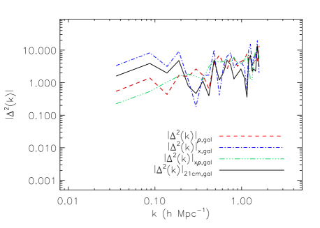
Figure 9: The circularly averaged 2D 21 cm – galaxy cross power spectrum considering a LAE survey for $z=8.32$, $\langle x_{\rm\textsc{hi}}\rangle=0.53$. Also shown are the components of the 21 cm – galaxy cross power spectrum. The general trend of Fig. 5 is maintained.

In Fig. 10 we show the 21 cm – LAE cross power spectrum and correlation coefficient for a number of redshifts. Here we have again averaged the calculation over 4 random slabs in the simulation box and included the 21 cm noise. The result is similar to that in the drop-out case (Fig. 6) in that many of the features found in the theoretical case (Fig. 4) are not recovered. The cross-correlation coefficient, though, shows more marked changes as reionization progresses. At high redshifts and moderate ionized fractions, the correlation coefficient is negative, but it turns positive for very low neutral fractions. The correlation coefficient again appears to be the key to drawing meaningful conclusions from these two measurements.

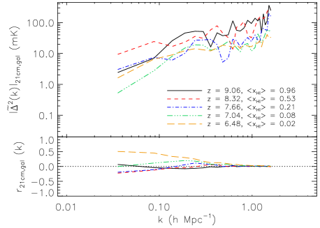
Figure 10: The circularly averaged, unnormalized 2D 21 cm – galaxy cross power spectrum (upper panel) and correlation coefficient (lower panel) for various redshifts/mean neutral fractions (see Fig. 4 for a legend) in our simulations in the LAE survey case. Slight differences in the cross power spectrum are seen for different redshifts.

We briefly revisit the effect of noise from the LOFAR instrument on our measurements. In Fig. 11 we repeat the comparison we made in Fig. 7. Here we find that at low redshift, while there is an intrinsic suppression of power on small scales, the noise serves to mask that effect. On large scales the noise decreases the power for both redshifts.

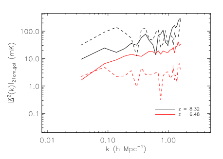
Figure 11: The circularly averaged, unnormalized 2D 21 cm – galaxy cross power spectrum calculated with (solid lines) and without (dashed lines) LOFAR noise in the LAE survey case. The addition of LOFAR noise makes it difficult to detect the suppression of power on small scales as the redshift decreases.

A LAE survey could yield useful information about the progress of reionization, but does it say anything about the topology of reionization? In Fig. 12 we return to our toy models and apply the same calculation machinery. The result is a somewhat clearer distinction between the two reionization scenarios. At scales of roughly $5h^{-1}\,{\rm Mpc}$, some difference is noted in the cross power spectrum while at larger scales significant differences in the correlation coefficient appear.

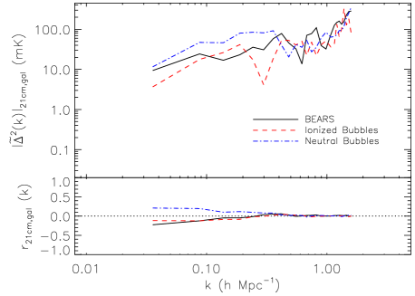
Figure 12: The circularly averaged, unnormalized 2D 21 cm – galaxy cross power spectrum (upper panel) and correlation coefficient (lower panel) for two toy models at $z=8.32$, $\langle x_{\rm\textsc{hi}}\rangle=0.53$ in the LAE survey case. It is possible to distinguish between the two ionization topologies using both the cross power spectrum and the correlation coefficient.

Finally, we consider four specific observing strategies for the Subaru Hyper-Suprime Cam (kindly provided to us by Masami Ouchi). The details are outlined in Table 3. Note that while there are deep and ultra-deep observations planned for the $z=6.6$ case, there is only an ultra-deep observation planned for the $z=7.3$ case. The current plan is to observe one of the $z=6.6$ deep fields with LOFAR, but here we consider all of the cases shown in Table 3.

Our outputs do not line up precisely with the redshifts for these planned observations, so we use the $z=6.48$ and $z=7.04$ outputs and expect that the difference would be minimal. Furthermore, we use a single slice of our simulation box to test the 3.5 and 4 square degree cases (corresponding to $\sim 40$ proper Mpc at $z=6.48$) and average 9 slices for the 28 square degree case (corresponding to $\sim 107$ proper Mpc at $z=6.48$). As for the estimates discussed earlier, we convert the Ly$\alpha$ luminosities to equivalent star formation rates using Equation 4.

The results are shown in Figs. 13 and 14 for $z=6.48$ and $z=7.04$, respectively. The first noticeable thing is that it makes little difference when the Ly$\alpha$ luminosity threshold or the observing area are changed by factors of a few. As we saw in the previous section, a major component in the shape of the curve is the LOFAR observing noise, not these two factors. Averaging over more fields does seem to smooth the curves slightly (although the curve in Fig. 14 is smoother only by chance), but it is not clear that using a deeper or wider field will improve the measurement significantly. If our fiducial reionization scenario is reasonable, these observations might be better performed at higher redshift in order to obtain a stronger 21 cm signal.

Table 3: Characteristics of four observing strategies with the Subaru Hyper-Suprime Cam.

Redshift	Number	Total area	$L_{\alpha,{\rm min}}$
	of fields	(square degrees)	(erg/s)
7.3	2	3.5	$1.3\times 10^{43}$
6.6	2	3.5	$2.8\times 10^{42}$
6.6	4	28	$6.2\times 10^{42}$
6.6	1	4	$6.2\times 10^{42}$

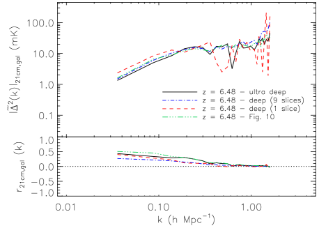
Figure 13: The circularly averaged, unnormalized 2D 21 cm – galaxy cross power spectrum (upper panel) and correlation coefficient (lower panel) for three specific Subaru Hyper-Suprime Cam observing strategies at $z=6.48$. Also shown by the solid line is the $z=6.48$ analysis from Fig. 10. Little difference is seen between the four curves.

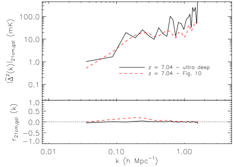
Figure 14: The circularly averaged, unnormalized 2D 21 cm – galaxy cross power spectrum (upper panel) and correlation coefficient (lower panel) for the Subaru Hyper-Suprime Cam observing at $z=7.04$. Also shown by the solid line is the $z=7.04$ analysis from Fig. 10. Little difference is seen between the two curves.

5 Conclusions

We have endeavoured to make predictions for the 21 cm – galaxy cross power spectrum. Using our bears code, we have performed radiative transfer simulations on the well-studied Millennium Simulation. Beginning with the spherically averaged dimensionless cross power spectrum between 21 cm emission and dark matter halos, we investigated how these two fields relate before attempting to make predictions for observations.

In general, we confirm the results of Lidz et al. (2009), who made their own predictions for the 21 cm – halo cross power spectrum. We find a similar shape and normalization, but owing to our coarser grid and poorer resolution, we find that at large $k$ our power spectrum shows oscillations related to the characteristic bubble size.

The 21 cm emission is initially correlated with halos on large scales, anti-correlated on medium, and uncorrelated on small scales. This picture changes quickly as reionization proceeds and the two fields become anti-correlated on large scales. Through toy models it becomes apparent that these correlations can be an useful tool for inferring the topology of reionization.

We then take the analysis in a different direction from Lidz et al. (2009). We attempt to make a more detailed mock observation of this signal in order to make predictions for upcoming surveys, using a well-studied semi-analytic model of galaxy formation and evolution (De Lucia et al., 2006) to bridge the gap between halos and galaxies. Applying the drop-out technique used in the Ouchi et al. (2009) survey severely reduced the number of galaxies at our disposal.

To further simulate the effect of observing and selecting real galaxies, we considered only a slab of our simulation box corresponding to the typical width of a filter. We then projected this slice and circularly averaged the power spectrum. We also added the noise expected from the LOFAR instrument to the 21 cm signal.

The result is that while the shape of the cross power spectrum is nominally preserved, its normalization seems to be the most powerful tool for probing reionization. In particular, it is sensitive to the ionized fraction as we show that different reionization histories yield similar cross power spectra for the same ionized fraction.

Compounding these problems is the fact that any galaxy survey will likely focus on a specific drop out range. We have seen that the cross power spectrum is quite useful when comparing the relative differences between different models or redshifts. In the absence of another redshift with which to compare results to, it might be troublesome to come up with a robust statement about reionization.

We turned to a more precise measurement of the galaxy redshifts that would be found using a LAE survey. We found that if the radial position of the galaxy is known, then much more information about the nature of reionization can be gleaned from cross-correlating the galaxy and 21cm fields. Using a LAE survey could in principle allow one to describe reionization using both the shape and normalization of the cross power spectrum.

A closer look at a specific planned LAE observing program using the Subaru Hyper-Suprime Cam reveals concerns about the strength of the 21 cm signal at the planned redshifts. If our estimate of the ionized fraction at $z=7$ is too high, then using the cross power spectrum might be a useful exercise given that at higher redshifts and neutral fractions it is able to distinguish between toy models with two different topologies. Indeed we predict that a detection of a correlation signal will be made - the main issue will be the interpretation of that signal.

There are a few observational effects which we have not included in our analysis. We have neglected to include peculiar velocities associated with both the galaxies and the IGM gas. On the galaxy side, we have neglected to mimic the effect of interlopers that could be misidentified as high-redshift galaxies. On the 21 cm side, we have assumed that the projected signal can be recovered on the angular scale of one of our resolution elements. A greater source of uncertainty however, may be the effect of foreground removal (e.g. Jelić et al., 2008; Bernardi et al., 2009; Harker et al., 2010; Jelić et al., 2010; Petrovic & Oh, 2011).

The prospect of combining upcoming galaxy surveys with measurements of the 21 cm signal remains quite exciting. Such combinations should not only be able to tell us about the progress of reionization, but the topology and the main drivers as well. This may turn out to be a key exercise in understanding this epoch while true imaging of 21 cm maps remains pending.

References

- Adshead & Furlanetto (2008) Adshead P. J., Furlanetto S. R., 2008, MNRAS, 384, 291
- Angulo & White (2010) Angulo R. E., White S. D. M., 2010, MNRAS, 405, 143
- Arons & Wingert (1972) Arons J., Wingert D. W., 1972, ApJ, 177, 1
- Becker et al. (2007) Becker G. D., Rauch M., Sargent W. L. W., 2007, ApJ, 662, 72
- Bernardi et al. (2009) Bernardi G., de Bruyn A. G., Brentjens M. A., Ciardi B., Harker G., Jelić V., Koopmans L. V. E., Labropoulos P., Offringa A., Pandey V. N., Schaye J., Thomas R. M., Yatawatta S., Zaroubi S., 2009, A&A, 500, 965
- Berndsen et al. (2010) Berndsen A., Pogosian L., Wyman M., 2010, MNRAS, 407, 1116
- Bolton & Haehnelt (2007) Bolton J. S., Haehnelt M. G., 2007, MNRAS, 382, 325
- Bouwens et al. (2008) Bouwens R. J., Illingworth G. D., Franx M., Ford H., 2008, ApJ, 686, 230
- Bouwens et al. (2012) Bouwens R. J., Illingworth G. D., Oesch P. A., Trenti M., Labbé I., Franx M., Stiavelli M., Carollo C. M., van Dokkum P., Magee D., 2012, ApJL, 752, L5
- Choudhury & Ferrara (2006) Choudhury T. R., Ferrara A., 2006, MNRAS, 371, L55
- Ciardi et al. (2011) Ciardi B., Bolton J. S., Maselli A., Graziani L., 2011, ArXiv e-prints
- Ciardi et al. (2000) Ciardi B., Ferrara A., Governato F., Jenkins A., 2000, MNRAS, 314, 611
- Ciardi et al. (2003) Ciardi B., Ferrara A., White S. D. M., 2003, MNRAS, 344, L7
- Dayal et al. (2008) Dayal P., Ferrara A., Gallerani S., 2008, MNRAS, 389, 1683
- De Lucia et al. (2006) De Lucia G., Springel V., White S. D. M., Croton D., Kauffmann G., 2006, MNRAS, 366, 499
- Dijkstra et al. (2007) Dijkstra M., Lidz A., Wyithe J. S. B., 2007, MNRAS, 377, 1175
- Dijkstra & Wyithe (2010) Dijkstra M., Wyithe J. S. B., 2010, MNRAS, 408, 352
- Fan et al. (2006) Fan X., Strauss M. A., Becker R. H., White R. L., Gunn J. E., Knapp G. R., Richards G. T., Schneider D. P., Brinkmann J., Fukugita M., 2006, AJ, 132, 117
- Furlanetto & Loeb (2005) Furlanetto S. R., Loeb A., 2005, ApJ, 634, 1
- Giavalisco et al. (2004) Giavalisco M., Ferguson H. C., Koekemoer A. M., Dickinson M., Alexander D. M., Bauer F. E., Bergeron J., Biagetti C., Brandt W. N., Casertano S., Cesarsky C., Chatzichristou E., Conselice C., Wolf C., 2004, ApJL, 600, L93
- Gnedin (2000) Gnedin N. Y., 2000, ApJ, 535, 530
- Harker et al. (2010) Harker G., Zaroubi S., Bernardi G., Brentjens M. A., de Bruyn A. G., Ciardi B., Jelić V., Koopmans L. V. E., Labropoulos P., Mellema G., Offringa A., Pandey V. N., Pawlik A. H., Schaye J., Thomas R. M., Yatawatta S., 2010, MNRAS, 405, 2492
- Hogan & Rees (1979) Hogan C. J., Rees M. J., 1979, MNRAS, 188, 791
- Iliev et al. (2006) Iliev I. T., Mellema G., Pen U.-L., Merz H., Shapiro P. R., Alvarez M. A., 2006, MNRAS, 369, 1625
- Jeeson-Daniel et al. (2012) Jeeson-Daniel A., Ciardi B., Maio U., Pierleoni M., Dijkstra M., Maselli A., 2012, ArXiv e-prints
- Jelić et al. (2010) Jelić V., Zaroubi S., Aghanim N., Douspis M., Koopmans L. V. E., Langer M., Mellema G., Tashiro H., Thomas R. M., 2010, MNRAS, 402, 2279
- Jelić et al. (2010) Jelić V., Zaroubi S., Labropoulos P., Bernardi G., de Bruyn A. G., Koopmans L. V. E., 2010, MNRAS, 409, 1647
- Jelić et al. (2008) Jelić V., Zaroubi S., Labropoulos P., Thomas R. M., Bernardi G., Brentjens M. A., de Bruyn A. G., Ciardi B., Harker G., Koopmans L. V. E., Pandey V. N., Schaye J., Yatawatta S., 2008, MNRAS, 389, 1319
- Kashikawa et al. (2004) Kashikawa N., Shimasaku K., Yasuda N., Ajiki M., Akiyama M., Ando H., Aoki K., Doi M., Fujita S. S., Furusawa H., Hayashino T., Iwamuro F., Yamada T., Yoshida M., 2004, PASJ, 56, 1011
- Kobayashi et al. (2007) Kobayashi M. A. R., Totani T., Nagashima M., 2007, ApJ, 670, 919
- Kohler et al. (2007) Kohler K., Gnedin N. Y., Hamilton A. J. S., 2007, ApJ, 657, 15
- Komatsu et al. (2011) Komatsu E., Smith K. M., Dunkley J., Bennett C. L., Gold B., Hinshaw G., Jarosik N., Larson D., Wright E. L., 2011, ApJS, 192, 18
- Leitherer et al. (1999) Leitherer C., Schaerer D., Goldader J. D., González Delgado R. M., Robert C., Kune D. F., de Mello D. F., Devost D., Heckman T. M., 1999, ApJS, 123, 3
- Lidz et al. (2011) Lidz A., Furlanetto S. R., Oh S. P., Aguirre J., Chang T.-C., Doré O., Pritchard J. R., 2011, ArXiv e-prints
- Lidz et al. (2009) Lidz A., Zahn O., Furlanetto S. R., McQuinn M., Hernquist L., Zaldarriaga M., 2009, ApJ, 690, 252
- Mao et al. (2011) Mao Y., Shapiro P. R., Mellema G., Iliev I. T., Koda J., Ahn K., 2011, ArXiv e-prints
- Muñoz & Loeb (2011) Muñoz J. A., Loeb A., 2011, ApJ, 729, 99
- Ouchi et al. (2009) Ouchi M., Mobasher B., Shimasaku K., Ferguson H. C., Fall S. M., Ono Y., Kashikawa N., Morokuma T., Nakajima K., Okamura S., Dickinson M., Giavalisco M., Ohta K., 2009, ApJ, 706, 1136
- Ouchi et al. (2010) Ouchi M., Shimasaku K., Furusawa H., Saito T., Yoshida M., Akiyama M., Ono Y., Yamada T., Ota K., Kashikawa N., Iye M., Kodama T., Okamura S., Simpson C., Yoshida M., 2010, ApJ, 723, 869
- Petrovic & Oh (2011) Petrovic N., Oh S. P., 2011, MNRAS, 413, 2103
- Raičević et al. (2011) Raičević M., Theuns T., Lacey C., 2011, MNRAS, 410, 775
- Razoumov et al. (2002) Razoumov A. O., Norman M. L., Abel T., Scott D., 2002, ApJ, 572, 695
- Salvaterra et al. (2005) Salvaterra R., Ciardi B., Ferrara A., Baccigalupi C., 2005, MNRAS, 360, 1063
- Schaye et al. (2010) Schaye J., Dalla Vecchia C., Booth C. M., Wiersma R. P. C., Theuns T., Haas M. R., Bertone S., Duffy A. R., McCarthy I. G., van de Voort F., 2010, MNRAS, 402, 1536
- Schroeder et al. (2012) Schroeder J., Mesinger A., Haiman Z., 2012, ArXiv e-prints
- Sokasian et al. (2003) Sokasian A., Abel T., Hernquist L., Springel V., 2003, MNRAS, 344, 607
- Springel et al. (2005) Springel V., White S. D. M., Jenkins A., Frenk C. S., Yoshida N., Gao L., Navarro J., Thacker R., Croton D., Helly J., Peacock J. A., Cole S., Thomas P., Couchman H., Evrard A., Colberg J., Pearce F., 2005, Nature, 435, 629
- Thomas & Zaroubi (2008) Thomas R. M., Zaroubi S., 2008, MNRAS, 384, 1080
- Thomas & Zaroubi (2011) Thomas R. M., Zaroubi S., 2011, MNRAS, 410, 1377
- Thomas et al. (2009) Thomas R. M., Zaroubi S., Ciardi B., Pawlik A. H., Labropoulos P., Jelić V., Bernardi G., Brentjens M. A., de Bruyn A. G., Harker G. J. A., Koopmans L. V. E., Mellema G., Pandey V. N., Schaye J., Yatawatta S., 2009, MNRAS, 393, 32
- Wright (2006) Wright E. L., 2006, PASP, 118, 1711
- Zahn et al. (2007) Zahn O., Lidz A., McQuinn M., Dutta S., Hernquist L., Zaldarriaga M., Furlanetto S. R., 2007, ApJ, 654, 12