A Cool Dust Factory in the Crab Nebula: a Herschel study of the filaments

Abstract

Whether supernovae are major sources of dust in galaxies is a long-standing debate. We present infrared and submillimeter photometry and spectroscopy from the Herschel Space Observatory of the Crab Nebula between 51 and 670 $\mu$m as part of the Mass Loss from Evolved StarS program. We compare the emission detected with Herschel with multiwavelength data including millimeter, radio, mid-infrared and archive optical images. We carefully remove the synchrotron component using the Herschel and Planck fluxes measured in the same epoch. The contribution from line emission is removed using Herschel spectroscopy combined with Infrared Space Observatory archive data. Several forbidden lines of carbon, oxygen and nitrogen are detected where multiple velocity components are resolved, deduced to be from the nitrogen-depleted, carbon-rich ejecta. No spectral lines are detected in the SPIRE wavebands; in the PACS bands, the line contribution is 5% and 10% at 70 and 100 $\mu$m and negligible at 160 $\mu$m. After subtracting the synchrotron and line emission, the remaining far-infrared continuum can be fit with two dust components. Assuming standard interstellar silicates, the mass of the cooler component is $0.24^{+0.32}_{-0.08}\,M_{\odot}$ for $\rm T=28.1^{+5.5}_{-3.2}\,K$. Amorphous carbon grains require $0.11\pm 0.01\,M_{\odot}$ of dust with $\rm T=33.8^{+2.3}_{-1.8}\,K$. A single temperature modified blackbody with $0.14\,M_{\odot}$ and $0.08\,M_{\odot}$ for silicate and carbon dust respectively, provides an adequate fit to the far-infrared region of the spectral energy distribution but is a poor fit at 24-500 $\mu$m. The Crab Nebula has condensed most of the relevant refractory elements into dust, suggesting the formation of dust in core-collapse supernova ejecta is efficient.

1. Introduction

In galaxies, the major dust source has in the past been presumed to be low-intermediate mass stars during their asymptotic giant branch (AGB) phase, but when accounting for dust destruction timescales (e.g. Jones 2001; Draine 2009) and the observed total dust masses, the required dust injection rate from stars can be an order of magnitude higher than observed (e.g. Matsuura et al. 2009; Gall et al. 2011; Dunne et al. 2011; Rowlands et al. 2012). An alternative source of dust is required to make up the dust budget (Pipino et al. 2011; Dunne et al. 2011). This shortfall in the dust mass estimated from AGB stars is also observed in dusty high-redshift galaxies where the timescales for dust production are close to, or shorter than, the lifetime of a typical low-mass AGB star (Morgan & Edmunds 2003; Dwek et al. 2007).

Significant dust production in supernova (SN) ejecta would alleviate these dust budgetary problems. SNe have long been proposed as a source of dust (e.g. Dwek & Scalo 1980; Clayton et al. 2001) yet subsequent mid and far-infrared (FIR) observations have detected only small quantities of warm dust in young ejecta (Sugerman et al. 2006; Meikle et al. 2011; Kotak et al. 2009; Andrews et al. 2011; Fabbri et al. 2011) and old remnants (Williams et al. 2006; Rho et al. 2008). These observed dust masses are orders of magnitude lower than required.

In the era of the Herschel Space Observatory (Pilbratt et al. 2010), we are now piecing together the relative contribution of stellar sources to the dust budget in galaxies, yet dust yields from the limited FIR studies of core-collapse remnants remain highly uncertain (Dunne et al. 2003; 2009; Krause et al. 2004; Barlow et al. 2010; Matsuura et al. 2011). Observations of historical Galactic remnants are important since these are (1) resolved, so that the different SN and interstellar/circumstellar tracers can be separated, and (2) young enough to ensure the thermal emission is not dominated by swept-up material. The Crab Nebula is one of only a few sources which satisfy these criteria and was chosen to be observed as part of the Herschel guaranteed time project Mass Loss from Evolved StarS (Groenewegen et al. 2011). This survey includes Cas A (Barlow et al. 2010) and the Type Ia remnants Kepler and Tycho (Gomez et al. 2012; see also Morgan et al. 2003 and Gomez et al. 2009). Unlike these remnants, the Crab has negligible cirrus contamination along the line of sight and is an ideal source to minimize the effects of unrelated interstellar material.

The Crab Nebula has been an object of interest for a number of years (see Hester 2008 for a comprehensive review). The remnant of an explosion in 1054 AD, the Crab is a pulsar wind nebula lying at a distance of 2 kpc (Trimble 1968). Its structure can be separated into two major components: the pulsar wind nebula (seen in X-rays and optical) with smooth synchrotron emission (at near-IR and radio wavelengths), and a network of filaments (traced in the optical and IR) consisting of thermal ejecta. The low expansion velocity of the ejecta suggests the remnant is the result of a Type II-P explosion (MacAlpine & Satterfield 2008). This is further confirmed by abundance constraints which put the progenitor star at $9$-$12\,M_{\odot}$ (Nomoto et al. 1982; Nomoto 1985; MacAlpine & Satterfield 2008).

Unusually amongst supernova remnants (SNRs), the material in the Crab is primarily photoionized by non-thermal radiation from the synchrotron nebula (e.g. Davidson & Fesen 1985; MacAlpine & Satterfield 2008). The latter authors found the main nebular gas component to be highly nitrogen-depleted and carbon-rich, although two other gas components with C/O $<1$ were also found to be present. The implication of this is that both carbon-rich and oxygen-rich dust species could exist in the nebula. Using optical data, Woltjer & Véron-Cetty (1987) detected the presence of absorption attributable to dust at the position of a bright [O iii] filament. Fesen & Blair (1990) obtained high angular resolution optical continuum images, revealing the presence of numerous “dark spots” across the synchrotron nebula coincident with bright emission cores seen in narrow-band [O i], [C i] and [S ii] images, consistent with dust existing in partially ionized or neutral clumps.

Previous IR studies confirmed the presence of dust grains in the Crab as early as the 1980s with masses ranging from $0.005$ to $0.03\,M_{\odot}$ (e.g. Marsden et al. 1984). Green et al. (2004) used ISO and SCUBA to infer the presence of $0.02$-$0.07\,M_{\odot}$ of dust depending on its composition. A careful analysis of the line contribution to the mid-IR using Spitzer data out to 70 $\mu$m suggested a dust mass of $0.001$-$0.01\,M_{\odot}$ (Temim et al. 2006). Using spatially resolved MIR spectroscopy across the remnant, Temim et al. (2012) later revised this to a silicate grain mass of $(2.4^{+3.2}_{-1.2})\times 10^{-3}\,M_{\odot}$.

Previous studies either lacked long wavelength spectroscopic information or adequate sampling of the FIR emission. In this paper, we present detailed FIR and crucially, submillimeter-through-to-millimeter observations of the Crab Nebula obtained with WISE, Spitzer, ISO, Herschel and Planck which allow us to accurately determine the synchrotron contribution and line emission to beyond 600 $\mu\rm m$. We can then estimate the total dust mass within the ejecta for the first time.

Inst.	RA, Decl. (J2000)	TDT/ObsID	Int. Time
Photometric Imaging
SPIRE	$\rm 05^{h}34^{m}31^{s}.97$, $22^{\circ}00^{\prime}52^{\prime\prime}.10$	1342191181	4555 s
PACS	$\rm 05^{h}34^{m}31^{s}.97$, $22^{\circ}00^{\prime}52^{\prime\prime}.10$	1342204441	1671 s
PACS	$\rm 05^{h}34^{m}31^{s}.97$, $22^{\circ}00^{\prime}52^{\prime\prime}.10$	1342204442	1671 s
PACS	$\rm 05^{h}34^{m}31^{s}.97$, $22^{\circ}00^{\prime}52^{\prime\prime}.10$	1342204443	1671 s
PACS	$\rm 05^{h}34^{m}31^{s}.97$, $22^{\circ}00^{\prime}52^{\prime\prime}.10$	1342204444	1671 s
Spectroscopy
ISO-1	$\rm 05^{h}34^{m}34^{s}.27$, $22^{\circ}01^{\prime}02^{\prime\prime}.4$	69501241	1124 s
ISO-2	$\rm 05^{h}34^{m}32^{s}.02$, $22^{\circ}02^{\prime}04^{\prime\prime}.6$	69301542	1126 s
ISO-3	$\rm 05^{h}34^{m}29^{s}.31$, $22^{\circ}00^{\prime}37^{\prime\prime}.0$	69301543	1124 s
ISO-4	$\rm 05^{h}34^{m}34^{s}.19$, $21^{\circ}59^{\prime}54^{\prime\prime}.7$	69301611	1630 s
FTS	$\rm 05^{h}34^{m}29^{s}.47$, $22^{\circ}00^{\prime}30^{\prime\prime}.4$	1342204022	3476 s
IFU	$\rm 05^{h}34^{m}29^{s}.44$, $22^{\circ}00^{\prime}32^{\prime\prime}.52$	1342217847	2267 s
IFU	$\rm 05^{h}34^{m}29^{s}.42$, $22^{\circ}00^{\prime}47^{\prime\prime}.17$	1342217847	1139 s

Table 1Observation Log for Herschel PACS and SPIRE Photometry and ISO LWS, Herschel PACS IFU, and SPIRE FTS Data Sets of the Crab Nebula.

2. Observations and data reduction

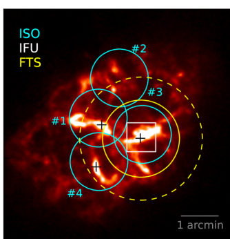
Figure 1.— $3\times 3$ arcmin region showing the Herschel PACS image of the Crab Nebula at 70 $\mu$m with the locations of the ISO LWS apertures (#1-4 –small cyan circles), PACS IFU (white rectangle) and SPIRE FTS FoV (yellow dashed). The unvignetted FTS FoV is also shown (solid yellow circle). Black crosses mark the locations of the Spitzer spectra from Temim et al. (2012).

2.1. Herschel Photometric Imaging

The Crab SNR was observed with the Herschel Photodetector Array Camera (PACS; Poglitsch et al. 2010) and Spectral and Photometric Imaging Receiver (SPIRE; Griffin et al. 2010) at 70, 100, 160, 250, 350 and 500 $\mu$m (a summary of the observations is listed in Table 1). The PACS photometry data were obtained in “scan-map” mode with speed 20 arcsec s^-1 including a pair of orthogonal cross-scans over 22 arcsec $\times$ 22 arcsec. In order to obtain images at all three PACS wavelengths, we used both the 70+160 $\mu$m and 100+160 $\mu$m channels, leading to the 160-$\mu$m image having twice the exposure time of the other two channels. The SPIRE maps are “Large Map” mode with scan length of 30 arcmin over 32 arcmin $\times$ 32 arcmin at a speed of 30 arcsec s^-1; a cross-scan is also taken, with a repetition factor of three. The data were processed following the description given in Groenewegen et al. (2011).

The PACS photometric data were reduced with the Herschel Interactive Processing Environment (HIPE; Ott 2010) applying all low-level reduction steps (including deglitching) to Level 1. The scanamorphos software (Roussel 2012) was then used to remove effects due to thermal drifts and uncorrelated $1/f$ noise of the individual bolometers and create the Level 2 map. The full width at half maximum (FWHM) at 70, 100, and 160 $\mu\rm m$ is 6, 8, and 12 arcsec, respectively. The flux calibration uncertainty for PACS is less than 10% (Poglitsch et al. 2010) and the expected color corrections are small compared to the calibration errors. We therefore adopt a 10% calibration error.

For SPIRE, the standard photometer pipeline (HIPE v.5.0) was used (Griffin et al. 2010) with an additional iterative baseline removal step (e.g. Bendo et al. 2010). The SPIRE maps were created with the standard naïve mapper (e.g. Griffin et al. 2008). We multiply the 350 $\mu$m data product by 1.0067 to be in line with the most recent calibration pipeline (v7). The FWHM for pixel sizes of 6, 10, and 14 arcsec is 18.1, 24.9, and 36.4 arcsec at 250, 350 and 500 $\mu\rm m$ respectively. The SPIRE calibration methods and accuracies are outlined by Swinyard et al. (2010) and are estimated to be 7%. The pipeline produces monochromatic flux densities for point sources but at the longer wavelengths, color corrections become significant and we therefore use the correction factors listed in the SPIRE Observer’s Manual (2011).

2.2. Herschel PACS and SPIRE Spectroscopy

A 51-210-$\mu$m full-range spectral scan was obtained with the PACS Integral Field Unit (IFU) Spectrometer (Poglitsch et al. 2010). The IFU has 5$\times$5 spaxels with each spaxel being 9.4 arcsec on a side. The coordinates (positioned on the brightest nebular filament - Figure 1), are listed in Table 1. The “chop-nod” spectrometer mode was used, with the “off” position located 6 arcmin to the north and south of the “on” position for the red and blue range scans, respectively. The “chop-nodded” observations contained one single nodding cycle and one single up-down scan in wavelength. The data were reduced to Level 2 products using the standard PACS chopped large range scan and spectral energy distribution (SED) pipeline in HIPE version 8.0.1 (Ott 2010) using calibration file PACS_CAL_32_0.

The SPIRE Fourier transform spectrometer (FTS) was used to obtain sparse-map spectra. Two bolometer arrays provided overlapping bands covering 32.0-51.5 cm^-1 (194-313 $\mu$m for the SPIRE Short Wavelength Spectrometer Array–SSW) and 14.9-33.0$\,\rm cm^{-1}$ (303-671$\,\rm\mu m$ for the SPIRE Long Wavelength Spectrometer Array–SLW). The SSW and SLW beamsizes are $\sim$18 and $\sim$37 arcsec, respectively. The two yellow circles in Figure 1 show the 2.2-arcmin diameter unvignetted and 3.2-arcmin diameter partially-vignetted field of view (FoV) for the SPIRE spectrometer pointing. A point-source calibration was applied to the central detectors of each array using Uranus (Swinyard et al. 2010). As the Crab is essentially fully extended in the beam, the calibration is modified using the self-emission of the telescope as the primary source (as we know both its temperature and emissivity properties). This telescope Relative Spectral Response Function is photometrically calibrated against Uranus using knowledge of the instrument spatial response function as described in the SPIRE Observers Manual (2011). The resulting spectra have an absolute calibration accuracy of 5% compared to the Uranus flux model of G. Orton et al. (in preparation).

2.3. ISO LWS Far-infrared Spectroscopy

In addition to our Herschel spectroscopy, we have made use of archival 43-197-$\mu\rm m$ spectra of the Crab obtained with the Long Wavelength Spectrometer (LWS; Clegg et al. 1996) aboard ISO. Figure 1 shows the positions of the four pointings of the LWS superposed on the PACS 70-$\rm\mu m$ image of the Crab (cyan circles – Table 1). The 44-110-$\rm\mu m$ parts of the spectra were previously published in Green et al. (2004). The data used here have been processed through the ISO-LWS Highly Processed Data Products pipeline (Gry et al. 2003) and further modified by removing gain shifts between the individual detectors using the central 100-$\rm\mu m$ detector as the reference. The Crab is relatively faint and the continuum spectrum beyond 150$\,\rm\mu m$ suffers from poor dark current removal and possible non-linear response in the detectors due to thermal instabilities. This portion of the continuum is considered untrustworthy although the line fluxes, in particular the [C ii] 158-$\rm\mu m$ line, are well calibrated.

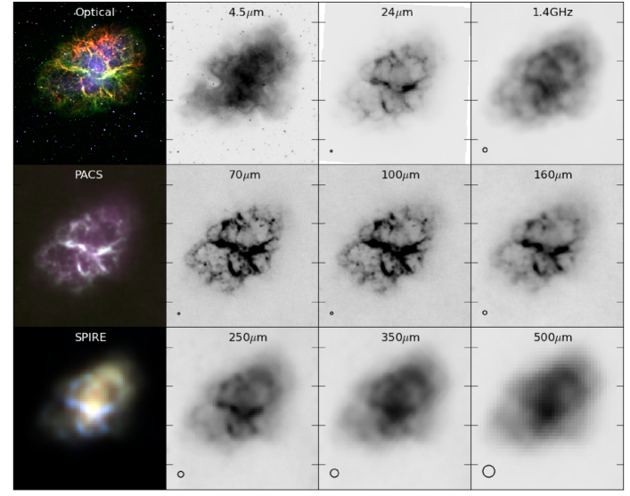
Figure 2.— Multiwavelength montage of the Crab SNR centered on the pulsar ($\rm R.A.=262^{\circ}.671$, $\rm decl.=22^{\circ}.0145$, J2000.0) with diameter $4^{\prime}.2\times 4^{\prime}.2$. Top: (from left to right): three color image in H$\alpha$ (red), [O iii] (green) and Bessel $B$ (blue) using images obtained from the Faulkes Telescope North (Appendix A). Spitzer IRAC 4.5 $\mu$m, MIPS 24 $\mu$m and VLA archive data at 1.4 GHz (taken in 1996). Middle: Herschel PACS three color image and individually the 70, 100 and 160 $\mu$m images. Bottom: Herschel SPIRE three color image and individually, 250, 350 and 500 $\mu$m images. Beam sizes are indicated with the black circle in the lower left corner.

The global integrated fluxes at the Herschel wavelengths are measured using an elliptical aperture with size $245\times 163^{\prime\prime}$ centered on the pulsar with the background contribution estimated using apertures off the remnant. These fluxes are combined with IR and submm fluxes from the literature as described in detail in Appendix A with photometric fluxes from 3.4 to 10,000 $\mu$m listed in Table 4 (see also Figures 4 and 5). These are combined with our own flux measurements at 3.4-22 $\mu$m with WISE and 3.6-70 $\mu$m Spitzer data (Appendix A).

When comparing the IR fluxes measured in this work (marked as “A” in Table 4) with the literature, we find that our PACS 70 $\mu$m flux for the Crab Nebula is significantly larger than the Spitzer measurement at the same wavelength (Temim et al. 2006). At first glance this appears to suggest a huge (40%) discrepancy between PACS and MIPS measurements (e.g., Aniano et al. 2012). However, we find this discrepancy disappears if we use the most recent calibration factors from Gordon et al. (2007). Re-reducing the 70 $\mu$m map using the most recent DAT instrument team pipeline produces a 70 $\mu$m flux of 210 Jy after the relevant color corrections are applied, this is in excellent agreement with our PACS measurement. Note that claimed differences between PACS and Spitzer MIPS can be resolved if instrumental effects are carefully considered; the PACS detectors are extremely stable with virtually no non-linearities compared to the Ge:Ga photoconductors employed in MIPS and indeed ISO. For these reasons, PACS has achieved an absolute calibration accuracy of 5% for point sources with $<10\%$ quoted here (compared to $~{}20\%$ for MIPS at 70 $\mu$m).

Since the radio synchrotron flux decreases with time by $-0.167\,\%\rm\,yr^{-1}$ (Aller & Reynolds 1985), radio fluxes measured at different epochs (Table 4) need to be corrected to the 2010 epoch to allow for comparison with the WISE, Herschel, and Planck data. Note that this “fading rate” assumes that the non-thermal fluxes decline at the same rate at all wavelengths.

3. Disentangling the contributions from different components

In Figure 2, we present a multiwavelength view centered on the Crab, comparing the Herschel PACS and SPIRE images with synchrotron emission seen at near-IR (with Spitzer IRAC) and at radio wavelengths with the Very Large Array (VLA), and the ionized gas observed at optical wavelengths. The smooth non-thermal synchrotron emission seen at 4.5 $\mu$m appears to be confined within the filamentary structures seen in optical and IR wavebands which originate from ionized gas and dust emission. Previous works have shown that the warm dust component (seen in emission at 24 $\mu$m) traces the densest gas in the cores of filaments in low ionization states (e.g., [O i] - Blair et al. 1997; Loll et al 2007) and this is confirmed by the filamentary emission seen in the MIPS and Herschel PACS images. The distribution of the emission in the Herschel SPIRE 250 $\mu$m image is similar to the shorter IR wavelengths. At the longer SPIRE wavelengths (Figure 2), we start to see a strong resemblance with the radio emission at 1.4 GHz, which traces both the smooth synchrotron seen at the shorter 4.5 $\mu$m band, but also some filamentary emission arising from free-free emission (e.g. Temim et al. 2006). While the free-free emission only makes a negligible contribution to the FIR continuum for the Crab (see Appendix B), the synchrotron component and line emission are important at these wavelengths and need to be removed before we can investigate if there is residual emission from dust.

3.1. Line Emission

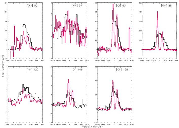
Figure 3.— Velocity profiles of the emission lines detected in the Crab Nebula using the coadded PACS spectra (red) and the LWS spectrum (black) taken at the same location (#3). The text in the top right corner lists the approximate central wavelength of the lines which at $51.8145\,\mu$m and 88.3564 $\mu$m for [O iii] (NIST Atomic Spectra Database); 63.18371$\mu$m and 145.5255 $\mu$m for [O i] (Zink et al. 1991); 157.74095 $\mu$m for [C ii] (Cooksy et al. 1986); and 121.8976 $\mu$m and 205.1783 $\mu$m for [N ii] (Brown et al. 1994).

Temim et al. (2012) present a comprehensive analysis of the MIR spectral lines across the Crab Nebula, with a number of forbidden lines identified up to 36 $\mu$m. They estimate that the contribution of line emission to the 24 $\mu$m broadband flux is 27%, 54%, and 48% measured at different locations across the remnant (shown in Figure 1), suggesting on average, that line emission contributes 43% $\pm$ 6% of the flux (Table 2). (The error quoted in this average is simply the range of values obtained on the dense filaments.) Note that this estimate of the line contribution was obtained after Temim et al. subtracted synchrotron emission from the Spitzer map.

$\lambda$	Line Contribution in Band (%)
($\mu$m)					Average
24	…	54	48	27	43 $\pm$ 6a
	#1	#2	#3	#4
70	6.6	4.2	5.4	4.4	4.90 $\pm$ 0.05b
100	12.9	5.6	9.6	6.7	8.7 $\pm$ 0.3b

Table 2The contribution to the total integrated flux at 24, 70 and 100 $\mu$m at different locations across the remnant (Figure 1). ^a - This represents the contribution of line emission to the flux after synchrotron subtraction has been carried out (Temim et al. 2012). ^b - The contribution at 70 and 100 $\mu$m from line emission estimated using ISO LWS and Herschel PACS.

In order to determine the contribution of line emission to the broad band infrared fluxes of the Crab Nebula, Herschel PACS and SPIRE, and ISO LWS data were analyzed. Figure 3 shows the velocity profiles of the seven emission lines detected in the co-added Herschel PACS spectra and in the LWS spectrum taken at the same location. Although the LWS line profiles are significantly broadened compared to the instrumental resolution, it requires the higher PACS spectral resolutions to fully resolve the individual blueshifted and redshifted velocity components from the ejecta. The separations between the blue and red component emission peaks vary between 1290 and 1750$\rm\,km\,s^{-1}$, depending on the species (the profiles will be discussed further in a separate paper).

The seven emission lines and their gas properties are discussed fully in Appendix C with fluxes measured relative to the [O iii] line provided in Table 5. These lines suggest the Crab Nebula ejecta is nitrogen-depleted and carbon-rich (unlike Cas A; Rho et al. 2008) implying that the dust is likely to be carbon-rich. However, there is also evidence that some regions in the Nebula have solar-like CNO abundances which may allow silicate-type grains to also form (see Appendix C for more details).

The four LWS spectra were used to estimate the contributions from the emission lines to the measured PACS 70 and 100 $\mu\rm m$ broad-band fluxes. To do this, the PACS filter spectral response functions were convolved with and integrated across (1) the observed LWS spectra, including emission lines; and (2) the LWS spectra after excising emission lines and interpolating the adjacent continua across the positions of the lines. The mean ratio of the case (2) to case (1) in-band fluxes was found to be 0.951$\pm$0.012 for the 70 $\mu\rm m$ filter and 0.913$\pm$0.028 for the 100 $\mu$m filter (Table 2). We have applied these average line correction factors to the measured 70- and 100-$\mu$m fluxes to obtain the continuum-only broadband fluxes. The 146 and 158 $\mu\rm m$ emission lines (Table 5) contribute a negligible amount to the broad-band PACS 160 $\mu\rm m$ flux measurement. No emission lines were detected in any of the spectra from the SPIRE FTS detectors, the contribution of line emission to the broad-band SPIRE photometry is therefore negligible.

3.2. Synchrotron Emission

In this section, we now estimate the contribution from the non-thermal synchrotron component. To do this, we fit a power law to the Spitzer IRAC, WISE and Planck data (large circles in Figure 5).

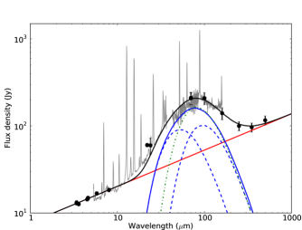
Figure 4.— IR SED of the Crab Nebula including the integrated fluxes from Herschel, the new Spitzer calibration and WISE fluxes (black points). The errors include the photometric errors (dominated by calibration errors, Table 4), the error in the synchrotron extrapolation and the error in the line emission contribution (Table 2) added in quadrature. The ISO #3 spectra scaled to the 100 $\mu$m flux is overplotted in gray. The average (dereddened – see Indebetouw et al. 2005) Spitzer spectroscopy (from the two brightest filaments in Figure 1) is overplotted for comparison. The synchrotron power law is shown in red. Two temperature components of amorphous carbon dust at 63 and 34 K required to fit the SED are plotted (blue dashed) with the sum of these plotted in solid blue. A single-temperature amorphous carbon fit (40 K) to the FIR is also shown (green dot-dashed). The sum of the two-component dust and synchrotron contributions is shown by the solid black curve.

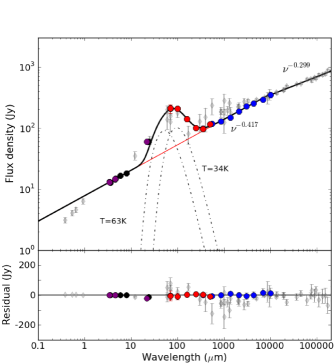
Figure 5.— SED of the Crab Nebula from the IR-radio including Herschel (red points) and Spitzer (black), WISE (purple) photometry and Planck fluxes (Planck Collaboration 2011, blue points). Previous fluxes from the literature (see Table 4 and references therein) are shown with gray diamonds. The synchrotron law fitted to the $3.6-10^{4}\,\mu$m data points is the dashed black line. Dot-dashed lines are the fitted components from thermal emission by amorphous carbon grains (see Figure 4). The solid black line is the total flux obtained from summing the synchrotron and the two dust components (with the residual shown below). Note the total integrated fluxes plotted here also include a contribution from line emission at 24, 70, and 100 $\mu$m (Section 3.1), which has not been added to the total black SED curve plotted here.

Including the Planck fluxes in the SED allows us to fully constrain the synchrotron power law between 3.4 $\mu$m and 1 cm for the first time, using observations taken at the same epoch. A least-squares fit to the Spitzer-WISE-Herschel-Planck data set produces a power law with frequency dependence $\nu^{-0.417}$ and amplitude 1489 Jy at 1 GHz (Figure 5). The error in the synchrotron spectral index ($\alpha$) from the line of best fit is $\pm 0.006$. Extrapolating the expected fluxes at the IR-submm wavebands due to synchrotron emission using the integrated fluxes for the remnant with the above power law, we estimate the synchrotron flux in each waveband (Table 4).

The synchrotron power law in the FIR regime derived in this work is steeper than the slope determined in the review by Macías-Pérez et al. (2010), where the extrapolation to the submm from the longest radio wavelengths suggested one synchrotron component with $\alpha=-0.3$. We argue here that the exquisite coverage between the IR and radio regime given by Herschel SPIRE and Planck suggests that the synchrotron emission is described by (at least) two power laws, with wavelengths beyond $10^{4}$ $\mu$m (30 GHz), following the flatter relationship $\nu^{-0.3}$ (as also seen in Green et al. 2004; Arendt et al. 2011). The slope then breaks, becoming the steeper $\nu^{-0.42}$ law we find here. In fitting this synchrotron power law, we do not incorporate the previous literature data obtained in the submillimeter-millimeter regime (shown by the faint gray diamonds in Figure 5) since these fluxes often have large calibration errors, with small FoVs. One should be particularly cautious when using the ISOPHOT data of the Crab (Green et al. 2004) since this was obtained in P32 chopping mode, which can suffer significantly from transient effects with unreliable calibration (U. Klaas, private communication). This dataset was never released as a scientifically validated measurement and therefore the quoted calibration accuracy for ISOPHOT (30%) is not applicable for this dataset. The previous literature measurements were also taken at different epochs and corrected using the average “fading” rate (Appendix A). With WISE, Herschel, and Planck, not only are the photometric errors less than 10%, the images also have a large background area to sample and the data were taken at the same epoch, therefore not relying on the application of a correction factor.

It is possible that the synchrotron spectrum could further break into different components in the IR regime (as suggested by Arendt et al. 2011) which would introduce further errors on the amount of synchrotron estimated at each wavelength. However, we see no evidence for a sharp break either via the presence of excess flux or in differences in the spectral index maps created from the IRAC bands versus maps created from the VLA-Herschel images. Unfortunately, given the low angular resolution in the FIR/submm, any local variations in the spectral index would not be seen in the method we have used in this work. The present data are therefore insufficient to separate out any small-scale variations in the synchrotron slope which may account for some of the residual emission. The shape of the SED at wavelengths beyond 70 $\mu$m and the Planck coverage rules out a significant break in the FIR/submm regime at least. However, we note that the flux attributed to synchrotron could be underestimated at 24 $\mu$m if there is a break to a steeper power law at wavelengths less than 70 $\mu$m.

In order to spatially determine the distribution of synchrotron and excess thermal emission from dust, we follow Temim et al. (2006) who used a combination of the Spitzer IRAC and radio images to obtain a spectral index map. We repeat this procedure using the extinction-corrected 4.5 $\mu$m IRAC image and the 500 $\mu$m Herschel SPIRE map, both of which are completely dominated by synchrotron emission. After aligning and convolving the IR-submm images, we re-grid them to the same pixel size and deconvolve our spectral index image with the appropriate beam. We use the deconvolved spectral index map to subtract the extrapolated synchrotron flux expected at each IR-submm waveband using the spectral index for that pixel. In Figure 6 we show the extrapolated synchrotron emission expected at 24 $\mu$m using the spectral index map made in this way. Note that the subtraction of the synchrotron component on a pixel-by-pixel basis removes the smooth emission at 24 $\mu$m seen in Figure 2, leaving only the excess filamentary emission originating from the warm dust component.

3.3. Thermal Emission from Dust

Using the global SED of the Crab (Figures 4 and 5), after removing the contribution from line emission and the well-constrained synchrotron component, we find the excess thermal emission observed in the FIR can be described by the sum of two modified blackbodies arising from a warm ($T_{w}$) and a cool ($T_{c}$) component. Although we would expect a more complex temperature distribution for dust in the remnant, a two-temperature component fit is adequate for a first-order approach in modeling the SED. We can then fit the data with optical constants appropriate for silicate or carbon grains, with the dust mass estimated using Equation (1). $S_{\nu}$ is the flux density, $D$ is the distance, $B(\nu,T)$ is the Planck function and $\kappa_{\nu}$ is the dust mass absorption coefficient calculated from the dust emissivity $Q_{\nu}$ (for silicates – Weingartner & Draine 2001), and the grain density $\rho$ (Laor & Draine 1993):

$$M_{d}={S_{\nu}D^{2}\over{\kappa_{\nu}}B(\nu,T)}.$$ (1)

The total dust mass from the FIR model (see Table 3) for astronomical silicates is dominated by the cool component which requires a best-fit temperature of $T_{c}=\rm 28.1^{+5.5}_{-2.8}\,K$ and mass $M_{d}=0.24^{+0.32}_{-0.08}\,M_{\odot}$. The warm component (Figure 4) arises from $(8.3^{+3.6}_{-6.4})\times 10^{-3}\,M_{\odot}$ of dust at a temperature of $\rm 55.6^{+7.8}_{-2.8}\,K$.

As the gas in the filaments is carbon-rich (Appendix C), the dust may be composed of amorphous carbon grains. In this case (with $Q_{\nu}$ taken from Zubko et al. 1996 (their ‘BE’ model) and $\rho$ from Rouleau & Martin 1991), the dust mass arising from the cool component reduces to $0.11\pm 0.01\,M_{\odot}$ with $T_{c}=\rm 33.8^{+2.3}_{-1.8}\,K$. The warm component requires only $M_{d}=(6.0^{+1.1}_{-2.4})\times 10^{-3}\,M_{\odot}$ at $T_{w}=63.4^{+5.1}_{-2.7}\,\rm K$.

We also attempted to fit iron grains to the SED (following Matsuura et al. 2011) yet it is difficult to fit the MIR part of the thermal emission. To explain the FIR emission (i.e. beyond 70 $\mu$m) with iron grains, we require $\sim 0.3\,M_{\odot}$ of dust at temperatures 34 and 69 K with radius $0.1\,\mu$m (where $Q_{\nu}$ is taken from Semenov et al. 2003 and $\rho$ from Nozawa et al. 2006). However, the mass of iron grains is highly dependent on the grain size, for example grains with radius $<0.005\,\mu$m would require more than $70\,M_{\odot}$ of dust.

We attempted to fit the residual emission from 24 to 350 $\mu$m with a single-temperature modified blackbody, producing the parameters $M_{d}\sim 0.14\,M_{\odot}$ with $T\sim\rm 34\,K$ for astronomical silicates and $M_{d}\sim 0.08\,M_{\odot}$ with $T\sim\rm 40\,K$ for amorphous carbon (the green dot-dashed curve in Figure 4). However, the single component always severely underestimates the flux at 24 $\mu$m. For this to be explained via contamination of line emission in this waveband, we would require 96% of the broad-band flux at 24 $\mu$m to be due to line contribution; this is clearly not supported by the careful analysis of IR spectra across the remnant in Temim et al. (2012). Given that the two-component model adequately fits the entire IR-submm SED and that the chi-squared statistic favors a two-component model fit (Table 3), we suggest this is the most valid model for the data. Ultimately, the difference in the final mass is small whether one or two dust populations exist if the grains are carbon-rich though the silicate dust mass estimated from the single-temperature fit is reduced by approximately half.

	Two-component Model
	Warm Component		Cool Component
	$T_{w}$ (K)	$M_{d}$ ($\times 10^{-3}M_{\odot}$)	$T_{c}$ (K)	$M_{d}$ ($M_{\odot}$)	$\chi^{2}$
Si	$55.6^{+7.8}_{-2.8}$	$8.3^{+3.6}_{-6.4}$	$28.1^{+3.2}_{-5.5}$	$0.24^{+0.3}_{-0.1}$	0.05
C	$63.4^{+5.1}_{-2.7}$	$6.0^{+1.1}_{-2.4}$	$33.8^{+2.3}_{-1.8}$	$0.11\pm 0.01$	0.23
	One-component Model
	$T_{d}$ (K)	$M_{d}$ ($M_{\odot}$)	$\chi^{2}$
Si	34	0.14	$3\times 10^{-5}$
C	40	0.08	$7\times 10^{-3}$

Table 3Summary of the best-fit dust masses and temperatures for silicate and amorphous carbon grains using the two (top) and one (bottom) component dust models displayed in Figures 4 and 5. Note: the reduced $\chi^{2}$ statistic is also included.

Note that modeling the SED with dust grains with a continuous temperature distribution could produce a lower dust mass compared to that estimated using the two-temperature approach. The dust masses quoted in Table 3 should then be regarded as an upper limit on the mass of dust in the remnant. However the largest uncertainty in a quoted dust mass arises from the choice of optical constant. This becomes more important when choosing models within the “umbrella” term amorphous carbon, which encompasses a number of different classes of materials such as soot, glassy carbon (Jägeret al. 1998), and the ACAR/ACH2/BE models of amorphous grains from Zubko et al. (1996). Although the optical constants vary depending on which of these grain types is chosen, at FIR wavelengths $Q_{\nu}$ varies by only a factor of a few for these different types (Figure 10 in Jäger et al. 1998; Hanner 1988). One exception to this arises if the grains are pyrolyzed cellulose where $Q_{\nu}$ is different by a factor of 10 (Jäger et al. 1998).

The distribution of the warm dust component is shown in Figure 6 using the synchrotron- and line emission-subtracted 24 $\mu$m image. We can now use this warm dust map to extrapolate the expected emission from the warm dust component in the Herschel bands and reveal the distribution of the cool dust component. The spatial distribution of the synchrotron emission at 160 $\mu$m (using the spectral index map) is shown in Figure 6 along with the extrapolated warm and cool dust components at this wavelength. The morphology of this cool dust is similar to the warm dust emission at 24 $\mu$m and is distributed in the dense filamentary structures as expected.

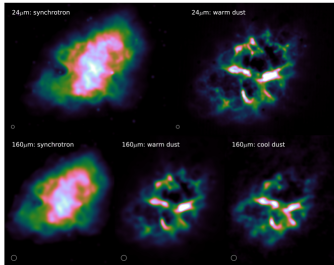
Figure 6.— Top: the distribution of synchrotron and thermal emission from the warm dust component at 24 $\mu$m. Bottom: the Herschel SPIRE 160 $\mu$m emission separated into the synchrotron component (left), the warm dust component (as traced by the emission at 24 $\mu$m) (middle) and the newly identified cool dust component (right). The color palette used in the online version of this figure is the cubehelix scheme in which color monotonically increases in terms of perceived brightness (Green 2011).

4. Dust in the Crab Nebula

Using Spitzer data out to 70 $\mu$m, Temim et al. (2012) derived a silicate grain mass of $2.4\times 10^{-3}\,M_{\odot}$ ($T\sim 55\,\rm K$) and $3.2\times 10^{-3}\,M_{\odot}$ ($T\sim 60\,\rm K$) for carbon grains. Their estimates are of similar order to the mass of grains estimated from the hot component listed in Table 3. However, the total dust mass derived here is at least an order of magnitude higher than Temim et al. with $M_{d}\sim 0.24\,M_{\odot}$ ($T_{c}\sim 28\,\rm K$) or $0.11\,M_{\odot}$ ($T_{c}\sim 34\,\rm K$) for silicates and carbon grains. The difference in mass between these two studies is not due to the optical constants assumed, since Temim et al. use the ACAR model from Zubko et al. (1996) which has similar $Q_{\nu}$ to the BE model used here at FIR wavelengths. The difference is due to the longer wavelength coverage of Herschel PACS and SPIRE, the matched-epoch observations and careful subtraction of synchrotron emission in the FIR–submillimeter regime.

To account for their dust temperature of $50$–$60\,\rm K$, Temim et al. (2012) modelled the dust heating (via non-thermal radiation) and cooling rates (through IR emission) in the Nebula. They showed that the IR emission ($\lambda<70\,\mu\rm m$) originates from small grains with radii $<0.015\,\mu$m. Their results imply that the SN grains in the Crab are small, and therefore easier to destroy via sputtering; the authors also point out that this is somewhat at odds with theoretical models of SN grain formation (e.g. Kozasa et al. 2009). Given the newly detected cool dust component in this work, the long-wavelength radiation originates from larger grains with radius $>0.06\,\mu$m. Such grains are predicted by the Kozasa et al. model and would suggest this new cool component of dust would be harder to destroy.

Since the dust is spatially coincident with ionized ejecta material (Figure 3), it is plausible that the thermal emission arises from newly formed grains. Indeed, we can rule out a swept-up interstellar origin using a simple argument (see, for example, the Tycho and Kepler remnants–Gomez et al. 2012). The volume swept up by the Crab is $\sim 15\,\rm pc^{3}$, sweeping up a total gas mass of approximately one-tenth of a solar mass (Trimble 1970; Davidson & Fesen 1985) for typical interstellar densities. Applying a standard gas-to-dust ratio (Devereux & Young 1990), the swept-up dust mass would therefore be $<10^{-2}\,M_{\odot}$. At the location of the Crab (180 pc above the Galactic plane), the interstellar density is thought to be much less than the canonical value, indeed the surrounding medium appears devoid of material (Davidson & Fesen 1985), placing even more stringent constraints on the possibility that the dust here is swept up material.

Are the dust masses estimated here sensible given the expected heavy element abundances from the SN? The total amount of heavy elements (and therefore the mass available to form dust) in the SN ejecta from a $9$–$12\,M_{\odot}$ progenitor star varies from $0.2$ to $0.5\,M_{\odot}$ depending on the model used and the mass of the progenitor (Maeder 1992; Woosley & Weaver 1995; Limongi & Chieffi 2003; Nomoto et al. 2006). The limit on the abundances expected in the ejecta from these theoretical models provides the constraint for the maximum possible dust mass, these are 0.09 $M_{\odot}$ for carbon, 0.03 $M_{\odot}$ for MgO, and 0.04 $M_{\odot}$ for $\rm SiO_{2}$. For silicate-rich grains, we can increase the available mass to $0.19\,M_{\odot}$ if we allow iron to form grains, for example including grain compositions such as $\rm FeSiO_{3}$.

From the elemental abundances constraint, both the silicate and carbon dust masses estimated from the SED fitting are well within the maximum possible dust masses allowed for these compositions. Whether the grains are silicate- or carbon-rich, the observed dust masses suggest efficient condensation of metals in the filaments.

5. Conclusions and Discussion

The combination of Spitzer, WISE, ISO, Herschel, Planck photometry and spectroscopy at longer wavelengths than probed before, reveals a previously unknown cool dust component in the Crab Nebula located along the ionized filamentary structures.

To reveal this new dust component, we carefully removed the synchrotron component using WISE, Herschel and Planck fluxes for the remnant measured in the same epoch. We find a steeper $\nu^{-0.417}$ power-law variation with frequency for the non-thermal component which describes the emission from synchrotron at wavelengths of 3.4–10,000 $\mu$m.

The contribution from line emission is then removed using Spitzer IR spectroscopy (Temim et al. 2012) and our analysis of Herschel spectroscopy combined with ISO LWS archive data. FIR spectroscopy yields high O/N ratios and although appears to be carbon-rich, also has a component with solar-like CNO abundances. It seems likely that carbon and silicate grains could be located in the ejecta.

The mass of dust estimated using the two-temperature approach to fitting the SED ranges from $0.1$ to $0.2\,M_{\odot}$ depending on whether the grains are composed of amorphous carbon or astronomical silicates respectively. The warm and cool dust components are distributed in the filaments coinciding spatially with Doppler-shifted ejecta material (traced via spectroscopy). This indicates the dust is spatially coincident with the ejecta material and not swept up circumstellar/interstellar material.

Comparing with the expected elemental abundances in the ejecta, this work suggests the condensation of heavy elements into dust grains is efficient, and that the filaments may provide a viable environment to protect the dust from shocks. The dust mass estimated for the Crab in this work is similar to the cool (unambiguously) associated SN dust mass observed in Cas A, and at the lower limit of the mass estimated in SN1987A using recent Herschel observations (Matsuura et al. 2011). Todini & Ferrara (2001) and Kozasa et al. (2009) predict between $0.1$ and $0.3\,M_{\odot}$ of dust should form in the ejecta from the (Type-IIP) explosions of progenitor stars with initial mass $<15\,M_{\odot}$, in agreement with the dust masses derived here.

It is unclear how much of the newly formed ejecta dust will survive. Grains will be destroyed via thermal sputtering in the reverse shock due to collisions with electrons and/or ions, yet unlike the Cas A and SN1987A remnants, the Crab does not have a visible reverse shock today (Hester 2008). The current environment in which the dust particles find themselves in appears relatively benign, as shown by the large amounts of molecular hydrogen comfortably surviving within the filaments (Graham et al. 1990; Loh et al. 2011). The dust particles in the Crab Nebula appear well set to survive their journey into the interstellar medium and contribute to the interstellar dust budget. Future ALMA observations of this source and other remnants are crucial to disentangle synchrotron and dust emission on smaller scales. This will be particularly important in comparing the time evolution of dust forming and being destroyed in remnants at different stages.

Appendix A Ancillary Data

We used 3.6–70 $\mu$m data from Spitzer IRAC and MIPS (PI. R. Gerhz; Temim et al. 2006). The fluxes were corrected for extended emission and color correction. Calibration uncertainties were assumed to be 5% for IRAC and 10% at 24 and 70 $\mu$m and we applied the most up-to-date calibration factors from Gordon et al. (2007).

We obtained single exposure (level 1b) images of the WISE (Wright et al. 2010) all-sky release through the NASA/IPAC Infrared Science Archive at 3.4, 4.6 and 22 $\mu$m. Montage was used to process and co-add the single exposure images. Median filtering of the single exposure frames was used to make basic cosmetic corrections. Calibration factors were applied according to the WISE Explanatory Supplement with photometric errors assumed to be 5% (see e.g Mainzer et al. 2012).

For comparison purposes, we use optical images of the Crab (Figure 2) using the 2.0 m Faulkes Telescope North on in H$\alpha$ (200 s) and [O iii] narrowband filters (240 s) and the broad-band Bessel blue filter (200 s).

Photometric fluxes measured in previous works were added to the Herschel and Spitzer datasets presented here, including fluxes from Planck (Planck Collaboration 2011), archeops (Macías-Pérez et al. 2010), theKuiper Airborne Observatory (Wright et al. 1979), IRAS (Strom & Greidanus 1992), ISOPHOT and SCUBA (Green et al. 2004). The fluxes listed in Table 4 that were not measured in this work, were taken from the compilation of literature fluxes in Macías-Pérez et al. (2010), Arendt et al. (2011), or from the Planck archive. In this work, we adopt calibration errors of $15\%$ for IRAS. For the ISOPHOT data, we can only assume a calibration error of 30% which is appropriate for scientifically valid datasets (from mode P22, for example). However, the Crab data have not been scientifically validated so this is a lower limit on the flux error.

$\lambda$	Epoch	$S_{\rm tot}$	Error	$S_{\rm synch}$	Inst.	Ref.
($\mu$m)		(Jy)	(Jy)	(Jy)
3.4	2010	12.9	0.6	13.1	WISE	A
3.6	2004	12.6	0.22	13.2	Spitzer	a
4.5	2004	14.4	0.26	14.5	Spitzer	a
4.6	2010	14.7	0.75	14.6	WISE	A
5.8	2004	16.8	0.1	16.1	Spitzer	a
8.0	2004	18.3	0.13	18.5	Spitzer	a
22	2010	60.3	3.5	28.1	WISE	A
24	2004	59.8	6.0	29.2	Spitzer	a
…	2004	59.3	5.9	…	Spitzer	A
60	1998	140.7	42.4	42.8	ISO	b
…	1983	210.0	8.0	…	IRAS	c
70	2004	208.0	33.3	45.6	Spitzer	A
…	2010	212.8	21.3	…	Herschel	A
100	1998	128.2	38.5	52.9	ISO	b
…	1983	184.0	13.0	…	IRAS	c
…	2010	215.2	21.5	…	Herschel	A
160	2010	141.8	14.2	64.3	Herschel	A
170	1998	83.2	26.5	66.0	ISO	b
250	2010	103.4	7.2	77.5	Herschel	A
300	1979	135.0	41.0	83.6	KAO	d
350	2010	102.4	7.2	89.2	Herschel	A
…	2010	99.3	2.4*	…	Planck	f
400	1979	158.0	63.0	94.3	KAO	d
432	2007	224	24	97.4	IRAM	e
500	2010	129.0	9.0	103.5	Herschel	A
550	2010	117.7	2.1*	107.7	Planck	f
-	2002	237.0	68.0	…	Archeops	g
850	2002	186.0	34.0	129.0	Archeops	g
…	2010	128.6	3.1*	..	Planck	f
…	1999	190.0	19.0	…	SCUBA	b
1000	1979	131.0	42.0	138.1	CH	d
…	1983	194.0	19.0	…	Mt. Lemmon	h
…	1976	300.0	80.0	…	Hale	i
1382	2010	147.2	3.1*	158.1	Planck	f
2098	2010	187.1	2.0*	188.1	Planck	f
3000	2010	225.4	1.1*	218.4	Planck	f
4286	2010	253.6	2.5*	253.4	Planck	f
6818	2010	291.6	1.3*	307.5	Planck	f
10000	2010	348.2	1.2*	360.7	Planck	f

Table 4Integrated fluxes for the Crab Nebula.
Notes: Also included are the synchrotron fluxes derived from $\nu^{-0.417}$.
References: A - this work; a - Temim et al. (2006); b - Green et al. (2004); c - Strom & Greidanus (1992); d - Wright et al. (1979); e - Arendt et al. (2011) f - Planck Collaboration 2011; g - Macías-Pérez et al (2010); h - Chini et al. (1984); i - Werner et al. (1977). * - These errors are the uncertainty in flux quoted in the Planck catalog which does not include calibration errors ($<7\%$). CH - University of Chicago photometer. KAO - Kuiper Airborne Observatory.

Appendix B Contribution from Free–Free Emission

Using a simple argument we can demonstrate that free–free radiation makes a negligible contribution to the 200 -$\mu$m continuum flux of the Crab Nebula.

An upper limit can be derived starting from observed $F({\rm H}\beta)$ values (taken here to be $1.78\times 10^{-11}\rm\,erg\,cm^{-2}\,s^{-1}$ from MacAlpine & Uomoto 1991). They also measure a global $F(5876{\rm\AA})/F({\rm H}\beta)\sim 0.84$, while Davidson (1987) measured $F(4686{\rm\AA})/F({\rm H}\beta)\sim 0.74$ and Smith (2003) measured $\sim 0.72$ giving a mean ratio of 0.73. De-reddening these ratios with $E(B-V)=0.47$, adopting a mean temperature ($T_{e}\sim 9000$ K) and using standard recombination emissivities, gives $n({\rm He}^{+})/n({\rm H}^{+})=0.44$ and $n({\rm He}^{2+})/n({\rm H}^{+})=0.65$.

Using the above numbers with Equation 6 from Milne & Aller (1975), substituting in $F_{\nu}(5\,{\rm GHz})/I({\rm H}\beta)$, where $F_{\nu}(5\,\rm GHz)$ is the 6 cm free–free flux and $I({\rm H}\beta)=8.6\times 10^{-11}\,\rm erg\,cm^{-2}\,s^{-1}$ is the de-reddened $H\beta$ flux, predicts a value at 5 GHz of $F_{\nu}=0.88\,\rm Jy$. Allowing for the $\nu^{-0.09}$ Gaunt factor frequency dependence of free–free emission, the extrapolated flux at 200 $\mu$m due to the free–free component is $F_{\nu}({\rm ff})=0.53\,\rm Jy$ and 0.44 Jy at 24 $\mu$m.

Appendix C Line emission, electron densities, and ionic abundances

	Coadded LWS	LWS #1	LWS #2	LWS #3	LWS #4	Coadded PACS
[O iii] 52 $\mu$m	116 $\pm$ 9	168 $\pm$ 12	109 $\pm$ 2	140 $\pm$ 9	91 $\pm$ 4	(75 $\pm$ 4)a
[N iii] 57 $\mu$m	11 $\pm$ 2	14 $\pm$ 2	5 $\pm$ 1	18 $\pm$ 4
[O i] 63 $\mu$m	46 $\pm$ 2	69 $\pm$ 3	39 $\pm$ 1	58 $\pm$ 2	36 $\pm$ 2	46 $\pm$ 2
[O iii] 88 $\mu$m	100	100	100	100	100	100
[N ii] 122 $\mu$m	3.4 $\pm$ 0.2	8 $\pm$ 1	2.5 $\pm$ 0.3	2.9 $\pm$ 0.3	2.6 $\pm$ 0.3	2.0 $\pm$ 0.2
[O i] 146 $\mu$m	2.2 $\pm$ 0.1	4.0 $\pm$ 0.2	1.9 $\pm$ 0.1	1.5 $\pm$ 0.3	1.9 $\pm$ 0.3	2.8 $\pm$ 0.2
[C ii] 158 $\mu$m	7.8 $\pm$ 0.3	12.4 $\pm$ 0.8	6.9 $\pm$ 0.4	12 $\pm$ 1	5.9 $\pm$ 0.3	9.3 $\pm$ 0.5
$F_{(88~{}\mu\mathrm{m})}$ ($\times 10^{-14}$ W m-2)	14.9 $\pm$ 0.4	1.94 $\pm$ 0.08	5.9 $\pm$ 0.1	2.19 $\pm$ 0.05	4.64 $\pm$ 0.09	3.6 $\pm$ 0.1
$F(52)/F(88)$	1.16 $\pm$ 0.07	1.68 $\pm$ 0.07	1.1 $\pm$ 0.03	1.4 $\pm$ 0.07	0.91 $\pm$ 0.05
$n_{e}$(O iii) (cm-3)	240 $\pm$ 30	485 $\pm$ 30	220 $\pm$ 20	350 $\pm$ 30	135 $\pm$ 20
$F(52+88)/F(57)$	18.5 $\pm$ 1	18.9 $\pm$ 0.7	42.8 $\pm$ 3	12.8 $\pm$ 1
O2+/N2+	15.0 $\pm$ 0.9	14.4 $\pm$ 0.5	35 $\pm$ 3	17 $\pm$ 1
$F(122)/F(57)$	0.29 $\pm$ 0.05	0.54 $\pm$ 0.1	0.51 $\pm$ 0.1	0.16 $\pm$ 0.04
N+/N2+	2.3 $\pm$ 0.4	5.3 $\pm$ 1	3.9 $\pm$ 1	1.4 $\pm$ 0.4

Table 5Far-infrared line fluxes for the Crab Nebula including electron densities and relative ion abundances of the gas. The relative fluxes are given on a scale where $F(88\,\mu\rm m)=100$. ^rma The PACS relative flux calibration is uncertain at 52 $\mu$m.

Table 5 lists the integrated fluxes in the 88 $\mu$m [O iii] line measured in each of the four LWS spectra, as well as its flux in the co-added LWS spectrum and in the co-added spectra from the 25 PACS IFU spaxels. The table also lists the relative fluxes for the other detected lines (Figure 3), on a scale where $F(88\,\mu$m) = 100.0. The [N iii] 57 $\mu$m line is weakly detected in the spectra. The [O iii] 52 $\mu$m line shows a well-resolved double-peaked profile in the co-added PACS spectrum; however as it lies at the extreme short-wavelength end of the PACS wavelength coverage, where the responsivity is falling steeply, its relative flux calibration is uncertain and so we rely on the LWS measurements.

Since the observed [O i] and [C ii] lines can arise from mainly, or partly, neutral regions, we confine our analysis here to lines that originate from mainly ionized regions of the nebula. The flux ratio of the [O iii] 52 and 88 $\mu$m lines is an electron density diagnostic (see Figure 3 of Liu et al. 2001). We have used the same O²⁺ atomic datasets as Liu et al. to derive electron densities of 135–485$\,\rm cm^{-3}$ from the LWS 52/88 line flux ratios listed in Table 5. These values are somewhat smaller than the values of 830–1230 $\rm cm^{-3}$ derived from the ratios of the [S ii] 6716 Å and 6731 Å line fluxes measured at several positions in the Nebula by MacAlpine et al. (1996), and from the ratios of the [S iii] 18.7 and 33–5$\,\rm\mu m$ line fluxes measured at several positions by Temim et al. (2012). HST imagery presented by Sankrit et al. (1998) has demonstrated that the optical [O iii] emission from the Crab originates from diffuse sheaths around the filamentary cores that are bright in emission lines from lower ionization species, consistent with the lower [O iii] densities that we find here.

In Table 5 we present flux ratios and the resulting derived ion ratios estimated using our tabulated $n_{e}$(O iii) values and the atomic data sets adopted by Liu et al. (2001). Liu et al. (2001) have shown that, because of their similar critical densities, the ratio of the fluxes in the [O iii] (52+88) $\mu$m lines to that in the [N iii] 57 $\mu$m line yields O²⁺/N²⁺ ion abundance ratios that are insensitive to the adopted electron density. In addition, because of their similar ionization potentials, O²⁺/N²⁺ is a good approximation to O/N. $F(52+88)/F(57)$ ratios measured from the LWS spectra, together with the O²⁺/N²⁺ ion ratios derived from them are listed in Table 5. The flux ratio $F(122)/F(57)$ and the resulting derived N⁺/N²⁺ N⁺/N²⁺ ratios show singly ionized nitrogen to be the dominant nitrogen ion in the Crab. The O²⁺/N²⁺ (O/N) ratios from the individual LWS spectra straddle a range of 10–34 by number. These values can be compared with the elemental abundances estimated for three ‘Domains’ by MacAlpine & Satterfield (2008). If we assume the solar abundances of Asplund et al. (2009) then using their Table 2, their mass fractions correspond to O/N number ratios of 7.2 (solar), 21 and 260 for Domains 1, 2, and 3, respectively. The individual O/N values derived here from LWS spectra #1–3 are consistent with Macalpine & Satterfield’s Domain 2. They found this to be the most prevalent material, with nitrogen depleted by a factor of three and carbon enhanced by a factor of six, relative to solar, which they noted to be consistent with a precursor star $M_{i}\geq 9.5~{}\,M_{\odot}$.

References

- (1) Aller H. D., & Reynolds S. P., 1985, ApJ, 293, L73
- (2) Andrews J. E., Clayton G. C., Wesson R., et al., 2011, AJ, 142, 45
- (3) Aniano G., Draine B. T., Calzetti D., et al., 2012, ApJ, 756, 138
- (4) Arendt R., George J. V., Staguhn J. G., et al., 2011, ApJ, 734, 54
- (5) Asplund, M., Grevesse N., Sauval A. J. & Scott, P., 2009, ARA&A, 47, 481
- (6) Barlow M. J., Krause O., Swinyard B. M., et al., 2010, A & A, 518, L138
- (7) Bendo G. J., Wilson C. D., Pohlen M., et al., 2010, A&A, 518, L65
- (8) Blair W. P., Davidson K., Fesen R. A., et al., 1997, ApJS, 109, 473
- (9) Brown J. M., Varberg T. D., Evenson K. M., & Cooksy A. L., 1994, ApJ, 428, L37
- (10) Chini, R., Kreysa E., Mezger P. G., & Gemuend H.-P., 1984, A & A, 137, 117
- (11) Clayton D.D., Deneault E.A-N., & Meyer B.S., Thé, L.S., 2001, ApJ, 562, 480
- (12) Clegg P.E., Ade P. A. R., Armand C., et al., 1996, A&A, 315, L38
- (13) Cooksy A.L., Blake G.A. Saykally R.J., et al. 1986, ApJ, 305, L89
- (14) Davidson K., 1987, AJ, 94, 964
- (15) Davidson K. & Fesen R. A. 1985, ARA&A, 23, 119
- (16) Devereux N. A., & Young J. S., 1990, ApJ, 359, 42
- (17) Draine B.T. 2009, in ASP Conf. Ser. 114, Cosmic Dust–Near and Far, ed. Th. Henning, E. Grun, & J. Steinacker, (San Francisco, CA: ASP), 453
- (18) Dunne L., Eales S., Ivison R.J., Morgan H., & Edmunds M., 2003, Nature, 424, 285
- (19) Dunne L., Gomez H. L., da Cunha E., et al. 2011, MNRAS, 417, 1510
- (20) Dunne L., Maddox S. J., Ivison R. J., et al., 2009, MNRAS, 394, 1307
- (21) Dwek E., Galliano F., & Jones A.P., 2007, ApJ, 662, 927
- (22) Dwek E., & Scalo J.M., 1980, ApJ, 239, 193
- (23) Fabbri J., Otsuka M., Barlow M .J., et al., 2011, MNRAS, 418, 1285
- (24) Fesen R. A., & Blair W. P., 1990, ApJ, 351, L45
- (25) Gall C., Anderson A.C., & Hjorth J., 2011, A & A, 528, 14
- (26) Gomez H.L., Clark C. J. R., Nozawa T., et al., 2012, MNRAS, 420, 3557
- (27) Gomez H.L., Dunne L., Ivison R. J., et al., 2009, MNRAS, 397, 162
- (28) Gordon K. D., Engelbracht C. W., Fadda D., et al., 2007, PASP, 119, 1019
- (29) Graham J. R., Wright G.S., & Longmore A. J., 1990, ApJ, 352, 17
- (30) Green, D. A., 2011, Bull. Astron. Soc. India, 39, 289
- (31) Green D.A., Tuffs R.J., & Popescu C.C., 2004, MNRAS, 355, 1315
- (32) Griffin, M.J., Abergel A., Abreu A., et al., 2010, A&A, 518, L3
- (33) Griffin, M.J., Swinyard B. M., Vigroux L., et al., 2008, Proc. SPIE, 7010, 80
- (34) Groenewegen M.A.T., Waelkens C., Barlow M. J., et al., 2011, A & A, 526, 162
- (35) Gry C., Swinyard B., Harwood A., 2003, in The ISO Handbook, Volume III–LWS–The Long Wavelength Spectrometer, ed. J.A.D.L. Blommaert & P. Garcia-Lario., (ESA SP-1262; Noordwijk: ESA)
- (36) Hanner M., 1988, in Infrared Observations of Comets Halley and Wilson and Properties of the Grains, ed. M. S. Hanner (Washington, DC: NASA Sci. Tech. Info. Div.), 22
- (37) Hester J. J., 2008, ARA&A, 46, 127
- (38) Indebetouw R., Mathis J. S., Babler B. L., et al., 2005, ApJ, 619, 931
- (39) Jäger C., Mutschke H., & Henning Th., 1998, A&A, 332, 291
- (40) Jones A.P., 2001, Phil. Trans. R. Soc., 359, 1961
- (41) Kotak R., Meikle W. P. S., Farrah D., et al., 2009, ApJ. 704, 306
- (42) Kozasa T., Nozawa T., Tominaga N., et al., 2009, in ASP Conf. Ser. 414, Cosmic Dust–Near and Far, ed. Th. Henning, E. Grün, & J. Steinacker (San Francisco, CA: ASP), 43
- (43) Krause O., Birkmann S.M., Reike G., et al., 2004, Nature, 432, 596
- (44) Laor A., & Draine B.T., 1993, ApJ, 402, 441
- (45) Limongi M., & Chieffi A., 2003, ApJ, 592, 404
- (46) Liu X.-W., Luo S.-G., Barlow M. J., Danziger I. J., & Storey P. J., 2001, MNRAS, 323, 343
- (47) Loh E. D., Baldwin J. A., Curtis Z. K., et al., 2011, ApJS, 194, 30
- (48) Loll A., Hester J. J., Sankrit R., Blair W. P., 2007, BAAS, 39, 916
- (49) MacAlpine G. M., Lawrence S .S., Sears R. L., Sosin M. S. & Henry R. B. C., 1996, ApJ, 463, 650
- (50) MacAlpine G. M., Satterfield T. J., 2008, AJ, 136, 2152
- (51) MacAlpine G. M.,& Uomoto A., 1991, AJ, 102, 218
- (52) Macías-Pérez J.F., Mayet F., Aumont J., & Désert F.-X., 2010, ApJ, 711, 417
- (53) Maeder A., 1992, A & A, 264, 105
- (54) Mainzer A., Grav T., Masiero J., et al., 2012, ApJ, 752, 110
- (55) Marsden P. L., Gillett F. C., Jennings R. E., et al., 1984, ApJ, 278, L29
- (56) Matsuura M., Barlow M. J., Zilstra A. A., et al., 2009, MNRAS, 396, 918
- (57) Matsuura M., Dwek E., Meixner M., et al., 2011, Science, 333, 1258
- (58) Meikle W. P. S., Kotak R., Farrah D., et al., 2011, ApJ, 732, 109
- (59) Milne D. K., & Aller L. H., 1975, A&A, 38, 187
- (60) Morgan H.L., Dunne L., Eales S., Ivison R.J., & Edmunds M.G., 2003, ApJ, 597, L33
- (61) Morgan, H.L., & Edmunds, M.G., 2003, MNRAS, 343, 427
- (62) Nomoto K., 1985, in The Crab Nebula and related supernova remnants, ed. M. C. Kafatos & R. B. C. Henry, (Cambridge: Cambridge University Press), 97
- (63) Nomoto K., Sugimoto D., Sparks W. M., et al., 1982, Nature, 299, 803
- (64) Nomoto K., Tominaga N., Umeda H., Kobayashi C., & Maeda K., 2006, Nucl. Phys. A, 777, 424
- (65) Nozawa T., Kozasa T., & Habe A., 2006, ApJ, 648, 435
- (66) Ott S., 2010, in ASP Conf. Ser. 434, Astronomical Data Analysis Software and Systems XIX, ed. Mizumoto Y., (San Francisco, CA: ASP), 139
- (67) Pilbratt, G.L., Riedinger, J. R., Passvogel, T., et al., 2010, A&A, 518, L1
- (68) Pipino A., Fan X. L., Matteucci F.,et al., 2011, A&A, 525, 61
- (69) Planck Collaboration, 2011, A&A, 536, 7
- (70) Poglitsch A., Waelkens C., Geis N., et al. 2010, A&A, 518, L2
- (71) Rho J., Kozasa, T., Rudnick L., et al., 2008, ApJ, 673, 271
- (72) Rouleau F., & Martin P.G., 1991, ApJ, 377, 526
- (73) Roussel H., 2012, available at arXiv: 1205.2576
- (74) Rowlands K., et al. 2012, MNRAS, 419, 2545
- (75) Sankrit R., Hester J. J., Scowen P. A., et al. 1998, ApJ, 504, 344
- (76) Semenov D., Henning Th., Helling Ch., Ilgner M., & Sedlmayr E., 2003, A&A, 410, 611
- (77) Smith N., 2003, MNRAS, 346, 885
- (78) SPIRE Observer’s Manual, 2011, Herschel Space Observatory, http://herschel.esac.esa.int/Docs/SPIRE/html/spire_om.html#x1-230002.3.2
- (79) Strom R. G. & Greidanus H., 1992, Nature, 358, 654
- (80) Sugerman, B.E.K., Ercolano B., Barlow M. J., et al., 2006, Science, 313, 196
- (81) Swinyard, B.M., Ade P. A. R., Baluteau J.-P., et al., 2010, A&A, 518, L4
- (82) Temim, T., Gehrz R. D., Woodward C. E., et al., 2006, AJ, 132, 1610
- (83) Temim, T., Sonneborn G., Dwek E., et al., ApJ, 753, 72
- (84) Todini P., & Ferrara A., 2001, MNRAS, 325, 726
- (85) Trimble V., 1968, AJ., 73, 535
- (86) Trimble V., 1970, PASP, 82, 375
- (87) Weingartner J. C., & Draine B.T., 2001, ApJ, 548, 296
- (88) Werner M. W., Neugebauer G., Houck J. R., & Hauser M. G., 1977, PASP, 89, 127
- (89) Williams R.M., Chu Y.-H., & Gruendl R., 2006, AJ, 132, 1877
- (90) Woltjer L. & Véron-Cetty M.-P. 1987, A&A, 172, L7
- (91) Woosley S. E., & Weaver T. A., 1995, ApJS, 101, 181
- (92) Wright E.L., Eisenhardt P.R.M., Mainzer A.K., et al., 2010, AJ, 140, 1868
- (93) Wright E. L., Harper D. A., Hildebrand R. H., Keene J., & Whitcomb S. E., 1979, Nature, 279, 703
- (94) Zink L. R., Evenson K. M., Matsushima F., Nelis T., & Robinson R. L., 1991, ApJ, 371, L85
- (95) Zubko V., Mennella V., Colangeli L., & Bussoletti E., 1996, MNRAS, 282, 1321