Learning Price-Elasticity of Smart Consumers in Power Distribution Systems

Abstract

Demand Response is an emerging technology which will transform the power grid of tomorrow. It is revolutionary, not only because it will enable peak load shaving and will add resources to manage large distribution systems, but mainly because it will tap into an almost unexplored and extremely powerful pool of resources comprised of many small individual consumers on distribution grids. However, to utilize these resources effectively, the methods used to engage these resources must yield accurate and reliable control. A diversity of methods have been proposed to engage these new resources. As opposed to direct load control, many methods rely on consumers and/or loads responding to exogenous signals, typically in the form of energy pricing, originating from the utility or system operator. Here, we propose an open loop communication-lite method for estimating the price elasticity of many customers comprising a distribution system. We utilize a sparse linear regression method that relies on operator-controlled, inhomogeneous minor price variations, which will be fair to all the consumers. Our numerical experiments show that reliable estimation of individual and thus aggregated instantaneous elasticities is possible. We describe the limits of the reliable reconstruction as functions of the three key parameters of the system: (i) ratio of the number of communication slots (time units) per number of engaged consumers; (ii) level of sparsity (in consumer response); and (iii) signal-to-noise ratio.

I Introduction

Today’s Demand Response (DR) focuses on controlling major commercial and industrial loads, i.e. large individual loads, where the actual control is infrequent and mostly focused on shaving peaks during times when the transmission grid and generation resources are highly stressed [1]. Large peaking events are usually predicted well in advance so that communication requirements for this type of DR duty are quite limited; often taking the form of phone calls [2, 1]. At other times, this large-scale DR may be used as a type of spinning reserve to rebalance generation and load after a major grid disruption [3, 4]. In this case, the immediacy of the need for the resource justifies the cost of installing the communication so that the load interruption is under direct control of the system operator.

As utilities and system operators integrate more time-intermittent renewables, they will also be forced into a situation where there is less traditional controllable generation resources online as there will be less room left in the generation stack for these resources. The loss of controllable resources will occur at a time when they are needed even more to balance the intermittent renewables. Increased deployment of the DR is expected to be one controllable resource that will fill this gap [1], however, the type of resource required for this duty is different than the large-load DR discussed above. Perhaps the most significant differences are that (a) this new form of DR will be called upon more frequently, and (b) the control will be required to both decrease and increase in a controlled fashion the load.

Accessing DR at the residential scale can be done via arrangements similar to those currently used for large commercial and industrial customers, e.g. contracts where customers receive payments or lower energy rates for providing DR services. However, it is expected that the majority of residential consumers would balk at the idea of a utility or system operator have direct control over loads within their home. Instead, it is expected that DR will be implemented via variable pricing or some other similar signaling [1]. Several models exist for this type of DR control, and they can be categorized into two fundamental groups: open loop or closed loop control. Retail-level, double auction markets (also termed “transactive control”) [5] represent one type of the closed loop control. In this model, the control loop is closed via a forward energy market where the supplier and each consumer agree upon the amount of energy each load will consume and the price of energy over the next market period. Advantages of this type of control include certainty about the energy consumption over the following market period and the ability to build in network and/or generation constraints into the control in a logical manner, e.g via local marginal pricing. A significant drawback of this type of control is the need for two-way, individually addressed communication between the utility or system operator and every individual participating load. The communication is not required to be real-time, however, the gathering of energy bids from the loads must take place every market period which can be as short as every five minutes. Mechanisms other than double auctions have been proposed to settle on energy quantity and pricing [6], however, the two-way communication infrastructure and overhead remain essentially the same.

An alternative to the transactive control is open loop control where the utility or system operator simply broadcasts a price to all participating loads. The communication in this case is a simple one-way broadcast that does not require any information to be returned from the customer–a form of communication that is easier and less expensive to implement and that also does not expose sensitive consumer data in a real-time environment. Prices may be updated on regular intervals with allowances for unscheduled updates triggered by system disruptions. After receiving an updated price, each participating load consumes electricity at the current price if it desires [7, 8], however, the simplicity of the communication systems comes at a cost of not having certainty about load response that the price change will elicit.

In this work, our goal is to develop and demonstrate algorithms that reduce the load response uncertainty in open loop control methods by estimating or learning the future price elasticity of consumers based on their responses to previous pricing updates. We seek to keep communication requirements at a minimum raising a significant challenge–how can we learn the price elasticities of individual consumers and/or loads without deployment of additional sensors in the distribution network and without resorting to two-way communication? By limiting our algorithms to sensing of power flows at the beginning of a distribution circuit (where there is typically a sensor already installed), we must resort to another method to distinguish individuals. To solve the problem, we consider multi-cast communication where we are able to address prices to individual customers. We propose to introduce fluctuations in the individual prices of each customer to enable estimating their individual price elasticities. We express the task of learning the elasticities as a linear regression problem [9, 10, 11, 12, 13, 14] in which the aggregated changes in consumption over the distribution network are represented as the weighted sum of all individual changes in consumptions. The prices enter in the model via the design matrix, and thus can be considered as controlled variables chosen in a convenient way for the task under consideration.

We are interested in characterizing the regime where reconstruction of the price elasticities is possible in a distribution system utilizing the multi-cast (utility-to-consumers) communication system illustrated in Fig. (1). We analyze how the reconstruction error behaves as a function of the Signal-to-Noise Ratio (SNR) of the aggregate power measurement and the number of available measurements per number of consumers. For systems with small noise and constant price elasticities, it is easy to infer the parameters optimally. Elasticity estimation becomes significantly more difficult in very noisy environments and when price elasticities change rapidly effectively limiting the number of measurements available. The problem is still solvable if one assumes that only a small number of consumers are the “marginal” consumers, i.e. only a small number of consumers respond to any particular price update. We compare different state-of-the-art linear regression methods that incorporate this sparsity assumption and show that their reconstruction can be done satisfactorily given a relatively small number of samples.

In the next Section we introduce and describe our regression modeling. Section II presents our numerical results. We conclude in Section IV with a discussion and future work.

II Regression Models for Learning Price Elasticities

Figure 1: Scenario of the two-stage, real time, open loop control of prices and operations: (a) the price signal, including some small consumer-inhomogeneous component, is communicated to consumers through an independent aggregating entity; (b) the utility senses (through electric measurements) only an aggregated response, i.e. the cumulative/aggregated change in consumption/production.

We consider a distribution system consisting of $N$ individual consumers served by a single retailer/utility. We ignore losses in lines, transfer of reactive power and varying voltages, thus accounting only for redistribution of real power in a simple, capacity-based balance between production and consumption. $p_{i}(t)$ denotes the change in consumption of the $i$-th customer, $i=1,\dots,N$, from the previous time step $t-1$ where time is discrete, $t=1,\dots,T$. We assume the following consumer-specific, time-varying, linear relation between $p_{i}(t)$ and the price $\rho_{i}(t)$: $p_{i}(t)=p_{i}^{(0)}+\alpha_{i}\rho_{i}(t)$. Here, $\alpha_{i}$ is the elasticity (linear response) rate which is under control of the customer but presumed constant for sufficiently long periods, and $p_{i}^{(0)}$ is the portion of the individual consumption which is insensitive to the price signal. In this work where we only consider the open loop scenario, $\rho_{i}(t)$ is set by the aggregator/utility. We can model the aggregate change in consumption of the entire distribution network as the direct sum over all the consumers

$$P(t) =\sum_{i=1}^{N}p_{i}^{(0)}+\sum_{i=1}^{N}\alpha_{i}\rho_{i}(t)+\xi(t),$$ (1)

where $\xi(t)$ is the uncertainty modeled as an aggregated zero-mean Gaussian noise with unknown variance $\beta=1/\sigma_{P}^{2}$.

Eq. (1) constitutes a standard linear regression model where the predictors and the response variables correspond to changes in the consumer-specific prices $\rho_{i}(t)$ and in the aggregated real power $P(t)$, respectively. Our learning/reconstruction task is to estimate simultaneously the vector of regression weights $\vec{\alpha}$ and the noise $\beta$ given the training data $D^{\text{train}}=\{\vec{\rho}(1),P(1),\ldots,\vec{\rho}(T),P(T)\}$. Notice that the aggregation of the price insensitive portion of the signal, $\sum_{i=1}^{N}p_{i}^{(0)}$, can be incorporated in the response vector, therefore, without loss of generality, we can consider zero mean response vector $P(t)$ and drop the first term from the rhs of Eq. (1).

The Ordinary Least Squares (OLS) approach is the simplest way of solving this linear regression problem: $\vec{\alpha}=\chi^{-1}\vec{b}$, where $\chi$ is the input covariance matrix, $\chi_{ij}~{}=~{}1/p\sum_{t}\rho_{i}(t)\rho_{j}(t)$, and $\vec{b}$ is the vector of input-output covariances, $b_{i}=1/p\sum_{t}\rho_{i}(t)P(t)$. If price elasticities $\vec{\alpha}$ do not change in time, one can obtain reliable estimates after a sufficiently long period of measurements. However, either because the individual consumptions can start affecting the price signal, or because the individual users may change their elasticity, the periods where $\vec{\alpha}$ remains constant can be short, limiting the small number of samples $T$ compared to the number of consumers $N$. In these cases, obtaining non-biased estimates can be problematic as the typical inverse of $\chi$ is not well defined.

One known way to address this problem is to incorporate a regularization term into the OLS error function to penalize undesirable solutions [10], resulting in the following error function to minimize:

$$E(\alpha)=\frac{1}{2}\sum_{t=1}^{T}\left(P(t)-\sum_{i=1}^{N}\alpha_{i}\rho_{i}(t)\right)^{2}+\lambda\sum_{i=1}^{N}{|\alpha_{i}|}^{q},$$ (2)

where $\lambda>0$ and $q\geq 0$. Different choices of $q$ determine the prediction accuracy, interpretability of the obtained solution (selecting variables that are relevant), and complexity of the optimization problem. Selecting the optimal $\lambda$ is usually performed via cross-validation. In this work we consider three possible choices of the penalty term in Eq. (2):

• Ridge regression: [9] $q=2$. The simplest penalty term takes the sum of squares ($\ell_{2}$ norm) of the weight vector $\vec{\alpha}$, which has the effect of replacing the input covariance matrix $\chi$ with $\chi+\lambda I$, that can be invertible. Using ridge regression improves the prediction accuracy, but not the interpretability of the solution.

• Lasso: [11] $q=1$. The lasso imposes an $\ell_{1}$ penalty on the weights $\vec{\alpha}$ (sum of the absolute values), which has the effect of automatically performing variable selection by setting certain coefficients to zero and shrinking the rest. The lasso method favors sparse solutions while preserves the convexity (tractability) of the optimization problem, resulting in a good compromise between prediction accuracy, interpretability and tractability.

• $\mathbf{\boldsymbol{\ell}_{0}}$ norm: $q=0$. A drawback of the lasso is that the same $\lambda$ is used for both variable selection and shrinkage. Consequently, lasso may select a model with too many variables to prevent over-shrinkage of the regression coefficients [12]. It is known that using an $\ell_{0}$ norm instead (the number of non-zeros $\alpha_{i}$) improves the selection of relevant variables, resulting in more interpretable solutions. A complication is that for $q~{}<~{}1$, the optimization problem is non-convex and more difficult to solve.

There are many other related regularization methods, most of them based on the first two methods and thus resulting in convex optimization problems (see [14] for a recent account). We restrict our analysis to the two canonical convex methods (ridge and lasso) and a novel method for $\ell_{0}$ norm regularization, summarized in the next Section.

II-A $\ell_{0}$-norm Regression

We choose a recently introduced method [13] that performs a variational approximation on the posterior probability of the price elasticities. It is inspired by Breiman’s Garrotte [15] and uses a spike-and-slab model [16].

We model price elasticities $\alpha_{i}$ as $s_{i}w_{i}$, where the additional binary variables $s_{i}=\{0,1\}$ show if the customer $i$ is active ($s_{i}=1$) or inactive ($s_{i}=0$). The regression model becomes:

$$P(t) =\sum_{i=1}^{N}s_{i}w_{i}\rho_{i}(t)+\xi(t).$$

We consider the probability distribution over the parameters $(\vec{w},\vec{s},\beta)$ and compute the maximum-a-posteriori estimate from the posterior probability of the parameters given the data. We choose the following prior distribution for $\vec{s}$:

$$p(\vec{s}|\gamma) =\prod_{i=1}^{N}p(s_{i}|\gamma), p(s_{i}|\gamma) =\frac{\exp(\gamma s_{i})}{1+\exp(\gamma)},$$

where $\gamma$ (similar to $\lambda$ before) determines the sparsity of the solution: $\gamma\ll 0$ will favor sparse solutions and, on the contrary, $\gamma\approx 0$ will indicate bias towards dense solutions. The marginal posterior is approximated with the following variational bound:

$$p(\vec{w},\beta|D,\gamma)\propto \sum_{\vec{s}}p(\vec{s}|\gamma)p(D|\vec{s},\vec{w},\beta)$$

$$\geq \exp\left(-\sum_{\vec{s}}q(\vec{s})\log\frac{q(\vec{s})}{p(\vec{s}|\gamma)p(D|\vec{s},\vec{w},\beta)}\right),$$

where we choose $q(\vec{s})=\prod_{i=1}^{N}(m_{i}s_{i}+(1-m_{i})(1-s_{i}))$ thus allowing us to specify $q$ with only the expected values $m_{i}=q_{i}(s_{i}=1)$. For a given level of sparsity $\gamma$, the expected values $\vec{m}$ of $\vec{s}$ and the rest of parameters $\vec{w},\beta$ are found by iteratively solving a set of fixed point equations defined for the expectations $m_{i}$, the weights $w_{i}$, and the noise $\beta$. An estimate of the price elasticity for customer $i$ is obtained by setting $\alpha_{i}^{\prime}=m_{i}w_{i}$ (see [13] for more details on the algorithm).

III Results

We are only interested in testing the nontrivial case of $T<N$ because for $T\geq N$, the elasticity of each consumer can be probed independently. For $T<N$, we utilize a random price strategy. Even though the random strategy may not be the optimal reconstruction strategy for all customer elasticity patterns, we expect it to be sufficiently good and robust in an average sense. For convenience, we choose independent fluctuations for the different customers to prevent undesired effects due to correlated predictors. In the following, we quantitatively compare the different learning schemes introduced in Section II under the aforementioned assumptions, i.e. independent random price variations and constant customer elasticities. We analyze two simulated scenarios: a sparse case when only $10\%$ of customers respond to the incremental change in price and a denser case when $50\%$ of customers are active. The price elasticities are set to unity/zero for all active/inactive customers. For each of the tested algorithms, parameters $\vec{\alpha}$ and $\beta$ are estimated using a training set, $D^{\text{train}}$, for a fixed hyper-parameter ($\lambda$ or $\gamma$), which is optimized on an independent, validation set $D^{\text{val}}$ [17], generated in the same way as $D^{\text{train}}$ of size $T/2$.

To compare the resulting solutions quantitatively, we compute the following three quantities. Let $\vec{\alpha}^{\prime}$ and ${\vec{\alpha}}^{*}$ denote the estimated and the true price elasticities, respectively:

• Generalization error: measures how well the learning model generalizes, i.e. given a new vector of prices $\vec{\rho}^{\text{new}}$, how the response predicted using $\vec{\alpha}^{\prime}$ differs from the response obtained using ${\vec{\alpha}}^{*}$. We computed it as $\sum_{t}(P(t)-\sum_{i}{\alpha^{\prime}_{i}\rho_{i}(t)})^{2}$, where $P(t),\vec{\rho}(t)$ belong to $D^{\text{val}}$.

• Area under the Receiver Operating Characteristic (ROC) curve: The ROC curve is calculated by thresholding the estimates $\vec{\alpha}^{\prime}$. Those $\alpha^{\prime}_{i}$ that lie above (below) the threshold are considered as active (inactive) customers. For a given threshold, it is computed as the ratio between the true positive rate and the false positive rate, where the true positive rate means those active customers that are detected out of the actual active ones and false positive rate means those active customers that are detected out of the inactive ones. The ROC curve plots this relation at various threshold settings. The area under the curve measures the ability of the method to correctly classify those customers that are and are not active. A value of 1 for the area represents a perfect test whereas an 0.5 represents a worthless test.

• Reconstruction error: measures how accurately the pattern of price elasticities is recovered. It is defined as the $\ell_{1}$ norm of the price elasticities differences, $\sum_{i}|{\alpha_{i}}^{\prime}-{\alpha_{i}}^{*}|$.

The quality of learning depends critically on the following three dimensionless parameters: the ratio of measurement time slots to number of samples $T/N$, the sparsity level, and the Signal-to-Noise ratio (SNR) of the aggregate power measurement. In the next two Subsections we consider the dependence on the number of samples and SNR. For each condition, we report the variations in the results over $10$ different random instances.

III-A Dependence on the Number of Samples

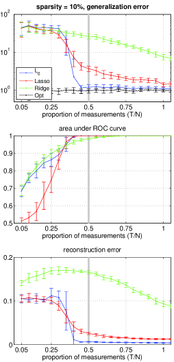
Figure 2: Results for $10\%$ of active customers vs the number of measurements.

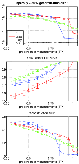
Figure 3: Results for $50\%$ of active customers vs the number of measurements.

In our study of the dependence on $T/N$, we set the noise level to $\beta=1/\sigma^{2}_{P}=1$. As shown in Fig. 2, the generalization errors (top plot) for the three tested methods are similar if the number of samples is small. Once the number of samples reaches certain threshold (in this case $T/N\approx 40\%$) the error of $\ell_{0}$ drops to the error obtained using the actual (optimal) elasticities (denoted by ’Opt’ and black curve), and the decrease in the lasso error is also significant. On the contrary, the performance of ridge regression improves continuously but slowly, remaining worse than what is shown by the other methods. The area under the ROC curve (middle plot) shows that $\ell_{0}$ and ridge methods initially perform similarly and significantly better than lasso. This is consistent with the fact that when the number of samples is small, the lasso outputs a trivial (all zero) solution. However, once the threshold is reached, both lasso and $\ell_{0}$ outperform the ridge method. Finally, the reconstruction error in the sparse case (bottom plot) shows a well pronounced threshold for $\ell_{0}$, which reconstructs the price elasticity pattern perfectly once $\approx 40\%$ or more samples are available. The lasso error, although very small, is not totally reduced, because some coefficients are not set to zero. We observe that the reconstruction error of the ridge method is not monotonic - showing an initial increase and then decrease, which is consistent with the fact that the ridge regression is not optimizing the reconstruction error.

The results are qualitatively different for denser problems, see Fig. 3. Testing the generalization error (top plot), one observes an abrupt transition in both lasso and $\ell_{0}$ methods. However, the transition occurs earlier in the $\ell_{0}$ method ($T/N\approx 80\%$) than in the lasso, which requires $T\approx N$ number of samples to reduce the error significantly. Remarkably, for small $T/N$ (before the threshold) the solution provided by the simplest method (ridge) is the best. The behavior of the area under the ROC curves (middle plot) also differs from the sparse case – the performance of $\ell_{0}$ and lasso below the threshold is not as good as before. Finally, the reconstruction error (bottom plot) is generally worse in this case, and again the ridge method shows the best performace for small $T/N$.

III-B Dependence on the Signal-to-Noise Ratio

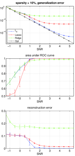
Figure 4: Results for $10\%$ of active customers vs SNR.

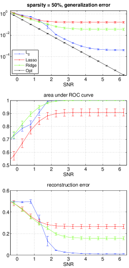
Figure 5: Results for $50\%$ of active customers vs SNR.

We now vary the SNR in a simulated environment of $N=500$ customers. We define the SNR as the log of the average standard deviation of $\vec{\alpha}^{\mathrm{T}}\vec{\rho}(t)$ divided by the standard deviation $\sigma_{P}$. In this case, we choose the number of time steps to be large enough to allow accurate reconstruction for sufficiently large SNR, i.e. $T=250$ samples for a sparsity of $10\%$ and $T=475$ samples for a sparsity of $50\%$. These conditions are shown as gray vertical lines in Figs. 2 and 3, respectively.

Figs. 4 and 5 show that, at sufficiently high SNR, $\ell_{0}$ performs the best. However, when the SNR is low, the other two methods outperform $\ell_{0}$ in all the measures considered, but especially if the problem is dense, see Fig. 5. In the dense case, ridge regression is the best option at low SNR. Note, however, that the bad performance of lasso in the dense case is due to the fact that it requires more samples for denser problems to improve over ridge, see the gray line in Fig. 3.

IV Discussion and Future Work

Our main conclusion is that the sparse reconstruction can be used to extract individual consumer price elasticities from a measured time series of aggregated consumption of real power when this aggregated power is perturbed using small, consumer-specific, random price signal variations. For the reconstruction to be reliable, several conditions must be met: the number of time slots over which consumers do not change their elasticity should be sufficiently large, the proportion of the consumers actually responding should be sufficiently small, and the aggregated consumption is sufficiently large so that the price-driven response is not swamped by the noise of natural fluctuations of consumption. All methods show transitions (smooth or abrupt, and sometimes at different values of the governing parameters) in reconstruction quality. In a regime where the number of samples is insufficient or when the SNR is not sufficiently large, the $\ell_{0}$ method performs worse than the others, and its performance degrades for denser problems. In these bad or marginal cases, one would choose the lasso method over the $\ell_{0}$ method. However, when the unreliable-to-reliable transition has been crossed, the $\ell_{0}$ approach is preferable because it is able to reconstruct the individual price elasticities perfectly, at the cost of more computational time. Further simulations (not discussed in the manuscript) suggest that this phase transition-like behavior becomes sharper with increase in $N$.

The technique described in this manuscript applies practically without modifications to a number of more general settings, for example to account for distributed generation (e.g. from PV systems that include local storage) sold by consumers to the utility. This will require introducing an additional selling-price signal, but it is otherwise identical to the description above. Generalizations accounting for other types of the exogenous signals, e.g. to outside temperature, can also be made as long as they signals are known on a consumer-specific basis.

In a future, we will consider incorporating more details of power systems into the reconstruction, e.g. losses, variation in voltages, and nonlinearity of power flows. Another direction for extensions is more detailed modeling of consumer elasticity that includes the discrete and nonlinear nature of the response [8]. Finally, some of the sparse reconstruction methodology discussed in this manuscript should be useful for analysis of the ”closed loop” distribution markets, e.g. the double auction markets of the Olympic Peninsula Project [5] and several others discussed in recent energy market research [18, 19, 20].

References

- [1] FERC/DOE, “Demand response and advance metering report.” http://www.ferc.gov/legal/staff-reports/11-07-11-demand-response.pdf.
- [2] ENERNOC, “Demand smart.” http://www.enernoc.com/for-businesses/demandsmart.
- [3] ERCOT, “Wind integration reports.” http://www.ercot.com/gridinfo/generation/windintegration/.
- [4] PJM, “Energy market.” http://pjm.com/markets-and-operations/energy.aspx.
- [5] D. Hammerstrom, “Pacific Northwest GridWise (TM) Testbed Demonstration Projects. Part I. Olympic Peninsula Project,” 2007. Technical report, PNNL-17079, Pacific Northwest National Laboratory.
- [6] D. Callaway and I. Hiskens, “Achieving controllability of electric loads,” Proceedings of the IEEE, vol. 99, no. 1, pp. 184–199, 2011.
- [7] K. S. Turitsyn, N. Sinitsyn, S. Backhaus, and M. Chertkov, “Robust broadcast-communication control of electric vehicle charging,” Proceedings of IEEE SmartGridComm 2010, arXiv:1006.0165.
- [8] K. S. Turitsyn, S. Backhaus, M. Ananyev, and M. Chertkov, “Smart finite state devices: A modeling framework for demand response technologies,” Proceedings of CDC 2011, vol. abs/1103.2750, 2011.
- [9] A. E. Hoerl and R. W. Kennard, “Ridge regression: Biased estimation for nonorthogonal problems,” Technometrics, vol. 12, pp. 55–67, 1970.
- [10] I. E. Frank and J. H. Friedman, “A statistical view of some chemometrics regression tools,” Technometrics, vol. 35.
- [11] R. Tibshirani, “Regression shrinkage and selection via the lasso,” Journal of the Royal Statistical Society B, vol. 58, pp. 267–288, 1996.
- [12] N. Meinshausen, “Relaxed lasso,” Computational Statistics & Data Analysis, vol. 52, no. 1, pp. 374–393, 2007.
- [13] H. J. Kappen., “The variational garrote,” 2012, arXiv:1109.0486.
- [14] J. H. Friedman, T. Hastie, and R. Tibshirani, “Regularization paths for generalized linear models via coordinate descent,” Journal of Statistical Software, vol. 33, pp. 1–22, 2 2010.
- [15] L. Breiman, “Better subset regression using the nonnegative garrote,” Technometrics, vol. 37, no. 4, pp. 373–384, 1995.
- [16] E. I. George and R. E. McCulloch, “Variable Selection Via Gibbs Sampling,” Journal of the American Statistical Association, vol. 88, no. 423, pp. 881–889, 1993.
- [17] T. J. Mitchell and J. J. Beauchamp, “Bayesian variable selection in linear regression,” Journal of the American Statistical Association, vol. 83, no. 404, pp. pp. 1023–1032, 1988.
- [18] M. Roozbehani, M. Dahleh, and S. Mitter, “Dynamic pricing and stabilization of supply and demand in modern electric power grids,” Smart Grid Communications (SmartGridComm), pp. 543 – 548, 2010.
- [19] L. Chen, N. Li, L. Jiang, and S. H. Low, “Optimal demand response: problem formulation and deterministic case,” In Control and Optimization Theory for Electric Smart Grids edited by A. Chakrabortty and M. Ilic, Springer, 2012.
- [20] G. Wang, M. Negrete-Pincetic, A. Kowli, E. Shafieepoorfard, S. Meyn, and U. V. Shanbhag, “Real-time prices in an entropic grid,” Conference on Decision and Control, 2011.