Analysis of light scattering off photonic crystal slabs in terms of Feshbach resonances

Abstract

Techniques to deal with Feshbach resonances are applied to describe resonant light scattering off one dimensional photonic crystal slabs. Accurate expressions for scattering amplitudes, free of any fitting parameter, are obtained for isolated as well as overlapping resonances. They relate the resonance properties to the properties of the optical structure and of the incident light. For the most common case of a piecewise constant dielectric function, the calculations can be carried out essentially analytically. After establishing the accuracy of this approach we demonstrate its potential in the analysis of the reflection coefficients for the diverse shapes of overlapping, interacting resonances.

I Introduction

The concept of Feshbach resonances FESH58 has been conceived and applied in the context of quantum mechanical scattering off many-body systems such as nuclei FESH92 atoms or molecules TTHK99 ; CGJT09 . In these systems a Feshbach resonance occurs if the kinetic energy of the incident particle is close to an almost stable intermediate “molecular” state. Elegant techniques to treat Feshbach resonance scattering were developed, cf. Ref. FESH58 , leading to simple and accurate approximation methods. In the present study we propose to extend and apply these techniques to light scattering off photonic crystal slabs. We consider the case of a one dimensional photonic crystal slab – the grating waveguide structure (GWS), cf. Refs. WARO907 ; RSA97 , shown in Fig. 1. The Feshbach resonances are formed by turning a “bound state” (guided mode) into a resonance “state” (barely radiating mode). We will establish the formal connection to Feshbach resonances in quantum systems and, on this basis, we will develop a novel, essentially fully analytical approach to GWS resonances. It is straightforward to generalize this approach to resonance scattering off more complicated, two and three dimensional photonic systems. Its degree of accuracy in these systems however remains to be established.

As for cold atoms where the condition for appearance of Feshbach resonances can be tuned by varying the strength of an external magnetic field, optical systems offer a variety of ways to influence appearance and properties of resonances. By manipulating the parameters of the GWS, qualitative changes of the shape of isolated Feshbach resonances through their Fano interference with non resonant scattering component and, even more interesting, the generation of two or more overlapping resonances can be attained. Apart from the conceptual connection with Feshbach resonances in atomic and nuclear systems our analytic approach carries significant practical value. It establishes easy and intuitively clear relations between the basic photonic crystal slab parameters and the properties of the resonances. It allows systematic studies of various phenomena arising as a result of the resonance interaction. It provides analytic tools to design photonic crystal slabs exhibiting light scattering resonances with desired properties and to understand how to control them.

Guided mode resonances in GWS were studied in Refs.  MP85 , GSST85 and are found in a wide variety of applications, cf. Refs. KLGY10 ; WM93 ; MSJ10 ; BFCBBDKTS10 ; FLPFB10 ; MCWEC08 ; DTZYJF00 ; BLTFS09 ; LTSYM98 ; KYFMHZ05 . In most theoretical investigations of these resonances FMS02 ; FSJ03 ; FAJO02 ; K03 parameter fitting is required for comparison with data or exact numerical calculations MBPK95 ; SSS82 . Recently in Refs. MFK10 ; M09 ; KCLG11 it was recognized that various photonic resonances can be treated as (asymmetric) Fano-Feshbach resonances and their shapes characterized by a fit to the Fano formula. Simple models have been developed, cf. MFK10 ; ZHTH10 which exhibit optical Feshbach or Fano-Feshbach resonances. The majority of the theoretical approaches concentrated on the properties of resonances with TE polarized light. In our formalism a common treatment of TE and TM resonances arises naturally and provides insights into the origin of their different properties.

The central results of our formal development are the expressions (13), (21) for the reflection amplitudes of isolated and the expressions (33), (40) for overlapping TE and TM resonances respectively. Given the dielectric function of the grating waveguide structure and wavelength and angle of the incident light all the quantities appearing in these expressions are analytically calculable. By comparing with the “exact” numerical results we establish the accuracy of our formulation for isolated as well as for overlapping resonances. (For a more detailed presentation of formalism and results cf. EGLL11 .)

It is important to stress that our method is not limited to scattering amplitudes. It actually provides analytic expressions for the entire spatial distributions of the electric and magnetic fields inside and outside the dielectric structure. As an example we use this to analyze the strength of the resonating electric field at the end of Section IV.

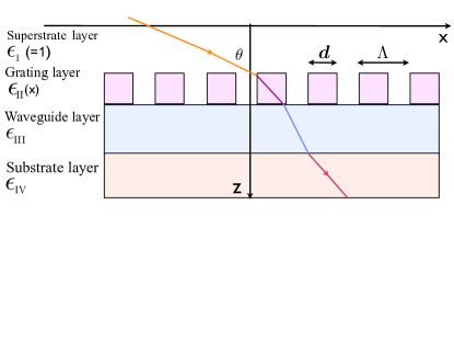
Figure 1: Light incident on a photonic crystal slab with piecewise constant layers with dielectric constants $\epsilon_{I}...\epsilon_{IV}$. Grating period $\Lambda$ and duty cycle $d/\Lambda$ characterize the grating layer (II).

II Isolated resonances

We shall consider the so called “classical” incidence (vanishing y-component of the wavevector) for which TE and TM modes decouple and can be treated separately, cf. Ref. JJWM08 .

In TE polarized waves the electric field is parallel to the grating grooves. In the coordinate system of Fig. 1 its non-vanishing y-component satisfies the wave equation ($c=1$)

$$\Big{(}-\frac{\partial^{2}}{\partial z^{2}}-\frac{\partial^{2}}{\partial x^{2}}-\epsilon(x,z)\omega^{2}\Big{)}E(x,z)=0\,,$$ (1)

with $\omega$ denoting the frequency of the incident light. The non-trivial x-dependence of the dielectric constant is limited to the grating layer and is periodic with grating period $\Lambda$ and corresponding reciprocal lattice vector $K_{g}=2\pi/\Lambda$. Its Fourier components are given by

$$\epsilon_{n}(z)=\frac{1}{\Lambda}\int_{-\Lambda/2}^{\Lambda/2}dx\,\epsilon(x,z)e^{-inK_{g}x}\,.$$

In terms of the Fourier components $E_{n}(z)$ of the electric field the wave equation (1) is converted into a system of ordinary differential equations

$$\sum_{m}D_{nm}E_{m}(z)=0\,,$$ (2)

with

$$D_{nm}=\Big{(}\frac{d^{2}}{dz^{2}}-(k_{x}+nK_{g})^{2}+\omega^{2}\epsilon_{0}(z)\Big{)}\delta_{nm}+\omega^{2}\epsilon_{n-m}(z)(1-\delta_{nm})\,,$$ (3)

and the components of the wave vector $k_{x},\,k_{z}$ of the incident light.

Systems of equations of coupled channels with similar structure are underlying the description of Feshbach resonances in atomic and nuclear physics. A Feshbach resonance occurs if, by neglecting certain couplings, a bound state of the entire system, projectile plus target, exists which when turning on the couplings is converted into a resonance. We proceed here in the same spirit.

In analogy with the distinction between “closed” and “prompt” or “open” channels FESH92 we distinguish here coupled evanescent modes $E_{n}(z)$ which for $z\to\pm\infty$ do satisfy the condition

$$\epsilon_{0}({\pm\infty})\omega^{2}-(k_{x}+nK_{g})^{2}<0\,,$$

and extended modes which do not. To simplify the discussion we focus on the important special case of a “subwavelength grating” where the kinematics is chosen such that the above condition is satisfied only for the $n=0$, extended mode. In terms of the (yet undetermined) evanescent modes, the extended mode is given by

$$E_{0}(z)=E_{0}^{(+)}(z)-\omega^{2}\int dz^{\prime}g_{0}^{E}(z,z^{\prime})\sum_{n\neq 0}\epsilon_{-n}(z^{\prime})E_{n}(z^{\prime})\,,$$ (4)

as is easily verified by applying $D_{00}$ to this equation. Here the electric field $E_{0}^{(+)}$ and the Green’s function $g_{0}^{E}$ solve the homogeneous and the inhomogeneous wave equation respectively

$$D_{00}\,E_{0}^{(+)}=0\,,\quad D_{00}\,g_{0}^{E}(z,z^{\prime})=\delta(z-z^{\prime})\,,$$ (5)

subject to the boundary conditions imposed by the kinematics illustrated in Fig. 1. For $E_{0}^{(+)}$ they are

$$\lim_{z\rightarrow-\infty}E_{0}^{(+)}(z)=e^{ik_{z}z}+r_{0}^{E}e^{-ik_{z}z}\,,\quad\lim_{z\rightarrow\infty}\hskip 2.27626ptE_{0}^{(+)}(z)=t_{0}^{E}e^{i\tilde{k}_{z}z}\,,$$ (6)

with $k_{z},\,\tilde{k}_{z}$ denoting the z-components of the wave vector in the superstrate and substrate layers respectively. The electric field $E_{0}^{(+)}$ accounts for the “background scattering” of light off a dielectric medium with the $x-$averaged $z-$dependent dielectric constant $\epsilon_{0}(z)$. The corresponding (“background”) reflection and transmission amplitudes are denoted by $r_{0}^{E}$ and $t_{0}^{E}$. As is well known MOFS53 , having determined $E_{0}^{+}(z)$ together with it’s partner $E_{0}^{-}(z)$ (wave incident from the substrate), the Green’s function $g_{0}^{E}(z,z^{\prime})$ is given by

$$g_{0}^{E}(z,z^{\prime})=\frac{E_{0}^{+}(z_{>})E_{0}^{-}(z_{<})}{w^{E}}\,,\quad w^{E}=E_{0}^{+}(z)\,dE_{0}^{-}(z)/dz-E_{0}^{-}(z)\,dE_{0}^{+}(z)/dz\,,$$ (7)

with $z_{<,>}$ denoting the smaller and larger of the arguments $z,z^{\prime}$ respectively and $w^{E}$ the $z$-independent Wronskian.

The evanescent modes in (4) can in turn be expressed in terms of $E_{0}(z)$

$$E_{n}(z) = \sum_{m}\int dz^{\prime}\big{(}\tilde{D}^{-1}\big{)}_{nm}(z,z^{\prime})\epsilon_{m}(z^{\prime})E_{0}(z^{\prime})\,,$$ (8)

where

$$\tilde{D}_{nm}=D_{nm}(1-\delta_{n0})(1-\delta_{m0})$$

is the differential operator restricted to the space of evanescent modes.

On the basis of Eqs.(4) and (8) the formal correspondence with quantum mechanical scattering processes in many body systems is established explicitly by the following substitutions (cf. FESH92 )

$$D\to E-H,\;\;\tilde{D}\to Q(E-H)Q,\;\;D_{00}\to P(E-H)P,\,\;\;\epsilon_{n-0}\to-QVP,\quad\epsilon_{0-n}\to-PVQ\,.$$

Here E denotes the total energy and $H=T+V$ is the Hamilton operator of projectile plus target; $P$ and $Q$ are the projection operators on open ($E_{0}$) and closed channels ($\{E_{n},\,n\neq 0\}$) respectively.

Relatives of the quantum mechanical bound states in the closed channels (eigenstates of $QHQ$) are the eigenfunctions of $\tilde{D}$ with vanishing eigenvalues. They are the progenitors of the Feshbach resonances in photonic crystal slabs. Close to the frequency $\omega_{0}$ where one of the eigenvalues $\tilde{\eta}(\omega_{0})=0$ vanishes, $\tilde{D}^{-1}$ is dominated by the corresponding (normalized) eigenmode $\tilde{\mathcal{E}}_{\tilde{\eta}}$ with eigenvalue $\tilde{\eta}(\omega)$ and, as in atomic or nuclear physics applications, can be approximated by

$$\tilde{D}^{-1}(z,z^{\prime})\approx\frac{\tilde{\mathcal{E}}_{\tilde{\eta}}(z)\tilde{\mathcal{E}}_{\tilde{\eta}}(z^{\prime})}{-\tilde{\eta}(\omega)}\,,\quad\int_{-\infty}^{\infty}dz\,\tilde{\mathcal{E}}^{2}_{\tilde{\eta}}(z)=1.$$ (9)

We will refer to this as resonance dominance approximation of an isolated resonance. The coupling of this eigenmode to the extended mode is obtained by expressing the coupled evanescent modes $E_{n}$ in Eq. (4) via Eq.(8) in terms of $E_{0}$ and $\tilde{\mathcal{E}}_{\tilde{\eta}}$. In this way the eigenmode acquires a width and a shift and is turned into an isolated “Feshbach resonance”. This procedure is easily generalized to the case of two or more overlapping resonances where two or more terms in the spectral representation of $\tilde{D}^{-1}$ have to be taken into account.

In scattering of light, by truncating the infinite dimensional space of evanescent modes to one of a large but finite dimension, practically exact results can be obtained in numerical evaluations such as the “RCWA method” MOGA81 or “transfer matrix” techniques MASO08 . With this in mind and in addition to resonance dominance, we also invoke truncation and compute the eigenfunctions $\tilde{\mathcal{E}}_{\tilde{\eta}}$ at the lowest non-trivial level, i.e. , we replace $\tilde{D}$ by its diagonal part

$$\tilde{D}_{nm}\approx D_{nn}\delta_{nm}(1-\delta_{n0})\,.$$

In this “truncation approximation” the exact eigenmodes $\tilde{\mathcal{E}}_{\tilde{\eta}}$ with eigenvalues $\tilde{\eta}(\omega)$ are approximated by the eigenmodes and eigenvalues $\mathcal{E}_{\eta},\eta(\omega)$ of the diagonal elements $D_{nn}$ (cf. Eq. (2)). Since for different $n$ these differ by constants $-(k_{x}+nK_{g})^{2}$ it is sufficient to consider the $n$-independent equation

$$\Big{(}-\frac{d^{2}}{dz^{2}}-\epsilon_{0}(z)\omega^{2}\Big{)}\mathcal{E}_{\eta}(z)=\eta^{E}\,\mathcal{E}_{\eta}(z)\,.$$ (10)

The resonance condition is given by ${\eta}^{E}+(k_{x}+\nu K_{g})^{2}=0$ with an appropriately chosen integer $\nu$. Within resonance dominance and truncation approximation the coupled system of extended and single evanescent modes reads

$$E_{0}(z)=E_{0}^{(+)}(z)-\omega^{2}\int dz^{\prime}g_{0}^{E}(z,z^{\prime})\epsilon_{-\nu}(z^{\prime})E_{\nu}(z^{\prime})\,,\quad E_{\nu}(z)=\frac{\omega^{2}\mathcal{E}_{\eta}(z)}{\eta^{E}+(k_{x}+\nu K_{g})^{2}}\int dz^{\prime}\mathcal{E}_{\eta}(z^{\prime})\epsilon_{\nu}(z^{\prime})E_{0}(z^{\prime}).$$ (11)

The 2nd equation has the form

$$E_{\nu}(z)=\sigma_{\nu}\,\mathcal{E}_{\eta}(z)\,,$$ (12)

with $\sigma_{\nu}$ measuring the degree of excitation of the guided mode. Multiplying the first equation with $\mathcal{E}_{\eta}(z)\epsilon_{\nu}(z)$ and using the relation (12) yields after integrating over $z$ a closed algebraic equation for $\sigma_{\nu}$. Solving this and using the asymptotics of $E^{(+)}_{0}(z)$ (6) and the associated Green’s function (7) one obtains the expression for the total reflection amplitude. We record it for the most common case of piecewise constant index of refraction (Fig. 1) for which the components $\epsilon_{\nu}(z)$ are constants and vanish outside the grating interval for $\nu\neq 0$. We find

$$r^{E}=r_{0}^{E}+\frac{i\sigma_{\nu}\epsilon_{-\nu}{\mathcal{C}}_{+}^{E}}{2k_{z}}=r_{0}^{E}+\frac{i|\epsilon_{\nu}|^{2}\omega^{4}\mathcal{C}^{E\,2}_{+}/2k_{z}}{\eta^{E}+(k_{x}+\nu K_{g})^{2}+|\epsilon_{\nu}|^{2}\omega^{4}\Sigma^{E}}\,,$$ (13)

with the background reflection amplitude $r_{0}^{E}$ (cf. Eq. (6)), the coupling strengths $\mathcal{C}_{\pm}^{E}$ between extended and evanescent modes and the “self - coupling” $\Sigma^{E}$

$$\mathcal{C}_{\pm}^{E}=\int_{I_{g}}dz\mathcal{E}_{\eta}(z)E_{0}^{(\pm)}(z)\,,\quad\Sigma^{E}=\int_{I_{g}}dz\int_{I_{g}}dz^{\prime}\mathcal{E}_{\eta}(z)g^{E}_{0}(z,z^{\prime})\mathcal{E}_{\eta}(z^{\prime})\,.$$ (14)

$\Sigma^{E}$ is generated by transitions from the guided to the extended mode followed by the propagation in the extended mode and the back transition to the evanescent mode. The integrations are carried out over the grating interval ${I_{g}}$. The real part of $\Sigma^{E}$ gives rise to a shift of the resonance position and its imaginary part to the width which accounts for the loss of intensity from the guided to the extended mode. As for the exact solution also in resonance dominance this redistribution of intensity can be shown to preserve flux conservation leading to the standard relation between reflection and transmission coefficients.

The formalism developed so far is easily extended to TM polarized light. The starting point is the wave equation for the y-component of the magnetic field

$$-\Big{(}\partial_{x}\frac{1}{\epsilon(x,z)}\partial_{x}+\partial_{z}\frac{1}{\epsilon(x,z)}\partial_{z}\Big{)}H(x,z)=\omega^{2}H(x,z)\,.$$ (15)

The Fourier transform with respect to the x-coordinate converts this wave equation into the coupled system identical to (2) but for the Fourier components $H_{m}(z)$ of $H(x,z)$ and with the redefined differential operators

$$D_{nm}=-\partial_{z}\gamma_{n-m}(z)\partial_{z}+(k_{x}+nK_{g})(k_{x}+mK_{g})\gamma_{n-m}(z)\,.$$ (16)

The coefficients $\gamma_{n-m}(z)$ denote either the $(n-m)$-th Fourier components of $1/\epsilon(x,z)$ or the inverse of the Toeplitz matrix associated with $\epsilon(x,z)$ (cf. LLI96 ). With this redefinition of $D_{nm}$, the formal development for TE and TM waves becomes identical. We can proceed directly as above applying resonance dominance and truncation approximations and obtaining a coupled system of the extended and resonating evanescent modes (cf. (11))

$$H_{0}(z)=H_{0}^{(+)}(z)+\gamma_{-\nu}\int_{I_{g}}dz^{\prime}g_{0}^{H}(z,z^{\prime})\Theta_{0\nu}H_{\nu}(z^{\prime})\,,\quad H_{\nu}(z)=\frac{\gamma_{\nu}\mathcal{H}_{\nu}(z)}{\omega^{2}-\eta^{H}}\int_{I_{g}}dz^{\prime}\mathcal{H}_{\nu}(z^{\prime})\,\Theta_{\nu 0}H_{0}(z^{\prime})\,.$$ (17)

Here the differential operator

$$\Theta_{nm}=\overleftarrow{\partial_{z}}\;\overrightarrow{\partial_{z}}+(k_{z}+nK_{g})(k_{x}+mK_{g})\,,$$ (18)

and the normalized eigenfunction, the evanescent mode,

$$\Theta_{\nu\nu}\mathcal{H}_{\nu}(z)=\eta^{H}\mathcal{H}_{\nu}(z)\,,\quad\int_{-\infty}^{\infty}dz\,\mathcal{H}^{2}_{\nu}(z)=1,$$ (19)

is chosen such that its eigenvalue $\eta^{H}$ is close to $\omega^{2}$ – the resonance condition in the TM case. The magnetic fields $H_{0}^{\pm}(z)$ and the Green’s function $g_{0}^{H}(z,z^{\prime})$ satisfy the homogeneous and inhomogeneous differential equation (5) respectively with $D_{00}$ given by Eq. (16). The same boundary conditions for $H^{\pm}_{0}(z)$ are imposed as for $E^{\pm}_{0}(z)$ (Eq. (6)).

The Green’s function is given by

$$g_{0}^{H}(z,z^{\prime})=\frac{H_{0}^{+}(z_{>})H_{0}^{-}(z_{<})}{-\gamma_{0}(z)w^{H}(z)}\,,$$ (20)

where $w^{H}(z)$ is the Wronskian given by the same formula as (7) with $E_{0}^{\pm}$ replaced by $H_{0}^{\pm}$. The factor $-\gamma_{0}(z)$ is due to the presence of the first order derivative in the differential operator $D_{00}$ (16). It makes the denominator z-independent as is most easily shown by applying Abel’s formula (cf. KIBO03 ).

The resulting reflection amplitude for the scattering reads

$$r^{H}=r^{H}_{0}-\frac{i\sigma_{\nu}\gamma_{-\nu}\mathcal{C}_{+}^{H}}{2k_{z}}=r^{H}_{0}-\frac{i|\gamma_{\nu}|^{2}\mathcal{C}_{+}^{H\,2}/2k_{z}}{\omega^{2}-\eta^{H}-|\gamma_{\nu}|^{2}\Sigma^{H}}\,.$$ (21)

The strength of the couplings $\mathcal{C}^{H}_{\pm}$ between guided and extended modes and the self coupling $\Sigma^{H}$ are given by

$$\mathcal{C}^{H}_{\pm}=\int_{I_{g}}dz\mathcal{H}_{\nu}(z)\Theta_{\nu 0}H_{0}^{(\pm)}(z)\,,\quad\Sigma^{H}=\int_{I_{g}}dz\int_{I_{g}}dz^{\prime}\mathcal{H}_{\nu}(z)\Theta_{\nu 0}\,g_{0}^{H}(z,z^{\prime})\,\Theta_{0\nu}^{\prime}\mathcal{H}_{\nu}(z^{\prime})\,.$$ (22)

The results (13) and (21) determine the TE and TM reflection amplitudes. As was stressed in the Introduction the quantities entering these expressions are not fitting parameters. They are directly calculable once the properties of the GWS, i.e., the dielectric constants and the sizes of the various layers (cf. Fig.1) as well as the wave vector of the incident light are specified. The eigenvalues $\eta^{E}$ and $\eta^{H}$ and the corresponding eigenfunctions $\mathcal{E}_{\nu}(z)$ and $\mathcal{H}_{\nu}(z)$ (Eqs. (10) and (19)), the functions $E_{0}^{(+)}(z)$ (5) and correspondingly $H_{0}^{(+)}(z)$ together with the corresponding Green’s functions ((7), (20)) are solutions of simple one dimensional equations with piecewise constant coefficients. The background reflection coefficients $r_{0}^{E}$ and $r_{0}^{H}$ are straightforwardly extracted from the asymptotics $z\to-\infty$ of $E_{0}^{(+)}$ and $H_{0}^{(+)}$ respectively. What then remains to be determined are the quantities $\mathcal{C}_{+}^{E,H}$ and $\Sigma^{E,H}$ which are obtained by evaluation of the integrals (14) and (22) respectively. All the necessary calculations which we have outlined can be carried out analytically up to the determination of the eigenvalues $\eta^{E,H}$ – the only quantities which require numerical solution of transcendental algebraic equations.

Let us now ascertain the accuracy of our method. We have chosen typical values for the parameters of the GWS (cf. Fig. 1): the thickness of grating and guided mode layers is 0.1 and 0.4 $\mu$m respectively, the values of $\epsilon$ in the superstrate, the guided mode and the substrate layer are 1, 4, and 2.25 respectively and the values of $\epsilon$ in the grating layer are 1 and 4, the grating period $\Lambda=0.87\,\mu$m and the duty cycle $d/\Lambda=0.5$.

Fig. 2 displays the reflectivity of the $\nu=-1$ TE and TM resonances. It is seen that already to lowest order in the truncation the resonance dominance yields a very good description of both the TE and TM resonances. The somewhat lower accuracy of the TM reflectivity reported also in other approaches (cf. LLI96 and references therein) has its origin in the derivative coupling (the second term in Eq. (15)) between the modes. If applied to the Green’s function $g_{0}^{H}(z,z^{\prime})$ the differential operator $\Theta_{\nu 0}$ (18) generates a $\delta$ function which, in comparison with $\Sigma^{E}$(14), makes the self coupling $\Sigma^{H}$ (22) more important and more sensitive to details of the guided modes.

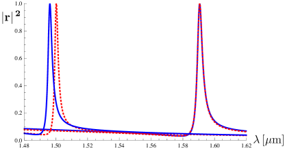
Figure 2: Reflectivities as a function of the wavelength for TM, Eq. (21) (left peak) and TE, Eq. (13) polarized light incident at $5^{\circ}$. Solid line: exact results (obtained by applying transfer matrix techniques MASO08 ), dashed line: results of resonance dominance and truncation approximations.

A phenomenon that has received wide interest in various fields of physics is the Fano interference FANO61 , also termed Fano or Fano-Feshbach resonances (cf. MFK10 and references therein). Its distinct feature is the asymmetric shape of resonance curves. In our context it finds its natural description in terms of interference of isolated Feshbach resonances and the background scattering ($r_{0}^{E,H}$) as indicated by the two terms in the reflection amplitudes in Eqs. (13) and (21). The Feshbach resonance description of Fano interference is closely related to the “temporal coupled-mode formalism” of FSJ03 with the background scattering corresponding to the “direct pathway”. We recall that in our case the background scattering is generated for TE and TM polarizations by the effective dielectric medium defined by $\epsilon_{0}(z)$ and $\gamma_{0}(z)$ respectively. It is negligible with the above choice of the parameters resulting in almost perfect Lorentzian shapes of the isolated resonances in Fig. 2. By changing the value of the period and of the incident angle we can enforce a strong background with a correspondingly strong distortion of the resonance shape as demonstrated in Fig. 3. The level of agreement between exact and approximate calculations confirms the validity of the resonance dominance also in the presence of strong backgrounds.

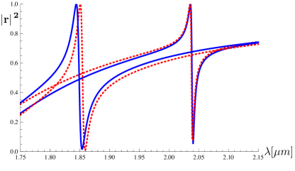
Figure 3: Same as in Fig. 2 with period $\Lambda=0.80\,\mu m$ for angles of the incident light of $85^{\circ}$ (TM) and $70^{\circ}$ (TE).

III Overlapping Feshbach resonances

The formulation of light scattering off GWS in terms of Feshbach resonances is readily generalized to the case of overlapping resonances. For photonic crystal slabs of the structure shown in Fig. 1 overlapping resonances with both TE and TM polarization exist at illumination close to normal incidence independent of the detailed properties of the GWS. For $k_{x}\to 0$ two guided modes are excited, i.e., a resonance with $n=\nu$ is always accompanied by the resonance with $n=-\nu$. We now present an analysis of this class of overlapping resonances. Our treatment is easily generalized to the case of two resonating modes $n=\mu$ and $n=\nu$ with $\mu\neq-\nu$ (cf. EGLL11 ).

Accounting for the additional mode in the resonance dominance approximation (9) leads, after truncation, to the following system of coupled equations for TE waves

$$E_{0}(z) = E_{0}^{(+)}(z)-\omega^{2}\int_{I_{g}}dz^{\prime}g^{E}_{0}(z,z^{\prime})\big{(}\epsilon_{-\nu}E_{\nu}(z^{\prime})+\epsilon_{\nu}E_{-\nu}(z^{\prime})\big{)}\,,$$

$$E_{\pm\nu}(z) = \frac{\omega^{2}}{\eta^{E}+(k_{x}\pm\nu K_{g})^{2}}\,\mathcal{E}_{\eta}(z)\int_{I_{g}}dz^{\prime}\mathcal{E}_{\eta}(z^{\prime})\big{(}\epsilon_{\pm\nu}E_{0}(z^{\prime})+\epsilon_{\pm 2\nu}E_{\pm\nu}(z^{\prime})\big{)}.$$ (23)

In comparison with Eq. (11) this system accounts for the coupling of the extended to two guided modes as well as the interaction between the guided modes. In deriving it we have made use of the property that eigenvalue $\eta^{E}$ and eigenfunction $\mathcal{E}_{\eta}(z)$ (Eq. (10)) are independent of $\nu$. Thus the resonating waves $E_{\pm\nu}(z)$ differ only in their (resonance enhanced) strengths $\sigma_{\pm\nu}$ (cf. Eq. (12)), i. e.,

$$E_{\pm\nu}(z)=\sigma_{\pm\nu}\,\mathcal{E}_{\eta}(z)\,.$$ (24)

Multiplying the first equation of (23) with $\mathcal{E}_{\eta}(z)\epsilon_{\pm\nu}(z)$ and using (24) yields after integrating over $z$ two coupled linear, algebraic equations for the strengths parameters $\sigma_{\pm\nu}$

$$W^{E}\left(\begin{array}[]{ccc}\sigma_{+\nu}\\ \sigma_{-\nu}\\ \end{array}\right)=\omega^{2}\,\mathcal{C}_{+}^{E}\left(\begin{array}[]{ccc}\epsilon_{\nu}\\ \epsilon_{-\nu}\\ \end{array}\right)\,,$$ (25)

with the coupling matrix

$$W^{E}=\left(\begin{array}[]{ccc}\eta^{E}+(k_{x}+\nu K_{g})^{2}+|\epsilon_{\nu}|^{2}\omega^{4}\,\Sigma^{E},&\epsilon_{\nu}^{2}\omega^{4}\,\Sigma^{E}-\epsilon_{2\nu}\omega^{2}\,V^{E}\\ \epsilon_{-\nu}^{2}\omega^{4}\,\Sigma^{E}-\epsilon_{-2\nu}\omega^{2}\,V^{E},&\eta^{E}+(k_{x}-\nu K_{g})^{2}+|\epsilon_{\nu}|^{2}\omega^{4}\,\Sigma^{E}\end{array}\right)\,.$$ (28)

The diagonal elements of $W^{E}$ contain the complex valued self coupling $\Sigma^{E}$ defined in Eq.  (14). In the off-diagonal elements direct couplings $\epsilon_{\pm 2\nu}V^{E}$ between the guided modes appear with

$$V^{E}=\int_{I_{g}}dz\mathcal{E}^{2}_{\eta}(z)\,,$$ (29)

along with the indirect coupling terms $\epsilon_{\pm\nu}^{2}\Sigma^{E}$ via the extended mode. In terms of the matrix elements $W^{E}_{ij}$, the inverse of $W$ is given by

$$(W^{E})^{-1}=\frac{1}{W^{E}_{+}W^{E}_{-}}\left(\begin{array}[]{ccc}W^{E}_{22}&-W^{E}_{12}\\ -W^{E}_{21}&W^{E}_{11}\\ \end{array}\right)\,,$$ (30)

with the eigenvalues of $W^{E}$

$$W^{E}_{\pm}=\eta^{E}+k_{x}^{2}+\nu^{2}K_{g}^{2}+\big{|}\epsilon_{\nu}\big{|}^{2}\omega^{4}\,\Sigma^{E}\pm\Big{[}(2k_{x}\nu K_{g})^{2}+\omega^{4}$$

$$\,\cdot\Big{(}\big{(}|\epsilon_{\nu}|^{2}\omega^{2}\,\Sigma^{E}-|\epsilon_{2\nu}|\cos\varphi^{E}V^{E}\big{)}^{2}+|\epsilon_{2\nu}|^{2}\sin^{2}\varphi^{E}\,V^{E\,2}\Big{)}\Big{]}^{1/2}.$$

(31)

We have introduced the relative phase between $\epsilon_{2\nu}$ and $\epsilon_{\nu}^{2}$

$$e^{i\varphi^{E}}=\frac{\epsilon_{2\nu}\epsilon_{\nu}^{\star\,2}}{|\epsilon_{2\nu}\epsilon_{\nu}^{2}|}\,,$$ (32)

which will be seen to distinguish different types of interacting resonances. The phase $\varphi^{E}$ appears as a result of the interference of the 2-step process via the extended mode and the one step process connecting directly the two guided modes. The combination of the strengths $\sigma_{\pm\nu}$ which determines the reflection amplitude is easily calculated

$$r^{E} = r^{E}_{0}+\frac{i}{2k_{z}}\big{(}\sigma_{\nu}\,\epsilon_{-\nu}+\sigma_{-\nu}\,\epsilon_{\nu}\big{)}\omega^{2}\mathcal{C}^{E}_{+}=r^{E}_{0}+\frac{i|\epsilon_{\nu}|^{2}\omega^{4}\mathcal{C}^{E\,2}_{+}W^{E}_{0}}{k_{z}W^{E}_{+}W^{E}_{-}},$$

$$W^{E}_{0} = \eta^{E}+k_{x}^{2}+\nu^{2}K_{g}^{2}+|\epsilon_{2\nu}|\cos\varphi^{E}\,\omega^{2}V^{E}\,.$$ (33)

The same procedure applies to the formulation of overlapping TM polarized Feshbach resonances. In order to keep the presentation transparent we restrict it to the limit of small $|k_{x}|$ where the interaction of the resonances is significant and where the two guided modes

$$\mathcal{H}_{\eta}(z)=\mathcal{H}_{\nu}(z)\approx\mathcal{H}_{-\nu}(z)\,,$$ (34)

can be identified. (The numerical results to be discussed later have been obtained without resorting to this approximation.) In this limit we obtain the following system of coupled equations for the two evanescent components $H_{\pm\nu}(z)$ and the extended mode $H_{0}(z)$

$$H_{0}(z) = H_{0}^{(+)}(z)+\int_{I_{g}}dz^{\prime}g^{H}(z,z^{\prime})\left(\gamma_{-\nu}\Theta_{0,\nu}H_{\nu}(z^{\prime})+\gamma_{\nu}\Theta_{0,-\nu}H_{-\nu}(z^{\prime})\right),$$

$$H_{\pm\nu}(z) = \frac{1}{\omega^{2}-\eta^{H}}\mathcal{H}_{\eta}(z)\int_{I_{g}}dz^{\prime}\mathcal{H}_{\eta}(z^{\prime})\left(\gamma_{\pm\nu}\Theta_{\pm\nu,0}H_{0}(z^{\prime})+\gamma_{\pm 2\nu}\Theta_{\pm\nu,\mp\nu}H_{\mp\nu}(z^{\prime})\right)\,,$$ (35)

which is of the same structure as the one for TE polarization and is solved in the same way. We introduce the matrix ($W^{H}$) connecting the strength parameters and the Fourier coefficients of the (inverse) dielectric constant of the grating layer

$$W^{H}\left(\begin{array}[]{ccc}\sigma_{+\nu}\\ \sigma_{-\nu}\\ \end{array}\right)=\mathcal{C}_{+}^{H}\left(\begin{array}[]{ccc}\gamma_{\nu}\\ \gamma_{-\nu}\\ \end{array}\right)\,.$$ (36)

Comparing the systems (23) and (35) the matrix elements and the eigenvalues of $W^{H}$ can be read off from Eqs. (28) and (31)

$$W^{H}_{\pm}=\omega^{2}-\eta^{H}-|\gamma_{\nu}|^{2}\Sigma^{H}\mp\Big{[}(2\zeta k_{x}\nu K_{g})^{2}+\left(|\gamma_{\nu}|^{2}\Sigma^{H}+|\gamma_{2\nu}|\cos{\varphi^{H}}V^{H}\right)^{2}+|\gamma_{2\nu}|^{2}\sin^{2}{\varphi^{H}}V^{H\,2}\Big{]}^{1/2}.$$

(37)

For TM polarization, the direct coupling via $\gamma_{\pm 2\nu}$ between the two guided modes is given by

$$V^{H}=\int_{I_{g}}dz\,\mathcal{H}_{\eta}(z)\Theta_{\nu,-\nu}\mathcal{H}_{\eta}(z)\,.$$ (38)

and the relative phase by

$$e^{i\varphi^{H}}=\frac{\gamma_{2\nu}\gamma_{\nu}^{\star\,2}}{|\gamma_{2\nu}\gamma_{\nu}^{2}|}\,.$$ (39)

Furthermore, to lowest order, we have taken into account the change of the eigenvalues $\eta^{H}$ for small $k_{x}$

$$\Delta\eta^{H}_{\pm\nu}=\pm 2\zeta\nu K_{g}k_{x},\;\;\;\zeta=\int_{-\infty}^{\infty}dz\gamma_{0}(z)\mathcal{H}^{2}_{\eta}(z)\,.$$

The structure of the reflection amplitude for TM polarization

$$r^{H}=r_{0}^{H}-\frac{i|\gamma_{\nu}|^{2}\mathcal{C}_{+}^{H\,2}W^{H}_{0}}{k_{z}W^{H}_{+}W^{H}_{-}}\,,\quad W^{H}_{0}=\omega^{2}-\eta^{H}+|\gamma_{2\nu}|\cos\varphi^{H}V^{H}\,,$$ (40)

is the same as that for TE polarization (33).

As for isolated resonances our treatment of overlapping resonances has led us to a well defined algorithm for the computation of the reflection coefficient which does not contain any adjustable parameter. The only new quantities appearing here are the direct interactions $V$ (Eqs. (29) and (38)) which again can be evaluated analytically in closed form.

IV Patterns of Interactions of Overlapping Resonances

Eqs. (33) and (40) provide a full solution for the overlapping resonance case. The analytic nature of these expressions allows a detailed analysis of various patterns arising as the overlapping resonances affect each other. We start by observing that, as expected and independent of the details, the single resonance result (13) is reached in the limit where, for TE polarization, the square root in Eq. (31) is dominated by the term $\sim|k_{x}\nu K_{g}|$

$$\frac{W^{E}_{0}}{W^{E}_{+}W^{E}_{-}}\hskip 5.69046pt\longrightarrow_{{}_{\large{|k_{x}|\to\infty}}} \sum_{\mu=\pm\nu}\frac{1}{2}\frac{1}{\eta^{E}+(k_{x}+\mu K_{g})^{2}+|\epsilon_{\mu}|^{2}\omega^{4}\Sigma^{E}}.$$

This limit can also be shown to be satisfied for TM polarized resonances provided the approximation (34) is not invoked.

With decreasing $k_{x}$ the coupling between the resonances sets in and modifies their properties. Independent of the strength of this coupling are the averages of positions and widths of the resonances

$$\frac{W^{E}_{+}+W^{E}_{-}}{2}=\eta^{E}+k_{x}^{2}+\nu^{2}K_{g}^{2}+\big{|}\epsilon_{\nu}\big{|}^{2}\omega^{4}\,\Sigma^{E}\,,\quad\frac{W^{H}_{+}+W^{H}_{-}}{2}=\omega^{2}-\eta^{H}-|\gamma_{\nu}|^{2}\Sigma^{H}\,.$$

They coincide with the averages of the denominators of the reflection coefficients (13) and (21) for the isolated resonances with the indices $\pm\nu$. Thus broadening of one of the resonances is accompanied by narrowing of the other. This is reminiscent of motional narrowing BlPP48 or of super- D54 and subradiance PCPCL85 for coupled emitters.

The coupling of the resonances increases or decreases their distance $\big{|}\mbox{Re}(W_{+}-W_{-})\big{|}$ depending on the structure of the GWS. As our results show, the change in the distance depends on the interplay between strengths and phase of the self coupling $\Sigma$ and the direct coupling $V$. Obviously, for sufficiently large values of the direct coupling terms $|\epsilon_{2\nu}V^{E}|,|\gamma_{2\nu}V^{H}|$ one will find a repulsion of the resonances. We will discuss an example of such a case below. It is remarkable that the system of overlapping resonances can be tuned to exhibit either “level” repulsion or attraction by variation of an external parameter - the wave vector component $k_{x}$ of the incoming light.

A peculiarity of the interacting resonances is the appearance of a zero in the resonance amplitude, i.e. when

$$W_{0}(\omega,k_{x})=0,$$

in Eq. (33). The presence of this zero may distort significantly the shape of the reflectivity a phenomenon reminiscent of Fano resonances. Indeed the expressions (33) and (40) for the reflection amplitudes have the structure of a product of a Lorentzian and of a Fano resonance. The appearance of this zero can also be interpreted as a result of a cancellation between the contributions from the eigenstates of $W^{E,H}$ (cf. Eqs. (25), (36)). This destructive interference causes a transparency window within the resonance and is therefore closely related to the “EIT” phenomenon (electromagnetically induced transparency), (cf. Refs. H97  ,FLIM05 ).

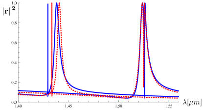
Figure 4: Reflectivity for overlapping resonances as a function of the wavelength for TM (left peaks, cf. Eq. (40)) and TE (Eq. (33)) polarized light incident at $0.05^{\circ}$ with 50% duty cycle. Solid lines: exact results obtained by applying transfer matrix techniques, Ref. MASO08 . Dashed lines: results of resonance dominance and truncation approximations.

The limit of small $k_{x}$ offers further analytical insights into the relation between the dynamics and the structure of the interacting resonances. We consider first the case

$$\sin\varphi^{E,H}V^{E,H}=0.$$ (41)

As a function of the wavelength of the incident light the reflection coefficients for TE and TM polarizations exhibit a single resonance for vanishing $k_{x}$ (cf. Eqs. (31), (37)). Its width is twice as large as that of an isolated resonance (cf. Eqs.(13) and (21)). In approaching the $k_{x}=0$ limit the widths of one of the coupled resonances approaches zero. A singularity is prevented by the presence of the factor $W_{0}$ which, in this limit also approaches zero. In order to understand the transition from the single resonance at $k_{x}=0$ to two interacting resonances at finite but small $k_{x}$ we write $W_{\pm}^{E}$ as

$$W_{+}^{E}=W_{0}^{E}(k_{x})+2(|\epsilon_{\nu}|^{2}\omega^{4}\Sigma^{E}-|\epsilon_{2\nu}|\cos\varphi^{E}V^{E})+\delta W^{E},$$

$$W_{-}^{E}=W_{0}^{E}(k_{x})-\delta W^{E},$$

$$\delta W^{E}=\frac{2(k_{x}\nu K_{g})^{2}}{|\epsilon_{\nu}|^{2}\omega^{4}\Sigma^{E}-|\epsilon_{2\nu}|\cos\varphi^{E}V^{E}}\,.$$ (42)

For $k_{x}\neq 0$, the zero of $W_{0}$ in the numerator is no longer canceled by the zero of $W_{-}$ which is shifted into the complex plane. At small but finite $k_{x}$ a narrow resonance is present together with the zero of the numerator. The properties of the “broad” resonance ($W_{+}$) are only weekly affected. Whether or not the narrow resonance and the zero of $W_{0}$ overlap with the broad resonance, i.e., the size of the bandgap, depends on the shift $2(|\epsilon_{\nu}|^{2}\omega^{4}\mbox{Re}\Sigma^{E}-|\epsilon_{2\nu}|\cos\varphi^{E}V^{E})$ which in turn is sensitive to the duty cycle. In the limit considered the ratio $W_{0}^{E}/W_{-}^{E}$ generates a Fano resonance and $1/W_{+}$ a Lorentzian. Indeed expanding $W_{-}^{E}$ in the frequency around the zero of its real part yields the standard expression for Fano resonances MFK10 . The asymmetry (Fano-) parameter is given by $q=\cot\alpha$ with $\alpha$ denoting the phase of $|\epsilon_{\nu}|^{2}\omega^{4}\Sigma^{E}-|\epsilon_{2\nu}|\cos\varphi^{E}V^{E}$.

The same analysis can be carried out for overlapping resonances with TM polarization. The shape of two TE and TM overlapping resonances calculated exactly and in resonance dominance approximation are shown in Fig. 4. The results confirm our analysis. The coincidence of the narrow and wide resonances for TE polarization is due to the dominance of the imaginary part of the self coupling $\Sigma^{E}$ (14) in the expression for $\delta W^{E}$ (42) while their separation for TM polarization is a result of the dominance of the real part of $\Sigma^{H}$ (22).

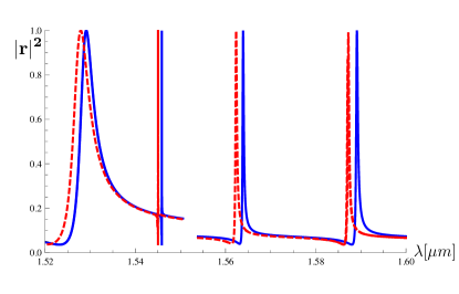
Figure 5: Reflectivity for TE polarization as a function of the wavelength. Solid lines: exact values, dashed lines: resonance dominance approximation. Left: The same structure and parameters as in Fig. 4 but with $75\%$ duty cycle. Right: $\theta=0.005^{\circ}$, with the grating structure (44) and the parameters (45). The curves have been shifted to the right by 50 nm.

Expression (42) for $\delta W^{E}$ indicates that the coincidence between the two resonances for TE polarization does not occur and the non vanishing gap between the resonances is generated when the direct coupling term $\epsilon_{2\nu}\,V^{E}$, Eq. (29), is present. For symmetry reasons, the Fourier component $\epsilon_{2\nu}$ vanishes for 50% duty cycle. The left part of Fig. 5 displays the importance of the direct coupling term at 75% duty cycle. A band gap about 4 times as large as the width of the broad resonance is generated. Practically not affected by this term is the ratio of about 500 between the broad and the narrow resonances.

A more balanced distribution of the widths can be achieved if the condition complementary to (41) is realized for which the direct resonance coupling dominates the self coupling.

$$\varphi^{E,H}=\pm\frac{\pi}{2}\,,\quad\frac{|\epsilon_{\nu}^{2}|\omega^{2}|\Sigma^{E}|}{|\epsilon_{2\nu}|V^{E}}\ll 1\,.$$ (43)

In this limit we find (cf. Eq. (31)) for sufficiently small $k_{x}$

$$W_{\pm}^{E}=\eta^{E}+k_{x}^{2}+\nu^{2}K_{g}^{2}+\big{|}\epsilon_{\nu}\big{|}^{2}\omega^{4}\,\Sigma^{E}\pm\Big{[}\omega^{2}|\epsilon_{2\nu}|V^{E}+\frac{|\epsilon_{\nu}|^{4}\omega^{8}\Sigma^{E\,2}+4k_{x}^{2}\nu^{2}K_{g}^{2}}{2\omega^{2}|\epsilon_{2\nu}|V^{E}}\Big{]}\,.$$

The resulting form is quite different from what we have encountered so far. The direct interaction $V^{E}$ generates repulsion between the two resonances which guarantees that the gap between the resonances does not vanish. The resonances do not overlap and their widths are equal and coincide with that of an isolated resonance. Realization of this limit can not be achieved in simple binary gratings such as the one shown in Fig. 1. Let us instead consider the following more complicated structure

$$\epsilon(x)=\theta(\Lambda^{2}-4x^{2})\Big{[}\epsilon_{\mbox{min}}+\delta\epsilon\,\big{(}\theta(-d-x)+\theta(x-d)\big{)}\Big{]},$$ (44)

with the parameters

$$\Lambda=0.87\,\mu m,\;\;d/\Lambda=0.2,\;\;\epsilon_{\mbox{min}}=1,\;\;\delta\epsilon=3\,.$$ (45)

The corresponding results are shown in the right part of Fig. 5 indicating that the desired limit is indeed realized in this structure and confirming our analytical insights.

Besides the reflection and transmission coefficients, our approach provides expressions for the field strengths in particular in and close to the waveguide layer (Fig. 1). For isolated resonances, the strengths $\sigma_{\nu}$ of the evanescent modes $E_{\nu}(z),H_{\nu}(z)$ are up to a non-resonating factor (cf. Eq. (13)) given by the resonating part $r^{E,H}-r_{0}^{E,H}$ of the corresponding reflection coefficient. For overlapping resonances a new resonating contribution to the field strengths arises. Using the equations (24-31) we evaluate the evanescent electric field with the result

$$E_{\nu}(x,z) = \big{(}E_{\nu}(z)e^{i\nu K_{g}x}+E_{-\nu}(z)e^{-i\nu K_{g}x}\big{)}e^{ik_{x}x}$$

$$= \frac{2\epsilon_{\nu}\omega^{2}C_{+}^{E}e^{ik_{x}x}}{W^{E}_{+}W^{E}_{-}}\Big{\{}W_{0}\cos\nu K_{g}x+\big{(}2ik_{x}\nu K_{g}+|\epsilon_{2\nu}|\omega^{2}\sin\varphi^{E}V^{E}\big{)}\sin\nu K_{g}x\Big{\}}\,\mathcal{E}_{\eta}(z)\,.$$

As for isolated resonances, the first term is proportional to $r^{E}-r_{0}^{E}$, while the second term, due to the absence of $W_{0}$ in the numerator develops a singular point in the $\theta-\omega$ plane of the type

$$E_{\nu}(x,z)\sim\frac{\theta\tilde{\Sigma}}{\omega-\omega_{0}+\theta^{2}\tilde{\Sigma}}\;,$$

where $\tilde{\Sigma}$ is a complex constant. In a lossless medium, at the frequency $\omega_{0}$ where $W_{0}^{E}$ vanishes, the evanescent contribution to the field diverges with vanishing angle of incidence $\theta$.

V Conclusion

We have shown that resonances in light scattering off one dimensional photonic crystal slabs are, in a precise sense, Feshbach resonances. This allowed us to developed a novel, accurate and essentially analytic approximation scheme. As demonstrated in the analysis of the intricate patterns of interacting resonances the advantage of our approach in comparison with various types of parametrization and exact numerical simulations resides in the explicit connection between important quantities like the reflection coefficient and the structure of the GWS. This approach should be useful for the design of photonic crystal slabs with given requirements on reflection or transmission coefficient or on strength and phases of electric and magnetic fields. It can be extended to the analysis of several overlapping resonances or to GWS built of layers of metamaterials, cf. LZMH10 . The extension to two and three dimensional photonic systems appears to be feasible as well. F.L. is grateful for the support and the hospitality at the Department of Condensed Matter, Weizmann Institute. This work is supported in part by the Albert Einstein Minerva Center for Theoretical Physics and by a grant from the Israeli Ministry of Science.

References

- (1) H. Feshbach, Ann. of Phys. 5, (1958), 357, Ann. of Phys. 19, (1962) 287.
- (2) H. Feshbach, Theoretical Nuclear Physics, Nuclear Reactions, (John Wiley & Sons, New York, 1992)
- (3) E. Timmermans, P. Tommasini, M. Hussein, A. Kerman, Phys. Rep. 315, (1999), 199.
- (4) C. Chin, R. Grimm, P. Julienne and E. Tiesinga, Rev. Mod. Phys. 82, (2010), 1225.
- (5) S. S. Wang, R. Magnusson, J.S. Bagby, M. G.Moharam, J. Opt. Soc. Am. A 7, (1990), 1470.
- (6) D. Rosenblatt, A. Sharon, and A. A. Friesem, IEEE J. Quant. Electron. 33, (1997) 2038.
- (7) L. Mashev and E. Popov, Optics Comm. 55, (1985), 377.
- (8) G. A. Golubenko, A. S. Svakhin, V. A. Sychugov, and A. V. Tishchenko, Sov. J. Quantum Electron. 15, (1985) 886.
- (9) O. Katz, J. M. Levitt, E. Grinvald, and Y. Silberberg, Opt. Express 18, (2010), 22693.
- (10) S. S. Wang and R. Magnusson, Appl. Opt. 32, (1993), 2606.
- (11) R. Magnusson, M. Shokooh-Saremi, and E. G. Johnson, Opt. Lett. 35, (2010) 2472.
- (12) F. Brückner, D. Friedrich, T. Clausnitzer, M. Britzger, O. Burmeister, K. Danzmann, E. Kley, A. Tünnermann, and R. Schnabel, Phys. Rev. Lett. 104, (2010), 163903.
- (13) D. Fattal, J. Li, Z. Peng, M. Fiorentino, and R. G. Beausoleil, Nature Photon. 4, (2010), 466.
- (14) M. Lu, S. S. Choi, C. J. Wagner, J. G. Eden, and B. T. Cunningham, Appl. Phys. Lett. 92, (2008), 261502.
- (15) A. Donval, J. Toussaere, E. Zyss, G. Levy-Yurista,E. Jonsson, and A.A Friesem, Synthetic Metals 124, (2001), 19.
- (16) O. Boyko, F. Lemarchand, A. Talneau, A.-L. Fehrembach, and A. Sentenac, J. Opt. Soc. Am. A 26, (2009), 676.
- (17) Z. S. Liu, S. Tibuleac, D. Shin, P. P. Young, and R. Magnusson, Opt. Lett. 23, (1998), 1556.
- (18) T. Katchalski, G. Levy-Yurista, A. A. Friesem, G. Martin, R. Hierle, and J. Zyss, Opt. Express 13, (2005), 4645.
- (19) A.-L. Fehrembach, D. Maystre, and A. Sentenac, J. Opt. Soc. Am. A 19, (2002), 1136.
- (20) S. Fan, W. Suh, and J. D. Joannopoulos, J. Opt. Soc. Am. A, 20, (2003), 569.
- (21) S. Fan, J. D. Joannopoulos, Phys. Rev.B 65, (2002), 235112.
- (22) K. Koshino, Phys. Rev. B 67, (2003), 165213.
- (23) M. G. Moharam, D. A. Pommet, E. B. Grann, T. K. Gaylord, J. Opt. Soc. Am. A 12, (1995), 1077.
- (24) P. Sheng, R. S. Stepleman and P. N. Sanda, Phys. Rev. B 26, (1982), 2907.
- (25) A. E. Miroshnichenko, S. Flach, and Y. S. Kivshar, Rev. Mod. Phys. 82, (2010), 2257.
- (26) A. E. Miroshnichenko, Phys. Rev. E 79, (2009), 026611.
- (27) Ming Kang, Hai-Xu Cui, Yongnan Li, Bing Gu, Jing Chen and Hui-Tian Wang J. Appl. Phys. 109, (2011), 014901.
- (28) XU DaZhi, LAN Hou, SHI Tao, DONG Hui and SUN ChangPu, Science China 53, (2010), 1234.
- (29) I. Evenor, E. Grinvald, F. Lenz, S. Levit, arXiv:1111.0208
- (30) J. D. Joannopoulos, S. G. Johnson, J. N. Winn and R. D. Meade, Photonic Crystals Molding the Flow of Light (Princeton University Press, Princeton and Oxford, 2008)
- (31) M. G. Moharam and T. K. Gaylord, J. Opt. Soc. Am. 71, (1981), 811.
- (32) P. Markoš, C. M. Soukoulis, Wave Propagation, (Princeton University Press, Princeton and Oxford, 2008)
- (33) P. M. Morse and H. Feshbach, Methods of Theoretical Physics Vol. 1, (McGraw-Hill, New York, 1953)
- (34) L. Li, J. Opt. Soc. Am. A 13, (1996), 1870.
- (35) A. C. King, J. Billingham and S. R. Otto, Differential Equations, (Cambridge University Press, Cambridge, 2003)
- (36) U. Fano, Phys. Rev. 124, (1961), 1866.
- (37) N. Bloembergen, E. M. Purcell, and R. V. Pound, Phys. Rev. 73, (1948), 679.
- (38) R. H. Dicke, Phys. Rev. 93, (1954), 99.
- (39) D. Pavolini, A. Crubellier, P. Pillet, L. Cabaret, and S. Liberman, Phys. Rev. Lett. 54, (1985), 1917.
- (40) S. E. Harris, Physics Today 50, 36, (1997)
- (41) M. Fleischhauer, A. Imamoglu, J. P. Marangos, Rev. Mod. Phys. 77, (2005), 633.
- (42) B. Lukyanchuk, N. I. Zheludev, S. A. Maier, N. J. Halas, P. Nordlander, H. Giessen, and C. T. Chong, Nat. Mater. 9, (2010), 707.