A new method for measuring the absolute neutrino mass

Abstract

The probability of the event that a neutrino produced in pion decay is detected in the intermediate $T$ shorter than the life-time $\tau_{\pi}$, $T\leq\tau_{\pi}$, is sensitive to the absolute mass of the neutrino. With a newly formulated S-matrix $S[T]$ that satisfies the boundary conditions of the experiments at a finite $T$, the rate of the event is computed as $\Gamma_{0}+\tilde{g}(\omega_{\nu},{T};\tau_{\pi})\tilde{\Gamma}_{1}$, where $\tilde{g}(\omega_{\nu},{T};\tau_{\pi})$ depends weakly on $\tau_{\pi}$ and $\omega_{\nu}={m_{\nu}^{2}c^{4}}/{(2E_{\nu}\hbar)}$, $c$ is the speed of light. $\Gamma_{0}$ is the standard one and the correction, $\tilde{g}(\omega_{\nu},{T};\tau_{\pi})\tilde{\Gamma}_{1}$, reflects relativistic invariance and is rigorously computed via the light-cone singularity of the system and reveals the diffraction pattern of a single quantum. The formula explains unsolved anomalies of neutrino experiments and indicates the heavy neutrino mass, $0.098\pm 0.022$ or $0.083\pm 0.026$ eV/ $c^{2}$ for normal or inverted mass hierarchies, respectively.

1 Neutrino interference

The probability of the event that a particle produced in a decay or scattering is detected at a finite time-interval $T$ was known to deviate from that of Fermi’s golden rule [1]. It was found recently [2] that the probability has a constant term in addition to a $T$-linear term,

$$P=\Gamma_{0}T+P^{(d)},$$ (1)

where $\Gamma_{0}$ is the known rate and $P^{(d)}$ is constant. $P^{(d)}$ has an origin in kinetic-energy non-conserving term at a finite $T$, and a new energy scale, ${m^{2}c^{4}\over E}$, where $m$ and $E$ are the mass and energy of the detected particle. $P^{(d)}$ is proportional to a size of the particle’s wave function, and is smaller than $\Gamma_{0}T$ in many situations and has been ignored. As regards its relevance with physical phenomena, $P^{(d)}$’s magnitude is a key. This term is necessary in the processes of $\Gamma_{0}=(\approx)0$, or small $T$. There are two cases in the former,

$$\Gamma_{0}=0,\ P^{(d)}=0,$$ (2)

$$\Gamma_{0}=(\approx)0,\ P^{(d)}\neq 0.$$ (3)

Equation $(\ref{case1})$ corresponds to a process forbidden by an exact symmetry such as charge conservation, and Equation $(\ref{case2})$ corresponds to a process forbidden by the conservation-law of kinetic energy. Equation $(\ref{case1})$ is a trivial case, but Equation $(\ref{case2})$ is a non-trivial case. $P^{(d)}$ must be included for the study of the process connected with this transiton. We study an example of Eq. $(\ref{case2})$ that involves light particles.

Neutrinos produced in pion decay reveal large finite-size corrections [2]. Neutrino physics in this region has been less explored and all previous experiments are not in-consistent with the presence of $P^{(d)}$ within experimental uncertainties [3]. In the asymptotic region, flavor oscillations have been observed and made to determine the mass-squared difference and other parameters possible. The present paper shows that the probability of the event that the neutrino is detected at $T\leq\tau_{\pi}$, where $\tau_{\pi}$ is the pion’s life-time, is observable and supplies the information on the neutrino mass. A new experimental method for determining the absolute neutrino mass is presented.

In the present region, kinetic energy of the daughters is not constant, due to finite interaction energy. Thus the state becomes non-uniform in time and reveals an interference. The variation of kinetic energy, $\Delta E$, is extremely small of the order of $G_{F}^{2}$, where $G_{F}$ is the Fermi coupling constant, and causes the interference pattern to the amplitude and probability in $T\leq{\hbar\over\Delta E}$. The pattern formed in the amplitude in a microscopic region initially is transmitted to large region, because a group of neutrino waves have almost the same phase and group velocity $\vec{v}$ and can move in parallel for a certain period, $\delta t$, with relative phases kept constant. Thus the pattern appears even at a macroscopic distance much larger than de Broglie wave length. Photon, neutrino, and other light particles or waves show this macroscopic quantum effect. The neutrino in the leptonic or semi-leptonic decays such as $\pi(K)\rightarrow lepton+\nu$ or $K\to\pi+lepton+\nu$ shows this phenomenon but the massive particles such as the charged leptons in the above processes or mesons in the non-leptonic decays such as $K^{\pm}\rightarrow\pi^{\pm}+\pi^{0}$ do not.

To compute $P^{(d)}$ involves the consideration of boundary conditions. The transition rates at $T$ were computed before with $S[\infty]$ which satisfies the boundary condition at $T=\infty$, and did not show clear $T$-dependence [5, 6, 4, 7, 8, 9, 10]. Now, the probability of the event that the particle is detected at $T$ must be computed with the amplitude which satisfies the boundary conditions at $T$. The correct amplitude is not represented with $S[\infty]$. To compute the probability of the experiments at the $T\leq\tau_{\pi}$ [4], the S-matrix, $S[T]$, defined by wave functions of the initial and final states at $T$, which satisfies the boundary conditions at $T$, was formulated in Ref. [2]. The deviations of the rates from those obtained by Fermi’s golden rule were found by using $S[T]$ [2]. They are large for the neutrinos and small for the charged leptons. The corrections depend on the boundary conditions at $T$, and have the form of $1/{T}$ of universal properties determined by the parameters of Lagrangian. They become significant in forbidden processes of light particles in which the rate $\Gamma_{0}$ vanishes, and are detectable in experiments of an energy resolution of much larger than $\Delta E$ but of the order of $(G_{F})^{0}$.

We study the probability in detail and show that the finite-size correction to the probability that depends on the absolute neutrino masses emerges at a macroscopic ${T}$. Because neutrinos interact extremely weakly with matter and are not disturbed by environment, the effects are easily observed. The detailed analysis of the neutrino spectrum and its implications to the neutrino mass are presented.

Comparing the neutrino spectrum with previous experiments at $T\leq\tau_{\pi}$, we find an indication of the heavy neutrino mass, $0.083\pm 0.026$ for inverted or $0.098\pm 0.022$ $\text{eV}/c^{2}$ for normal mass hierarchies, from its comparison with LSND.

2 Wave function of pion and daughters and $S[T]$

$S[T]$ is determined from the wave functions of the in-coming and out-going waves at $T$ in the system described with a Lagrangian density composed of a field of pion, $\varphi_{\pi}(x)$, of charged lepton, $l(x)$, and of neutrino, $\nu(x)$. That has a four-Fermion coupling

$$\mathscr{L}=\mathscr{L}_{0}+\mathscr{L}_{\text{int}},$$ (4)

$$\mathscr{L}_{0}={\partial_{\mu}}\varphi_{\pi}^{*}{\partial^{\mu}}\varphi_{\pi}-m_{\pi}^{2}\varphi_{\pi}^{*}\varphi_{\pi}+\bar{l}(\ooalign{\hfil/\hfil\crcr$p$}-m_{l})l+\bar{\nu}(\ooalign{\hfil/\hfil\crcr$p$}-m_{\nu})\nu,$$ (9)

$$\mathscr{L}_{int}=gJ_{\text{hadron}}^{V-A}\times J_{\text{lepton}}^{V-A}+\mathscr{L}_{\text{counter}},\ g=G_{F}/{\sqrt{2}},$$

where $J_{i}^{V-A}$ is $V-A$ current, and $\mathscr{L}_{\text{counter}}$ is a counter term of pion field. In this paper $\mathscr{L}_{\text{counter}}=\delta\omega_{0}\varphi_{\pi}^{*}\varphi_{\pi}$ is applied. Majority of the results are obtained from the lowest order terms in perturbative expansions, and are the same in electro-weak gauge theory. The case without the flavor mixing is studied first for clarifying the essence easily. Due to Poincare invariance, momenta of the fields can be any value from $-\infty$ to $+\infty$.

2.1 Wave function

$|\Psi(t)\rangle$ of the pion and decay products satisfies the Schrödinger equation,

$$i\hbar{\partial\over\partial t}|\Psi(t)\rangle=(H_{0}+H_{\text{int}})|\Psi(t)\rangle,$$ (10)

where $H_{0}$ is derived from $\mathscr{L}_{0}$ and $H_{\text{int}}=-\int d^{3}x\mathscr{L}_{\text{int}}$. A time-dependent solution in the first order of $H_{\text{int}}$ of the initial condition at $t=0$

$$|\psi^{(0)}\rangle=|{\vec{p}}_{\pi}\rangle$$ (11)

is

$$|\Psi(t)\rangle=e^{(-i\frac{E_{0}}{\hbar}-{1\over\tau_{\pi}})t}|\psi^{(0)}\rangle+e^{(-i\frac{E_{0}}{\hbar})t}\int d{\beta}D(\omega,t)|\beta\rangle\langle\beta|H_{\text{int}}|\psi^{(0)}\rangle,$$ (12)

$$\omega=E_{\beta}-E_{0},\ H_{0}|\beta\rangle=E_{\beta}|\beta\rangle,\ H_{0}|\psi^{(0)}\rangle=E_{0}|\psi^{(0)}\rangle,$$

$$D(\omega,t)=\frac{e^{-i\frac{\omega}{\hbar}t}-e^{-{t\over\tau_{\pi}}}}{\omega+i{\hbar\over\tau_{\pi}}}.$$

In Eq. $(\ref{pertubative-wave})$, the pion’s life-time, $\tau_{\pi}$, given as an imaginary part of the second order correction

$$\tau_{\pi}={\hbar\over\Gamma_{0}},~{}~{}\Gamma_{0}=\frac{G_{F}^{2}f_{\pi}^{2}}{8\pi}m_{\pi}^{2}m_{l}^{2}\left(1-{m_{l}^{2}\over m_{\pi}^{2}}\right)^{2}{1\over E_{\pi}},$$ (13)

where $f_{\pi}$ defined by

$$\langle 0|J_{V-A}^{\mu}(0)|\pi\rangle=if_{\pi}p_{\pi}^{\mu},$$ (14)

was included, and $d\beta$ is a measure for a complete set of $|\beta\rangle=|\nu,l\rangle$. For the real part of the pion energy, the divergences are subtracted by the counter term which expresses the renormalization of field operator and mass.

At a finite $t$, $|\Psi(t)\rangle$ is a superposition of the parent and daughters and has a finite interaction energy. Consequently the kinetic energy deviates from that of the initial energy, and varies. The energy difference

$$\Delta E(t)=\langle\Psi(t)|\left(i\hbar{\partial\over\partial t}-E_{0}\right)|\Psi(t)\rangle/N$$ (15)

shows an order-parameter of expressing the wave nature. $\Delta E(t)$ vanishes in free particles, and is finite in waves due to the interference. $N_{0}=(2\pi)^{3}\delta^{(3)}(0)=V$, where $V$ is a normalization volume, is used to factor out the normalization of the state. Substituting Eq. $(\ref{pertubative-wave})$, we have

$$\Delta E(t) =e^{-\frac{t}{\tau_{\pi}}}\int d\beta[D^{*}(\omega,t)+D(\omega,t)]|\langle\psi^{(0)}|H_{int}|\beta\rangle|^{2}$$

$$=e^{-\frac{t}{\tau_{\pi}}}A_{1}+e^{-\frac{2t}{\tau_{\pi}}}A_{2},$$ (16)

where $A_{1}$ and $A_{2}$ are

$$A_{1}={G_{F}^{2}f_{\pi}^{2}\over 2\pi^{2}}m_{\pi}^{2}m_{l}^{2}\int_{-\infty}^{m_{\pi}-m_{l}}d\omega(1-{m_{l}^{2}\over(m_{\pi}-\omega)^{2}})^{2}{\omega\cos\omega t/{\hbar}+{\hbar/\tau_{\pi}\sin\omega t/{\hbar}}\over\omega^{2}+({\hbar}/{\tau_{\pi}})^{2}},$$ (17)

$$A_{2}={G_{F}^{2}f_{\pi}^{2}\over 2\pi^{2}}m_{\pi}^{2}m_{l}^{2}\int_{-\infty}^{m_{\pi}-m_{l}}d\omega{m_{l}^{2}\over(m_{\pi}-\omega)^{2}}\left(2-{m_{l}^{2}\over(m_{\pi}-\omega)^{2}}\right){2\omega\over\omega^{2}+({\hbar}/{\tau_{\pi}})^{2}},$$ (18)

with a choice of $\delta\omega^{0}$, although this is not unique, as

$$\delta\omega_{0}={G_{F}^{2}f_{\pi}^{2}\over 2\pi^{2}}m_{\pi}^{2}m_{l}^{2}\int_{-\infty}^{m_{\pi}-m_{l}}\frac{2\omega d\omega}{\omega^{2}+({\hbar}/{\tau_{\pi}})^{2}}.$$ (19)

$\Delta E(t)$ for the normalization $N=\Gamma N_{0}$ is roughly the energy difference per event.

At $t=\infty$, $\Delta E(\infty)=0$, and the first term in $|\Psi(t)\rangle$ vanishes and the state agrees with

$$|\Psi_{\infty}\rangle=-2\pi ie^{-i\frac{E_{0}}{\hbar}t}\int d{\beta}e^{-i\omega{\hbar}t}{1\over\omega+i\hbar/{\tau_{\pi}}}|\beta\rangle\langle\beta|H_{int}|\psi^{(0)}\rangle,$$ (20)

$$H|\Psi_{\infty}\rangle=E_{0}|\Psi_{\infty}\rangle,\ H_{0}|\Psi_{\infty}\rangle=E_{0}|\Psi_{\infty}\rangle.$$

The asymptotic state is composed of free particles of the total and kinetic energy of the region $E_{0}\pm{\hbar\over\tau_{\pi}}$.

From Eq. (16), $\Delta E(t)\neq 0$, and the state Eq. $(\ref{pertubative-wave})$ is the sum of $|\psi^{(0)}\rangle$ and $|\beta\rangle$ of continuous $E_{\beta}\geq 0$ in $t\leq\tau_{\pi}$. The state of varying kinetic-energy is wave-like, and reveals non-uniform probability in $t$. The probability of event that the daughters are detected at finite-time interval $T$ depends on $T$.

2.2 $S[T]$

Physical quantities are measured through transition processes. A transition amplitude at a finite $T$ is uniquely defined with a set of initial and final states, and a time interval, and is represented by the S-matrix that satisfy the boundary condition at $T$, i.e., $S[T]$. $S[T]$ holds various unusual properties which are different form $S[\infty]$ and has been barely discussed in the literature. $S[T]$ is defined in Heisenberg representation by the boundary conditions for field operators [2], as an extension of the standard LSZ formalism [13, 14]. For a scattering from an initial state $|\alpha\rangle$ at $t=-T/2$ to a final state $|\beta\rangle$ at $t=T/2$ of a scalar field expressed by $\varphi(x)$, where $|\alpha\rangle$ are constructed with free waves $\varphi_{\text{in}}(x)$ and $|\beta\rangle$ at $t=T/2$ are constructed with free waves $\varphi_{\text{out}}(x)$, boundary conditions are

$$\lim_{t\to-{T}/2}\langle\alpha|\varphi^{f}(t)|\beta\rangle=\langle\alpha|\varphi^{f}_{\text{in}}|\beta\rangle,$$ (21)

$$\lim_{t\to+{T}/2}\langle\alpha|\varphi^{f}(t)|\beta\rangle=\langle\alpha|\varphi^{f}_{\text{out}}|\beta\rangle,$$ (22)

where $\varphi_{\text{in}}(x)$ and $\varphi_{\text{out}}(x)$ satisfy the free wave equation . $\varphi^{f}(t)$ is the expansion coefficient of field $\varphi(x)$ with c-number function $f(x)$ as

$$\varphi^{f}(t)=i\int d^{3}xf^{*}({\vec{x}},t)\overleftrightarrow{\partial_{0}}\varphi({\vec{x}},t).$$ (23)

$\varphi_{\text{in}}^{f}$ and $\varphi_{\text{out}}^{f}$ are defined in the same way. The function $f({\vec{x}},t)$ is a normalized solution of free wave equation and decreases fast at large $|{\vec{x}}-{\vec{x}}_{0}|$ around the center ${\vec{x}}_{0}$, and is denoted as a wave packet. Thus the states $|\alpha\rangle$ and $|\beta\rangle$, and the boundary conditions Eqs. $(\ref{boundary-condition1})$ and $(\ref{boundary-condition2})$ depend on wave packets.

$S[T]$ is expressed by Møller operators of the finite-time interval, $\Omega_{\pm}({T})$, as $S[T]=\Omega_{-}^{\dagger}(T)\Omega_{+}(T)$, and satisfies

$$\left[S[T],H_{0}\right]=i\left\{\frac{\partial}{\partial{T}}\Omega^{\dagger}_{-}({T})\right\}\Omega_{+}({T})-i\Omega^{\dagger}_{-}({T}){\partial\over\partial{T}}\Omega_{+}({T}),$$ (24)

where

$$\Omega_{\pm}(T)=\displaystyle\lim_{t\rightarrow\mp T/2}e^{iHt}e^{-iH_{0}t}.$$ (25)

Hence a matrix element of $S[T]$ between a state $|\alpha\rangle$ and another state $|\beta\rangle$ is written as the sum of the energy-conserving and non-conserving terms,

$$\langle\beta|S[{T}]|\alpha\rangle=\langle\beta|S^{(n)}[{T}]|\alpha\rangle+\langle\beta|S^{(d)}[{T}]|\alpha\rangle.$$ (26)

Expanding $|\alpha\rangle$ and $|\beta\rangle$ with eigenstates of $H_{0}$ of eigenvalue $E_{\alpha}$ and $E_{\beta}$, we have

$$\sum_{E_{\beta}}\left[\langle\beta|E_{\beta}\rangle\langle E_{\beta}|S^{(n)}[{T}]|E_{\alpha}\rangle\langle E_{\alpha}|\alpha\rangle+\langle\beta|E_{\beta}\rangle\langle E_{\beta}|S^{(d)}[{T}]|E_{\alpha}\rangle\langle E_{\alpha}|\alpha\rangle\right],$$ (27)

where $E_{\beta}=E_{\alpha}$ in $S^{(n)}[T]$ and $E_{\beta}\neq E_{\alpha}$ in $S^{(d)}[T]$. Thus the finite number of states couple with $S^{(n)}[T]$, and infinite number of states could couple with $S^{(d)}[T]$. Among those states in the latter, the states determined by the boundary conditions Eqs. $(\ref{boundary-condition1})$ and $(\ref{boundary-condition2})$ couple. They necessary depend on $f(x)$ from Eq. ($\ref{basis-expansion})$, and $S^{(d)}[T]$ depends on $f(x)$ and is appropriate to write as $S^{(d)}[T;f]$. The right-hand side of Eq. $(\ref{commutation-relation})$ and $S^{(d)}[T;f]$ vanish at $T\to\infty$, and are finite at a finite $T$. Thus $S^{(d)}[T;f]$ gives the finite-size correction. Because $|E_{\beta}\rangle$ and $|E_{\alpha}\rangle$ are orthogonal if $E_{\beta}\neq E_{\alpha}$, the cross term in a square of the modulus of the first and second terms of Eqs. $(\ref{matrix-element})$ and $(\ref{matrix-element2})$ vanish, and the finite-size correction becomes positive semi-definite and increases with the number of states.

$\langle E_{\beta}|S^{(d)}[T;f]|E_{\alpha}\rangle$ is proportional to $G_{F}$ from Eq. $(\ref{commutation-relation})$, so is $\langle E_{\beta}|S^{(n)}[T]|E_{\alpha}\rangle$. Since

$$(E_{\beta}-E_{\alpha})\langle E_{\beta}|S^{(d)}[T;f]|E_{\alpha}\rangle=\langle E_{\beta}|[S[\text{T}],H_{0}]|E_{\alpha}\rangle,$$ (28)

$E_{\beta}-E_{\alpha}$ can be as large as $(G_{F})^{0}=1$.

$f({\vec{x}},t)$ in Eqs. $(\ref{boundary-condition1})$ and $(\ref{boundary-condition2})$ expresses the wave functions of microscopic objects involved in the processes. They are extended in large space for propagating waves but are localized in small space for bound states in matter. The pion, charged lepton, and neutrino behave differently.

A pion is in the initial state in the decay process. A high-energy pion produced in proton collisions in matter has a large mean free path and is approximately represented by a plane-wave [15, 16, 17, 18]. A nucleon in a nucleus in solid has a small size. However a proton in a beam of high energy experiments propagates almost freely and is expressed with wave function of large size. In their collisions, they overlap for a time interval determined by the latter size hence the produced pion has this large size. If that had a size of nucleus, the decay products from this pion of nucleon size would have had such large energy spreading that is in-consistent with experiments as given in Ref. [2]. From these reasons, the large wave packet is suitable for the pion in the initial state . Arguments for the small size of the order of a nucleon in matter was given in Ref. [29], but the neutrinos produced from the decay of pion of small wave functions have the small sizes and are separated easily. They do not show flavor oscillation observed in the long baseline experiments. Hence the small wave packets for the pion is not appropriate.

A charged lepton is in the final state in the decay process. A charged lepton produced in the pion decay is undetected in the neutrino experiments and can be expressed with any functions. Here the simplest plane wave is used. The neutrino is detected indirectly by observing particles produced by incoherent collisions of the neutrino with nucleus in target. The nucleus is expressed by a localized function, and momenta of reaction products are measured within certain uncertainties determined by the nucleus size around $10$ – $100$ MeV/$c$.

A neutrino interacts with matter extremely weakly and has a large mean free path, of the order of $10^{9}$ m for $E_{\nu}=1$ GeV in the earth. Hence for a process of in-coming neutrino, $\sigma_{\nu}=\infty$ obtained from the mean free path is used. For a process of out-going neutrino, $\sigma_{\nu}$ becomes completely different from the above value due to boundary conditions. In the amplitude of the events that the neutrino is detected by or interacts with a nucleus in solid at a position, ${\vec{X}}$, the neutrino is expressed by the nucleus wave function. The nucleus is a bound state and expressed with a normalized small wave function. $S[T]$ thus constructed satisfy the boundary condition of the experiment, and is the correct one. $\sigma_{\nu}=\infty$ is suitable for the in-coming state but the size of nucleus, which is small but non-zero, is suitable for the out-going state. The position ${\vec{X}}$ is not identified and the probability added over ${\vec{X}}$ is measured.

In a treatment of the whole process where the neutrino is not the out-going state but expressed with a propagator as an intermediate state, in-coming states has many nucleus and a pion. Nucleus in solid are located in distance positions each others and are treated incoherently. This amplitude for a large-time interval, is written as a product of the amplitude of the pion, lepton, and an on-mass shell neutrino, at a coordinate x, and that of the neutrino, nucleus, and a final state that includes a nucleus and lepton at a coordinate y. The nucleus wave functions have small sizes, and an integration over y is made easily around $({\vec{X}},T_{\nu})$. Finally the former part becomes equivalent to the element of $S[T]$ of $\sigma_{\nu}=\sigma_{nucleus}$, and the latter part becomes the amplitude of the neutrino nucleus collision. Thus in $S[T]$, the neutrino is expressed with the nucleus wave function. Furthermore, the reaction of the neutrino with the target nucleus is analyzed in fact by Monte Carlo codes using relativistic Fermi gas model [19], where a nucleon is moving freely subject to a nuclear potential in the nucleus.

Thus the out-going neutrino in $S[T]$ of the event that the neutrino is detected in pion decay has a small nucleus size despite of the fact that the neutrino propagates freely and has the infinite mean free path [15, 16, 17, 18].

A complete set of small wave packets includes the center position in addition to the momentum [15]. Matrix elements of $S[T]$ and the probability depend on the center position in addition to the momentum. $S[\infty]$ gives the probability at $T=\infty$ and the total probability is independent of the functions $f({\vec{x}},t)$. Previous works on wave packets have taken the boundary condition at $T=\infty$, accordingly, they have computed the asymptotic values. In $T\gg\tau_{\pi}$, they show flavor oscillations, which depend on the mass-squared differences $\delta m_{i}^{2};\ i=1-3$ and agree with the standard formula based on single particle picture [20, 21, 22, 23, 24, 26, 27, 28] or in field theory [20, 21, 22, 23, 25, 27, 28, 29]. The pion’s life-time was studied within the framework of $S[\infty]$ and shown not to modify the formula [30]. Textbooks on scattering or decay processes [13, 14, 31, 32, 33], and field theory [34, 35] which emphasize the importance of wave packets and prove that the asymptotic values with wave packets are equivalent to those of plane waves, studied also $S[\infty]$ expressed with large wave packets in Poincare invariant manners. Accordingly the finite-size corrections have not been studied in previous works on wave packets. Some signal of the correction were found in Ref. [28], which used the boundary condition at T. $S[T]$ and the probability depend on the wave packets from Eqs. $(\ref{boundary-condition1})$ and $(\ref{boundary-condition2})$.

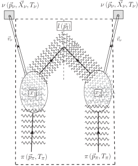
Figure 1: A space-time view of the product of the amplitude of the event that a neutrino is detected in a decay of a pion Eq. $(\ref{probability-correlation})$ is given. The pion and lepton are expressed by plane waves and the neutrino is by the wave packet of the size $\sigma_{\nu}$. The integrand is the product of the neutrino wave function of a velocity ${\vec{v}}_{\nu}$ and $\Delta_{\pi,l}(x_{1},x_{2})$ that corresponds to the diagram surrounded by a box of dot line.

$H_{0}+H_{\text{int}}$ in Eq. $(\ref{Schro. equation})$ is Hermitian, and the norm of the sate is preserved and $S[T]S^{\dagger}[T]=1$. This unitarity ensures the conservation of probability, i.e., a sum of the probability for finding the pion and the lepton and neutrino at a $t$ simultaneously. Furthermore, the charged lepton and corresponding neutrino have the same probability in this case. If the probabilities are measured independently of particles at $T$, there is no reason for them to be the same. The unitarity also does not connect the probability at $T$, $P(T)$, with that at $T^{\prime}$, $P({T}^{\prime})$. Consequently the decay rates could depend on both of $T$ and measured particles, and are computed with $S[T]$ of fulfilling the boundary conditions of experiments.

3 Position-dependent probability

We now study the probability of event that a neutrino is detected at a finite distance. The transition amplitude is the scalar product of the initial wave function with the final wave function that has the kinetic energy varying with time. The $S[T]$ and probability reflect this property and show non-uniform behavior, which is not computable correctly with $S[\infty]$. Details of the derivations are explained in Refs. [18, 36].

3.1 High-energy pion

The decay of a plane wave of pion to a plane wave of lepton and a wave packet of neutrino is expressed with a matrix element of $S[T]$ between a state composed of the neutrino of ${\vec{p}}_{\nu}$ at $\vec{{X}}_{\nu}$ and the charged lepton $l$ of ${\vec{p}}_{l}$ and the initial pion at $t={T}_{\pi}$ of ${\vec{p}}_{\pi}$, Fig. 1, is expressed as $\mathcal{M}=\int d^{4}x\,\langle{l},{\nu}|H_{\text{int}}(x)|\pi\rangle$, where $|\pi\rangle=|{\vec{p}}_{\pi},{T}_{\pi}\rangle,\ |l,\nu\rangle=|\vec{p}_{l};\vec{p}_{\nu},\vec{{X}}_{\nu},{T}_{\nu}\rangle$. In high energy, the life-time of the pion becomes long and can be ignored. $\mathcal{M}$ is then written with the matrix element of $V-A$ current of pion, Eq. $(\ref{pion-coupling})$, and Dirac spinors

$$\mathcal{M}=\int d^{4}xN_{1}\langle 0|J_{V-A}^{\mu}(0)|\pi\rangle\bar{u}({\vec{p}}_{l})\gamma_{\mu}(1-\gamma_{5})\nu(x,{\vec{p}}_{\nu},{\vec{X}}_{\nu},T_{\nu})\exp\left[-i(p_{\pi}-p_{l})\cdot x/\hbar\right],$$ (29)

$$\nu(x,{\vec{p}}_{\nu},{\vec{X}}_{\nu},T_{\nu})=\left({\frac{\sigma_{\nu}}{\pi}}\right)^{\frac{3}{4}}\int d{\vec{k}}_{\nu}\sqrt{\frac{m_{\nu}}{E_{\nu}}}\exp\left[{i{k_{\nu}\cdot(x-{X}_{\nu})/\hbar}-\frac{\sigma_{\nu}}{2}({\vec{k}}_{\nu}-{\vec{p}}_{\nu})^{2}}\right]\nu({\vec{k}}_{\nu}),$$

where $N_{1}=ig\left({m_{l}}/{E_{l}}\right)^{\frac{1}{2}}((2\pi)^{3}2E_{\pi}V)^{-\frac{1}{2}}$ and $V$ is a normalization volume. The wave packet $\nu(x,{\vec{p}}_{\nu},{\vec{X}}_{\nu},T_{\nu})$ satisfies the free wave equation and decreases rapidly at $t=T_{\nu}$ with ${\vec{x}}-{\vec{X}}$ and satisfies the condition for $f({\vec{x}},t)$ in Eq. $(\ref{basis-expansion})$ . For $t\leq T_{\nu}$,

$$\nu(x,{\vec{p}}_{\nu},{\vec{X}}_{\nu},T_{\nu})=\left({4\pi\over\sigma_{\nu}}\right)^{\frac{3}{4}}\sqrt{\frac{m_{\nu}}{E_{\nu}(p_{\nu})}}e^{ip_{\nu}\cdot(x-X_{\nu})/\hbar-\frac{1}{2\sigma_{\nu}}({\vec{x}}-{\vec{X}}_{\nu}-{\vec{v}}_{\nu}(t-T_{\nu}))^{2}}\left\{1+O({p_{\nu}^{-1}})\right\},$$ (30)

and the center moves with the velocity ${\vec{v}}_{\nu}={\vec{p}}_{\nu}c^{2}/{E_{\nu}}$, $\vec{x}_{\,0}=\vec{{X}}_{\nu}+{\vec{v}}_{\nu}(t-{T}_{\nu})$. We ignore $O({p_{\nu}^{-1}})$ term. The integrand of Eq. $(\ref{amplitude})$ becomes finite along a narrow space-time region of the velocity ${\vec{v}}_{\nu}$, and $t$ is integrated over ${T}_{\pi}\leq t\leq{T}_{\nu}$. ${\sigma_{\nu}}$ is the size of the neutrino wave packet [16, 17, 18]. For the sake of simplicity, we use the Gaussian form of the wave packet in this paper. The result for the finite-size correction is the same in general wave packets.

The total probability is an integral of a square of the modulus of the amplitude over the complete set of final states [15],

$$P=\int d\vec{{X}}_{\nu}{d{\vec{p}}_{\nu}\over(2\pi)^{3}}\frac{d{\vec{p}}_{l}}{(2\pi)^{3}}\sum_{s_{1},s_{2}}|\mathcal{M}|^{2},$$ (31)

where the momenta of the neutrino and charged lepton are integrated over the whole positive energy region, and the position of the wave packet is integrated over the region of the detector. This depends on ${T}={T}_{\nu}-{T}_{\pi}$. Hereafter the natural unit, $c=\hbar=1$, is taken in majority of places, but $c$ and $\hbar$ are written explicitly when it is necessary. Figure 1 shows the space-time configuration of the amplitude and probability expressed by the overlap of wave functions of the initial pion with those of lepton and neutrino.

Computation of the probability in a consistent manner with the Lorentz invariance was made with a correlation function $\Delta_{\pi,l}(x_{1},x_{2})$ of the pion and lepton vertex and the neutrino wave function. Integrating over the momentum ${\vec{p}}_{l}$ first, after summing over the spin, and we have the probability in the form

$$P =\int d\vec{{X}}_{\nu}{d{\vec{p}}_{\nu}\over(2\pi)^{3}}\frac{N_{2}}{E_{\nu}}\int d^{4}x_{1}d^{4}x_{2}\exp{\left[{-\frac{1}{2\sigma_{\nu}}\sum_{i}({\vec{x}}_{i}-\vec{x}_{i}^{\,0})^{2}}+i\phi(\delta x)\right]}\Delta_{\pi,l}(\delta x),$$ (32)

$$\vec{x}_{i}^{\,0} =\vec{{X}}_{\nu}+{\vec{v}}_{\nu}(t_{i}-{T}_{\nu}),\ \delta x=x_{1}-x_{2},\ \phi(\delta x)=p_{\nu}\!\cdot\!\delta x,$$

where $N_{2}=g^{2}f_{\pi}^{2}\left({4\pi}/{\sigma_{\nu}}\right)^{\frac{3}{2}}((2\pi)^{3}2E_{\pi}V)^{-1}$, and

$$\Delta_{\pi,l}(\delta x)={\frac{1}{(2\pi)^{3}}}\int{d{\vec{p}}_{l}\over E({\vec{p}}_{l})}\left\{2(p_{\pi}\cdot p_{\nu})(p_{\pi}\cdot p_{l})-m_{\pi}^{2}(p_{l}\cdot p_{\nu})\right\}e^{-i(p_{\pi}-p_{l})\cdot\delta x}.$$ (33)

$\Delta_{\pi,l}(\delta x)$ becomes the sum of the light-cone singularity, $\delta({\delta x}^{2})$, and less singular and regular functions in the region $m_{\pi}^{2}\geq m_{l}^{2}$. $\Delta_{\pi,l}(\delta x)$ vanishes in $m_{\pi}^{2}<m_{l}^{2}$. $\Delta_{\pi,l}(\delta x)$ is then expressed as

$$\Delta_{\pi,l}(\delta x)= 2i\left\{m_{\pi}^{2}p_{\nu}\cdot\left(p_{\pi}+i\frac{\partial}{\partial\delta x}\right)-2i(p_{\pi}\cdot p_{\nu})\left(p_{\pi}\cdot\frac{\partial}{\partial\delta x}\right)\right\}$$

$$\times\left[\frac{\epsilon(\delta t)}{4\pi}\delta(\lambda)+I_{1}^{\text{regular}}+I_{2}\right],$$ (34)

where $\lambda=(\delta x)^{2}=\delta t^{2}-\delta\vec{x}^{\,2}$ and $I_{1}^{\text{regular}}$ is composed of Bessel functions (see Appendix B). $\epsilon(\delta t)$ is a sign function and $\delta(\lambda)$ is Dirac’s delta function. $I_{2}$ is regular. After tedious integrations over ${\vec{x}}_{i}(i=1,2)$ in Eq. $(\ref{probability-correlation})$, we have the slowly varying term from the light-cone singularity

$$J_{\delta(\lambda)}=C_{\delta(\lambda)}\frac{\epsilon(\delta t)}{|\delta t|}\exp\left[{i\bar{\phi}_{c}(\delta t)-\frac{m_{\nu}^{4}c^{8}}{16\sigma_{\nu}E_{\nu}^{4}}{\delta t}^{2}}\right],$$ (35)

$$C_{\delta(\lambda)}=\frac{{(\sigma_{\nu}\pi)}^{\frac{3}{2}}{\sigma_{\nu}}}{2},\ \bar{\phi}_{c}(\delta t)=\omega_{\nu}\delta t=\frac{m_{\nu}^{2}c^{4}}{2E_{\nu}}\delta t,$$

and rapidly decreasing or oscillating functions from $I_{1}^{\text{regular}}$. The phase $\phi(\delta x)$ that varies rapidly in $\delta t$ and $\delta{\vec{x}}$ in Eq. $(\ref{probability-correlation})$ became $\bar{\phi}_{c}(\delta t)$ of the slow angular velocity $\omega_{\nu}$ in $\bar{\phi}_{c}(\delta t)$ of Eq. $(\ref{lightcone-integration2-2})$ at the light cone $\lambda=0$. The next singular term is from ${1/\lambda}$ in $\Delta_{\pi,l}(\delta x)$, and becomes $J_{\delta(\lambda)}/\sqrt{\pi\sigma_{\nu}|\vec{p}_{\nu}|^{2}}$. This is much smaller than $J_{\delta(\lambda)}$ and is negligible in the present parameter region. The magnitude is inversely proportional to $|\delta t|$. This behavior is satisfied in general forms of the wave packets.

Finally we have the probability in the form,

$$P=\int d\vec{{X}}_{\nu}{d^{3}p_{\nu}\over(2\pi)^{3}}N_{3}\int dt_{1}dt_{2}\biggl{[}\frac{\epsilon(\delta t)}{|\delta t|}e^{i{\bar{\phi}_{c}(\delta t)}}+2D_{\tilde{m}}(p_{\nu}){\tilde{L}_{1}\over\sigma_{\nu}}-{2i\over\pi}\left({\sigma_{\nu}\over\pi}\right)^{\frac{1}{2}}\tilde{L}_{2}\biggr{]},$$

$$N_{3}=i{\sigma_{\nu}}g^{2}f_{\pi}^{2}p_{\pi}\!\cdot\!p_{\nu}(m_{\pi}^{2}-2p_{\pi}p_{\nu})(2E_{\pi}E_{\nu}V)^{-1},$$ (36)

where $D_{\tilde{m}}(p_{\nu})$ and $\tilde{L}_{2}$ are given in Appendix B. The first term in Eq. (3.1) oscillates extremely slowly with the angular velocity $\omega_{\nu}$. The remaining terms tend exponentially to zero or oscillating functions, as $|\delta t|\rightarrow\infty$. The first and second terms in the right-hand side of Eq. $(\ref{total-probability2})$ exist in the region

$$2p_{\pi}\!\cdot\!p_{\nu}\leq{\tilde{m}}^{2}=m_{\pi}^{2}-m_{l}^{2},$$ (37)

and vanish outside this region [2].

Integrations over $t_{1}$ and $t_{2}$ are made next. The slowly varying and rapidly varying terms, $\frac{1}{\delta t}e^{i\omega_{\nu}\delta t}$ and $I_{1}^{\text{regular}}$, give the probabilities of different behaviors. The integrations over $t_{1}$ and $t_{2}$ of the former term is

$$i\int_{0}^{{T}}dt_{1}dt_{2}\frac{\epsilon(\delta t)}{|\delta t|}e^{i{\omega_{\nu}}\delta t}={T}(\tilde{g}(\omega_{\nu}{T})-\pi),\$$ (38)

where the function $\tilde{g}(\omega_{\nu}{T})$ in the right-hand side satisfies $\tilde{g}(\omega_{\nu}{T})_{{T}=0}=\pi,\frac{\partial}{\partial{T}}\tilde{g}(\omega_{\nu}{T})|_{{T}=0}=-\omega_{\nu}$ and $\tilde{g}(\omega_{\nu}T)=\frac{2}{\omega_{\nu}T},\text{ for }\omega_{\nu}T\rightarrow\infty$. The last term in Eq. (38) is canceled by the integral of the short-range term $I_{1}^{\text{regular}}$. $\tilde{g}(\omega_{\nu}{T})$ is generated by the sum of infinite waves that results to the light-cone singularity, and we call this a diffraction term. The last term $I_{2}$ in Eq. $(\ref{muon-correlation-total})$ gives ${2\over\pi}\sqrt{\sigma_{\nu}\over\pi}\int dt_{1}dt_{2}\tilde{L}_{2}(\delta t)={T}G_{0}$, where the constant $G_{0}$ is computed numerically. Owing to the rapid oscillation, only the microscopic $|\delta t|$ contributes to this integral, and consequently $G_{0}$ is constant in a macroscopic $T$.

Integrating over $\vec{{X}}_{\nu}$, we obtain the total probability expressed as the sum of the normal term $G_{0}$ and the diffraction term $\tilde{g}(\omega_{\nu}{T})$:

$$P=N_{4}\int\frac{d\vec{p}_{\nu}}{(2\pi)^{3}}\frac{p_{\pi}\!\cdot\!p_{\nu}(m_{\pi}^{2}-2p_{\pi}\!\cdot\!p_{\nu})}{E_{\nu}}\left[\tilde{g}(\omega_{\nu}{T})+G_{0}\right],$$ (39)

where $N_{4}={T}g^{2}f_{\pi}^{2}\sigma_{\nu}(2E_{\pi})^{-1}$ and ${L}=c{T}$ is the length of the decay region. $P$ is the probability of the event that the neutrino is detected. The first term in the right-hand side corresponds to the energy-non-conserving term $S^{(d)}[{T};f]$, and the second term corresponds to the energy-conserving term $S^{(n)}[{T}]$. The former vanishes at ${T}\rightarrow\infty$, and is the finite-size correction, which is stable with respect to variation of the pion’s momentum.

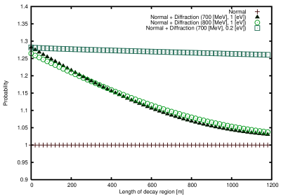
Figure 2: Total rate of the event that the muon neutrino is detected at a finite distance $L$ for $\tau_{\pi}=\infty$. The constant (red line) shows the normal term, and the diffraction term is given on top of the normal term. The horizontal axis represents the distance in meters, and the normal term is normalized to $1.0$. The neutrino mass, pion energy, and neutrino energy are 1.0 eV/$c^{2}$ or 0.2 eV/$c^{2}$, 4 GeV, and 700 (blue triangles) or  800 (green circles) MeV, respectively. The excess varies with the distance for $m_{\nu}=1.0$ eV/$c^{2}$ and is almost constant for $m_{\nu}=0.2$ eV/$c^{2}$.

Infinite number of states in $|\Psi(t)\rangle$ in Eq. $(\ref{pertubative-wave})$ of almost identical phases give the light-cone singularity to $\Delta_{\pi,l}(\delta x)$, and the finite-size correction expressed in $\tilde{g}(\omega_{\nu}{T})$. The present quantum mechanical effect remains at the macroscopic distance, $2c\hbar E_{\nu}/(m_{\nu}^{2}c^{4})$.

Next, we evaluate each term of Eq. $(\ref{probability-3})$. In $G_{0}$, approximately, $p_{\pi}=p_{l}+p_{\nu}$, and $2p_{\pi}\cdot p_{\nu}-m_{\pi}^{2}=m_{l}^{2}$. Integrating over the neutrino’s angle, we find that this term is independent of $\sigma_{\nu}$, which is consistent with the condition for the stationary state [24], and the rate agrees with the value obtained by the ordinary method. In $\tilde{g}(\omega_{\nu}{T})$, $p_{\pi}\neq p_{l}+p_{\nu}$, and the inner product, $p_{\pi}\cdot p_{\nu}$, is not expressed with the masses of pion and charged lepton. Instead, the convergence condition requires that this term is present in the kinematical region, $|\vec{p}_{\nu}|(E_{\pi}-|\vec{p}_{\pi}|)\leq p_{\pi}\!\cdot\!p_{\nu}\leq{\tilde{m}^{2}/2}$.

It is impossible to experimentally distinguish both components, therefore, we add both terms. The total probability thus obtained is presented in Fig. 2 for neutrino masses $m_{\nu}=1$ eV/$c^{2}$ and $0.2$ eV/$c^{2}$, a pion energy $E_{\pi}=4$ GeV of mean life-time $\tau_{\pi}=\infty$, and the neutrino energies $E_{\nu}=700$ and $800$ MeV. For the wave packet size of the neutrino, we use the size of the nucleus having a mass number $A$, $\sigma_{\nu}=A^{\frac{2}{3}}/m_{\pi}^{2}$. For the ¹⁶O nucleus, $\sigma_{\nu}=6.4/m_{\pi}^{2}$. From Fig. 2, we see that an excess varies with the distance for ${L}<1200$ m for $m_{\nu}=1$ eV/$c^{2}$ and is almost constant for $0.2$ eV/$c^{2}$ and that the maximal excess is approximately $20$% of the normal term at ${L}=0$. The slope at the origin ${L}=0$ is determined by $\omega_{\nu}$. The diffraction term varies slowly with both distance and energy. For this situation, the typical length is ${L}_{0}~{}[\text{m}]=2E_{\nu}\hbar c/(m_{\nu}^{2}c^{4})=400\times{E_{\nu}[\text{GeV}]/m_{\nu}^{2}[\text{eV}^{2}/c^{4}]}$. The neutrino’s energy is measured experimentally with uncertainty $\Delta E_{\nu}$, which is of the order of $0.1\times E_{\nu}$. This uncertainty is $100$ MeV for $1$ GeV neutrino energy and the diffraction components of both energies are almost equivalent to those given in Fig. 2. For the case of larger energy uncertainty, the computation is easily done using Eq. (39).

Using the asymptotic behavior of $\tilde{g}(\omega_{\nu}T)={2\over\omega_{\nu}T}$, we find an analytic expression of the correction, although the precise form of $\tilde{g}(\omega_{\nu}T)$ is used in comparing the theory with the experiments. The rate, is expressed with the $\Gamma_{0}$ of Eq. $(\ref{life-time})$ and this correction as

$$\Gamma(T,\sigma_{\nu})=\Gamma_{0}+\Gamma^{\text{diff}}(T,\sigma_{\nu}),$$ (40)

$$\Gamma^{\text{diff}}(T,\sigma_{\nu})=\frac{G_{F}^{2}f_{\pi}^{2}}{320\pi^{2}}m_{\pi}^{4}\left(1-\frac{m_{l}^{2}}{m_{\pi}^{2}}\right)^{4}\left(1+\frac{4m_{l}^{2}}{m_{\pi}^{2}}\right){m_{\pi}^{2}\sigma_{\nu}p_{\pi}\over Tm_{\nu}^{2}}{1\over E_{\pi}}.$$

$\Gamma^{\text{diff}}(T,\sigma_{\nu})$ depends on $T$ and $\sigma_{\nu}$, and decreases with $T$ for a fixed $\sigma_{\nu}$, and increases with $\sigma_{\nu}$ for a fixed $T$. The asymptotic value $\lim_{T\rightarrow\infty}\Gamma(T,\sigma_{\nu})$ is independent of $\sigma_{\nu}$ and is computed with plane waves of $\sigma_{\nu}=\infty$, which agrees with those computed with $S[\infty]$ combined with $i\epsilon$ prescription. It is noted that,

$$\lim_{\sigma_{\nu}\rightarrow\infty}\left\{\lim_{T\rightarrow\infty}\Gamma(T,\sigma_{\nu})\right\}=\Gamma_{0},$$ (41)

$$\lim_{T\rightarrow\infty}\left\{\lim_{\sigma_{\nu}\rightarrow\infty}\Gamma(T,\sigma_{\nu})\right\}=\infty.$$ (42)

The fact that Equation $(\ref{limit2})$ diverges is consistent with the behavior of the coefficient of $1/T$ term in Fermi’s golden rule given in Appendix. $c{T}\gg\sigma_{\nu}$ has been studied often and Equation $(\ref{limit1})$ is applied. $\sigma_{\nu}\gg c{T}$ has been less studied but there are various places and Equation $(\ref{limit2})$ is applied. Due to diverging rate, intriguing phenomena may arise. Thus a careful consideration is necessary when $(\sigma_{\nu},T)\rightarrow(\infty,\infty)$ is studied.

3.1.1 Neutrino spectrum vs charged lepton spectrum

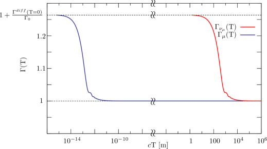
Figure 3: The event rates that the muon and muon neutrino are detected at a finite distance $L=cT$ for $\tau_{\pi}=\infty$. For the muon written with a blue line, the rate becomes the asymptotic value at $10^{-12}$ m, and for the neutrino written with a red line that becomes at $1000$ m. The horizontal axis represents the distance in meters, and the asymptotic value $\Gamma_{0}$ is normalized to $1.0$. The neutrino mass, pion energy, and neutrino energy are $E_{\pi}=4$ GeV, $E_{\nu}=800$ MeV, $m_{\nu}=1$ eV/$c^{2}$, $\sigma$: ${}^{16}O$. The detector’s size is not considered.

In pion decays, the lepton and neutrino are produced in pair by the local weak interaction $H_{\text{int}}$ and the wave function $|\Psi(t)\rangle$ in Eq. $(\ref{pertubative-wave})$ expresses the whole system, and the norm of parent wave function decreases with the average life-time $\tau_{\pi}$ and that of the daughters increases with the same $\tau_{\pi}$. Experiments observe the events that the daughters are detected and the probability is computed with the amplitude that is defined according to this boundary condition, which becomes different at a finite $T$ from $\tau_{\pi}$ of Eq. $(\ref{pertubative-wave})$. Because the neutrino has almost the constant phase and group velocity, its wave packet keeps coherence and retains the interference pattern for long distance. When the neutrino is detected in this wave zone, the event rate is amplified of revealing the finite-size correction. The leptons, on the other hand, are massive and have the velocities that vary with the momentum, and the wave packet does not show the strong effect.

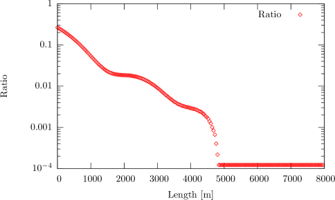
Figure 4: The ratio of the event rate Eq. $(\ref{nue/numu})$ that the electron neutrino is detected over that the muon neutrino is detected. The value varies from $0.2$ at $\text{L}=0$ to $10^{-4}$ at $\text{L}=\infty$ slowly. The horizontal axis represents the distance in meters. The neutrino mass, pion energy, and neutrino energy are 1.0 eV/$c^{2}$ , 4 GeV, and 800 MeV, respectively. The detector’s size is not considered.

In fact, $\Gamma^{diff}(T,\sigma_{i});i=\nu,l$ in Eq. $(\ref{rate-general})$ is inversely proportional to the mass-squared and is large for the neutrino $i=\nu$ and is small for the charged leptons $i=l$ if $\sigma_{l}\approx\sigma_{\nu}$. Thus the rates at $T=0~{}\text{and}~{}\infty$ , for $\sigma_{\nu}=\sigma_{l}=\sigma$, satisfy

$$\Gamma(T=\infty,\sigma_{\nu}=\sigma;neutrino)=\Gamma(T=\infty,\sigma_{l}=\sigma;lepton),$$ (43)

$$\Gamma(T=0,\sigma_{\nu}=\sigma;neutrino)=\Gamma(T=0,\sigma_{l}=\sigma;lepton),$$ (44)

but at finite $T$, they are different. Figure 3 shows them. The finite-size correction appears even at a macroscopic $T$ for the neutrinos, and appears only at a microscopic $T$ for the charged leptons. Even though they are produced in pair, they propagate differently and are detected with the different rates due to the finite-size corrections. The ratio varies from $10^{-4}$ at $T=\infty$ to $0.2$ at $T=0$. The enhancement of electron mode at finite $T$ is huge.

3.1.2 Suppression of electron mode

The ratio of the event that the electron is detected over the event that the muon is detected at $T=\infty$ is

$$\Gamma_{0}(electron)/\Gamma_{0}(muon)={m_{e}^{2}\over m_{\mu}^{2}}\left(1-{m_{\mu}^{2}\over m_{\pi}^{2}}\right)^{-2}=1.28\times 10^{-4},$$ (45)

which is consistent with the experimental value $1.23\times 10^{-4}$. The suppression of the electron mode played the important role to prove the form of interaction to $V-A$ type. The branching ratio vanishes for massless charged lepton because they have opposite helicities and decouple from scalar or pseudo-scalar particle. Thus the conservation law of kinetic energy and angular momentum, which hold at $T=\infty$, suppresses the electron mode. Now the finite-size correction comes from the final states of the non-conserving kinetic energy, hence does not follow the helicity suppression. The probabilities of the events that the charged leptons are detected at $cT=10^{-10}$ m agree with the asymptotic values of Eq. $(\ref{helicity-suppression})$. Whereas, the ratio of the probabilities of the events that the electron neutrino is detected over that the muon neutrino is detected at a $T$,

$$R_{e}(T)=\Gamma(T,\nu_{e})/\Gamma(T,\nu_{\mu})$$ (46)

becomes very different from Eq. $(\ref{helicity-suppression})$ due to the large finite-size corrections, $\Gamma^{\text{diff}}(T,\sigma)$ in Eq. $(\ref{rate-general})$. The ratio of the total number of events, which is slightly different from the experimental value due to the finite size of the detector, at finite $T$ for 1.0 eV/$c^{2}$ , 4 GeV, and 800 MeV for the neutrino mass, pion energy, and neutrino energy is shown in Fig. 4. In Fig. 4, the ratio of probabilities integrated over the whole angles are plotted, and is considered the maximum value.

The ratio varies from $10^{-4}$ at $T=\infty$ to $0.2$ at $T=0$. The enhancement of electron mode at finite $T$ is huge. In real experiments, the detectors of finite sizes are used. The values then become smaller, and become consistent with existing values within experimental uncertainties. Later we compare theoretical values with experimental data, then the size and geometry of detector are included.

3.2 Intermediate-energy pion

So far we have studied the high-energy pion whose life-time is ignorable, and one flavor neutrino. Hereafter the pion’s life-time and three flavor are included. The pion’s life-time gives the damping factor $e^{-\frac{t_{1}+t_{2}}{\tau_{\pi}}}$ to the left-hand side of Eq. $(\ref{probability1})$. The new universal function $\tilde{g}(\omega_{\nu},{T};\tau_{\pi})$

$$i\int_{0}^{{T}}dt_{1}dt_{2}\frac{\epsilon(\delta t)}{|\delta t|}e^{i{\omega_{\nu}}\delta t-{t_{1}+t_{2}\over\tau_{\pi}}}=\tilde{g}(\omega_{\nu},{T};\tau_{\pi})-\tilde{g}_{0};\ T>{\sqrt{\sigma}_{\nu}\over c},$$ (47)

where $\tilde{g}(\omega_{\nu},\infty,\tau_{\pi})=0$, replaces $T\tilde{g}(\omega_{\nu}{T})$, and $(1-e^{-{T}/\tau_{\pi}})G_{0}$ replaces $TG_{0}$.

The integrand of Eq. $(\ref{probability2})$ proportional to

$$\exp\left[(i\omega_{\nu}-{1/\tau_{\pi}})t_{1}\right]\times\exp\left[(-i\omega_{\nu}-{1/\tau_{\pi}})t_{2}\right],$$ (48)

shows that a motion is equivalent to a damped oscillator of the angular velocity $\omega_{\nu}$ and the decay rate ${1\over\tau_{\pi}}$. Now for $E_{\nu}=1$ GeV their values are,

$$\hbar\omega_{\nu} =\begin{cases}10^{-9}\ \text{eV},\ \text{for}~{}m_{\nu}=1\ \text{eV}/c^{2},\\ 10^{-11}\ \text{eV},\ \text{for}\ m_{\nu}=0.1\ \text{eV}/c^{2},\end{cases}$$ (49)

$${\hbar\over\tau_{\pi}} =\begin{cases}3\times 10^{-8}\ \text{eV},\ \text{at rest},\\ 1.5\times 10^{-10}\ \text{eV},\ E_{\pi}=50m_{\pi}c^{2}.\end{cases}$$ (50)

The motion is sensitive to $\omega_{\nu}$ in the region of $\omega_{\nu}\approx{1\over\tau_{\pi}}$. Now $\omega_{\nu}$ is proportional to the square of the absolute value of neutrino mass, thus $P$ is useful to probe it around $m_{\nu}=0.1$ eV/$c^{2}$. Mass-squared differences $\delta m^{2}_{\nu}$ are extremely small [3, 11, 12], and their central value is currently unknown. If that is in the above range, the probability in the region $T\leq\tau_{\pi}$ can be used to measure the absolute neutrino mass.

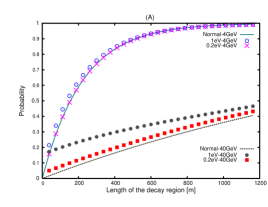
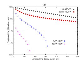
Figure 5: Probability of the event that the neutrino is detected at distance $L$ for $E_{\pi}=4$ and $40$ GeV. In (A), solid green ($4$ GeV) and dotted black line ($40$ GeV) represent the normal and diffraction terms, respectively, for for $m_{\nu}$ of $0.2$ and $1.0$ eV/$c^{2}$. The diffraction terms are written on top of the normal terms. Values are normalized to one at ${L}=\infty$. In (B), fractions of diffraction terms that vary with pion’s energy and neutrino mass are shown. The horizontal axis represents distance in [m]. Neutrino energy is 700 MeV. The detector’s size is not considered.

The probabilities of the events for several parameters are given in Fig. 5. The finite-size correction becomes smaller for lower energy and the life-time effect becomes significant for smaller neutrino mass. Thus the fraction becomes sensitive to the neutrino mass and negligibly small in low energy pion in ${L}>200$ m, if the mass is less than $0.05$ eV/$c^{2}$. For three neutrinos of masses $m_{{\nu}_{i}};i=1-3$ and a mixing matrix $U_{i,\alpha};\alpha=e,\mu,\tau$, the Lagrangian Eq. $(\ref{lagrangian})$ is modified to that of three neutrino $\nu_{i}(x);i=1-3$ of the masses $m_{{\nu}_{i}}$ and the weak current

$$J_{V-A}(x)={J_{V-A}}^{i}(x)U_{i,\alpha}.$$ (51)

The amplitude for the neutrino of flavor $\alpha$ and the charged lepton $l$ is given by

$$\mathcal{M}=\sum_{i}U_{l,i}\mathcal{M}(l,i)U_{i,\alpha}^{\dagger},$$ (52)

and the probability is

$$P = \sum_{l=e,\mu}\int d{\vec{X}}_{\nu_{\alpha}}{d{\vec{p}}_{\nu_{\alpha}}\over(2\pi)^{3}}{d{\vec{p}}_{l}\over(2\pi)^{3}}|\mathcal{M}|^{2}$$ (53)

$$= \sum_{l=e,\mu}\int d{\vec{X}}_{\nu_{\alpha}}{d{\vec{p}}_{\nu_{\alpha}}\over(2\pi)^{3}}{d{\vec{p}}_{l}\over(2\pi)^{3}}|U_{l,i}\mathcal{M}(l,i)U_{i,\alpha}^{\dagger}|^{2},$$

where $\mathcal{M}(l,i)$ is the amplitude for the mass eigenstate $i$. $P$ of Eq. $(\ref{three-f-probability})$ includes the diffraction and normal terms. The diffraction term exists in the kinematical region of ${\vec{p}}_{\nu_{\alpha}}$ satisfying the condition Eq. $(\ref{convergence})$, which depends on the charged lepton’s mass, and is independent of the species in its form. Thus the diffraction term in

$$\int\frac{d{\vec{p}}_{l}}{(2\pi)^{3}}\mathcal{M}(l,i)\mathcal{M}^{*}(l,j)$$ (54)

does not depend on $l$. The phase of the integrand in Eq. $(\ref{probability2})$ is replaced with the phase, ${\omega_{\nu_{i}}+\omega_{\nu_{j}}\over 2}(t_{1}-t_{2})+\frac{\omega_{\nu_{i}}-\omega_{\nu_{j}}}{2}(t_{1}+t_{2})$. The latter is much smaller than ${1\over\tau_{\pi}}(t_{1}+t_{2})$ in magnitude and can be ignored in the short distance region. Hence the diffraction in Eq. $(\ref{l-i-diffraction})$ is proportional to $\tilde{g}({\omega_{\nu_{i}}+\omega_{\nu_{j}}\over 2},T;\tau_{\pi})$. The normal term satisfies the conservation law of kinetic energy and momentum, and $m_{\pi}^{2}-2p_{\pi}\!\cdot\!p_{\nu_{\alpha}}=m_{l}^{2}$, hence the integrand in electron mode is negligible. Thus $l=\mu$ contributes. This depends on $i$ through $D_{i}({\vec{p}}_{\nu},T)=e^{i{(E_{\nu_{i}}({\vec{p}}_{\nu})T-p_{\nu}cT)}}$ and $U_{i,\alpha}$, and agrees with the standard oscillation formula.

In the kinematical region $V_{1}:2p_{\pi}\!\cdot\!p_{\nu}\leq m_{\pi}^{2}-m_{\mu}^{2}$, the convergence condition Eq. $(\ref{convergence})$ for $l=e,\mu$ is satisfied, and we have the probability of the event that the neutrino of flavor $\alpha$ is detected,

$$P = \frac{N_{4}}{T}\int_{V_{1}}{d\vec{p}_{\nu_{\alpha}}\over(2\pi)^{3}}\frac{p_{\pi}\!\cdot\!p_{\nu_{\alpha}}(m_{\pi}^{2}-2p_{\pi}\!\cdot\!p_{\nu_{\alpha}})}{E_{\nu_{\alpha}}}\sum_{i}$$

$$\times\left[\sum_{j,l}U_{ij}^{\alpha}(U_{ji}^{l})^{*}\tilde{g}(\omega_{i,j},{T};\tau_{\pi})+|U_{l,i}D_{i}({\vec{p}}_{\nu_{\alpha}},T)U^{\dagger}_{\alpha,i}|^{2}G_{0}(1-e^{-T/\tau_{\pi}})\right],$$

$$U_{ij}^{\alpha}=U_{i,\alpha}^{\dagger}U_{j,\alpha},\ \omega_{ij}={\omega_{\nu_{i}}+\omega_{\nu_{j}}\over 2},$$

where $E_{\nu_{\alpha}}=p_{\nu_{\alpha}}$ can be used except in $D_{i}({\vec{p}}\,)D_{j}^{*}({\vec{p}}\,)=e^{i\frac{m_{\nu_{i}}^{2}-m_{\nu_{j}}^{2}}{2p}{T}}$.

In the kinematical region $V_{2}:m_{\pi}^{2}-m_{\mu}^{2}\leq 2p_{\pi}\cdot p_{\nu}\leq m_{\pi}^{2}-m_{e}^{2}$, the convergence condition Eq. $(\ref{convergence})$ for $l=e$ is satisfied, and the diffraction gives a contribution. The normal term is negligible. Thus we have

$$P=\frac{N_{4}}{T}\int_{V_{2}}{d\vec{p}_{\nu_{\alpha}}\over(2\pi)^{3}}\frac{p_{\pi}\!\cdot\!p_{\nu_{\alpha}}(m_{\pi}^{2}-2p_{\pi}\!\cdot\!p_{\nu_{\alpha}})}{E_{\nu_{\alpha}}}\sum_{i,j}U_{ij}^{\alpha}(U_{ji}^{e})^{*}\tilde{g}(\omega_{ij},{T};\tau_{\pi}),$$ (56)

Equations. $(\ref{three-flavor})$ and $(\ref{three-flavor2})$ are the formula for the probability of the event of the neutrino $\alpha$ at the distance $c{T}$. The second term in the right-hand side of Eq. $(\ref{three-flavor})$ is the standard flavor oscillation term that depends on the mass-squared difference. The rests are the diffraction terms that depend on the square of average mass, $\omega_{ij}={m_{\nu_{i}}^{2}+m_{\nu_{j}}^{2}\over 2}$. It is convenient to define the average squared-mass ${\bar{m}_{\nu}}^{2}$ from

$$\tilde{g}(\bar{\omega}_{\nu},{T};\tau_{\pi})=\sum_{i,j,l}U_{ij}^{\alpha}(U_{ji}^{l})^{*}\tilde{g}(\omega_{\nu_{i}},{T};\tau_{\pi}),\ \bar{\omega}_{\nu}={{\bar{m}_{\nu}}^{2}\over 2E_{\nu}},$$ (57)

where ${\bar{m}_{\nu}}$ agrees with the central mass $m_{0}$ if $m_{0}^{2}\gg\delta m^{2}_{\nu}$. At ${L}\leq c\tau_{\pi}$, the first term gives a large contribution for $\alpha=e$ , but a small correction for $\alpha=\mu$. At ${L}\gg c\tau_{\pi}$, the diffraction term disappears and the expression agrees with the standard flavor oscillation formula.

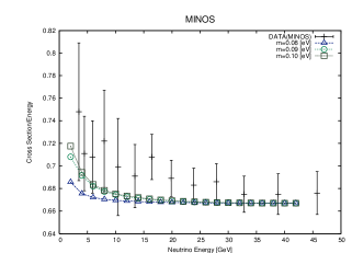
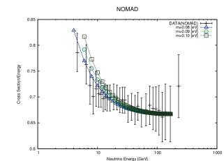
Figure 6: $\nu N$ total cross section from MINOS and NOMAD collaborations are compared with theory. Theory uses $\sigma_{\nu}=14.6/m_{\pi}^{2}$ of  ⁵⁶Fe, and geometry of MINOS and $\sigma_{\nu}=5.3/m_{\pi}^{2}$ of ¹²C, and geometry of NOMAD. The horizontal axis gives neutrino energy in GeV and the vertical axis gives the ratio of cross section to energy. The neutrino mass, $m_{\nu}=0.08,\ 0.09,\ 0.10$ eV/$c^{2}$, is used for theoretical calculation.

Now we compare experimental data with the theoretical values Eq. $(\ref{three-flavor})$. In Fig. 6, the total cross sections of high energy neutrino-nucleon scattering of the NOMAD [41] and MINOS [42] collaborations are presented. The geometry of each experiment is taken into account in the theoretical calculation and ${\sigma}_{\nu}=5.3/{m_{\pi}^{2}}$ or $14.6/{m_{\pi}^{2}}$ of ¹²C and ⁵⁶Fe are used. The theoretical values depend slightly on the neutrino mass and energy. In these high energy regions, the life-time of the parent does not give a significant effect and the corrections remain in the distances of these experiments. They give slight energy dependences to the total cross sections and agree with experiments. Other experiments except those discussed next are not in-consistent with the correction terms within experimental uncertainties.

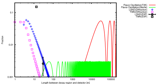
Figure 7: Theoretical fractions of the electron mode from the diffractions for LSND and TWN geometries are compared with LSND and TWN experiments. TWN(black box) and LSND(black circle) are the experimental values and magenta line of boxes is the value from diffraction for TWN of the parameters $m_{\nu}=0.2$ eV/$c^{2}$, $E_{\nu}=300$ MeV, and $p_{\pi}=1.4$ GeV/$c$. Blue cross line is the value for LSND with $m_{\nu}=0.1$ eV/$c^{2}$, $E_{\nu}=60$ MeV, and $p_{\pi}=400\,\text{MeV}/c$. Red line shows the value for flavor oscillation (T2K) for $\sin^{2}\theta_{13}=0.11$, $\delta m^{2}_{23}=2.4\times 10^{-3}\ \text{eV}^{2}/c^{4}$, and $E_{\nu}=60$ MeV. Green solid shows the value for the sterile neutrino for $\sin^{2}\theta=0.004$, $\delta m^{2}=1.2\ \text{eV}^{2}/c^{4}$, and $E_{\nu}=60$ MeV.

3.3 Neutrino mass from LSND

Next an anomaly on the fraction of electron mode over muon mode in the pion decay is compared. At ${L}/c\gg\tau_{\pi}$, the flavor diagonal term has the fraction of $10^{-4}$ [37, 38, 39, 40] and the value is determined by the flavor mixing term in Eq. $(\ref{three-flavor})$. Neutrino parameters determined in Ref. [3] as

$$|\delta m^{2}_{23}|=2.35^{+0.12}_{-0.09}\times 10^{-3},~{}\delta m^{2}_{21}=7.58^{+0.22}_{-0.26}\times 10^{-5}\ \text{eV}^{2}/c^{4},\ \sin^{2}\theta_{13}=0.096\pm 0.013,$$ (58)

are used. In the short distance region, the electron mode due to the diffraction has a significant fraction. Its magnitude is about 0.1 to $10^{-4}$ depending the neutrino mass and the distance from Figs. 4 and 5. Thus, the excess becomes enormous. Figure 7 shows the fraction that includes geometrical configurations of detectors. The value is about $0.05$ at a distance of a few meters and $0.01$ at a distance of 10 to 100 meters. That becomes negligible in a distance above 1000 meters. Thus the diffraction gives the dominant contribution in the short distance region and the flavor oscillation gives the dominant contribution in the long distance region.

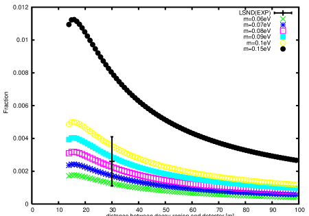
Figure 8: Relative fraction of the electron mode computed theoretically for LSND geometry is compared with the experiment. The neutrino mass is from $0.06$ eV/$c^{2}$ to $0.15$ eV/$c^{2}$, and $\sigma_{\nu}=5.3/{m_{\pi}^{2}}$ from ¹²C. The energies are $E_{\nu}=60$ MeV, and $p_{\pi}=400$ MeV/$c$. LSND (EXP) is consistent with the mass $m_{\nu}=0.082~{}\pm 0.020$ eV/$c^{2}$.

There have been several experiments in short distance regions. The first high-energy neutrino experiment, TWN [43], and the first liquid-scintillator experiment, LSND [44], detected the neutrinos in this region and modern experiments followed. TWN and LSND are compared with the theories of the flavor oscillations and the neutrino diffraction in Fig. 7. The experiments of TWN and LSND are not consistent with the flavor oscillations. For the LSND experiment, the distance is about 30 meters and the fraction of the electron neutrino and those of the flavor oscillation and the diffraction are plotted in Fig. 7. The oscillation probability with the mass-squared difference of Eq. $(\ref{flavour-parameter})$ (red line) vanishes, and that with a much larger value $\delta m^{2}=1.2\ \text{eV}^{2}/c^{4}$ (green line) agrees with the experiment. Obviously this value is much larger than the values of global fit for three neutrinos. Now the diffraction component (blue line) with $\sigma_{\nu}=5.3/{m_{\pi}^{2}}$ from ¹²C used in the target agrees with the experiment with the absolute neutrino mass around $0.08$ eV/$c^{2}$. Thus, we consider that the LSND event is a signal of neutrino diffraction. In Fig. 8, we compare the experiment with the theoretical values with the above wave packet size. They agree with the neutrino mass $\bar{m}_{\nu}=0.082\pm 0.020$ eV/$c^{2}$. MiniBooNE [46] tested LSND later at a different distance $L=490$ m and higher energy and did not see the signal expected from the flavor oscillation hypothesis of LSND. At this distance, the diffraction component with $\sigma_{\nu}=5.3/{m_{\pi}^{2}}$ from ¹²C for MiniBooNE becomes much smaller than that of LSND. Recent new data from MiniBooNE [47] claimed the anomaly in $L/E$ plot, and are compared in Fig. 9. The value is slightly larger than the diffraction of $\bar{m}_{\nu}=0.082\pm 0.020$ eV/$c^{2}$. However, the diffraction of neutrino from muon decay was not included in the background estimation. The present value, hence, is consistent with the diffraction of $m_{\nu}=0.082\pm 0.020$ eV/$c^{2}$. Thus MiniBooNE’s new and old data are consistent with the diffraction. The large signal for LSND and small signal for MiniBooNE are consistent with the neutrino diffraction.

Excess of shower events in TWN [43], which may be caused by the electron neutrino, are compared in Figs. 7 and 9. The fraction of shower events of TWN is slightly larger than those of theory. However, shower events in TWN might include the electron neutrino from the muon decay, which is furthermore amplified by the neutrino diffraction, [48]. Hence the experimental values are consistent with the theory using the mass obtained from LSND from Fig. 9.

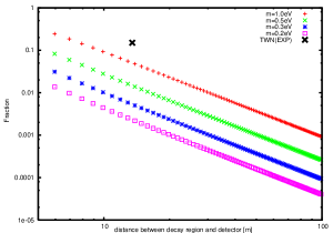
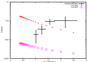
Figure 9: Relative fraction of the electron mode computed theoretically for TWN and MiniBooNE geometries are compared with experiments. The neutrino mass is from $0.2$ eV/$c^{2}$ to $1.0$ eV/$c^{2}$, and $\sigma_{\nu}=8.8/{m_{\pi}^{2}}$ or $5.3/{m_{\pi}^{2}}$ from ²⁶Al or¹²C. The error of TWN value is unknown, and the background estimation of MiniBooNE will be altered with the diffraction of the muon decay, hence the data are consistent with the theoretical values calculated with $m_{\nu}\approx 0.082~{}\pm 0.020$ eV/$c^{2}$, $E_{\nu}=300$ MeV, $p_{\pi}=1.4$ GeV/$c$ for TWN and $E_{\nu}=200-800$ MeV, $p_{\pi}=3$ GeV/$c$ for MiniBooNE.

MiniBooNE for the decay at rest and reactor experiments in a short distance also observed anomalies, which may be attributed to the neutrino diffraction. Nevertheless the precise quantitative analysis are not straightforward, since matter effects are more involved in these processes, and they will be studied in a separate publication. Further experiments at shorter distance may be able to confirm the diffraction of the electron neutrino.

From Eq. $(\ref{flavour-parameter})$, $\sqrt{\delta m_{23}^{2}}$ is slightly smaller than the average value, $0.082$ eV/$c^{2}$, and is larger than the error $0.020$ eV/$c^{2}$, and $\sqrt{\delta m_{21}^{2}}$ is much smaller than both. Hence the pattern of masses are either the normal or inverted hierarchies.

Now we substitute the mixing matrix $U$ determined from the global fits [3], to Eq. $(\ref{average-mass})$ and have the light and heavy masses,

$$m_{\nu_{L}}=0.085\pm 0.022\ \text{eV}/{c^{2}},\ m_{\nu_{H}}=0.098\pm 0.022\ \text{eV}/{c^{2}};\ \text{I},$$ (59)

$$m_{\nu_{L}}=0.070\pm 0.026\ \text{eV}/{c^{2}},\ m_{\nu_{H}}=0.083\pm 0.026\ \text{eV}/{c^{2}};\ \text{II},$$ (60)

and the sum of masses

$$\sum_{i}m_{\nu_{i}}=0.268\pm 0.078\ \text{eV}/{c^{2}};\ \text{I},$$ (61)

$$\sum_{i}m_{\nu_{i}}=0.236\pm 0.066\ \text{eV}/{c^{2}};\ \text{II},$$ (62)

for the normal (I) or inverted (II) mass hierarchies.

Thus the probability of the detection process of the pion decay at the distance ${L}=cT$ is computed by $S[{T}]$ as Eqs. $(\ref{probability-3})$ or $(\ref{three-f-probability})$, and deviates from that at ${L}=\infty$ given by $S[\infty]$. The probability has the large finite-size correction. If the charged lepton is observed simultaneously, the detection rate of the lepton has also the large finite-size correction. This result is different from the probability of the event that only charged lepton is detected but does not contradict with that of ordinary experiments, because the boundary conditions are different in two cases.

The finite-size correction of the probability of the event that only a charged lepton is detected is computed with $S[{T}^{\prime}]$ which satisfies the boundary condition for the charged lepton. Here ${T}^{\prime}={T}_{l}-{T}_{\pi}$ is the time interval for observing the charged lepton and the probability is expressed by Eq. $(\ref{probability-3})$ with $\omega_{\nu}\rightarrow\omega_{l}=m_{l}^{2}c^{4}/(2E_{l}\hbar)$. Since charged leptons are heavy, $\omega_{l}{T}^{\prime}$ becomes very large and $\tilde{g}(\omega_{l}{T}^{\prime})$ becomes ${2\over\omega_{l}T}\approx 0$ for macroscopic ${T}^{\prime}$. Thus, the probability does not have a finite-size correction and agrees with that of the normal term. Although the light-cone singularity forms in both cases, the diffraction component becomes relevant only when the detected particle is very light.

The probability of the event that a charged lepton is detected depends on the boundary condition of the neutrino. When a neutrino is detected at ${T}_{\nu}$, the charged-lepton spectrum includes the diffraction component but, when the neutrino is not detected, the charged-lepton spectrum does not include the diffraction component. The latter result is standard, whereas the former is not, but may be verified experimentally.

We now compare the finite-size correction with the diffraction of light passing through a hole. The former is that of a quantum mechanical wave and appears in the transition amplitude. The amplitude is determined by the initial and final states, and the time interval. The diffraction pattern forms in a direction parallel to the momentum of the non-stationary wave. The size determined by $\omega_{\nu}$ is extremely large for light particles and stable with respect to variations of the energy and other parameters. Consequently the diffraction is easily observed without fine tuning. Now the latter diffraction is that of a classical wave and appears in its intensity. The diffraction forms in a direction perpendicular to the momentum and with a phase difference $\omega_{\gamma}^{dB}\delta t$ where $\omega_{\gamma}^{dB}=c|\vec{p}_{\gamma}|/\hbar$ of the stationary wave. Its shape is determined by $\omega_{\gamma}^{dB}$, which is large and varies rapidly when the parameters are changed. Thus, the initial energy must be fine tuned to observe the diffraction of light.

4 Summary and future prospects

We found that the finite-size correction to the probability of the events that the neutrino from the pion decay is detected at a finite $T$ can be used to measure the neutrino absolute mass. The large corrections of unusual properties are caused by the Schrödinger equation and computed by $S[T]$ that satisfies the boundary condition of a finite $T$.

The neutrino energy spectrum and other patterns are determined by the difference of angular velocities, $\omega_{\nu}=\omega_{\nu}^{E}-\omega_{\nu}^{dB}$, where $\omega_{\nu}^{E}={E_{\nu}/\hbar}$ and $\omega_{\nu}^{dB}={c|\vec{p}_{\nu}|/\hbar}$. The $\omega_{\nu}$ takes the extremely small value ${m_{\nu}^{2}c^{4}}/{(2E_{\nu}\hbar)}$ because of the unique neutrino features [3, 11, 12]. Consequently, the correction term becomes finite in the macroscopic spatial region of $r\leq\frac{2\pi E_{\nu}\hbar c}{m_{\nu}^{2}c^{4}}$ and affects experiments in the mass-dependent manner at near-detector regions.

The dominant part of probability of the event that the electron neutrino is detected in this region is the correction term and has many unusual properties. Unfortunately, the measurement is not easy, because the identification of the electron neutrino and the neutrino experiment in this region itself are extremely hard. Hence the precision experiments have not been made in this region except LSND so far, and the predicted effects are not in-consistent with the existing data. This is a future problem.

Excesses of the events are observed by K2K [45], MiniBooNE [46, 47] and MINOS [49], and the excess in electron neutrinos known as the LSND anomaly were shown consistent with the finite-size corrections. Because the finite-size correction are independent of flavor oscillations, we found the absolute mass around $0.082\pm 0.020$ eV, Eqs. $(\ref{masses1})$ and $(\ref{masses2})$ from LSND. They resolve the controversy between LSND with others [54]. We compared all previous neutrino experiments and found that the new contribution in near-detector regions derived from the neutrino diffraction is surprisingly consistent with all of them. It would be important to confirm the neutrino diffraction and the absolute neutrino mass with precision experiments. The mass $0.082\pm 0.020$ eV/$c^{2}$ is close to the values suggested by other experiments or observations. Recent neutrino-less double $\beta$-decay experiment at KamLAND-Zen [50] gave a value $0.12-0.25$ eV/$c^{2}$ for the upper bound of the Majorana neutrino mass. Further observations may be able to confirm if the neutrino is Dirac or Majorana particle. The bounds from cosmology, $0.24$ eV/$c^{2}$ [3], $\sum_{i}m_{\nu_{i}}\leq 0.44$ eV/$c^{2}$ [12, 51], and $\sum_{i}m_{\nu_{i}}\leq 0.23$ eV/$c^{2}$ [52], are also close to the present value within three flavor [3, 53]. Thus the masses Eqs. $(\ref{masses1})$, $(\ref{masses2})$, $(\ref{sum-masses1})$, and $(\ref{sum-masses2})$ are consistent with existing data.

The probability determined by the diffraction around the overlapping region of wave functions of parent and daughters gives the finite-size correction and its magnitude depend on the size of wave functions that the neutrino interact with. We have used the values from the sizes of bound nucleus, $\sigma_{b}$, in targets in Eqs. $(\ref{masses1}),\ (\ref{masses2}),\ (\ref{sum-masses1}),\text{ and }(\ref{sum-masses2})$. If they are extended and have larger sizes of wave functions, the larger values, $\sigma_{m}$, are used. In this case, the absolute mass becomes

$$m_{\nu_{i}}=m^{b}_{\nu_{i}}({\sigma_{m}\over\sigma_{b}})^{1/2},$$ (63)

where $m^{b}_{\nu_{i}}$ shows the mass values Eqs. $(\ref{masses1}),\ (\ref{masses2}),\ (\ref{sum-masses1}),\text{ and }(\ref{sum-masses2})$. Since

$$\sigma_{m}\geq\sigma_{b}$$ (64)

the mass values Eqs. $(\ref{masses1}),\ (\ref{masses2}),\ (\ref{sum-masses1}),\text{ and }(\ref{sum-masses2})$ are considered the lower bounds. A future precision experiment in the short distance region of detecting the electron neutrino may be able to test the correction and give the precise masses.

We described a new method derived from quantum wave-like phenomenon specific to the extremely light particle, and showed the new physical observable. The effect of the transition amplitude was studied in the lowest order in $G_{F}$. Because that is independent of and not cancelled with higher order corrections, the effects due to a propagator of $W^{\pm}$ and higher order corrections of the renormalized theory do not modify the amplitude in the lowest order in $W$’s mass, $M_{W}$, and the light-cone singularity, hence our results are kept intact by them. A similar enhancement of $10^{4}$ or more caused by matter effect has been observed in various area [59]. Other large-scale quantum phenomena will be studied in subsequent presentations.

Appendix A The finite-size correction to Fermi’s Golden rule

In computing a scattering cross section and decay rate with Fermi’s Golden rules, the $1/T$ correction to the following formula for a large $T$ for a smooth function $g(\omega)$,

$$\int d\omega g(\omega)\left({\sin\left({\omega{T}}/{2}\right)\over\omega}\right)^{2}={T}\int dx\,g\left({x}/{{T}}\right)\left({\sin(x/2)\over x}\right)^{2}=2\pi Tg(0),$$ (A.1)

[55, 56] diverges if an expansion, $\displaystyle g\left({x}/{{T}}\right)=g(0)+\sum_{l}\frac{g^{(l)}(0)}{l!}\left(\frac{x}{{T}}\right)^{l}$ is substituted. The diverging integral becomes finite with a use of boundary condition. Eq. (29) is such amplitude that satisfies the boundary conditions at $T$, and gives the unique finite-size correction.

Appendix B Light cone singularity.

Innumerable states at the ultra-violet energy region in a relativistic invariant system lead the correlation function $\Delta_{\pi,l}(\delta x)$ of Eq. $(\ref{pi-mucorrelation})$ to the integral form with the variable $q=p_{l}-p_{\pi}$. Because

$$q^{2}=m_{l}^{2}+m_{\pi}^{2}-2p_{l}\cdot p_{\pi},$$ (A.2)

$q^{2}$ becomes negative at $|{\vec{p}}_{l}|\rightarrow\infty$, and the integration is made over the region $0\leq q^{0}$ and $-p_{\pi}^{0}\leq q^{0}\leq 0$.

The integral over $0\leq q^{0}$ is expressed as,

$$\left[m_{\pi}^{2}p_{\nu}\cdot\left(p_{\pi}+i\frac{\partial}{\partial\delta x}\right)-2i(p_{\pi}\cdot p_{\nu})p_{\pi}\cdot\left(\frac{\partial}{\partial\delta x}\right)\right]\tilde{I}_{1},$$ (A.3)

where

$$\tilde{I}_{1}=\int d^{4}q\ \frac{\theta(q^{0})}{4\pi^{4}}\text{Im}\left[1\over q^{2}+2p_{\pi}\!\cdot\!q+{\tilde{m}}^{2}-i\epsilon\right]e^{iq\cdot\delta x},$$

and ${\tilde{m}}^{2}=m_{\pi}^{2}-m_{l}^{2}$.

For ${\tilde{m}}^{2}\geq 0$, by expanding the integrand of $\tilde{I}_{1}$ in $p_{\pi}\cdot q$, we have the expression with the light-cone singularity [57, 58], $\delta(\lambda)$, and less singular and regular terms that are described with Bessel functions,

$$\tilde{I}_{1}=2i\left[\frac{\epsilon(\delta t)}{4\pi}\delta(\lambda)+\tilde{I}_{1}^{\text{regular}}\right],\ 2i\tilde{I}_{1}^{\text{regular}}=D_{\tilde{m}}\left(-i\frac{\partial}{\partial\delta x}\right)f_{\text{short}},$$

$$f_{\text{short}}=-\frac{i{\tilde{m}}^{2}}{8\pi\xi}\theta(-{\lambda})\{N_{1}(\xi)-i\epsilon(\delta t)J_{1}(\xi)\}-\frac{i{\tilde{m}}^{2}}{4\pi^{2}\xi}\theta(\lambda)K_{1}(\xi),$$

$$D_{\tilde{m}}\left(-i\frac{\partial}{\partial\delta x}\right)=\sum_{l}\left(\frac{1}{l!}\right)\left(-2ip_{\pi}\!\cdot\!\left({\partial\over\partial\delta x}\right)\frac{\partial}{\partial{\tilde{m}}^{2}}\right)^{l},\ \xi=\tilde{m}\sqrt{\lambda},$$ (A.4)

where $N_{1},J_{1}$, and $K_{1}$ are Bessel functions.

Now the region $-p_{\pi}^{0}\leq q^{0}\leq 0$ satisfies the conservation law at $T\rightarrow\infty$. The integral, $I_{2}$, has neither singularity nor long range part, and gives the asymptotic value. This is computed easily by integrating the coordinates first, then the standard value is obtained. This can be computed also numerically.

For ${\tilde{m}}^{2}<0$, the expansion of the integrand in $p_{\pi}\!\cdot\!q$ is made with ${1\over q^{2}+{\tilde{m}}^{2}-i\epsilon}$ and the imaginary part vanishes in $q^{2}<0$, and $|{\vec{p}}_{l}|\rightarrow\infty$. The integral from $-p_{\pi}^{0}\leq q^{0}\leq 0$, $I_{2}$, satisfies the conservation law which can not fulfil for $m_{l}>m_{\pi}$. Thus $\Delta_{\pi,l}(\delta x)$ and the probability to a lepton of $m_{l}>m_{\pi}$ vanish.

References

- [1] R. Peierls. Surprises in Theoretical Physics (Princeton University Press, New Jersey 1979) p.121
- [2] K. Ishikawa and Y. Tobita, Prog. Theor. Exp. Phys. 2013, 073B02.
- [3] J. Beringer, et al. [Particle Data Group], Phys. Rev. D86, 010001 (2012).
- [4] M. L. Goldberger and Kenneth M. Watson, Phys. Rev. 136, 1472 (1964).
- [5] L. A. Khalfin, Sov. Phys. JETP 6,1053(1958)
- [6] R. G. Winter,Phys. Rev. 123,1503(1961)
- [7] H. Ekstein and A. J. F. Siegert, Ann Phys. 68,509,(1971)
- [8] K. J. F. Gaemers and T. D. Visser,Physics A 153,234 (1988)
- [9] A. Peres, Ann. Phys. 129,33(1980)
- [10] L. Maiani and M. Testa, Ann. Phys. 263,353(1998)
- [11] V. N. Aseev et al., Phys. Rev. D84, 112003 (2011).
- [12] E. Komatsu, et al., Astrophys. J. Suppl., 192, 18 (2011).
- [13] H. Lehman, K. Symanzik, and W. Zimmermann, Nuovo Cimento (1955-1965). 1, 205 (1955).
- [14] F. Low, Phys. Rev. 97, 1392 (1955).
- [15] K. Ishikawa and T. Shimomura, Prog. Theor. Phys. 114, 1201 (2005).
- [16] K. Ishikawa and Y. Tobita, Prog. Theor. Phys. 122, 1111 (2009) [arXiv:0906.3938[quant-ph]].
- [17] K. Ishikawa and Y. Tobita, AIP Conf. proc., 1016, 329 (2008); arXiv:0801.3124 [hep-ph].
- [18] K. Ishikawa and Y. Tobita, arXiv:1206.2593 [hep-ph].
- [19] R. A. Smith. and E. J. Moniz, Nucl. Phys. B43, 605 (1972); E. Fernandez Martinez and D. Meloni, Phys. Lett. B697, 477 (2011)
- [20] B. Kayser, Phys. Rev. D24, 110 (1981).
- [21] C. Giunti, C. W. Kim and U. W. Lee, Phys. Rev. D44, 3635 (1991).
- [22] S. Nussinov, Phys. Lett. B63, 201 (1976).
- [23] K. Kiers, S. Nussinov and N. Weiss, Phys. Rev. D53, 537 (1996) [hep-ph/9506271].
- [24] L. Stodolsky, Phys. Rev. D58, 036006 (1998) [hep-ph/9802387].
- [25] M. Beuthe, Phys. rept. 375, 105 (2003) [arXiv:hep-ph/0109119].
- [26] H. J. Lipkin, Phys. Lett. B642, 366 (2006) [hep-ph/0505141].
- [27] E. K. Akhmedov, JHEP. 0709, 116 (2007) [arXiv:0706.1216 [hep-ph]].
- [28] A. Asahara, K. Ishikawa, T. Shimomura, and T. Yabuki, Prog. Theor. Phys. 113, 385(2005) [hep-ph/0406141]; T. Yabuki and K. Ishikawa, Prog. Theor. Phys. 108, 347(2002).
- [29] E. K. Akhmedov and A. Yu. Smirnov, Phys. At. Nucl., 72, 1363 (2009); Found. Phys., 41, 1279 (2011); E. K. Akhmedov, D. Hernandez, and A. Yu. Smirnov, JHEP. 04 052 (2012) [arXiv:1201.4128 [hep-ph]].
- [30] W. Grimus, P. Stockinger, and S. Mohanty, Phys. Rev. D59, 013011 (1999)[arXiv:9807442 [hep-ex]].
- [31] M. L. Goldberger and Kenneth M. Watson, Collision Theory (John Wiley & Sons, Inc. New York, 1965).
- [32] R. G. Newton, Scattering Theory of Waves and Particles (Springer-Verlag, New York, 1982).
- [33] J. R. Taylor, Scattering Theory: The Quantum Theory of non-relativistic Collisions (Dover Publications, New York, 2006).
- [34] See for instance, M. Peshkin, “Quantum Field Theory”, Sect. 7.2, page 222, McGRAW-HiLL, New-York; S. Weinberg,“The Quantum Theory of Fields I”, page 109, Cambridge University, Cambridge; M. Srednicki, “Quantum Field Theory, page 37, Cambridge University press, Cambridge, 2007.
- [35] See for instance, N. N. Bogolubov, et. al.,“General Principles of Quantum Field Theory”, Kluwer Academic Publishers, Dordrecht (1990); R. Haag,“Local Quantum Physics”, Springer, Berlin (1992); H. Araki, “Mathematical Theory of Quantum Field,, Iwanami, Tokyo, 2002.
- [36] K. Ishikawa and Y. Tobita, arXiv:1209.5586 [hep-ph].
- [37] Seisaku Sasaki, Sadao Oneda, and Shouji Ozaki, The Science Reports of the Tohoku University First series (Math., Phys., Chem., Astronomy) XXXIII, 77 (1949).
- [38] J. Steinberger, Phys. Rev. 76, 1180 (1949).
- [39] M. Ruderman and R. Finkelstein, Phys. Rev. 76, 1458 (1949).
- [40] H. L. Anderson et al., Phys. Rev. 119, 2050 (1960).
- [41] Q. Wu, et al., Phys. Lett. B660, 19 (2008) [arXiv:0711.1183 [hep-ex]].
- [42] P. Adamson, et al., Phys. Rev. D81, 072002 (2010) [arXiv:0910.2201 [hep-ex]].
- [43] G. Danby, et al., Phys. Rev. Lett. 9, 36 (1962).
- [44] C. Athanassopoulos, et al., Phys. Rev. Lett. 75, 2650 (1995) [nucl-ex/9504002]; Phys. Rev. Lett. 77, 3082 (1996) [nucl-ex/9605003]; Phys. Rev. Lett. 81, 1774 (1998) [nucl-ex/9709006].
- [45] M. H. Ahn, et al., Phys. Rev. D74, 072003 (2006) [hep-ex/0606032].
- [46] A. A. Aguilar-Arevalo, et al., Phys. Rev. D79, 072002 (2009); Phys. Rev. D81, 092005 (2010) [arXiv:1002.2680 [hep-ex]].
- [47] A. A. Aguilar-Arevalo, et al., arXiv:1207.4809 [hep-ex].
- [48] K. Ishikawa, T. Nozaki, M. Sentoku, and Y. Tobita, “Probing into decay products at finite-distance in muon decay” (in preparation).
- [49] P. Adamson, et al., Phys. Rev. D77, 072002 (2008) [arXiv:0711.0769 [hep-ex]].
- [50] A. Gando, et al., “Limin on Neutrinoless Decay of 136Xe from the first Phase of KamLAND-Zen and Comparison with the Positive Claim in 76Ge” arXiv:1211.3863 [hep-ex].
- [51] G. Hinshaw, et al., arXiv:1212.5226[astro-ph.CO].
- [52] P. A. R.Ade, et al., arXiv:1303.5076[astro-ph.CO].
- [53] S. M. Feeney,H. V. Peiris, and L. Verde, arXiv:1302.0014[astro-ph.CO].
- [54] K. Ishikawa and Y. Tobita, arXiv:1109.3105 [hep-ph].
- [55] P. A. M. Dirac, Pro. R. Soc. Lond. A 114, 243 (1927).
- [56] L. I. Schiff. Quantum Mechanics (McGRAW-Hill Book COMPANY,Inc. New York, 1955).
- [57] K. Wilson, PRODUCTS OF CURRENTS. in Proceedings of the Fifth International Symposium on Electron and Photon Interactions at High Energies, Ithaca, New York, 1971, p.115 (1971). edited by N. B. Mistry (Cornell Univ. Press, Ithaca, New York, 1971 Proc. 5th Int. Symp. Electron and Photon Interactions at High Energies, p. 115 (1971).
- [58] N. N. Bogoliubov and D. V. Shirkov, Introduction to the Theory of Quantized Fields (John Wiley & Sons, Inc. New York, 1976)
- [59] For instance, G. F. Gribakin,J. A. Young, and C. M. Surko, Rev. Mod. Phys. 82 2557, (2010).